A Convex Route to Thermomechanics: Learning Internal Energy and Dissipation

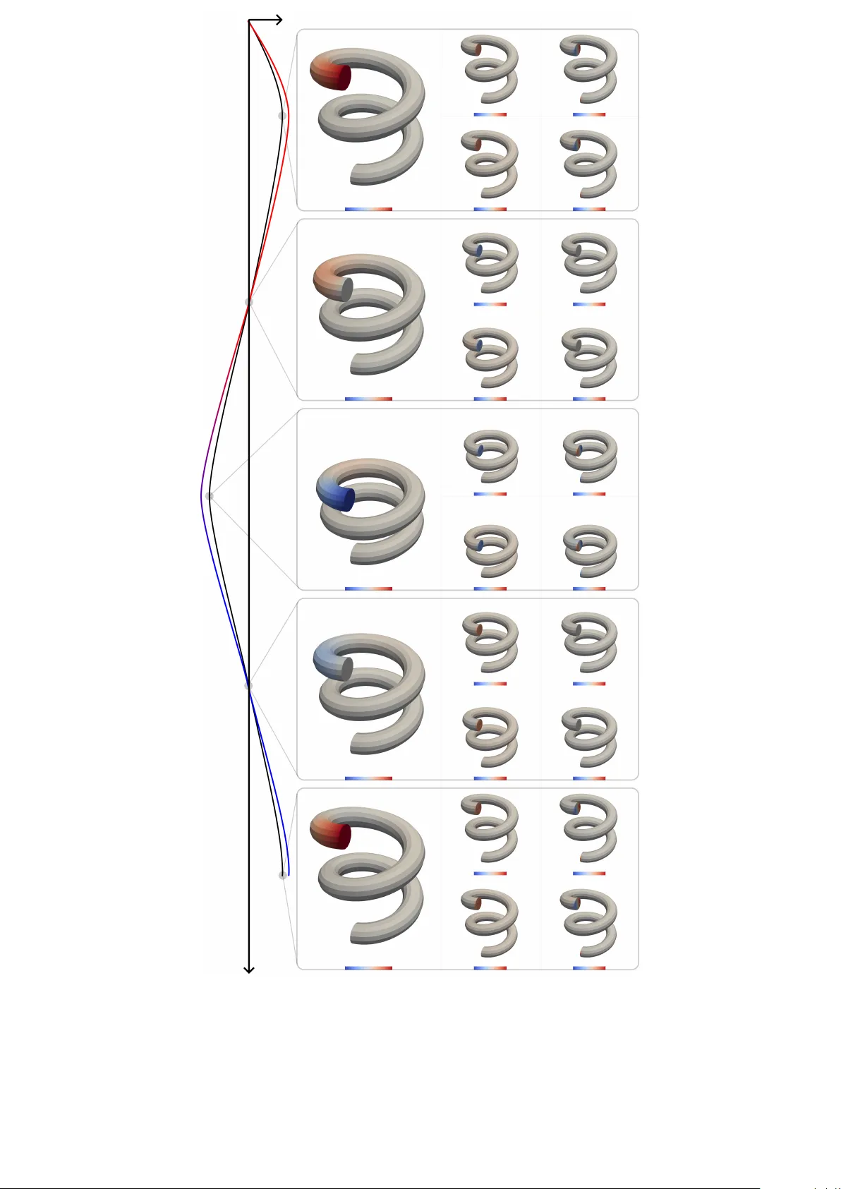
A Con v ex Route to Thermomec hanics: Learning In ternal Energy and Dissipation Hagen Holth usen a, ∗ , P aul Steinmann a , Ellen Kuhl a,b a Institute of Applie d Me chanics, University of Erlangen-Nur emb er g, Egerlandstraße 5, 91058 Erlangen, Germany b Dep artment of Mechanic al Engine ering, Stanfor d University, Unite d States Abstract W e presen t a physics-based neural net work framework for the discov ery of constitutive mo dels in fully coupled ther- momec hanics. In contrast to classical form ulations based on the Helmholtz energy , we adopt the in ternal energy and a dissipation p oten tial as primary constitutive functions, expressed in terms of deformation and entrop y . This choice a voids the need to enforce mixed con vexit y–concavit y conditions and facilitates a consistent incorp oration of thermo dynamic principles. In this contribution, we fo cus on materials without preferred directions or internal v ariables. While the formulation is posed in terms of entrop y , the temp erature is treated as the indep enden t observ able, and the en tropy is inferred internally through the constitutiv e relation, enabling thermodynamically consisten t modeling without requiring en tropy data. Thermo dynamic admissibilit y of the netw orks is guaran teed by construction. The internal energy and dissipation p o- ten tial are represen ted b y input con v ex neural net works, ensuring conv exity and compliance with the second law. Ob- jectivit y , material symmetry , and normalization are embedded directly in to the arc hitecture through inv ariant-based represen tations and zero-anchored formulations. W e demonstrate the performance of the proposed framework on syn thetic and experimental datasets, including purely thermal problems and fully coupled thermomechanical resp onses of soft tissues and ﬁlled rubb ers. The results show that the learned models accurately capture the underlying constitutiv e b ehavior. All co de, data, and trained models are made publicly a v ailable via Zeno do.org. Keywor ds: Thermo elasticit y, Neural netw orks, Internal energy, Dissipation p oten tial, Finite strains, Automated Mo del Discov ery, Finite Element Simulation 1. In tro duction Mec hanics and thermo dynamics are intrinsically intert wined. Whenever materials deform, they store energy , exc hange heat, and dissipate part of the supplied pow er through irrev ersible mec hanisms [1, 2, 3]. This in terpla y has been studied extensively in classical contin uum thermomechanics. Early thermo elastic form ulations already highlighted the coupling b et ween deformation and temp erature [4], while later dev elopments introduced internal-v ariable frameworks to describ e irrev ersible pro cesses [5, 6]. V ariational approaches further uniﬁed energy storage and dissipation within a consistent thermo dynamic setting [7, 8, 9]. Despite these adv ances, constructing constitutive mo dels that remain thermo dynamically consistent while capturing complex coupled resp onses across loading paths remains a challenging task. Recen t progress in physics-based machine learning aims to address this challenge by combining data-driven ﬂexibilit y with ph ysical structure. Within this con text, tw o complementary researc h directions hav e emerged, whic h diﬀer primarily in ho w physical principles are incorp orated into the learning pro cess. The ﬁrst direction fo cuses on constitutive mo deling based on str ongly-enfor cing netw ork arc hitectures. Here, neural net works are designed to represent material b eha vior directly , while thermo dynamic admissibility is ensured by con- struction through arc hitectural constraints. This idea has b een established in Constitutiv e Artiﬁcial Neural Netw orks ∗ Corresponding author Email addr esses: hagen.holthusen@fau.de (Hagen Holthusen), paul.steinmann@fau.de (Paul Steinmann), ekuhl@stanford.edu (Ellen Kuhl) Pr eprint submitted to Elsevier Mar ch 31, 2026 for automated mo del discov ery [10, 11] and Physics-Augmen ted Neural Netw ork form ulations [12]. An alternative net- w ork architecture relies on the concept of Kolmogoro v-Arnold Net works and is already applied for constitutive discov ery [13, 14, 15]. Subsequen t developmen ts impro ve robustness and ﬂexibility , for example through enhanced constrain t handling and parametrized mo del classes [16, 17, 18]. These approac hes ha ve b een successfully applied to increasingly complex inelastic materials [19, 20], for instance, visco elasticit y [21, 22, 23], plasticity [24, 25], strain-induced crystalliza- tion [26], growth and remo deling [27], and non-con vex anisotropic inelasticity [28]. A hierarc hy of thermo dynamically consisten t learning framew orks is recen tly presented in [29]. In the context of multiph ysical extensions, [30, 31] intro- duce magneto-elastic multiscale formulations. Overall, this line of work provides a p ow erful framework for learning constitutiv e relations that are consistent by construction. Complemen tary to this, the second direction is ro oted in partial diﬀerential equations and relies on we akly-enfor cing net work arc hitectures, most prominently Ph ysics-Informed Neural Netw orks (PINNs ) [32]. In this setting, the gov erning equations are embedded into the loss function, enabling the solution of forward and in verse b oundary v alue problems without explicit discretization sc hemes. Over the past y ears, PINNs ha ve ev olved into a versatile to ol for scientiﬁc machine learning [33, 34], with numerous applications in thermal mo deling. These include heat conduction in heterogeneous and anisotropic media [35, 36, 37], as w ell as coupled transp ort phenomena such as p orous and conjugate heat transfer [38, 39]. Suc h developmen ts demonstrate the capability of PINN-based approaches to handle strongly coupled ﬁeld problems. A t the interface of these tw o directions, ﬁrst studies addressing coupled thermomec hanical behavior hav e emerged. PINN-based approac hes hav e b een applied to thermo elasticit y , wa ve propagation, and p oroelasticity [40, 41, 42, 43], while classical contin uum formulations con tinue to provide the theoretical foundation for non-isothermal inelasticity at ﬁnite strains [44, 45, 46, 47]. More recen tly , gradient-enhanced and phase-ﬁeld models hav e b een developed to describ e coupled damage and failure pro cesses [48, 49, 50, 51]. How ever, a uniﬁed data-driven framework that combines constitutiv e learning with fully coupled thermomechanical consistency is still lacking. F rom a data-driv en constitutive p erspective, existing approaches typically rely on sp eciﬁc thermo dynamic p oten tials. Early work often prescrib es parts of the temp erature dep endence and fo cuses on learning the remaining constitutive resp onse [52]. More recent dev elopments incorp orate thermo dynamic structure directly into the netw ork architecture, most notably through form ulations based on the Helmholtz energy [53]. T o the authors’ kno wledge, the latter represents the ﬁrst strongly-enforcing net work architecture for thermomechanics. While these approaches ensure consistency for thermo elastic pro cesses, they do not address fully coupled thermomec hanical b eha vior with dissipation in a general setting. Researc h gap. Recen t progress in ph ysics-based neural netw orks for thermomechanics has primarily fo cused on thermo elastic constitutive mo deling. These approaches typically rely on Helmholtz energy form ulations with conv exity- lik e constrain ts in deformation and concavit y in temp erature. While this provides a rigorous framew ork for thermo- h yp erelasticit y , the extension to fully coupled thermomechanical pro cesses with dissipation remains largely unexplored. In particular, a general framework that incorp orates irrev ersible thermal eﬀects, embeds thermomechanical principles by construction, and remains compatible with the observ able temp erature ﬁeld is still an op en challenge. Aim of the study . The aim of this work is to develop a physics-based neural netw ork framework for the discov ery of constitutiv e models in fully coupled thermomechanics. T o this end, we formulate the constitutiv e b eha vior in terms of the in ternal energy and a dissipation p oten tial, while treating temperature as the independent observ able and entrop y as an auxiliary v ariable inferred through the constitutive relation. This choice av oids the mixed conv exity–conca vity requiremen ts of Helmholtz-based form ulations and enables a thermo dynamically consisten t treatment of dissipativ e thermomec hanical pro cesses. Building on this foundation, we construct neural netw ork architectures that satisfy ther- mo dynamic admissibility and fundamental material principles by design. Outline. The remainder of this contribution is organized as follows. In Section 2, the thermomec hanical framework is in tro duced, including the internal energy form ulation and the underlying thermodynamic structure. The neural net work architecture and the em b edding of thermo dynamic constraints are presented in Section 3. Subsequen tly , a series of n umerical examples is in vestigated: a purely thermal problem (Section 4.1), temp erature-dep enden t mechanical b eha vior of exp erimental datasets (Sections 4.2 and 4.3), and a fully coupled structural setting (Section 4.4). The results are analyzed and discussed in Section 5, follo wed by concluding remarks. 2 2. Theoretical foundations W e aim to design a neural netw ork architecture that satisﬁes the gov erning principles of thermomechanics a priori . F or this purp ose, we consider the contin uum mechanical form ulation of a fully coupled thermomechanical problem in the reference conﬁguration. W e ﬁrst state the dissipation requirement and introduce constitutiv e p otentials that ensure thermo dynamic admissibility . W e then summarize the balance equations for the coupled mechanical and thermal ﬁelds. Building on this foundation, we dis cuss material principles that are mandatory for admissible constitutive mo deling, with a fo cus on isotropic materials. Thereafter, we outline additional material constraints that are not strictly required by the balance laws and the second law, but are highly b eneﬁcial when constructing robust and reliable netw ork architectures. W e conclude with the discretized weak forms of the balance equations. Thermo dynamic p oten tials. In solid mec hanics, the Helmholtz energy is commonly employ ed b ecause it represents the mechanically a v ailable energy and admits the natural v ariables deformation gradient F and absolute temp erature T > 0 . Ho wev er, thermo dynamic stability requires conca vity of the Helmholtz energy with respect to T , together with mechanical stability conditions that are typically expressed through conv exity-t yp e requirements in appropriate deformation measures. Imp osing these mixed curv ature prop erties directly within neural net work parametrizations is non-trivial. W e therefore adopt the internal energy e and describe the material state in terms of the pair ( F , s ) , where s denotes the referential en trop y density . The constitutiv e structure is characterized by an energetic p otential and a dissipation p oten tial, e = e ( F , s ) , ϕ = ϕ ( ˙ F , ˙ s, g ; F , s ) , (1) where the semicolon indicates that ( F , s ) act solely as parameters of the dissipation p otential. The dissipation p oten tial ϕ accounts for irreversible pro cesses in the sense of generalized standard materials [6, 3]. The referential thermal gradient is deﬁned as g := − 1 T Grad( T ) = − Grad(ln( T )) , (2) whose con tribution to ϕ is consistent with the concept of a conduction p oten tial prop osed in [4]. It is imp ortan t to emphasize that, although the core formulation is expressed in terms of ( F , s ) , entrop y is not measured directly in exp erimen ts. Instead, the temperature ﬁeld T is accessible. Through the constitutiv e relation linking T and s , we infer the corresponding en tropy from the prescrib ed deformation and temperature ﬁelds. Hence, while the model is form ulated in terms of the internal energy and entrop y , it remains fully compatible with measurable quantities 1 . Clausius–Duhem inequality . T o construct a constitutive framework that is thermo dynamically admissible by design, w e start from the second law of thermo dynamics in its lo cal form. In the reference conﬁguration, the Clausius–Duhem inequalit y reads P : ˙ F − ˙ e + T ˙ s + q · g ≥ 0 , (3) where P denotes the Piola stress tensor and q the referential heat ﬂux. Using the constitutive p oten tials in Eq. (1), we p ostulate the state laws P − ∂ e ∂ F = ∂ ϕ ∂ ˙ F , T − ∂ e ∂ s = ∂ ϕ ∂ ˙ s , q = ∂ ϕ ∂ g , (4) whic h deﬁne stress, temp erature, and heat ﬂux directly in terms of the energetic and dissipative p oten tials. In particular, the second relation establishes the link b et ween the measurable temp erature ﬁeld and the entrop y , whic h will pla y a cen tral role in our discov ery framework. Balance equations. While the Clausius–Duhem inequality constrains the lo cal constitutive resp onse, th e ev olution of the mechanical and thermal ﬁelds is go verned by the corresponding balance laws. In the reference conﬁguration and neglecting inertia for clarit y , the balance of linear momentum is given by Div P + f = 0 , (5) 1 The relations induced by Legendre transformations b et ween the internal energy and the Helmholtz energy , as well as the transformation of the dissipation p oten tial with respect to the entrop y rate ˙ s and its conjugate v ariable, are closely connected to v ariational formulations of thermomechanics. The interested reader is referred to [7] for a detailed discussion. 3 where f denotes the referential b o dy force. The balance of internal energy reads ˙ e = P : ˙ F − Div q + r, (6) with referential heat source r . T ogether with suitable Diric hlet and Neumann b oundary conditions for the deformation and temp erature ﬁelds, these equations deﬁne the fully coupled thermomechanical b oundary v alue problem. 2.1. Material principles W e now discuss fundamen tal material principles that constitute mandatory requirements for admissible constitutiv e mo deling. In the follo wing, we restrict our attention to isotropic materials, that is, materials without preferred in ternal directions. Ob jectivity . The principle of ob jectivit y requires inv ariance of the constitutive resp onse under sup erposed rigid b o dy motions. F or ev ery time-dep enden t rotation tensor Q ( t ) ∈ SO(3) , the internal energy and the dissipation p oten tial must satisfy e ( F , s ) = e ( QF , s ) , ϕ ( ˙ F , ˙ s, g ; F , s ) = ϕ ( ˙ QF , ˙ s, g ; QF , s ) , (7) where ˙ QF denotes the material time deriv ativ e of QF . Note that g is a referential quan tity . In addition, all constitutively determined quantities m ust transform consistently . In particular, the Piola stress tensor and the referential heat ﬂux are required to satisfy QP ( F , s, ˙ F , ˙ s, g ) = P ( QF , s, ˙ QF , ˙ s, g ) , q ( F , s, ˙ F , ˙ s, g ) = q ( QF , s, ˙ QF , ˙ s, g ) . (8) Since the absolute temp erature T is a scalar ﬁeld, it is inv ariant under sup erposed rigid b o dy motions. Material symmetry . The principle of material symmetry states that the material resp onse must b e inv ariant under sup erposed time-indep enden t rotations of the reference conﬁguration that b elong to the symmetry group of the material. F or isotropic materials, this symmetry group coincides with the full special orthogonal group, that is Q ∈ SO(3) . A ccordingly , the constitutive p oten tials are required to satisfy e ( F , s ) = e ( F Q , s ) , ϕ ( ˙ F , ˙ s, g ; F , s ) = ϕ ( ˙ F Q , ˙ s, Q T g ; F Q , s ) , (9) and the asso ciated constitutive quantities must fulﬁll P ( F , s, ˙ F , ˙ s, g ) Q = P ( F Q , s, ˙ F Q , ˙ s, Q T g ) , Q T q ( F , s, ˙ F , ˙ s, g ) = q ( F Q , s, ˙ F Q , ˙ s, Q T g ) . (10) The absolute temp erature again satisﬁes this requirement trivially , since it is a scalar quantit y . Com bining ob jectivit y and material symmetry for isotropic materials, the in ternal energy and the dissipation potential can b e regarded as sc alar-value d isotr opic functions , e ( F , s ) = e ( C , s ) , ϕ ( ˙ F , ˙ s, g ; F , s ) = ϕ ( ˙ C , ˙ s, g ; C , s ) , (11) dep ending on the right Cauch y–Green tensor C = F T F and its rate. With this represen tation and the state laws (4), the transformation prop erties in Eqs. (8) and (10) are satisﬁed. 2.2. Material c onstr aints The following constrain ts are not strictly required by the balance la ws and the Clausius–Duhem inequality . How ever, they are frequently imp osed in order to improv e stability , identiﬁabilit y , and extrap olation prop erties of learned constitutive mo dels. In this sense, they serv e as guiding principles for the design of our physics-based neural netw ork architecture. 4 Standard dissipative solids. So far, the dissipation p oten tial allows us to accoun t for dissipativ e eﬀects related to b oth deformation and thermal pro cesses. The former is typically asso ciated with ﬂuid-like or viscous material b eha vior, whereas the latter b ecomes relev ant for pronounced temp erature gradients or rapid thermal pro cesses, for instance under strong transien t heating. In the present work, we restrict ourselv es to the class of standard dissipative solids. A ccordingly , we neglect the pair ( ˙ F , ˙ s ) in the argument list of ϕ , while still allowing the p oten tial to b e parameterized by ( F , s ) . Under this assumption, the state la ws (4) reduce to P = ∂ e ∂ F , T = ∂ e ∂ s > 0 , (12) whic h implies that the internal energy is monotonic al ly incr e asing with resp ect to the en tropy . Normalization. When the material is in its rest state, it is common to imp ose normalization conditions on the p oten tials as well as on the constitutiv ely dep enden t quantities. The rest state is characterized by a deformation gradient equal to the identit y tensor, a reference temp erature T 0 > 0 , and the corresp onding reference entrop y s 0 . While the reference temp erature must b e strictly p ositiv e, the reference entrop y is less constrained. A common choice in contin uum mec hanics is to set s 0 = 0 at T = T 0 , whic h we adopt here 2 . The normalization conditions for the p oten tials therefore read e ( I , 0) = 0 , ϕ ( 0 ; F , s ) = 0 . (13) The latter condition expresses that the dissipation p otential v anishes in the absence of its driving force, indep endently of the parametrization. F or the stress and temp erature, we analogously obtain P ( I , 0) = ∂ e ∂ F     F = I s =0 = 0 , T ( I , 0) = ∂ e ∂ s     F = I s =0 = T 0 . (14) Con v exity of the in ternal energy . The reduced temp erature relation in Eq. (12) provides a constitutive link b et ween en tropy and temp erature. Up to this p oin t, how ever, this relation is not necessarily uniquely inv ertible. While each en tropy v alue yields a unique temp erature, a given temp erature could, in principle, correspond to multiple entrop y v alues. Such b eha vior may arise, for example, in the presence of phase transformations, which are not considered in the presen t work. W e therefore additionally require ∂ 2 e ∂ s 2 > 0 , (15) that is, strict c onvexity of the internal energy with resp ect to the entrop y . Similarly , we imp ose conv exit y-related conditions with resp ect to F . Since conv exity in F is generally to o restrictive in ﬁnite elasticity , we adopt the concept of polyconv exity [54]. T ogether with coercivity , p olycon vexit y pro vides a suﬃcien t condition for the existence of minimizers [55]. In the thermomec hanical setting, the internal energy is said to b e p olycon vex if it admits a representation e = W ( F , cof F , J ; s ) , (16) whic h is con vex in ( F , cof F , J ) for ﬁxed entrop y s . Here, cof F denotes the cofactor of the deformation gradien t and J its determinan t. A subtle but imp ortan t p oint is that the energy is required to b e jointly c onvex in ( F , cof F , J ) and conv ex in s , whereas b et ween s and the set ( F , cof F , J ) only sep ar ate c onvexity is imp osed. Consequently , for the extended set of v ariables ( F , cof F , J, s ) the full Hessian is not required to b e p ositiv e (semi-)deﬁnite. Con v exity of the dissipation p oten tial. Since we restrict ourselves to standard dissipativ e solids, the deriv atives of ϕ with resp ect to ˙ F and ˙ s v anish identically . F or the remaining contribution q · g in the dissipation inequalit y (3), appropriate structural restrictions on the dissipation p oten tial are required. T o this end, we recall a classical result from con vex analysis [56]. If the p otential satisﬁes ϕ ( 0 ; F , s ) = 0 , ϕ ( g ; F , s ) ≥ 0 , ϕ ( 0 ; F , s ) ≥ ϕ ( g ; F , s ) − ∂ g ϕ · g , (17) 2 F or instance, a standard choice for the caloric part of the Helmholtz energy ψ ( T ) = c T 0 [ T − T 0 − T ln( T T 0 )] , diﬀerentiation with resp ect to T yields an entrop y satisfying s 0 = 0 at T = T 0 . Here, c T 0 denotes the heat capacity . 5 then the Clausius–Duhem inequalit y is satisﬁed [57]. Here, ∂ g ϕ denotes the subgradien t of ϕ with resp ect to g . While Eq. (17) essen tially enforces con vexit y of the potential, con vexit y is only a suﬃcien t, not a necessary , condition. More general formulations based on monotone p oten tials and their incorp oration in to physics-based neural netw orks can b e found in [28]. In the present work, how ever, we restrict ourselves to conv ex dissipation p oten tials. 2.3. W e ak forms and their line arization The in ternal energy and the dissipation p oten tial are represented by physics-based neural netw orks. F or the identiﬁcation of the constitutive b eha vior, we adopt an unsup ervised learning strategy . Accordingly , the neural netw ork representations of the internal energy and the dissipation p oten tial are embedded into a temp oral and spatial discretization of the balance la ws Eqs. (5) and (6). This results in a weak formulation of the coupled thermomechanical b oundary v alue problem, whic h forms the basis of the numerical implementation. Principle of virtual work. F or a given displacement ﬁeld u and the temp erature ﬁeld T , the internal and external virtual w ork must b e in equilibrium, w tot := w int − w ext ! = 0 . (18) The in ternal virtual work is given by w int := Z B P : Grad( δ u ) d V + Z B [ T ˙ s δ T − q · Grad( δ T )] d V , (19) where δ u and δ T denote admissible test functions for the mec hanical and thermal ﬁelds, resp ectiv ely . The ﬁrst term corresp onds to the virtual work of the stresses, while the remaining terms represent the weak form of the thermal balance, expressed in terms of the en tropy rate and the heat ﬂux. The external virtual w ork reads w ext := Z B f · δ u d V + Z ∂ B t t · δ u d A + Z B r δ T d V + Z ∂ B q q δ T d A, (20) where t denotes the prescrib ed traction on the Neumann b oundary ∂ B t and q refers to the prescrib ed heat ﬂux on ∂ B q . On the Diric hlet b oundaries, the essential b oundary conditions u = ˜ u , T = ˜ T (21) are imp osed. On the Neumann b oundaries, the natural b oundary conditions are given by P · n = t , q · n = − q , (22) where n denotes the out ward unit normal vector in the reference conﬁguration. Spatial and temporal discretization. In space, we adopt an isoparametric ﬁnite elemen t discretization. The displacemen t and temp erature ﬁelds are approximated as u h ( X ) = n node X a =1 N a ( X ) u a , T h ( X ) = n node X a =1 N a ( X ) T a , (23) where N a denote the shap e functions and u a , T a the corresponding no dal degrees of freedom. The same interpolation functions are emplo yed for the geometrical mapping. F or the temp oral discretization, we use an implicit backw ard Euler sc heme for the entrop y rate, ˙ s n +1 = s n +1 − s n ∆ t , (24) with time increment ∆ t . All constitutiv e quantities are ev aluated at time level n + 1 , leading to a fully coupled nonlinear system at eac h time step. The entrop y is treated as an auxiliary v ariable and is determined implicitly from the state la w (12) T n + α − ∂ e n + α ∂ s n + α = 0 , α ∈ { 0 , 1 } , (25) whic h is solved lo cally at each quadrature p oin t and time level. Insertion of the discretized ﬁelds in to the weak form yields a nonlinear algebraic system in residual form, r =  r u ( u h , T h ) ∆ t r T ( u h , T h )  = 0 , (26) 6 where the global residual v ector collects the mec hanical and thermal contributions. The thermal residual is scaled b y the time increment ∆ t to improv e numerical conditioning. In analogy to the pro cedure of pseudo p otentials [58], the individual residual v ectors are obtained by diﬀerentiating the discretized total virtual work with resp ect to the corresp onding global vectors ( • ) glo of no dal trial v alues, r u = ∂ w h tot ∂ δ u h glo , r T = ∂ w h tot ∂ δ T h glo . (27) Since the trial v alues enter the weak form linearly , these deriv atives are indep enden t of their sp eciﬁc representation and can b e ev aluated eﬃcien tly using algorithmic diﬀerentiation. The global residual in Eq. (26) plays a central role in the disco very pro cedure, as it serves as the physics-based loss term enforcing the balance laws at the discrete level. 3. Ph ysics-based neural net w ork architecture With the theoretical foundations of the previous section, w e are no w enabled to design a physics-based neural net work arc hitecture that satisﬁes ph ysics a priori . T o this end, w e will learn both the in ternal energy e and the dissipation p oten tial ϕ by means of ph ysics-constraint neural netw orks. As w e ha ve seen, conv exity for b oth p oten tials is an essen tial ingredient. T o this end, we will employ Input Conv ex Neural Netw orks (ICNNs) [59] to construct generally con vex net works. W e will address how to incorp orate the material principles discussed in Section 2.1 and constraints in Section 2.2 in to the ov erall architecture 3.1. Zer o-Anchor e d Neur al Networks In the following, w e introduce the general arc hitecture of the neural netw orks employ ed in this con tribution. In Sec- tion 3.2, we discuss ho w these arc hitectures are tailored to the requiremen ts of join t and separate conv exity for the internal energy , the conv ex dissipation p oten tial b eing parameterized by ( F , s ) , and the prediction of entrop y for stabilizing the training pro cess. F ully Input Conv ex Neural Net w ork. T o b egin with, we comment on fully Input Conv ex Neural Netw orks (FIC- NNs). Their construction relies on three fundamental prop erties of conv ex functions: the sum of conv ex functions is con vex, a non-negativ e scaling of a conv ex function remains con vex, and the comp osition f ◦ g is conv ex if f is con vex and monotonically non-decreasing and g is con vex. Based on these principles, the arc hitecture reads x 1 = σ 0 ( V 0 x 0 + b 0 ) − σ 0 ( b 0 ) , x ℓ +1 = σ ℓ ( W ℓ x ℓ + V ℓ x 0 + b ℓ ) − σ ℓ ( b ℓ ) , (28) where the activ ation functions σ ℓ are required to b e conv ex and monotonically non-decreasing. The weigh t matrices in the recurren t branch satisfy W ℓ ∈ R ≥ 0 , while initially V ℓ ∈ R . Additionally , there are no constraints imp osed on the biases. The subtraction of σ ℓ ( b ℓ ) is in line with [28] and ensures that the netw ork is zero-anchored, i.e., the output v anishes for v anishing input without aﬀecting conv exit y . In our setting, conv ex functions are often pro vided as inputs to the ICNN rather than the raw argumen ts. T o preserve con vexit y under such comp ositions, w e additionally restrict V ℓ ∈ R ≥ 0 . P artially Input Con vex Neural Netw orks. While the internal energy dep ends exclusiv ely on arguments for which con vexit y is required, the dissipation p oten tial may b e parameterized by F and s . F or this reason, we employ a partially Input Con vex Neural Netw ork (PICNN) [59], slightly adapted following [28], x c 1 = σ 0  V c 0  x c 0 ⊙ [ V cp 0 x p 0 + b cp 0 ] +  + U cp 0 x p 0 + b c 0  − σ 0 ( U cp 0 x p 0 + b c 0 ) , x c ℓ +1 = σ ℓ  W c ℓ h x c ℓ ⊙ [ W cp ℓ x p ℓ + b cp ℓ ] + i + V c ℓ h x c 0 ⊙ [ V cp ℓ x p ℓ + c cp ℓ ] + i + U cp ℓ x p ℓ + b c ℓ  − σ ℓ ( U cp ℓ x p ℓ + b c ℓ ) , x p ℓ +1 = f ℓ ( W p ℓ x p ℓ + b p ℓ ) − f ℓ ( b p ℓ ) , (29) where [ • ] + denotes the ReLU activ ation. All weigh ts associated with the con vex branch ( • ) c are constrained to b e non-negativ e in order to preserve conv exity . In contrast, neither the weigh ts nor the activ ation functions f ℓ in the parameterization branc h ( • ) p , nor the w eights app earing in the coupling terms ( • ) cp , are sub ject to sign constraints. Finally , we emphasize a crucial diﬀerence compared to neural net works employing ICNNs for elastic [18, 12] and inelastic materials [28, 22]. In the present setting, strict conv exit y with resp ect to the entrop y is required. Although monotonicity 7 is preserved under composition with increasing conv ex functions, multiplication by zero would reduce a strictly con vex function to a merely con vex one. T o prev ent suc h degeneracy , all weigh ts asso ciated with the con vex branc h are constrained to b e strictly p ositiv e. Auxiliary Multila yer P erceptron. Although the en trop y can b e obtained by iteratively solving Eq. (25), this approac h may b e ineﬃcient during training. The reason is that automatic diﬀerentiation would need to propagate gradien ts through all iterations of the solver unless implicit diﬀerentiation is employ ed. As an alternative, we approximate the en tropy using an auxiliary multila yer p erceptron (MLP) x ℓ +1 = f ℓ ( W ℓ x ℓ + b ℓ ) − f ℓ ( b ℓ ) , (30) whic h is anc hored at the origin in the same manner as the previously introduced net works. No additional constraints are imp osed on the activ ation functions, weigh ts, or biases. After training, the iterative solver of Eq. (25) is reintroduced during inference. Loss function. The training ob jectiv e consists of a physics-based loss, a regularization term, and an auxiliary loss, L = λ D L D + λ N L N | {z } L phys + λ R L R + λ A L aux . (31) The physics loss L phys enforces the discrete balance laws and is constructed from the global residual vector introduced in Eq. (26). It is decomp osed into contributions asso ciated with Dirichlet b oundaries and Neumann b oundaries (including free no des), where λ D and λ N are scaling parameters. Eac h contribution is deﬁned as the mean squared error of the corresp onding residual comp onen ts. Denoting by r D and r N the residual v ectors asso ciated with Dirichlet and Neumann b oundaries, resp ectiv ely , we deﬁne L D = MSE( r D ) , L N = MSE( r N ) . (32) T o ensure a consisten t scaling of the residual contributions, the external loads entering the weak form are normalized. In particular, the prescrib ed mechanical tractions and bo dy forces, as w ell as the thermal ﬂuxes and heat sources, are scaled suc h that their resp ectiv e maxim um absolute v alues are equal to one. This normalization, indicated by ( • ) , is p erformed separately for the mechanical and thermal problems based on their individual maximal absolute load v alues. Consequen tly , the mechanical and thermal contributions are scaled indep enden tly , prev enting an artiﬁcial imbalance b et ween the tw o ﬁelds. The regularization term L R is introduced to enhance the stability of the training pro cedure and to control the complexity of the neural netw orks. In particular, sparsit y-promoting regularization can b e employ ed to drive insigniﬁcan t parameters to wards zero, which is b eneﬁcial from b oth a mec hanical interpretation and a mo del reduction p erspective. T o this end, the regularization term is formulated as a p enalty on the parameter tensors of selected subnetw orks. Considering the parameter tensors W i , V i , U i , and b i asso ciated with subnetw ork i , a combination of L 1 - and L 2 -t yp e contributions is emplo yed to balance sparsity and smo othness, i.e., L R = X i ∈J reg X P ∈{ W i , V i , U i , b i } h λ (1) i ∥ P ∥ 1 + λ (2) i ∥ P ∥ 2 F i , (33) where ∥ P ∥ 1 = P k | P k | denotes the entry-wise L 1 -norm and ∥ P ∥ F the F rob enius norm. Here, J reg denotes the set of subnet works sub ject to regularization, and λ (1) j , λ (2) j are the corresp onding regularization co eﬃcien ts. Finally , the auxiliary loss enforces consistency b et ween the thermo dynamic state law Eq. (12) and the entrop y predicted b y the auxiliary MLP introduced in Eq. (30). It is deﬁned as L aux = MSE  T n +1 − ∂ e n +1 ∂ s n +1  , (34) and is ev aluated at each quadrature p oin t in the domain. 3.2. Neur al network r epr esentation of internal ener gy, dissip ation p otential, and entr opy After we in tro duced the general neural net work architectures, we no w detail their sp eciﬁc design for the internal energy and the dissipation p otential, which satisﬁes the material principles and constrain ts outlined in Sections 2.1 and 2.2. F urthermore, we describ e the design for the prediction of entrop y . An ov erview of the netw ork architecture and the in teractions b et ween the subnetw orks is provided in Fig. 1. 8 F T g s ∗ + P q FICNN F ,s FICNN F FICNN s PICNN g MLP s ∂ ∂ F ∂ ∂ g Figure 1: Overall network architecture consisting of the subnetw orks MLP s , FICNN s , FICNN F , FICNN F ,s , and PICNN g , together with their interactions. In a ﬁrst step, the entrop y s is predicted by MLP s . Subsequen tly , s and the deformation gradient F are provided as inputs to the resp ectiv e subnetw orks, from which the ﬁrst Piola–Kirchhoﬀ stress P is obtained via diﬀerentiation. In parallel, the referential heat gradient g is pro cessed by PICNN g , which is additionally parameterized by ( F , s ) , yielding the referential heat ﬂux q through diﬀerentiation. In ternal energy . W e b egin by sp ecifying the material principles imp osed on the internal energy . As discussed ab o v e, the internal energy is formulated as a scalar-v alued isotropic function and is therefore expressed in terms of the principal in v ariants [60, 61, 62] I 1 := tr( C ) , I 2 := tr(cof C ) , J := det( F ) , (35) whic h ensure ob jectivit y and material symmetry and pro vide a p olycon vex set of arguments. All inputs are shifted with resp ect to the rest conﬁguration F = I , ¯ I 1 := I 1 − 3 , ¯ I 2 := I 2 − 3 , ¯ J := J − 1 , ¯ s := s − s 0 , (36) suc h that the reference state corresponds to zero input. Based on these ingredien ts, w e p ostulate the following decom- p osition of the internal energy , e ( F , s ) = n T  ˆ e ( F , s ) + e gr ( F ) − n P ¯ J  , (37) where the individual con tributions are introduced in the following. T o construct a conv ex represen tation, w e introduce an auxiliary internal energy ˆ e based on fully input-conv ex neural net works (FICNNs), cf. Eq. (28), ˆ e ( F , s ) = FICNN F ,s  [ ¯ I 1 , ¯ I 2 , ¯ J , − ¯ J , ¯ s ]  +  FICNN F  [ ¯ I 1 , ¯ I 2 , ¯ J , − ¯ J ]  + ∗ { FICNN s ( ¯ s ) } + − n { 0 } 2 + , (38) where FICNN F ,s is scalar-v alued, whereas FICNN F and FICNN s pro duce feature vectors of equal dimension. The Softplus activ ation function is denoted by {•} + , and the op erator ∗ denotes the element wise product follo wed by summation o ver the feature dimension, such that the resulting contribution is scalar-v alued. The parameter n corresp onds to the n umber of output features, and the subtraction term ensures prop er normalization in the trivial case FICNN F = FICNN s = 0 . The ab o ve decomp osition reﬂects the partially separable conv ex structure of the internal energy: the ﬁrst term captures join t conv exity in deformation and entrop y , while the second term enriches the representation through additional separable con vex contributions. Since p olyconv exity alone is not suﬃcient to guarantee the existence of minimizers, a suitable co erciv e growth b eha vior of the energy is additionally required. T o promote this prop ert y , we augment the internal energy by a small growth con tribution, e gr ( F ) = ϵ gr [[ I 1 − 3 − ln(det( C ))] + [ I 2 − 3 − ln(det(cof C ))] + [ J − 1 − ln( J )]] = ϵ gr  ¯ I 1 + ¯ I 2 + ¯ J − 7 ln( J )  , (39) where ϵ gr > 0 is chosen suﬃcien tly small. This term enhances the gro wth of the energy under large distortional deformations and preven ts volumetric collapse as J → 0 . Notably , e gr satisﬁes the normalization conditions of b oth energy and stress. 9 W e next enforce the normalization condition of the Piola stress tensor stated in Eq. (14). F ollowing [18], w e in tro duce the stress normalization factor n P =  2 ∂ ˆ e ∂ I 1 + 4 ∂ ˆ e ∂ I 2 + ∂ ˆ e ∂ J      F = I s =0 , (40) whic h corresp onds to the stress scaling at the reference conﬁguration. In addition, temp erature normalization is imp osed via n T = T 0 " ∂ ˆ e ∂ s     F = I s =0 # − 1 . (41) Since the auxiliary energy is constructed to b e monotonically increasing with resp ect to entrop y , the deriv ative ∂ ˆ e/∂ s is strictly p ositiv e, ensuring that this normalization is well-deﬁned. Moreov er, due to the adopted ICNN architecture, the normalization condition of the energy is satisﬁed b y construction. Dissipation p oten tial. Lastly , we represent the dissipation p oten tial by a neural netw ork. Analogous to the in ternal energy , it is formulated as a scalar-v alued isotropic function. F ollowing [62], we introduce the inv ariants I 4 := g · g , I 5 := g · C · g , I 6 := g · cof C · g . (42) F urther, we reform ulate these quan tities in te rms of tensor-induced norms. F or a symmetric p ositiv e deﬁnite tensor A , w e deﬁne ∥ v ∥ A := √ v · A · v , (43) whic h satisﬁes absolute homogeneit y and the triangle inequalit y and is therefore conv ex in v . Using this construction, w e introduce the mo diﬁed inv arian ts ¯ I 4 := ∥ g ∥ I , ¯ I 5 := ∥ g ∥ C , ¯ I 6 := ∥ g ∥ cof C , (44) whic h preserve isotropy and ensure con vexit y with resp ect to g . The dissipation p otential is then represented by a partially Input Con vex Neural Netw ork (PICNN), see Eq. (29), ϕ ( g ; F , s ) = PICNN g  [ ¯ I 4 , ¯ I 5 , ¯ I 6 ] , [ ¯ J , ¯ s ]  , (45) whic h is conv ex with resp ect to g while b eing parameterized by ¯ J and ¯ s . Additional scaling by inv arian ts such as ¯ I 1 or ¯ I 2 is omitted, since the dep endence on F and its cofactor is already captured through ¯ I 5 and ¯ I 6 . Due to the adopted architecture, the dissipation p oten tial satisﬁes ϕ ( 0 ; F , s ) = 0 by construction. Non-negativity is ensured b y applying an appropriate non-negative activ ation function to the scalar output neuron. Noteworth y , a shifted activ ation function must b e omitted for the output la yer; otherwise, also non-negative output functions such as ReLU ma y pro duce negative v alues. Consequently , the arc hitecture guarantees non-negative dissipation by design, cf. Eq. (17). Auxiliary entrop y net work. Lastly , we sp ecify the auxiliary m ultilay er p erceptron (MLP) in Eq. (30), which is emplo yed during training to predict the entrop y s . T o this end, w e introduce the temperature shift with resp ect to the reference state ¯ T := T − T 0 , (46) whic h, together with the shifted deformation inv ariants, serves as input to the netw ork. Accordingly , the en tropy is appro ximated as s = MLP s  [ ¯ I 1 , ¯ I 2 , ¯ J , ¯ T ]  . (47) Since the entrop y in the reference conﬁguration is chosen as s 0 = 0 , the zero-anchored arc hitecture of the MLP is consisten t with this normalization. After training, the auxiliary MLP is replaced by the iterative solv er enforcing the implicit state la w for the entrop y in Eq. (12). 4. T raining and T esting In the follo wing, we examine the prop osed physics-based netw ork arc hitecture for learning constitutive b eha vior in ther- momec hanics. T o this end, we study four diﬀerent test cases: tw o based on exp erimental data, presented in Sections 4.2 and 4.3, and tw o based on synthetic data, presen ted in Sections 4.1 and 4.4. The ﬁrst three examples address behavior at the material-p oin t level, or ov er a small spatial domain in the case of transien t heat diﬀusion. In the ﬁnal example, 10 w e inv estigate the abilit y of the architecture to learn from full-ﬁeld data and assess its accuracy in predicting no dal reactions for an unseen b oundary v alue problem. In this study , w e do not address the measuremen t of ph ysical ﬁelds, suc h as displacemen t, temp erature, and their asso ciated reactions, and instead assume full access to all ﬁelds. Although this is clearly an idealized setting, the training of physics-based neural netw orks and the asso ciated acquisition of exp erimen tal data constitute a substantial researc h topic in their own right. The inﬂuence of the displacement ﬁeld on the constitutive b eha vior arises primarily through its spatial gradient and time rate. This contrasts with the temp erature ﬁeld, which enters the form ulation indirectly through b oth the internal energy and the dissipation potential via the entrop y . In our experience, and consistent with common practice in the machine learning comm unity , this tends to bias the training tow ard the en tropy/temperature contribution, whose magnitude is generally larger than that of the spatial and temp oral gradien ts. Therefore, in line with the normalization pro cedure of the loss introduced in Eq. (32), we track the maximum temp erature during training and normalize the entire temp erature ﬁeld by this v alue. As a consequence, the temp erature gradients are scaled accordingly . During testing, this normalization v alue must b e taken into account when ev aluating unseen problems. In all examples, we employ the relative activity of the individual subnetw orks as an ev aluation metric. T o this end, w e quantify the activity of each subnet work by aggregating the norms of its parameters (weigh ts and biases). More sp eciﬁcally , for eac h parameter tensor W i , V i , U i , and b i , an activity measure is computed as its F rob enius norm, and subsequen tly summed o ver all parameters belonging to the resp ectiv e subnetw ork i . Denoting the resulting activit y of subnet work i by A i , the relativ e activity is deﬁned as ˜ A i = A i P j A j , (48) whic h represents the normalized contribution of each subnetw ork to the ov erall mo del activity . The ph ysics-based netw ork is implemented in JAX using the Flax pack age. Unless stated otherwise, all hyperparameters (training, constraints, regularization) and netw ork architectures are k ept iden tical across the examples. Their sp eciﬁc v alues are summarized in App endix A. F urthermore, the synthetic data are generated using the constitutive mo dels presented in App endix B. Notably , these mo dels are formulated in terms of the Helmholtz energy and a temperature-based dissipation p oten tial. Hence, w e do not explicitly prescrib e within the net work architecture the constitutiv e mo del used to generate the data; rather, during training, the netw ork must learn the intrinsic relation implied by the Legendre transformation. F or completeness, a brief summary of the constitutive equations in terms of the Helmholtz energy is provided in App endix C. 4.1. Synthetic data: He at diﬀusion T o b egin with, we consider the discov ery of the constitutive b eha vior of a purely transien t heat problem, i.e., a rigid heat conductor. Due to its transient nature, b oth the internal energy associated with the heat capacity and the dissipation p oten tial gov erning the heat ﬂux are non-zero. As sho wn in App endix B, we assume F ourier’s law for the heat ﬂux. F rom the p ersp ectiv e of the dissipation p oten tial (here equiv alent to a conduction p oten tial), F ourier’s la w induces a sp eciﬁc parametrization with resp ect to the temp erature or, equiv alently , the entrop y . Consequently , the netw ork is required to learn this parametrization from the data. The boundary v alue problem is lo osely inspired by experimental setups for the measurement of U -v alues in civil engi- neering applications [63]. While heat ﬂuxes and temp eratures are rep orted in the literature, t ypically only the ﬂuxes at the interior and exterior b oundaries are measured. How ever, for the identiﬁcation of transien t b eha vior, access to the temp erature ﬁeld across the w all is required. Otherwise, one is restricted to assuming a constant temp erature gradient, whic h is not consistent with transient heat conduction. Fig. 2 illustrates the considered b oundary v alue problem. In accordance with realistic building conditions, the exterior temp erature follows a sin usoidal v ariation ov er time, whereas the interior temperature is assumed to remain constant, cf. [63]. The domain is discretiz ed using 64 hexahedral eleme n ts with an edge length of 0 . 25 mm . Fig. 3 shows the temp erature distribution along the wall thickness direction (from interior to exterior) at tw o distinct time instances t = 2 s and t = 4 s . The resulting temp erature proﬁle is nonlinear due to transient eﬀects, which cannot b e captured when using a single elemen t. F or training, the w eighting of the auxiliary loss is set to λ A = 10 3 , and the mo del is trained for 3 , 000 ep ochs. The ev olution of all individual loss terms, as well as the total loss, is shown in Fig. 4 (left). As observ ed, the loss decreases rapidly during the initial phase of training up to approximately ep och 250 , follow ed by a slow er con vergence regime. 11 0 2 4 6 8 10 290 295 300 293.15 Time t [s] T emp eratur T [K] in terior exterior 1 1 1 [mm] Figure 2: Boundary v alue problem for the transient heat diﬀusion example. A cubic sp ecimen with edge length 1 mm is sub jected to a time-dependent temp erature at the exterior boundary and a constant temp erature at the interior b oundary . The prescrib ed loading is given by T ( t ) = [300 − 293 . 15] sin  π 4 t  + 293 . 15 , while the initial temp erature is T init = 293 . 15 K . The domain is discretized using 4 × 4 × 4 elements with edge length 0 . 25 mm . 0 in terior 0.25 0.5 0.75 1 exterior 293 293 . 1 293 . 2 293 . 3 293.15 P osition [mm] T emp eratur T [K] t = 2 s t = 4 s Figure 3: T emp erature distribution at tw o exemplary time steps along the wall thickness direction for the transient heat diﬀusion problem. Although the temp eratures at the interior and exterior b oundaries are identical, a nonlinear temp erature proﬁle emerges within the wall as a result of transient eﬀects. The edge length of one ﬁnite element is 0 . 25 mm. Fig. 4 (right) shows the relative activity of the individual subnetw orks corresp onding to the mo del with the lo west loss. The purely mechanical netw ork FICNN F is fully inactive, as exp ected for a purely thermal proble m. Nevertheless, due to the use of the Softplus activ ation function, the subnetw ork FICNN s still con tributes to the ov erall energetic resp onse. The activity of the coupled subnet work FICNN F ,s is close to zero, indicating that the energetic behavior is suﬃciently captured by en tropy alone. It is plausible that stronger regularization would further suppress this contribution. In con trast, the dissipation net w ork clearly dominates the ov erall activity , which is consistent with the fact that the heat ﬂux—and th us the gov erning physics—is directly enco ded in the dissipation p oten tial via the entrop y dep endence implied b y F ourier’s law. The results for the discov ered constitutive b eha vior of the heat ﬂux are shown in Fig. 5. Due to the transient nature of the problem, the reference solution exhibits non-zero heat ﬂux at t = 4 s and t = 8 s , even in the absence of an instan taneous temperature gradient b et ween interior and exterior b oundary v alues. The predictions obtained from the mo del using the auxiliary MLP for entrop y estimation and from the reinstated formulation using an iterative solver are nearly identical. This demonstrates that the auxiliary MLP do es not in tro duce a noticeable appro ximation error. F or the iterativ e approach, a Newton–Raphson scheme is employ ed. F urthermore, the parity plots of the heat ﬂux comp onent in the direction of heat ﬂo w show go o d agreement with the reference solution at b oth the interior and exterior b oundaries. 12 0 0 . 5 1 1 . 5 2 2 . 5 3 · 10 3 10 − 7 10 − 5 10 − 3 10 − 1 10 1 Ep ochs Loss L λ D L D λ N L N λ R L R λ A L aux FICNN F ,s FICNN F FICNN s PICNN g MLP s 0 0 . 2 0 . 4 0 . 6 0 . 008 0 0 . 155 0 . 726 0 . 111 Relativ e activity ˜ A [-] Figure 4: Left: T raining history of the physics-based neural netw ork for the transient heat diﬀusion problem. Shown are the total loss as well as its individual contributions, including the physics-based residual losses, the loss of the auxiliary netw ork, and the regularization term, ov er the course of training iterations. Righ t: Relativ e activity according to Eq. (48) of the individual subnetworks for the transient heat diﬀusion problem. The diagram shows the normalized contributions of internal energy , dissipation, and auxiliary MLP to the overall activity . It can b e observed that the thermal resp onse is dominated by dissipative eﬀects, while the remaining contributions are of signiﬁcantly smaller magnitude. 0 2 4 6 8 10 − 50 0 50 Time t [s] q 1 [m W/mm 2 ] − 50 0 50 − 50 0 50 Reference q 1 [m W/mm 2 ] Prediction q 1 [m W/mm 2 ] Ref. inner Auxiliary MLP inner Newton inner Ref. outer Auxiliary MLP outer Newton outer Figure 5: Comparison of the heat ﬂux comp onent q 1 for the transient heat-conduction problem. Left: T emp oral evolution of the heat ﬂux at selected inner and outer lo cations, comparing the reference solution with the predictions of the auxiliary MLP and the Newton solver. Righ t: Parit y plot of predicted versus reference heat ﬂux v alues. 4.2. Exp erimental data: Por cine Tissue Next, we inv estigate the ability of the prop osed approach to discov er temp erature-dep enden t mechanical b eha vior from exp erimen tally measured data of p orcine tissue [64]. The rep orted stress–stretch data for uniaxial tension, given in terms of the Piola stress tensor and the deformation gradient, are summarized in ?? . This dataset w as also analyzed in [53], where a physics-based neural netw ork arc hitecture for thermomechanics based on the Helmholtz energy w as proposed. In their approac h, incompressible material b eha vior is assumed and enforced directly within the netw ork architecture. Before pro ceeding with the identiﬁcation, we brieﬂy discuss tw o modeling inconsistencies present in the dataset. First, the rep orted data con tain multiple states in which the deformation gradient is equal to the identit y tensor and the stress tensor v anishes, while corresp onding to diﬀerent temp eratures. At ﬁrst glance, this ma y appear reasonable; ho wev er, it is inconsistent with thermomechanical theory when thermal expansion is taken into account. In the presence of thermal 13 T able 1: Piola stress P 11 as a function of the axial stretch F 11 for incompressible uniaxial loading at diﬀerent temp eratures for the p orcine tissue [64]. The table summarizes the thermo-mechanical resp onse used to generate the training data, illustrating the temp erature dep endence of the constitutive b eha vior. T = 310 . 15 K T = 318 . 15 K T = 323 . 15 K T = 333 . 15 K T = 343 . 15 K T = 353 . 15 K F 11 [-] P 11 [MPa] F 11 [-] P 11 [MPa] F 11 [-] P 11 [MPa] F 11 [-] P 11 [MPa] F 11 [-] P 11 [MPa] F 11 [-] P 11 [MPa] 1.0 0.0000 1.0 0.0000 1.0 0.0000 1.0 0.0000 1.0 0.0000 1.0 0.0000 1.2 0.0217 1.2 0.0146 1.2 0.0146 1.2 0.0108 1.2 0.0108 1.2 0.0108 1.4 0.0436 1.4 0.0314 1.4 0.0314 1.4 0.0221 1.4 0.0221 1.4 0.0221 1.5 0.0787 1.5 0.0527 1.5 0.0527 1.5 0.0320 1.5 0.0320 1.5 0.0320 1.6 0.1756 1.6 0.1069 1.6 0.0875 1.6 0.0469 1.6 0.0469 1.6 0.0469 1.7 0.3406 1.7 0.2271 1.7 0.1700 1.7 0.0718 1.7 0.0671 1.7 0.0594 1.8 0.5556 1.8 0.3850 1.8 0.2900 1.8 0.1144 1.8 0.0928 1.8 0.0778 expansion, a stress-free state at v arying temp eratures generally requires a temp erature-dep enden t rest conﬁguration. A common interpretation is therefore to in tro duce an individual reference temp erature T 0 for each exp erimen t, suc h that the initial state satisﬁes F = I and P = 0 at T = T 0 . In contrast, within our framework, the reference temp erature—and consequen tly the reference en tropy s 0 —is treated as a material parameter. As a result, m ultiple stress-free states at diﬀeren t temp eratures cannot b e represented without explicitly accoun ting for thermally induced deformation. The missing information in the dataset is th us the deformation asso ciated with thermal expansion, even if its magnitude may b e small. Second, the assumption of incompressibility app ears questionable in a thermomechanical setting. An isotropic material undergoing thermal loading exhibits isotropic thermal expansion, whic h inherently leads to volumetric c hanges. Hence, the material resp onse is intrinsically compressible, even in the absence of mechanical loading. Both issues could, in principle, b e addressed by adapting the net work arc hitecture accordingly . F or example, the m ultiplicative structure of the Helmholtz energy employ ed in [53] provides a conv enient mechanism to incorp orate such eﬀects. Ho wev er, in the present work, w e delib erately av oid tailoring the arc hitecture to enforce incompressibility or m ultiple reference conﬁgurations, as this would reduce the generality of the approac h. Instead, we restrict the loading conditions to b e consistent with the av ailable data, i.e., incompressible uniaxial deformation with prescrib ed F 11 , and train the model solely on the corresp onding stress comp onen t P 11 . As a consequence, non-zero transverse stresses P 22 and P 33 arise implicitly , but are not considered further in this study . Since the reference temp erature is not provided in the dataset, we set the normalization factor to n T = 1 and allow the netw ork to implicitly iden tify the reference temp erature during training. It is worth noting that normalization of stress and temp erature is not a fundamental requirement, although it is commonly employ ed to improv e n umerical conditioning. In our exp eriments, omitting normalization led to reduced stability when using the auxiliary MLP for en tropy prediction. Therefore, we employ the iterative solver also during training, which increases the computational cost but impro ves robustness. In line with [53], the mo del is trained for 30 , 000 epo c hs. ?? (left) illustrates the ev olution of the individual loss terms. Although the loss exhibits intermitten t spikes to higher v alues, an ov erall decreasing trend is clearly visible, indicating stable conv ergence in a broader sense. The corresp onding relativ e activity of the subnetw orks, ev aluated at the parameter state with the lo w est loss, is shown in ?? (right). In contrast to the previous example, all constitutive subnetw orks exhibit non-negligible activity . This suggests that a separation based on conv exit y with resp ect to deformation and entrop y alone ma y not b e suﬃcient to represen t the observed material b eha vior. F urthermore, the regularization loss remains consisten tly active throughout training, indicating that the mo del complexity is not signiﬁcan tly suppressed and that regularization do es not dominate the learning pro cess. The disco vered neural constitutive resp onse is shown in ?? . The mo del qualitativ ely repro duces the exp erimen tal data, capturing b oth the temp erature-dep enden t mechanical resp onse and the softening b eha vior with increasing temp erature. Moreo ver, the predicted resp onses are of comparable magnitude to those obtained in [53]. In terestingly , despite not explicitly enforcing a normalization of the internal energy , the trained netw ork learns a represen- tation whose deriv ative with resp ect to entrop y yields a reference temp erature that is consistent with the near stress-free states across the considered temp erature range. This indicates that the netw ork is capable of implicitly identifying a thermo dynamically consistent energy structure. Finally , we emphasize again that, although the results are qualitatively comparable to those rep orted in [53], the under- lying mo deling assumptions diﬀer signiﬁcantly . Therefore, a direct quantitativ e comparison is not appropriate, and this example should b e interpreted as a pro of of concept rather than a b enchmark comparison. 14 0 0 . 5 1 1 . 5 2 2 . 5 3 · 10 4 10 − 3 10 − 2 10 − 1 10 0 10 1 10 2 Ep ochs Loss L λ D L D λ R L R FICNN F ,s FICNN F FICNN s PICNN g MLP s 0 0 . 1 0 . 2 0 . 3 0 . 345 0 . 334 0 . 32 × × Relativ e activity ˜ A [-] Figure 6: Left: T raining history of the physics-based neural netw ork for the temp erature dep endent p orcine tissue dataset [64]. Shown are the total loss as well as its individual contributions, including the physics-based residual losses and the regularization term, ov er the course of training iterations. Right: Relativ e activity according to Eq. (48) of the individual subnetw orks for the p orcine tissue. The diagram shows the normalized contributions of internal energy . No transient thermal eﬀects are presen t. T raining is p erformed using an iterative solver instead of the auxiliary netw ork. 0 . 95 1 1 . 05 − 4 − 2 0 2 4 · 10 − 2 F 11 [-] P 11 [MP a] 1 1 . 2 1 . 4 1 . 6 1 . 8 0 0 . 1 0 . 2 0 . 3 0 . 4 0 . 5 0 . 6 F 11 [-] T = 310 . 15 K T = 318 . 15 K T = 323 . 15 K T = 333 . 15 K T = 343 . 15 K T = 353 . 15 K Figure 7: Comparison of the discov ered mo del and the reference data for p orcine tissue under incompressible uniaxial loading at diﬀerent temperatures. The Piola stress P 11 is plotted as a function of the axial stretch F 11 . The reference data are shown as discrete p oin ts, while the contin uous curves represent the resp onse of the discov ered mo del. Left: Enlarged view near F 11 = 1 . Righ t: F ull stretch range, demonstrating that the discov ered mo del accurately captures the strongly nonlinear and temp erature-dependent constitutive resp onse. 4.3. Exp erimental data: Carb on-ﬁl le d black rubb er Our ﬁnal exp erimen tal study considers the dataset rep orted in [65] for carb on-ﬁlled rubb er. W e extract ﬁfteen data p oin ts from the dataset, which are summarized in T able 2. This dataset was also analyzed in [53] using a physics-based neural net work form ulation based on the Helmholtz energy , employing once again the mo deling assumption of incompressibility . A ccordingly , we follow a similar pro cedure as describ ed in the previous example in Section 4.2. Fig. 8 (left) illustrates the evolution of b oth the individual and total loss terms during training. As in the previous example, o ccasional spikes are observed; how ever, the ov erall trend remains clearly decreasing, indicating conv ergence 15 T able 2: Piola stress P 11 as a function of the axial stretc h F 11 = λ for incompressible uniaxial loading at diﬀerent temp eratures for the carbon-ﬁlled blac k rubb er [65]. The table summarizes the thermo-mechanical resp onse used to generate the training data, illustrating the temperature dependence of the constitutive b eha vior. T = 283 K T = 303 K T = 323 K T = 343 K T = 363 K T = 373 K T = 383 K T = 393 K F 11 [-] P 11 [MPa] F 11 [-] P 11 [MPa] F 11 [-] P 11 [MPa] F 11 [-] P 11 [MPa] F 11 [-] P 11 [MPa] F 11 [-] P 11 [MPa] F 11 [-] P 11 [MPa] F 11 [-] P 11 [MPa] 1.00000 0.000000 1.00000 0.000000 1.00000 0.000000 1.00000 0.000000 1.00000 0.000000 1.00000 0.000000 1.00000 0.000000 1.00000 0.000000 1.06605 0.450927 1.07206 0.398578 1.06455 0.351218 1.05925 0.302547 1.06152 0.285128 1.07430 0.397746 1.04399 0.238756 1.06077 0.318900 1.11608 0.638094 1.12397 0.601937 1.13816 0.617895 1.11824 0.581138 1.11104 0.480744 1.13038 0.598524 1.10160 0.509104 1.10742 0.530547 1.17084 0.836345 1.19056 0.852403 1.21525 0.849735 1.17495 0.765233 1.15913 0.622078 1.18448 0.781625 1.15635 0.746744 1.15566 0.724084 1.22446 1.003285 1.23686 0.971640 1.27205 1.014738 1.22774 0.899099 1.19393 0.738158 1.22118 0.874767 1.19527 0.863940 1.19929 0.861042 1.27520 1.144868 1.29581 1.140401 1.33427 1.207609 1.26509 0.992175 1.23815 0.848395 1.26319 0.986624 1.23880 0.998858 1.24398 0.987548 1.31610 1.271632 1.34446 1.284534 1.38272 1.364871 1.31732 1.142058 1.28148 0.951697 1.29581 1.078572 1.28960 1.125183 1.28524 1.108225 1.36402 1.435798 1.39946 1.488493 1.42278 1.520404 1.36520 1.304146 1.32340 1.062818 1.33547 1.179858 1.33547 1.273180 1.31793 1.209076 1.41088 1.665726 1.44406 1.744582 1.44906 1.689422 1.42109 1.528480 1.36048 1.177797 1.37632 1.306539 1.36755 1.373510 1.35812 1.350267 1.44961 1.928275 1.47214 1.959235 1.47487 1.871115 1.46120 1.772867 1.40003 1.297129 1.40575 1.399503 1.40175 1.492410 1.39659 1.472431 1.48409 2.297364 1.49862 2.281025 1.49969 2.101319 1.48787 1.998354 1.43794 1.442473 1.44462 1.546719 1.43794 1.652962 1.43458 1.625800 1.51142 2.638657 1.52043 2.511789 1.52464 2.323838 1.51355 2.205599 1.46723 1.565359 1.47214 1.687119 1.47650 1.832872 1.47214 1.789919 1.53723 2.999732 1.54088 2.825084 1.54140 2.570015 1.53618 2.433870 1.50290 1.771054 1.50930 1.881512 1.50717 2.002299 1.50504 1.987391 1.55437 3.310288 1.55592 3.072414 1.55798 2.794081 1.55540 2.649906 1.53671 1.992777 1.53618 2.062994 1.54140 2.188844 1.53932 2.191808 1.56927 3.647574 1.57183 3.375458 1.57183 3.018656 1.57132 2.883669 1.56927 2.246406 1.57029 2.301634 1.57081 2.397227 1.57336 2.370705 of the training process. The corresponding relative activity of the subnet works is sho w n in Fig. 8 (righ t). In this case, the contributions of the individual constitutive subnetw orks are more evenly distributed, suggesting that multiple mec hanisms are required to represent the material b eha vior. 0 0 . 5 1 1 . 5 2 · 10 4 10 − 3 10 − 2 10 − 1 10 0 10 1 Ep ochs Loss L λ D L D λ R L R FICNN F ,s FICNN F FICNN s PICNN g MLP s 0 0 . 1 0 . 2 0 . 3 0 . 4 0 . 344 0 . 369 0 . 287 × × Relativ e activity ˜ A [-] Figure 8: Left: T raining history of the physics-based neural netw ork for the temp erature dep enden t carb on-ﬁlled black rubb er dataset [65]. Shown are the total loss as well as its individual contributions, including the physics-based residual losses and the regularization term, ov er the course of training iterations. Righ t: Relative activity according to Eq. (48) of the individual subnetw orks for the carb on-ﬁlled black rubber. The diagram shows the normalized contributions of internal energy . No transient thermal eﬀects are present. T raining is p erformed using an iterative solver instead of the auxiliary network. The identiﬁed constitutive respons e is sho wn in Fig. 9. First, it is noted that, although less pronounced than in the previous example, the stress at F 11 = 1 is non-zero for all temperatures. This is consisten t with the earlier discussion, as thermal expansion is not explicitly accounted for and the reference conﬁguration is not temp erature-dependent. As b efore, we set the normalization factor to n T = 1 and allow the netw ork to implicitly identify the reference temp erature. In contrast to the ﬁndings rep orted in [53], the b est-performing mo del in our study is not able to capture the temp erature dep endence in the range of T = 363 K to T = 393 K . Sp eciﬁcally , the mo del predicts a contin ued softening of the mec hanical resp onse with increasing temp erature in this regime, rather than the observed stiﬀening b eha vior. In [53], this b eha vior is attributed to thermo elastic inv ersion [66, 67]. It remains unclear whether the inability of the present mo del to repro duce this eﬀect is due to limitations of the netw ork architecture or arises from the diﬀering mo deling assumptions, suc h as the treatment of reference conﬁgurations and compressibility . Apart from this discrepancy , the mo del achiev es a comparable level of accuracy to [53] in the low er temp erature range, indicating that the essential temp erature-dependent b eha vior is captured in this regime. 16 1 1 . 1 1 . 2 1 . 3 1 . 4 1 . 5 1 . 6 0 1 2 3 F 11 [-] P 11 [MP a] T = 283 K T = 303 K T = 323 K T = 343 K T = 363 K T = 373 K T = 383 K T = 393 K 1 . 55 1 . 56 1 . 57 1 . 58 2 2 . 5 3 3 . 5 F 11 [-] Figure 9: Comparison of the discov ered mo del and the reference data for carb on-ﬁlled black rubb er under incompressible uniaxial loading at diﬀerent temp eratures. The Piola stress P 11 is plotted as a function of the axial stretch F 11 . The reference data are shown as discrete points, while the contin uous curves represent the resp onse of the discov ered mo del. Left: F ull stretch range. Right: Enlarged view, demonstrating that the discov ered mo del is unable to explain the thermal stiﬀening eﬀect in high temp erature ranges. 4.4. Synthetic data: Structur al examples Up to this p oin t, the inv estigations hav e primarily fo cused on homogeneous problems. Moreo ver, the considered examples either addressed purely thermal b ehavior or mec hanical resp onses parameterized by temp erature, rather than a fully coupled in teraction b et ween thermal and mechanical ﬁelds. In particular, essential coupling mechanisms such as thermal expansion, the inﬂuence of large deformations on heat conduction, or the generation of heat due to elastic deformation [68] hav e not yet been taken into account. Exp erimen tal evidence for the latter eﬀect, ev en in metallic materials, is rep orted, for instance, in [69]. T o address this limitation, w e no w in vestigate the disco very of a fully coupled thermomechanical mo del, as introduced in App endix B, with material parameters adopted from the literature [51, 48, 50]. In addition, a nonlinear contribution to the caloric part of the Helmholtz energy is employ ed to account for temp erature-dependent heat capacity . Section 4.4.1 presents the sp ecimen used for training and outlines the corresp onding training pro cedure. In Section 4.4.2, the predictiv e capabilities of the discov ered mo del are ev aluated on an unseen b oundary v alue problem. 4.4.1. T r aining: Plate with an el liptic hole T raining neural net works requires datasets with suﬃciently high information con ten t to enable an (almost) unique iden tiﬁcation of the net work parameters. A common strategy in physics-based mo deling, whic h we also emplo yed in previous studies on inelasticity , is to consider sp ecimens with highly non-homogeneous geometries in order to induce ric h spatial v ariations in the ph ysical ﬁelds. In addition, complex loading paths are typically applied to further increase the div ersity of the data. While this approach is eﬀectiv e, it also increases the complexity of b oth the exp erimen tal setup and the data generation pro cess. In contrast, we adopt a training strategy based on simple geometries and loading paths, while incorp orating multiple indep enden t scenarios sim ultaneously . F rom the persp ective of automation and data generation, this approac h oﬀers a scalable alternativ e. T o thi s end, the sp ecimen and the three loading scenarios used simultaneously for training are depicted in Fig. 10. The ﬁrst scenario is purely deformation-driven, which nev ertheless induces temp erature changes due to the in trinsic thermomec hanical coupling. The second scenario corresp onds to purely thermal loading. The third scenario considers a fully coupled loading inv olving both deformation and temperature. In all cases inv olving temp erature, a holding phase is in tro duced to facilitate the identiﬁcation of transient eﬀects. The domain is discretized following [70] using 952 hexahedral elements and 1647 no des. Each scenario is simulated using 40 time steps; ho wev er, the total duration diﬀers b etw een scenarios, resulting in diﬀerent time increments. 17 10 10 6 3 [mm] T raining #1 T raining #2 T raining #3 T init = 293 . 15 K T init = 293 . 15 K T init = 293 . 15 K u y ( t ) u y = 0 , T ( t ) u y ( t ) T ( t ) 0 5 10 0 1 2 Time t [s] u y ( t ) [mm] 0 7 . 5 15 0 1 Time t [s] u y ( t ) [mm] 293 . 15 310 T ( t ) [K] 0 10 20 0 2 Time t [s] u y ( t ) [mm] 293 . 15 310 T ( t ) [K] Figure 10: Setup of the b oundary v alue problem and training scenarios for the plate with an elliptic hole. T op: Geometry and dimensions of the sp ecimen [70], the thickness is t = 1 mm. Middle: Three distinct training scenarios with diﬀerent combinations of mechanical loading u y ( t ) and thermal loading T ( t ) applied at the top b oundary , while the b ottom b oundary is ﬁxed and the initial temp erature is T init = 293 . 15 K . Bottom: Corresponding temp oral evolution of the prescrib ed displacement and temperature for each training case. Solid black lines denote the prescrib ed displacement, whereas the temp erature evolution is represented by colored lines transitioning from red to blue. The netw ork is trained for 20 , 000 ep o c hs with a weigh ting parameter of λ A = 10 1 . The evolution of the total loss and all individual loss comp onen ts is sho wn in Fig. 11 (left). Initially , all loss terms are of comparable magnitude. As training progresses, the losses decrease steadily , with the entrop y-related loss L aux exhibiting the most pronounced reduction. The corresp onding relative activity of the subnetw orks for the b est-performing mo del is shown in Fig. 11 (right). F rom a constitutiv e p erspective, the coupled subnetw ork FICNN F ,s dominates the internal energy , whereas the purely mechanical subnet work FICNN F con tributes only marginally . F urthermore, the dissipation netw ork exhibits signiﬁcant activity , whic h can again b e attributed to the parametrization induced by F ourier-t yp e heat conduction. 18 0 0 . 5 1 1 . 5 2 · 10 4 10 − 6 10 − 4 10 − 2 10 0 10 2 Ep ochs Loss L λ D L D λ N L N λ R L R λ A L aux FICNN F ,s FICNN F FICNN s PICNN g MLP s 0 0 . 1 0 . 2 0 . 3 0 . 283 0 . 009 0 . 074 0 . 351 0 . 282 Relativ e activity ˜ A [-] Figure 11: Left: T raining history of the physics-based neural netw ork for the plate with an elliptic hole problem. Shown are the total loss as well as its individual contributions, including the physics-based residual losses, the loss of the auxiliary netw ork, and the regularization term, ov er the course of training iterations. Right: Relative activity according to Eq. (48) of the individual subnetw orks for the plate with an elliptic hole problem. The diagram shows the normalized contributions of internal energy , dissipation, and auxiliary MLP to the ov erall activity . 4.4.2. T esting: Spring-like sp e cimen It remains to assess the predictive capability of the discov ered neural netw ork with resp ect to no dal reactions for an unseen b oundary v alue problem. T o this end, we consider a spring-like sp ecimen, depicted in Fig. 12, which is ev aluated under tw o diﬀerent testing scenarios. In the ﬁrst scenario, b oth sin usoidal deformation and temp erature loading are applied at the top clamping of the sp ecimen. In contrast, the second scenario maintains a constant temp erature at b oth the top and bottom b oundaries, equal to the initial temp erature throughout the domain. Th us, an y temp erature ev olution arises solely from deformation-induced eﬀects. The geometry is discretized using 3640 hexahedral elements and 4716 no des. Both testing scenarios are simulated using 40 time steps. It should b e noted that the auxiliary MLP for en tropy prediction is not employ ed during testing, as it primarily serves to accelerate and stabilize training. Instead, all ev aluations are p erformed using the Newton–Raphson scheme. T esting #1. The results at ﬁve representativ e snapshots during loading are shown in Fig. 13. The spatial distribution of the no dal forces in vertical direction, comparing the reference solution F y , ref and the prediction F y , as well as the heat ﬂo ws Q ref and Q , are in go o d agreement across all snapshots. Note that the forces F y corresp ond to the surface integrals of the tractions t , while the heat ﬂow corresp onds to the surface integral of the heat ﬂux q . This agreemen t is further conﬁrmed quantitativ ely in Fig. 14. The corresp onding parit y plots indicate go o d agreement for b oth the reaction forces at the top and b ottom b oundaries and the reaction heat ﬂo w. Only minor deviations in the heat ﬂow at the b ottom b oundary are observed, which are considered negligible. These results indicate that the discov ered mo del is capable of accurately predicting the thermomechanical resp onse for an unseen b oundary v alue problem with combined loading conditions. T esting #2. While the ﬁrst scenario demonstrates strong predictive p erformance, the second scenario sp eciﬁcally targets the abilit y of the mo del to capture deformation-induced self-heating eﬀects. The results for ﬁve representativ e snapshots are sho wn in Fig. 15. As exp ected, the temp erature decreases under tensile loading and increases under compressiv e loading, reﬂecting thermo elastic coupling. This cyclic b eha vior is consistently observed due to the sinusoidal deformation. F or the no dal forces, the predicted distributions closely matc h the reference solution across all time steps. How ever, in con trast to the ﬁrst scenario, noticeable discrepancies are observ ed in the heat ﬂo w. In particular, for the second and fourth snapshots, non-zero heat ﬂows app ear within the interior of the domain, whic h is inconsistent with the absence 19 10 10 10 10 R 2 . 5 [mm] u x = u z = 0 , u y ( t ) T ( t ) T = 293 . 15 K T init = 293 . 15 K T esting #1 T esting #2 0 4 8 10 − 5 0 5 Time t [s] u y ( t ) [mm] 286 . 3 293 . 15 300 T ( t ) [K] 0 4 8 10 − 5 0 5 Time t [s] u y ( t ) [mm] 286 . 3 293 . 15 300 T ( t ) [K] Figure 12: Boundary v alue problem and testing scenarios for the spring-like structure. Left: Geometry and b oundary conditions, including prescribed displacement u y ( t ) and temp erature T ( t ) at the top b oundary , while the b ottom b oundary is ﬁxed and maintained at constant temperature T = 293 . 15 K . The initial temp erature is set to T init = 293 . 15 K . Right: T wo testing scenarios used for model ev aluation. In T esting #1, coupled thermo-mechanical loading is applied via time-dep endent displacement and temp erature. In T esting #2, only mechanical loading is applied while the temp erature is kept constant, such that thermal eﬀects arise solely from the deformation. Solid black lines denote the prescrib ed displacement, whereas the temp erature evolution is represented by colored lines transitioning from red to blue. of thermal Diric hlet b oundary conditions. The quantitativ e comparison in Fig. 16 conﬁrms these observ ations. While the reaction forces at b oth b oundaries are accurately captured, the predicted heat ﬂow deviates signiﬁcantly from the reference solution. These deviations are eviden t not only in magnitude but also in the qualitative temp oral ev olution, where the predicted resp onse exhibits higher-frequency oscillations. In summary , the mo del accurately captures the mec hanical resp onse across all scenarios. The thermal resp onse is also well predicted when a pronounced tem perature ﬁeld is present. Ho wev er, the mo del fails to accurately repro duce deformation- induced heating eﬀects. This limitation is likely due to the signiﬁcantly smaller magnitude of the temperature c hanges asso ciated with this phenomenon, which are on the order of 10 − 2 K , and th us are diﬃcult to resolve during training. Whether alternative training strategies—such as selectiv ely constraining parts of the netw ork or fo cusing sp eciﬁc sub- net works on deformation-induced heating—can ov ercome thi s limitation remains an op en question and is left for future w ork. 5. Discussion Ph ysics-based neural net works learn en tropy-based thermomec hanics. The cen tral result of this w ork is that physics-based neural netw orks can successfully learn constitutive b ehavior in fully coupled thermomec hanics when form ulated in terms of in ternal energy and dissipation. While such entrop y-based formulations are w ell-established from a thermodynamic p erspective [5], they ha ve so far found limited use in constitutive mo deling, partly due to the diﬃcult y of constructing intuitiv e and expressive mo dels directly in terms of entrop y and in ternal energy . The prop osed framework ov ercomes this limitation b y enabling not only the iden tiﬁcation of mo del parameters, but the disco very of suitable constitutive representations themselves. In this sense, the neural netw ork does not rely on a predeﬁned mo del structure, but is able to appro ximate constitutive relations that may not b e av ailable in closed form a priori. Across all examples, the discov ered mo dels repro duce the gov erning mec hanical and thermal resp onses while satisfying thermo dynamic admissibilit y by construction. This is particularly imp ortant b ecause the presen t framew ork is formulated in terms of deformation and entrop y , whereas temp erature remains the exp erimentally accessible quantit y . 20 Time T [K] 286 . 3 300 Q ref [m W] − 13 12 F y , ref [kN] − 0 . 45 0 . 45 Q [m W] − 13 12 F y [kN] − 0 . 45 0 . 45 286 . 3 300 − 13 12 − 0 . 45 0 . 45 − 13 12 − 0 . 45 0 . 45 286 . 3 300 − 13 12 − 0 . 45 0 . 45 − 13 12 − 0 . 45 0 . 45 286 . 3 300 − 13 12 − 0 . 45 0 . 45 − 13 12 − 0 . 45 0 . 45 286 . 3 300 − 13 12 − 0 . 45 0 . 45 − 13 12 − 0 . 45 0 . 45 Figure 13: Results for T esting #1 of the spring-like structure under coupled thermo-mechanical loading. Sho wn are ﬁve representativ e time steps during the loading pro cess. F or each snapshot, the temp erature ﬁeld T , the heat ﬂow Q , and the forces F y are depicted. The reference solution ( • ) ref is compared against the predictions of the discov ered mo del. The results demonstrate that the learned model accurately captures the fully coupled thermo-mechanical resp onse. 21 0 2 4 6 8 10 − 200 0 200 Time t [s] Q [m W] − 200 0 200 − 200 0 200 Reference Q [m W] Prediction Q [m W] 0 2 4 6 8 10 − 1 0 1 Time t [s] F y [kN] − 2 − 1 0 1 2 − 2 − 1 0 1 2 Reference F y [kN] Prediction F y [kN] Ref. b ottom Pred. bottom Ref. top Pred. top Figure 14: Quan titative comparison of the predicted and reference responses for T esting #1 of the spring-lik e structure under coupled thermo-mechanical loading. Left: T emp oral evolution of the reaction heat ﬂow Q (top) and the reaction forces F y (bottom) at the top and bottom boundaries. Right: Corresp onding parity plots comparing predictions and reference v alues. The results sho w go od agreemen t for both mechanical and thermal quantities, with only minor deviations in the heat ﬂow at the b ottom b oundary . The results therefore show that the entrop y-based form ulation is not merely a theoretical alternative, but a practically viable route for constitutive discov ery in thermomec hanics. This is conﬁrmed consistently across the purely thermal setting (Section 4.1), the temp erature-dependent mechanical examples (Sections 4.2 and 4.3), and the fully coupled structural problem (Section 4.4). In this sense, the netw ork do es not only ﬁt data, but learns a constitutive structure that is consisten t with the energetic and dissipative principles of coupled thermomechanics. The in ternal-energy formulation enables robust, consistent, and arc hitecture-embedded thermo dynam- ics. A k ey conceptual adv antage of the prop osed framew ork lies in the choice of in ternal energy as primary energetic p oten tial. In contrast to Helmholtz-based formulations, this a v oids the need to impose mixed conv exit y–concavit y con- ditions with resp ect to deformation and temp erature. Instead, the mo del is constructed from the conv ex-like internal energy and a conv ex dissipation p oten tial, whic h can b e represen ted naturally through input-conv ex neural netw orks. Moreo ver, thermo dynamic consistency is not enforced a p osteriori but embedded directly in to the arc hitecture through in v ariant-based representations and zero-anc hored conv ex constructions. Ob jectivity , isotropy , monotonicity in entrop y , and conv exity of the energetic and dissipative parts are therefore guaranteed b y design. The numerical examples demon- strate that this combination is not only th ermodynamically sound but also computationally robust, as stable training is ac hieved across all considered regimes (Sections 4.1 to 4.4). This supp orts the view that constitutive learning should b e form ulated as structured mo del discov ery rather than unconstrained regression [10, 11, 12, 18]. 22 Multiph ysics disco very requires comprehensive loading paths and b eneﬁts from structured training strategies. The examples sho w clearly that constitutive discov ery in thermomechanics cannot b e judged from iso- lated observ ations, but requires testing pro cedures that span the full loading history , including transient, coupled, and path-dep enden t eﬀects. This is particularly eviden t in the heat conduction example, where resolving the temp oral ev o- lution is essential to identify dissipation (Fig. 5). In the structural setting, multiple training scenarios are deliberately com bined to activ ate deformation-driv en, thermal, and fully coupled mechanisms (Fig. 10). This strategy prov es suﬃ- cien t to identify a mo del that generalizes to a new geometry and unseen loading conditions (Figs. 13 and 14). These results indicate that, for multiph ysics disco very , diversit y and complementarit y of loading paths are equally imp ortan t to the complexit y of individual exp erimen ts, as they allow the netw ork to disen tangle energetic storage, dissipation, and coupling eﬀects o ver time, cf. [71]. In terpretabilit y and eﬃciency: subnetw orks learn ph ysically meaningful roles while auxiliary mo dels ac- celerate training. A notable feature of the framework is that the learned subnetw orks acquire ph ysically in terpretable roles. In the heat conduction example, the relative activity analysis sho ws that the dissipation net work dominates, while purely mec hanical energetic contributions remain inactiv e, as exp ected (Fig. 4). In con trast, all energetic branches b ecome relev ant in temperature-dep endent mechanical problems, and the coupled energetic con tribution is most active in the fully coupled structural case (Fig. 11). This provides a ﬁrst lay er of interpretabilit y by linking netw ork com- p onen ts to physical mechanisms. At the same time, the auxiliary entrop y net work signiﬁcantly accelerates training without degrading the ﬁnal constitutiv e resp onse, similar to its usage in case of inelasticity [72]. As demonstrated in the thermal example, predictions obtained with the auxiliary net work closely match those based on the reinstated Newton solv er (Fig. 5), indicating that the auxiliary mo del serves as an eﬃcient surrogate during training while preserving the thermo dynamic structure during inference. Data quality and scale separation fundamen tally limit thermomechanical discov ery . The p orcine tissue and rubb er examples highlight that constitutive disco very is inheren tly limited by the consistency and completeness of the a v ailable data. Missing information, such as thermal expansion or consistent rest conﬁgurations, restricts identiﬁabilit y and prev ents a fully consistent thermomechanical interpretation ( ?? and Fig. 9). While qualitative trends, suc h as temp erature-dependent softening, are still captured, these examples demonstrate that data must b e compatible with the underlying thermo dynamic framework. In addition, the structural test reveals that weak coupling eﬀects, such as deformation-induced temperature c hanges, remain diﬃcult to identify (Figs. 15 and 16). Since these eﬀects are orders of magnitude smaller than the dominan t thermal contributions, they are ov ershadow ed during training [73]. This indicates that small-scale multiph ysics interactions require targeted excitation or adapted training strategies to b ecome iden tiﬁable. In this context, it remains an op en question whether enriched data generation strategies, suc h as multiscale sim ulations as used in neural netw orks for magneto-elasticity [31], all-at-once approaches [74], or tailored dual-stage approac hes combining data-driven identiﬁcation with physics-augmen ted neural netw orks [75], can impro ve identiﬁabilit y and robustness in thermomec hanical discov ery . Overall, the results show that the success of thermomechanical discov ery is inseparable from the design of the data and the relative scale of the underlying ph ysical eﬀects. Conclusion A physics-based neural netw ork framework for the discov ery of constitutive mo dels in fully coupled thermomechanics has b een presented. The approach is formulated in terms of the deformation gradient and entrop y that uses the internal energy and a dissipation p oten tial. This enables a thermo dynamically consistent treatmen t of thermomechanical pro cesses while retaining temp erature as the exp erimen tally observ able v ariable. Thermo dynamic admissibility is ensured by construction through conv ex energetic and dissipative potentials and inv arian t-based representations embedded in the net work architecture. The n umerical inv estigations demonstrate that the prop osed framew ork captures transien t thermal b ehavior, temp erature-dependent mechanical resp onse, and fully coupled thermomec hanical eﬀects within a uniﬁed setting. In particular, the learned mo dels generalize to unseen b oundary v alue problems and yield accurate predictions of structural reactions, indicating that the approac h identiﬁes constitutive b eha vior b ey ond p oint wise data ﬁtting. A t the same time, the study highligh ts inheren t limitations of data-driv en thermomec hanical discov ery . The quality of the identiﬁed models dep ends critically on the consistency and completeness of the av ailable data, and weak coupling eﬀects ma y not b e resolved if they are not suﬃciently represented in the training scenarios. Ov erall, the res ults indicate that internal-energy-dissipation-based neural netw orks provide a promising and structurally consisten t framework for constitutive discov ery in thermomec hanics. F uture works may fo cus on improving the iden- 23 tiﬁcation of small-scale coupling eﬀects, extending the approach to inelastic materials, and designing data generation strategies tailored to m ultiphysics settings. A cknow le dgements W e thank Karl A. Kalina for some enlightening discussions on the topic of physics-constrained neural netw orks. This w ork was supp orted by the b y the DFG TRR 280 417002380, by the Stanford Bio-X Snack Grant 2025, and by the NSF CMMI A w ard 2320933. F urther, Paul Steinmann and Ellen Kuhl ac knowledge supp ort from the Europ ean Research Council (ERC) under the Horizon Europ e program (Gran t -Nos. 101052785 and 101141626, pro jects: SoftF rac and DISCO VER). F unded by the Europ ean Union. Views and opinions expressed are how ever those of the author(s) only and do not necessarily reﬂect those of the Europ ean Union or the Europ ean Research Council Executive Agency . Neither the Europ ean Union nor the granting authority can b e held resp onsible for them. CR e diT authorship c ontribution statement HH: Conceptualization, Metho dology , Softw are, V alidation, Inv estigation, F ormal Analysis, Data Curation, W riting - Original Draft, W riting - Review & Editing, F unding acquisition PS: W riting - Review & Editing, F unding acquisition EK: W riting - Review & Editing, Sup ervision, F unding acquis ition Data availability Our source co de and examples are av ailable at https://doi.org/10.5281/zenodo.19248596. Statement of AI-assiste d to ols usage The authors ackno wledge the use of Op enAI’s ChatGPT, an AI language mo del, for assistance in generating and reﬁning text. The authors reviewed, edited, and take full resp onsibilit y for the conten t and conclusions of this work. 24 Time T [K] 293 . 14 293 . 15 Q ref [m W] − 2 . 4 2 . 4 · 10 − 4 F y , ref [kN] − 0 . 45 0 . 45 Q [m W] − 2 . 8 2 . 7 · 10 − 4 F y [kN] − 0 . 45 0 . 45 293 . 14 293 . 15 − 2 . 4 2 . 4 · 10 − 4 − 0 . 45 0 . 45 − 2 . 8 2 . 7 · 10 − 4 − 0 . 45 0 . 45 293 . 14 293 . 15 − 2 . 4 2 . 4 · 10 − 4 − 0 . 45 0 . 45 − 2 . 8 2 . 7 · 10 − 4 − 0 . 45 0 . 45 293 . 14 293 . 15 − 2 . 4 2 . 4 · 10 − 4 − 0 . 45 0 . 45 − 2 . 8 2 . 7 · 10 − 4 − 0 . 45 0 . 45 293 . 14 293 . 15 − 2 . 4 2 . 4 · 10 − 4 − 0 . 45 0 . 45 − 2 . 8 2 . 7 · 10 − 4 − 0 . 45 0 . 45 Figure 15: Results for T esting #2 of the spring-like structure under purely mechanical loading with constant temperature b oundary conditions. Shown are ﬁve representativ e time steps during the loading pro cess. F or each snapshot, the temp erature ﬁeld T , the heat ﬂow Q , and the forces F y are depicted. The reference solution ( • ) ref is compared against the predictions of the discov ered mo del. While the forces are accurately repro duced, noticeable discrepancies are observed in the heat ﬂow, including non-physical ﬂuxes within the interior of the domain. 25 0 2 4 6 8 10 − 0 . 5 0 0 . 5 1 · 10 − 3 Time t [s] Q [m W] − 1 − 0 . 5 0 0 . 5 1 · 10 − 3 − 1 − 0 . 5 0 0 . 5 1 · 10 − 3 Reference Q [m W] Prediction Q [m W] 0 2 4 6 8 10 − 1 0 1 Time t [s] F y [kN] − 2 − 1 0 1 2 − 2 − 1 0 1 2 Reference F y [kN] Prediction F y [kN] Ref. b ottom Pred. bottom Ref. top Pred. top Figure 16: Quantitative comparison of the predicted and reference resp onses for T esting #2 of the spring-lik e structure under purely mec hanical loading with constant temp erature b oundary conditions. Left: T emp oral evolution of the reaction heat ﬂow Q (top) and the reaction forces F y (bottom) at the top and b ottom b oundaries. Right: Corresponding parity plots comparing predictions and reference v alues. While the reaction forces are accurately captured, signiﬁcant deviations are observ ed in the heat ﬂo w, both in magnitude and temporal ev olution, including spurious oscillations and increased scatter in the parity plot. 26 App endix A. Hyp erparameters and neural netw orks arc hitectures The h yp erparameters for training are listed in T able A.3, while the architectures for the individual neural netw orks are giv en in T able A.4. T able A.3: T raining hyperparameters. Category P arameter V alue Optimization Num b er of ep o c hs - Learning rate 1 × 10 − 3 Gradien t clipping disabled Clip norm 1 . 0 Optimizer AD AM Loss w eighting λ D (Diric hlet force) 1 λ N (A ctive force) 1 λ R (regularization) 1 λ A (auxiliary mismatc h) - Regularization Energy net works ( L 1 ) 10 − 5 Dissipation net works ( L 1 ) 10 − 5 Constrain ts Energy k ernels w ≥ 10 − 7 Dissipation k ernels w ≥ 0 Numerics Precision ﬂoat64 T able A.4: Neural netw ork architectures. Net w ork La yers Activ ations Output Output act. Output bias FICNN F ,s (join t energy) [12, 12] exp, exp 1 softplus Y es FICNN F (energy features) [12, 12, 12] exp, softplus, softplus 12 iden tity Y es FICNN s (en tropy features) [12, 12, 12] exp, exp, exp 12 iden tity Y es PICNN g (dissipation p otential) [12, 12, 12] softplus, softplus, softplus 1 ReLU No PICNN (coupling branch) [6, 6, 6] GELU, GELU, GELU – – – MLP s (auxiliary entrop y) [12, 12] GELU, GELU 1 identit y Y es App endix B. Constitutiv e Material la ws The training data are generated using tw o diﬀerent constitutiv e mo dels. In b oth cases, the formulation is based on a Helmholtz energy ψ ( F , T ) and a dissipation (conduction) p oten tial χ ( g ; F , T ) deﬁned in the reference conﬁguration 3 . Thermal mo del. F or the purely thermal study , a model is considered with a passiv e mec hanical response. The Helmholtz energy is deﬁned as ψ ( F , T ) = ψ mech ( C ) + ψ th ( T ) , (B.1) with the mec hanical contribution ψ mech = a I 1 + b I 2 + c I 3 − d 2 ln( I 3 ) , (B.2) where I 1 = tr( C ) , I 2 = tr(cof C ) , and I 3 = det( C ) , and d = 2 a + 4 b + 2 c. (B.3) The thermal con tribution is given by ψ th ( T ) = c T 0  [ T − T 0 ] − T ln  T T 0  . (B.4) 3 W e use the notation of χ here to emphasize that the p oten tial is parameterized by the temp erature instead of the entrop y . 27 The dissipation p oten tial is deﬁned as χ ( g ; T , C ) = λ T 2 T g · cof ( C ) · g . (B.5) The material parameters are a = 1 GPa , b = 1 GPa , c = 1 GPa , (B.6) λ T = 30 . 2 mW mm − 1 K − 1 , c T 0 = 15 . 0 mJ mm − 3 K − 1 , T 0 = 293 . 15 K . (B.7) F ully coupled thermomechanical mo del. F or the fully coupled analysis, a thermomec hanical mo del is employ ed. The Helmholtz energy is decomp osed as ψ ( F , T ) = ψ mech ( C ) + ψ th ( T ) + ψ cpl ( C , T ) . (B.8) The mec hanical contribution reads ψ mech = µ 2 [ I 1 − 3 − ln( I 3 )] + λ 4 [ I 3 − 1 − ln( I 3 )] , (B.9) where λ and µ denote the Lamé parameters. The thermal contribution is given by ψ th ( T ) = c T 0  y + y 2 − T ln  y y 0  , (B.10) with y = − 1 + √ 1 + 8 T 4 , y 0 = − 1 + √ 1 + 8 T 0 4 . (B.11) The thermo-mec hanical coupling term is deﬁned as ψ cpl = 3 2 κ α 0 [ T − T 0 ] ln( I 3 ) , (B.12) where κ = λ + 2 3 µ is the bulk mo dulus. The dissipation p oten tial is again given by χ ( g ; T , C ) = λ T 2 T g · cof ( C ) · g . (B.13) The material parameters are tak en from the literature [48, 51, 50] λ = 101 . 160 GPa , µ = 73 . 255 GPa , α 0 = 1 . 1 × 10 − 5 K − 1 , (B.14) λ T = 50 . 2 mW mm − 1 K − 1 , c T 0 = 3 . 59 mJ mm − 3 K − 1 , T 0 = 293 . 15 K . (B.15) App endix C. Balance of energy in terms of Helmholtz energy State la w. Cho osing the Helmholtz energy ψ ( F , T ) as the energetic potential leads to the following alternative form of the state la ws compared to Eq. (12) P = ∂ ψ ∂ F , s = − ∂ ψ ∂ T . (C.1) Go v erning equation. Inserting the state laws in Eq. (C.1) into the energy balance (6) yields the gov erning equation for heat diﬀusion − T ∂ 2 ψ ∂ T 2 ˙ T = − Div q + r + T ∂ 2 ψ ∂ F ∂ T : ˙ F . (C.2) F or implementation purp oses, it is worth noting that the mixed deriv ative with resp ect to F can b e expressed in terms of the righ t Cauch y–Green tensor C = F T F as ∂ 2 ψ ∂ F ∂ T = 2 F ∂ 2 ψ ∂ C ∂ T . (C.3) The w eak form presented in Section 2.3 can b e adapted accordingly . 28 References [1] Bernard D. Coleman and W alter Noll. The thermo dynamics of elastic materials with heat conduction and viscosity . Ar chive for R ational Me chanics and Analysis , 13(1):167–178, 1963. [2] S. C. H. Lu and K. S. Pister. Decomp osition of deformation and representation of the free energy function for isotropic thermo elastic solids. International Journal of Solids and Structur es , 11(7-8):927–934, 1975. [3] Hans Ziegler. An Intr o duction to Thermome chanics , volume 21 of North-Hol land Series in Applie d Mathematics and Me chanics . North- Holland, Amsterdam, 2nd revised edition edition, 2012. [4] Maurice A. Biot. Linear thermodynamics and the mechanics of solids. In Pr oc ee dings of the Thir d U.S. National Congr ess of Applied Me chanics , pages 1–18, Providence, RI, 1958. American So ciet y of Mechanical Engineers (ASME). [5] Bernard D. Coleman and Morton E. Gurtin. Thermo dynamics with internal state v ariables. The Journal of Chemic al Physics , 47(2):597– 613, 1967. [6] Bernard Halphen and Quo c Son Nguyen. Sur les matériaux standard généralisés. Journal de méc anique , 14(1):39–63, 1975. [7] Q. Y ang, L. Stainier, and M. Ortiz. A variational formulation of the coupled thermo-mechanical b oundary-v alue problem for general dissipative solids. Journal of the Me chanics and Physics of Solids , 54(2):401–424, 2006. [8] Laurent Stainier. A V ariational Approach to Mo deling Coupled Thermo-Mechanical Nonlinear Dissipative Behaviors. In A dvanc es in Applie d Mechanics , pages 69–126. Academic press, 2013. [9] S. T eich tmeister and M.-A. Keip. A v ariational framew ork for the thermomec hanics of gradient-extended dissipative solids – with applications to diﬀusion, damage and plasticity . Journal of Elasticity , 148(1):81–126, January 2022. [10] Kevin Link a, Markus Hillgärtner, Kian P . Ab dolazizi, Roland C. A ydin, Mikhail Itsko v, and Christian J. Cyron. Constitutiv e artiﬁcial neural netw orks: A fast and general approac h to predictive data-driven constitutive modeling by deep learning. Journal of Computational Physics , 429:110010, 2021. [11] Kevin Link a and Ellen Kuhl. A new family of constitutive artiﬁcial neural networks tow ards automated model disco very . Computer Metho ds in Applied Me chanics and Engineering , 403:115731, 2023. [12] Dominik K. Klein, Mauricio F ernández, Robert J. Martin, Patrizio Neﬀ, and Oliver W eeger. Polycon vex anisotropic hyperelasticity with neural netw orks. Journal of the Mechanics and Physics of Solids , 159:104703, 2022. [13] Kian P . Ab dolazizi, Roland C. A ydin, Christian J. Cyron, and Kevin Link a. Constitutive k olmogorov–arnold net works (c kans): Combining accuracy and interpretabilit y in data-driven material mo deling. Journal of the Me chanics and Physics of Solids , 203:106212, 2025. [14] Prak ash Thakolk aran, Y aqi Guo, Shiv am Saini, Mathias Peirlinc k, Benjamin Alheit, and Siddhant Kumar. Can k an cans? input-convex kolmogoro v-arnold netw orks (k ans) as hyperelastic constitutive artiﬁcial neural net works (cans). Computer Metho ds in Applie d Me chanics and Engine ering , 443:118089, 2025. [15] Chenyi Ji, Kian P . Ab dolazizi, Hagen Holthusen, Christian J. Cyron, and Kevin Link a. Inelastic constitutiv e kolmogorov-arnold net works: A generalized framework for automated discov ery of interpretable inelastic material mo dels, 2026. [16] Peiyi Chen and Johann Guilleminot. Polycon vex neural netw orks for hyperelastic constitutive mo dels: A rectiﬁcation approach. Me- chanics R esear ch Communications , 125:103993, 2022. [17] Dominik K. Klein, F abian J. Roth, Iman V alizadeh, and Oliver W eeger. Parametrized p olycon vex hyperelasticity with physics-augmented neural netw orks. Data-Centric Engineering , 4:e25, 2023. [18] Lennart Linden, Dominik K. Klein, Karl A. Kalina, Jörg Brummund, Oliv er W eeger, and Markus Kästner. Neural net works meet hyperelasticity: A guide to enforcing physics. Journal of the Mechanics and Physics of Solids , 179:105363, Octob er 2023. [19] Hagen Holthusen, Luk as Lamm, Tim Brep ols, Stefanie Reese, and Ellen Kuhl. Theory and implementation of inelastic constitutive artiﬁcial neural netw orks. Computer Methods in Applie d Me chanics and Engineering , 428:117063, 2024. [20] Moritz Flaschel, Paul Steinmann, Laura De Lorenzis, and Ellen Kuhl. Con vex neural net works learn generalized standard material models. Journal of the Me chanics and Physics of Solids , 200:106103, 2025. [21] Kian P . Ab dolazizi, Kevin Link a, and Christian J. Cyron. Viscoelastic constitutive artiﬁcial neural netw orks (vcanns) – a framework for data-driven anisotropic nonlinear ﬁnite visco elasticit y . Journal of Computational Physics , 499:112704, 2024. [22] Karl A. Kalina, Jörg Brummund, and Markus Kästner. A physics-augmen ted neural netw ork framework for ﬁnite strain incompressible viscoelasticity , 2025. [23] Hagen Holth usen, Kevin Link a, Ellen Kuhl, and Tim Brep ols. A generalized dual p oten tial for inelastic constitutive artiﬁcial neural netw orks: A jax implementation at ﬁnite strains. Journal of the Me chanics and Physics of Solids , 206:106337, 2026. [24] Asghar Arshad Jado on, Knut Andreas Meyer, and Jan Niklas F uhg. Automated mo del discov ery of ﬁnite strain elastoplasticity from uniaxial exp erimen ts. Computer Metho ds in Applied Me chanics and Engineering , 435:117653, 2025. [25] Birte Bo es, Jaan-Willem Simon, and Hagen Holthusen. A ccounting for plasticity: An extension of inelastic constitutive artiﬁcial neural netw orks. Europ ean Journal of Me chanics - A/Solids , 117:105998, 2026. [26] Konrad F riedrichs, F ranz Dammaß, Karl A. Kalina, and Markus Kästner. Precise, eﬃcient and ﬂexible mo deling of crystallizing elastomers based on physics-augmen ted neural netw orks. Computer Methods in Applie d Mechanics and Engine ering , 455:118852, 2026. [27] Hagen Holth usen, Tim Brep ols, Kevin Linka, and Ellen Kuhl. Automated mo del discov ery for tensional homeostasis: Constitutiv e machine learning in growth and remo deling. Computers in Biolo gy and Medicine , 186:109691, 2025. [28] Hagen Holthusen and Ellen Kuhl. A complement to neural networks for anisotropic inelasticity at ﬁnite strains. Computer Metho ds in Applie d Mechanics and Engine ering , 450:118612, 2026. [29] Reese E. Jones and Jan N. F uhg. A hierarch y of thermo dynamics learning frameworks for inelastic constitutive mo deling, 2026. [30] Karl A. Kalina, Philipp Gebhart, Jörg Brumm und, Lennart Linden, W aiChing Sun, and Markus Kästner. Neural netw ork-based multiscale modeling of ﬁnite strain magneto-elasticity with relaxed conv exity criteria. Computer Metho ds in Applie d Me chanics and Engine ering , 421:116739, 2024. [31] Heinrich T. Roth, Philipp Gebhart, Karl A. Kalina, Thomas W allmersp erger, and Markus Kästner. A data-driven multiscale scheme for anisotropic ﬁnite strain magneto-elasticity , 2025. [32] Maziar Raissi, Paris Perdik aris, and George E. Karniadakis. Physics-informed neural netw orks: A deep learning framework for solving forward and inv erse problems inv olving nonlinear partial diﬀerential equations. Journal of Computational Physics , 378:686–707, 2019. [33] George E. Karniadakis, Ioannis G. Kevrekidis, Lu Lu, Paris Perdik aris, Sifan W ang, and Liu Y ang. Physics-informed machine learning. Natur e Reviews Physics , 3(6):422–440, 2021. [34] Salv atore Cuomo, Vincenzo Schiano Di Cola, F rancesco Giampaolo, Gianluigi Rozza, Maziar Raissi, and F rancesco Piccialli. Scientiﬁc machine learning through physics–informed neural netw orks: Where we are and what’s next. Journal of Scientiﬁc Computing , 92:88, 2022. 29 [35] Hao Tian, Zijian W ang, Y any an Liu, Y ao qi Qin, Li Y u, Xiang Liang, and W ei Gao. A physics-informed deep learning metho d for solving direct and inv erse heat condu ction problems of materials. Materials T o day Communic ations , 28:102719, 2021. [36] Benrong Zhang, Guozheng W u, Y an Gu, Xiao W ang, and F a jie W ang. Multi-domain physics-informed neural netw ork for solving forward and inv erse problems of steady-state heat conduction in multila yer media. Physics of Fluids , 34(11):117122, 2022. [37] Zebin Xing, Heng Cheng, and Jing Cheng. Deep learning metho d based on ph ysics-informed neural netw ork for 3d anisotropic steady-state heat conduction problems. Mathematics , 11(19):4049, 2023. [38] Kaicheng Zhu, Y ang Zeng, and Jin Y ang. Physics-informed neural netw orks for studying heat transfer in porous media. International Journal of He at and Mass T r ansfer , 217:124671, 2023. [39] Jongmok Lee, Seungmin Shin, Ho Choi, Anna Lee, Bumso o Park, and Seungch ul Lee. Extended multiph ysics-informed neural netw ork for conjugate heat transfer problems. International Journal of He at and Mass T r ansfer , 251:127098, 2025. [40] He Y ang, F ei Ren, Y an-Jie Song, Hai-Sui Y u, and Xiaohui Chen. Physics-informed neural network solution for thermo-elastic cavit y expansion problem. Ge ome chanics and Geophysics for Ge o-Energy and Ge o-Resour c es , 10(4):440–450, 2024. [41] M. H. Sab our, M. A. Ezzat, and A. E. Ab ouelregal. The mo diﬁed physics-informed neural netw ork (pinn) metho d for the thermo elastic wa ve propagation analysis based on the mo ore–gibson–thompson theory in p orous materials. Comp osite Structur es , 348:118485, 2024. [42] Sumanta Roy , Chandrasekhar Annav arapu, Pratanu Roy , and Dakshina M. V aliveti. Physics-informed neural netw orks for heterogeneous poro elastic media. International Journal for Computational Metho ds in Engine ering Science and Me chanics , 2024. [43] Jian T ang, Pooriya Scheel, Mohammad S. Mohebbi, Christian Leinenbac h, Laura De Lorenzis, and Ehsan Hosseini. On the calibration of thermo-microstructural simulation mo dels for laser p owder b ed fusion process: Integrating physics-informed neural net works with cellular automata. A dditive Manufacturing , 96:104574, 2024. [44] James Casey . On elastic-thermo-plastic materials at ﬁnite deformations. International Journal of Plasticity , 14(1-3):173–191, 1998. [45] James Casey . Nonlinear thermoelastic materials with viscosit y , and sub ject to internal constrain ts: a classical contin uum thermodynamics approach. Journal of Elasticity , 104(1-2):91–104, 2011. [46] Vlado A. Lubarda. Constitutive theories based on the multiplicativ e decomp osition of deformation gradient: Thermoelasticity , elasto- plasticity , and biomechanics. Applied Me chanics Reviews , 57(2):95–108, 2004. [47] Philipp Junk er, Jerzy Mako wski, and Klaus Hackl. The principle of the minim um of the dissipation p oten tial for non-isothermal pro cesses. Continuum Me chanics and Thermodynamics , 26(2):259–268, 2014. [48] S. F elder, N. Kopic-Osmano vic, H. Holthusen, T. Brep ols, and S. Reese. Thermo-mechanically coupled gradien t-extended damage- plasticity mo deling of metallic materials at ﬁnite strains. International Journal of Plasticity , 148:103142, January 2022. [49] L. Lamm, A. A wada, J. M. Pfeifer, H. Holthusen, S. F elder, S. Reese, and T. Brep ols. A gradient-extended thermomechanical mo del for rate-dependent damage and failure within rubb erlik e p olymeric materials at ﬁnite strains. International Journal of Plasticity , 173:103883, 2024. [50] M. Dittmann, F. Aldakheel, J. Sch ulte, F. Schmidt, M. Krüger, P . W riggers, and C. Hesch. Phase-ﬁeld mo deling of porous-ductile fracture in non-linear thermo-elasto-plastic solids. Computer Metho ds in Applie d Me chanics and Engineering , 361:112730, April 2020. [51] Marreddy Ambati, Roland Kruse, and Laura De Lorenzis. A phase-ﬁeld mo del for ductile fracture at ﬁnite strains and its exp erimen tal veriﬁcation. Computational Mechanics , 57(1):149–167, Nov ember 2015. [52] Martin Zlatić and Marko Čanađija. Incompressible rubb er thermo elasticit y: a neural netw ork approach. Computational Me chanics , 71(5):895–916, F ebruary 2023. [53] Jan N. F uhg, Asghar Jado on, Oliv er W eeger, D. Thomas Seidl, and Reese E. Jones. Polycon vex neural netw ork mo dels of thermo elasticit y . Journal of the Me chanics and Physics of Solids , 192:105837, 2024. [54] John M. Ball. Con vexit y conditions and existence theorems in nonlinear elasticit y . A r chive for R ational Me chanics and Analysis , 63(4):337–403, December 1976. [55] Philipp e G. Ciarlet. Mathematical Elasticity, V olume I: Thr ee-Dimensional Elasticity , volume 20 of Studies in Mathematics and its Applic ations . North-Holland, 1988. [56] Ralph Tyrell Ro ck afellar. Convex Analysis . Princeton University Press, Princeton, 1970. [57] Paul Germain. F unctional concepts in continuum mechanics. Me c c anica , 33(5):433–444, Octob er 1998. [58] Jože Korelc and Peter W riggers. A utomation of Finite Element Metho ds . Springer International Publishing, 2016. [59] Brandon Amos, Lei Xu, and J. Zico Kolter. Input conv ex neural netw orks, 2017. [60] Ronald S. Rivlin. On the general theory of isotropic tensors. Pr o c ee dings of the Cambridge Philosophic al Society , 52(2):194–198, 1956. [61] A. J. M. Sp encer. Theory of inv ariants. In A. C. Eringen, editor, Continuum Physics , volume 1, pages 239–353. Academic Press, New Y ork, 1971. [62] G. F. Smith. On isotropic functions of symmetric tensors, skew-symmetric tensors and vectors. International Journal of Engine ering Scienc e , 9(10):899–916, 1971. [63] B. R. Anderson. The measurement of u-v alues on site. In Refrigerating American Society of Heating, Air-Conditioning Engineers, U.S. Departmen t of Energy , and Building Thermal Envelope Coordinating Council, editors, Thermal Performanc e of the Exterior Envelop es of Buildings III: Pr oc e edings of the ASHRAE/DOE/BTECC Confer ence , volume 49 of ASHRAE/SP . American So ciet y of Heating, Refrigerating and Air-Conditioning Engineers, 1986. [64] Jinao Zhang, Jerem y Hills, Y ongmin Zhong, Bijan Shirinzadeh, Julian Smith, and Chengfan Gu. T emp erature-dependent thermome- chanical mo deling of soft tissue deformation. Journal of Mechanics in Me dicine and Biolo gy , 18(8):1840021, December 2018. [65] Xintao F u, Zepeng W ang, and Lianxiang Ma. Ability of constitutive models to characterize the temperature dependence of rubb er hyperelasticity and to predict the stress-strain b eha vior of ﬁlled rubb er under diﬀerent defor mation states. Polymers , 13(3), 2021. [66] P .J. Flory . Principles of Polymer Chemistry . Baker lectures 1948. Cornell Universit y Press, 1953. [67] E. Kirkinis and R. W. Ogden. On extension and torsion of a compressible elastic circular cylinder. Mathematics and Me chanics of Solids , 7(4):373–392, August 2002. [68] C. T ruesdell and W. Noll. The Non-line ar Field The ories of Mechanics . Number Bd. 2 in The non-linear ﬁeld theories of mechanics. Springer-V erlag, 1992. [69] Lars Rose and Andreas Menzel. Optimisation based material parameter identiﬁcation using full ﬁeld displacement and temp erature measurements. Mechanics of Materials , 145:103292, June 2020. [70] Jannick Kehls, Ellen Kuhl, Tim Brep ols, Kevin Linka, and Hagen Holthusen. Auto encoder-based non-intrusiv e mo del order reduction in contin uum mechanics, 2025. [71] Sifan W ang and Paris Perdik aris. Resp ecting causality is all you need for training physics-informed neural netw orks. arXiv , 2023. [72] F aisal As’ad and Charb el F arhat. A mechanics-informed neural netw ork framework for data-driven nonlinear visco elasticit y . In AIAA 30 SCITECH 2023 F orum . American Institute of Aeronautics and Astronautics, January 2023. [73] Alb ert T arantola. Inv erse problem theory and methods for model parameter estimation. SIAM , 2005. [74] Ulrich Römer, Stefan Hartmann, Jend rik-Alexander T röger, Da vid Anton, Henning W essels, Moritz Flaschel, and Laura De Lorenzis. Reduced and all-at-once approaches for mo del calibration and discov ery in computational solid mechanics. Applied Me chanics R eviews , 77(4):040801, 05 2025. [75] Lennart Linden, Karl A. Kalina, Jörg Brummund, Brain Riemer, and Markus Kästner. A dual-stage constitutive mo deling framework based on ﬁnite strain data-driven identiﬁcation and physics-augmen ted neural netw orks. Computer Metho ds in Applie d Me chanics and Engine ering , 447:118289, 2025. 31

A Convex Route to Thermomechanics: Learning Internal Energy and Dissipation

Original Paper

Comments & Academic Discussion

Leave a Comment

Original Paper

Related Papers

Comments & Academic Discussion

Leave a Comment