Lindbladian Simulation with Commutator Bounds

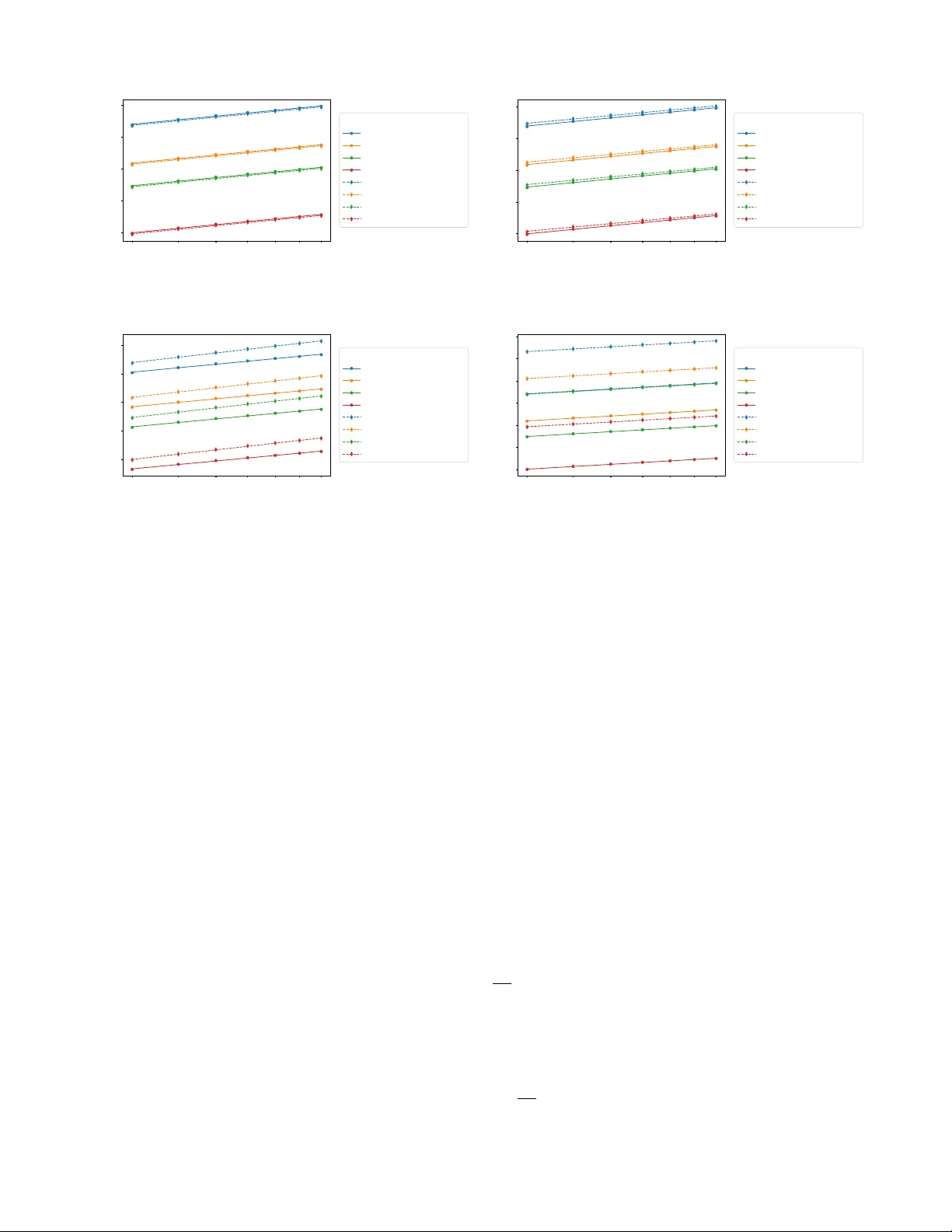
Lindbladian Sim ulation with Comm utator Bounds Xinzhao W ang 1 , 2 , ∗ Sh uo Zhou 1 , 2 , 5 , ∗ Xiao yang W ang 3 , 4 , Yi-Cong Zheng 5 , Shengyu Zhang 5 , † and T ongyang Li 1 , 2 ‡ 1 Center on F r ontiers of Computing Studies, Peking University, Beijing 100871, China 2 Scho ol of Computer Scienc e, Peking University, Beijing 100871, China 3 RIKEN Center for Inter disciplinary The or etic al and Mathematic al Scienc es (iTHEMS), Wako, Saitama 351-0198, Jap an 4 RIKEN Center for Computational Scienc e (R-CCS), Kob e, Hyo go 650-0047, Jap an and 5 T enc ent Quantum L ab or atory, T enc ent, Shenzhen, Guangdong 518057, China (Dated: March 31, 2026) T rotter decomposition pro vides a simple approac h to sim ulating op en quan tum systems b y decom- p osing the Lindbladian in to a sum of individual terms. While it is established that T rotter errors in Hamiltonian sim ulation depend on nested comm utators of the summands, such a relationship remains po orly understo od for Lindbladian dynamics. In this Letter, w e deriv e comm utator-based T rotter error b ounds for Lindbladian simulation, yielding an O ( √ N ) scaling in the num b er of T rot- ter steps for lo cally interacting systems on N sites. When estimating observ able av erages, w e apply Ric hardson extrap olation to achiev e p olylogarithmic precision while main taining the comm utator scaling. T o b ound the extrapolation remainder, w e develop a general truncation b ound for the Bak er-Campb ell-Hausdorﬀ expansion that b ypasses common conv ergence issues in physically rel- ev an t systems. F or lo cal Lindbladians, our results demonstrate that the T rotter-based methods outp erform prior simulation tec hniques in system-size scaling while requiring only O (1) ancillas. Numerical simulations further v alidate the predicted system-size and precision scaling. In tro duction — The Lindblad master equation serves as the canonical framework for the study of op en quan- tum systems [ 1 , 2 ]. It has b een used to mo del dissipa- tiv e pro cesses across diverse ﬁelds, ranging from quantum optics [ 3 , 4 ] and quan tum statistical mechanics [ 5 , 6 ] to noise mo deling in quan tum computation [ 7 ]. B ey ond de- scribing ph ysical phenomena, Lindblad dynamics is ap- plied to design quan tum algorithms for the dissipativ e preparation of a wide v ariet y of quantum states [ 8 ], in- cluding thermal states [ 9 ], ground states [ 10 ], and excited states [ 11 ]. F urthermore, it extends to solving diﬀeren tial equations [ 12 ] and optimization problems [ 13 , 14 ]. Eﬃcien t sim ulation of Lindblad dynamics is therefore essen tial, serving both as a to ol to in vestigate op en quan- tum system dynamics and as a primitiv e for executing suc h quan tum algorithms. Digital simulation of Lind- blad dynamics was initiated using T rotter decomposi- tion [ 15 , 16 ]. These methods appro ximate the ev olu- tion e t L generated b y a Lindbladian L = P m j =1 L j us- ing a pro duct formula—a pro duct of the exponentials of the summands. Since then, v arious algorithmic tec h- niques hav e b een dev elop ed [ 17 – 26 ]. In particular, meth- o ds based on linear combinations of unitaries [ 9 , 27 – 29 ] ac hieve near-optimal complexit y in terms of ev olution time and precision. How ev er, they require substantial an- cilla ov erhead and complex m ulti-qubit controlled op er- ations. In contrast, T rotter-based methods require fewer ancillas and simpler circuits [ 25 ], making them more suit- able for practical implemen tation. ∗ Equal Con tribution. † Corresponding author. Email: shengyzhang@tencent.com ‡ Corresponding author. Email: tongyangli@pku.edu.cn Bey ond hardware eﬃciency , T rotter-based metho ds of- fer a distinct adv an tage in Hamiltonian sim ulation: the error is go verned by nested comm utators rather than the sum of the norms of the operator summands, en- abling tigh ter complexit y b ounds [ 30 ]. Ho wev er, analo- gous comm utator bounds are largely missing for Lindbla- dian simulation. Existing analyses b ound the error using the sum of the norms P m j =1 ∥L j ∥ , which fail to accoun t for the Lie-algebraic structure of the nested com m utators of {L j } . Deriving suc h b ounds is diﬃcult, as standard comm utator-based T rotter error representation inv olves in verse time evolutions [ 30 ]. F or Lindbladians, the norms of these terms can grow exp onen tially due to dissipation. In this Letter, we provide the ﬁrst commutator-based error b ounds for Lindbladian pro duct form ulas, ad- dressing b oth the total T rotter error and its arbitrarily high-order remainders. The b ound for the total error implies that standard pro duct form ulas with a ﬁxed step size ac hieve a complexity scaling gov erned by nested comm utators of the op erator summands. T o ac hieve higher precision, we use Ric hardson extrap- olation to eliminate the leading-order terms of the T rotter error, such that the ﬁnal precision is deter- mined b y the high-order remainder. The b ound for the high-order remainders then leads to simulation algorithm with logarithmic precision while maintaining the comm utator-based scaling. Speciﬁcally , for lo cal Lindbladians on N sites, our approach requires only O ( √ N ) T rotter steps, which is a cubic improv emen t o ver previous analyses. F urthermore, the circuit im- plemen tation requires only constant ancillas, making it fa vorable for early fault-toleran t devices. In addition, we conduct numerical experiments to verify the scaling with system size and the error reduction from extrap olation. 2 Problem setup — W e aim to sim ulate open quan tum systems go verned by the Lindblad master equation: d ρ d t = L ( ρ ) : = − i[ H , ρ ] + m D X ν =1  L ν ρL † ν − 1 2 { L † ν L ν , ρ }  . While our T rotter error analysis holds for general Lind- bladians, we focus on systems deﬁned on a lattice [ N ] with k -lo cal coheren t terms and jump op erators. Specif- ically , we assume the Hamiltonian H = P m C µ =1 H µ and eac h jump op erator L ν = P γ d ν,γ are sums of at most Γ lo cal comp onen ts each supp orted on at most k sites. W e refer to such a system as a (Γ , k ) -lo c al Lindbladian . In this setting, the Lindbladian can b e expanded as a sum of sup erop erators L = P M v =1 K v , where each K v acts on at most 2 k sites. W e further assume the system is g - extensive , meaning that the lo cal interaction strength at eac h site is bounded by P v :supp( K v ) ∋ j ∥K v ∥ ⋄ ≤ g, ∀ j ∈ [ N ] , (1) where ∥ · ∥ ⋄ denotes the diamond norm and supp( · ) rep- resen ts the supp ort of the sup erop erator. In the sp ecial case where eac h jump op erator is individually supp orted on at most k sites, the (1 , k )-local Lindbladian reduces to the standard deﬁnition of a k -lo c al Lindbladian . W e consider t wo tasks: (i) approximating the ev olu- tion channel e t L within a diamond-norm error ε , and (ii) estimating the exp ectation v alue of a given observ able O with an additiv e error ε ∥ O ∥ for the time-ev olv ed state. T rotter error analysis — W e ﬁrst deriv e T rotter error b ounds for general Lindbladians, whic h determine the n umber of T rotter steps required for a target precision. W e consider the second-order pro duct form ula S ( t ) : = 1 Y j = m e t L j / 2 m Y j =1 e t L j / 2 , (2) based on a decomp osition L = P m j =1 L j with m := m C + m D summands. Each Lindbladian summand L j represen ts either a coherent term H µ ( · ) = − i[ H µ , · ] or a dissipator D ν ( · ) = L ν ( · ) L † ν − 1 2 { L † ν L ν , ·} . W e focus on the second-order pro duct form ula as it oﬀers better er- ror scaling compared to the ﬁrst-order case while av oid- ing the negativ e-time ev olution required b y higher-order T rotter-Suzuki decompositions [ 31 ] that are not experi- men tally feasible. T rotter errors in Hamiltonian simulation are often ex- pressed as right-nested comm utators of the op erator sum- mands [ 30 ]. A right-nested commutator of {L j } is deﬁned as [ L j 1 , . . . , L j q ] : = [ L j 1 , [ L j 2 , . . . , [ L j q − 1 , L j q ] . . . ]]. The n umber of operators q is called the gr ade of the commu- tator. W e giv e new bounds on T rotter error and its higher- order remainders in Lindbladian sim ulation using the Lindbladian sim ulation via second-order T rotterization Channel appro ximation Observ able estimation Direct pro duct formula Theorem 1 Commutator b ounds for T rotter error T rotter depth O ( √ N ε − 1 / 2 ) BCH truncation bound Theorem 2 Bypasses BCH div ergence Ric hardson extrap olation Theorem 3 Commutator b ounds and exp onen tially improv ed precision T rotter depth O ( √ N polylog( N /ε )) Circuit implemen tation of T rotter steps Stinespring dilation k -lo cal Lindbladians O (1) ancillas Blo ck enco ding (Γ , k )-lo cal Lindbladians polylog ancillas FIG. 1: Flo w chart of our simulation framew ork. sum of the norms of doubly right-neste d c ommutators de- noted b y α ( q 1 ,...,q d ) comm ( L 1 , . . . , L m ), or α ( q 1 ,...,q d ) comm for short: X j 1 , 1 ,...,j d,q d    [ L j 1 , 1 , . . . , L j 1 ,q 1 ] , . . . , [ L j d, 1 , . . . , L j d,q d ]    ⋄ . This quan tity represents the sum ov er all right-nested comm utators of righ t-nested commutators of the op era- tor summands with grades q 1 , . . . , q d resp ectiv ely . Channel approximation. — F or approximating the ev olution c hannel e t L , w e giv e a comm utator bound anal- ogous to Hamiltonian simulation. W e decomp ose the to- tal time t into r segmen ts of duration τ = t/r and ap- pro ximate the evolution as S ( τ ) r . Due to the con tractiv- it y of Lindbladian evolution, i.e., ∥ e τ L ∥ ⋄ = 1 for τ ≥ 0, the total simulation error is bounded b y the sum of one- step T rotter errors r ∥S ( τ ) − e τ L ∥ ⋄ . T rotter error b ounds for general non-an ti-Hermitian generators can gro w ex- p onen tially with time [ 30 ]. This growth typically arises from terms in the T rotter error that lac k contractivit y , suc h as the in v erse ev olutions e − τ L . How ev er, we observe that these non-con tractiv e terms cancel out in our case (see Appendix B for a detailed deriv ation). This ensures the one-step T rotter error grows only p olynomially with time τ : ∥S ( τ ) − e τ L ∥ ⋄ ≤ α (3) comm τ 3 , (3) where α (3) comm is the sum of all grade-3 righ t-nested com- m utators [ 32 ]. T o ensure the simulation error is b ounded 3 b y ε , we set r to satisfy r · α (3) comm ( t/r ) 3 ≤ ε . This yields the follo wing requiremen t for the T rotter n um b er. Theorem 1 (Channel appro ximation) . F or any evolu- tion time t > 0 and pr e cision ε > 0 , the Lindbladian evolution e t L c an b e appr oximate d to pr e cision ε in the diamond norm using r = O  ( α (3) comm ) 1 / 2 t 3 / 2 / √ ε  (4) steps of the se c ond-or der pr o duct formula ( 2 ). F or a (Γ , k )-local and g -extensive Lindbladian L on [ N ], standard T rotter error b ounds [ 16 ] depend on the total interaction strength, whic h is b ounded by summing Eq. ( 1 ) o v er all sites: P v ∥K v ∥ ⋄ ≤ P N j =1 P v :supp( K v ) ∋ j ∥K v ∥ ≤ N g . (5) This leads to a T rotter n umber r = O ( N 3 / 2 ( g t ) 3 / 2 ϵ − 1 / 2 ). In con trast, our comm utator-based estimate α (3) comm = O ( k 2 g 3 N ) (6) yields r = O ( √ N k ( g t ) 3 / 2 ϵ − 1 / 2 ). This provides a factor- of- N reduction in the num ber of T rotter steps, oﬀering a signiﬁcan t adv antage for large-scale simulations ( k ≪ N ). Observ able estimation. — F or the task of estimating the exp ectation v alue T r[ O e t L ρ 0 ], a direct T rotter im- plemen tation requires O (1 / √ ε ) T rotter depth to reach a bias ε by Theorem 1 . T o impro ve this dep endence to p olylog(1 /ε ), several T rotter error mitigation tec hniques based on extrap olation [ 33 , 34 ] and interpolation [ 35 ] ha ve been developed for Hamiltonian simulation. Recent w ork also uses extrap olation to mitigate Hamiltonian di- lation errors in Lindbladian sim ulation [ 28 ]. In this Let- ter, we use extrap olation to suppress the T rotter error in Lindbladian simulation, achieving a p olylog(1 /ε ) T rot- ter depth while preserving the commutator complexit y scaling. W e deﬁne the step-size-dep enden t exp ectation v alue f ( s ) : = T r[ O S ( st ) 1 /s ρ 0 ] and apply Ric hardson ex- trap olation [ 36 ] to estimate the zero-step-size limit lim s → 0 f ( s ) = T r[ O e t L ρ 0 ]. Since f ( s ) is an ev en func- tion for symmetric pro duct formulas, ev aluating it at p distinct step sizes { s j } p j =1 allo ws us to cancel the ﬁrst p − 1 leading error terms, with the resulting ex- trap olation error gov erned b y the 2 p -th order remainder R 2 p ( s ) = O ( s 2 p ). T o b ound this remainder, a standard approac h is to apply the BCH formula to the pro duct form ula, yielding S ( st ) = exp  P ∞ q =1 Φ q ( st ) q  , and then expand the exponential exp  P ∞ q =1 Φ q ( st ) q /s  , the expo- nen tial S ( st ) 1 /s in f ( s ) [ 34 , 37 , 38 ]. Here Φ q is a w eigh ted sum of grade- q righ t-nested commutators of the op erator summands and is bounded by ∥ Φ q ∥ ⋄ ≤ α ( q ) comm /q 2 [ 39 ]. This approach assumes the con vergence of the BCH series P ∞ q =1 Φ q ( st ) q . How ever, for local lattice systems, the nested commutator b ound α ( q ) comm can grow as O ( q !) (see [ 38 , Lemma 7]), which preven ts a proof of the con- v ergence for any ﬁxed step size s > 0. Suc h a blow-up of high-order BCH terms has also b een observed in quan- tum chemistry [ 40 ]. T o bypass this diﬃculty , Mizuta [ 38 ] sho wed that the exp onential of the truncated BCH ex- pansion exp  P q 0 q =1 Φ q ( st ) q  appro ximates the pro duct form ula S ( st ) if each L j is a sum of mutually comm uting lo cal Hermitian operators. How ev er, this condition do es not hold for most practical Lindbladians. Here, we give a general b ound for the BCH truncation error in terms of the doubly right-nested comm utators b ound α ( q 1 ,...,q d ) comm . Theorem 2 (BCH truncation error bound) . Deﬁne α comm ,q 0 ( st ) = ∞ X d =1 1 d ! X 1 ≤ q 1 ,...,q d ≤ q 0 q 1 + ··· + q d ≥ q 0 +1 α ( q 1 ,...,q d ) comm ( st ) q 1 + ··· + q d . If α comm ,q 0 ( st ) ≤ 1 , the trunc ation err or of the q 0 -th or- der BCH exp ansion for the pr o duct formula S ( st ) satis- ﬁes   exp  P q 0 q =1 Φ q ( st ) q  − S ( st )   ⋄ ≤ eα comm ,q 0 ( st ) . Though seemingly intricate, the b ound can b e con- trolled to remain small for lo cal Lindbladians, as w e will demonstrate following Theorem 3 . T o establish the b ound, we map the discrete product form ula to a con- tin uous ev olution Y ( τ ) generated by a piecewise con- stan t Lindbladian L ( τ ) prop ortional to the step size st . The Magnus expansion represents the ev olution op er- ator as Y ( τ ) = exp  P ∞ q =1 Ω q ( τ )  , where eac h Ω q ( τ ) is an integrated righ t-nested comm utator of L ( τ ). Let Y ( q 0 ) ( τ ) := exp  Ω ( q 0 ) ( τ )  b e the exp onen tial of the trun- cated Magnus expansion Ω ( q 0 ) := P q 0 q =1 Ω q ( τ ). By the deriv ative form ula for the exp onen tial map, Y ( q 0 ) ( τ ) is generated b y L ( q 0 ) ( τ ) = ∞ X ℓ =0 1 ( ℓ + 1)! ad ℓ Ω ( q 0 ) ( τ ) ( ˙ Ω ( q 0 ) ( τ )) . (7) The BCH truncation error is then b ounded by the inte- grated generator diﬀerence ∥L ( τ ) − L ( q 0 ) ( τ ) ∥ ⋄ . F ollowing the order conditions prov ed in Ref. [ 41 ], L ( q 0 ) ( τ ) matches L ( τ ) up to order q 0 . Consequently , the low er-order terms in the expansion of Eq. ( 7 ) cancel out. The b ound α comm ,q 0 ( st ) then naturally emerges when we b ound the remaining terms with order greater than q 0 , which are comp osed of righ t-nested comm utators of Ω q and ˙ Ω q , cre- ating a doubly righ t-nested commutator structure. W e refer to Appendix C for a detailed deriv ation. Giv en a truncation order q 0 , the extrap olation remain- der R 2 p ( s ) can b e decomp osed into tw o parts. The ﬁrst is the remainder of the p o w er series expansion of the truncated exponential exp  P q 0 q =1 Φ q ( st ) q /s  , which is O  (max q ≤ q 0 ( α ( q ) comm ) 1 /q t ) 3 p s 2 p  dep ending only on the 4 ﬁnite sequence { α ( q ) comm } q ≤ q 0 . The second is the BCH truncation error, whic h scales as O ( α comm ,q 0 ( st ) /s ) when accum ulated ov er 1 /s steps. By choosing a step size s = O ((max q ≤ q 0 ( α ( q ) comm ) 1 /q t ) − 3 / 2 ), the ﬁrst part is sup- pressed exp onen tially in the extrap olation order p , such that p = O (log(1 /ε )) suﬃces to reach precision ε . Pro- vided that the BCH truncation error remains suﬃciently small—a condition w e verify below for (Γ , k )-local Lind- bladians—w e obtain the follo wing theorem. Theorem 3 (Observ able estimation via extrap olation) . L et t > 0 b e the simulation time and ε ∈ (0 , 1) b e the pr e cision. Given a BCH trunc ation or der q 0 , by cho osing an extr ap olation or der p = O (log(1 /ε )) and the maxi- mum step size, which s p satisﬁes s p = O  max q ≤ q 0 ( α ( q ) comm ) 1 q t  − 3 2  , α comm ,q 0 ( s p t ) = O  s p ε log p  , the extr ap olation algorithm estimates the exp e ctation value tr  O e t L ρ 0  to pr e cision ε ∥ O ∥ using e O (1 /ε 2 ) [ 42 ] cir cuit runs, e ach c onsisting of at most e O (1 /s p ) T r otter steps. F or any (Γ , k )-local and g -extensiv e Lindbladian L on [ N ], we show that the doubly right-nested com- m utator b ound scales as α ( q 1 ,...,q d ) comm = O (( q 0 k g ) q q d N ) for q 1 , . . . , q d ≤ q 0 , where q = P d j =1 q j . The proof of this scaling and its application to the BCH trunca- tion error are detailed in App endix D 1 . Speciﬁcally , w e hav e eα comm ,q 0 ( st ) ≤ N e − q 0 for any step size st = O (( q 0 k g ) − 1 ). Applying these estimates to Theorem 3 yields a step size s p = e O ( N − 1 / 2 ( k gt ) − 3 / 2 ) satisfying all the requiremen ts. Therefore, estimating the observ able tr  O e t L ρ 0  to precision ϵ ∥ O ∥ requires e O ( ϵ − 2 ) circuit runs, each consisting of e O ( √ N ( k g t ) 3 / 2 ) T rotter steps, which sim ultaneously achiev es p olylog(1 /ϵ ) preci- sion and e O ( √ N ) system-size scaling. Circuit implemen tation — W e consider tw o im- plemen tation strategies for the T rotter step S ( st ). First, for k -lo cal Lindbladians with k = O (1) where eac h L j is supported on k qubits, the c hannel exp( st L j ) can b e implemen ted via Stinespring dilation as a unitary U j acting on k qubits with 2 k ancillas. Since U j requires e O (1) elemen tary gates via the Solo v ay-Kitaev algorithm, eac h T rotter step S ( st ) can b e executed using e O ( m ) gates. Therefore, the gate complexity p er circuit run is e O ( m √ N ( g t ) 3 / 2 ε − 1 / 2 ) for c hannel appro ximation and e O ( m √ N ( g t ) 3 / 2 ) for observ able estimation. Second, for (Γ , k )-Lindbladians where eac h jump op- erator L ν is decomp osed into at most Γ commp o- nen ts { d ν,γ } γ eac h supp orted on k = O (1) sites, w e ass u me query access to the blo c k enco dings of the Hamiltonian terms H µ and the comp onen ts d ν,γ . Then, the evolution e τ L j can b e implemented using e O (max { τ Γ ∥L j ∥ be , 1 } ) queries and gates [ 28 ], where T ABLE I: Complexity and ancilla requirements for (Γ , O (1))-lo cal Lindbladian simulation. The top and b ottom sections denote channel approximation and observ able estimation, resp ectiv ely . All observ able estimation methods require e O (1 /ϵ 2 ) circuit runs. Sc heme Complexit y per circuit run Ancilla LCU [ 28 , 29 ] e O ( m Γ N g t ) polylog ( m Γ N g t/ε ) q -order DH [ 22 ] O (( m Γ) q N g t ( t/ε ) 1 /q ) Ω( q log m ) Ours ( Γ = 1 ) e O ( m √ N ( g t ) 3 / 2 ε − 1 / 2 ) O (1) LCS [ 25 ] e O ( m Γ( N g t ) 2 ) 2 RD [ 23 ] e O (Γ( N g t ) 2 ) O (log Γ) Ours ( Γ = 1 ) e O ( m √ N ( g t ) 3 / 2 ) O (1) Ours e O (Γ N g t + m Γ √ N ( g t ) 3 / 2 ) p olylog( m Γ N g t/ε ) ∥L j ∥ be denotes the sum of the norms of the lo cal comp o- nen ts within L j . One T rotter step S ( st ) thus requires e O ( P m j =1 Γ max { τ ∥L j ∥ be , 1 } ) = e O (Γ( τ ∥L∥ be + m )) = e O (Γ( τ N g + m )) queries and gates, where w e b ound ∥L∥ be using Eq. ( 5 ). Multiplying this by the total n umber of steps, we obtain a total complexity of e O (Γ N g t + m Γ √ N ( g t ) 3 / 2 ) p er circuit run for observ able estimation. The resulting complexity is compared in T able I . F or t ypical lo cally in teracting mo dels where m = O ( N ), our analysis achiev es a e O ( N 3 / 2 ) scaling, impro ving the state-of-the-art b y a factor of √ N . Numerical demonstration — W e conduct nu- merical simulations to supp ort our theoretical ﬁndings. Sp eciﬁcally , w e consider an N -qubit 1D transverse- ﬁeld Ising mo del with single-qubit dissipation. The system Hamiltonian is decomp osesd into tw o parts H = H X + H Z : where H X = − J N − 1 X j =1 X j X j +1 , H Z = − h N X j =1 Z j . Eac h jump operator acts on a single qubit in the following form, where γ is the coupling strength, L ν = √ γ | 0 ⟩ ν ⟨ 1 | ν , ν = 1 , . . . , N . F or c hannel appro ximation, w e quan tify the sim ulation error using the trace distance ∥ ( e t L − S ( t/r ) r ) ρ 0 ∥ 1 , whic h lo wer-bounds the worst-case diamond distance. The ex- act ev olution is computed via high-precision numerical in tegration. F or observ able estimation, we compute the total magnetization T r[ O S ( t/r ) r ρ 0 ] with O = P N j =1 Z j , ﬁxing J = 1 . 0, h = 0 . 5, and t = 0 . 2. While we fo cus on the initial state ρ 0 = | 1 N ⟩⟨ 1 N | in the main text, results for other initial states—including | 0 N ⟩⟨ 0 N | , | + N ⟩⟨ + N | , and I / 2 N —along with further n umerical details, are pro- vided in Appendix E . Commutator Sc aling. W e ﬁrst verify the O ( N ) com- m utator scaling of the T rotter error in Eq. ( 3 ), as pre- dicted for local Lindbladians via Eq. ( 6 ). As shown in 5 4 5 6 7 8 9 10 qubit number N − 3 . 5 − 3 . 0 − 2 . 5 − 2 . 0 − 1 . 5 lg k ( e t L − S ( t/r ) r ) ρ 0 k 1 Lindbladian simulation error vs. system size N ρ 0 = | 1 N ih 1 N | γ = 0 . 1, r = 1, slope=0.721 γ = 0 . 1, r = 2, slope=0.721 γ = 0 . 1, r = 3, slope=0.720 γ = 0 . 1, r = 7, slope=0.721 γ = 1 . 0, r = 1, slope=0.689 γ = 1 . 0, r = 2, slope=0.686 γ = 1 . 0, r = 3, slope=0.685 γ = 1 . 0, r = 7, slope=0.684 FIG. 2: T rotter error for Lindbladian sim ulation v ersus system size N . The initial state ρ 0 = | 1 N ⟩⟨ 1 N | . The data points are plotted on a log-log scale and ﬁtted by linear regression. The solid lines with circle markers denote coupling strength γ = 0 . 1, whereas the dashed lines with diamond mark ers denote γ = 1 . 0. W e distinguish the T rotter step r by the color of the lines. Figure 2 , we plot the sim ulation error v ersus qubit num- b er N ∈ [4 , 10] on a log-log scale, and the data p oin ts ﬁt w ell with linear regression. W e can observe that for coupling strength γ = 0 . 1, the error scales with around O ( N 0 . 72 ) regardless of the T rotter num ber r , consisten t with Eq. ( 6 ). Similarly , for γ = 1 . 0, the errors with four diﬀeren t r all scale with around O ( N 0 . 69 ). Other ini- tial states presented in App endix E ha v e the largest er- ror scaling of O ( N 0 . 96 ). All observed n umerical scalings are smaller than O ( N ), demonstrating that the empirical p erformance satisﬁes the theoretically predicted commu- tator scaling. R ichar dson Extr ap olation. W e next verify the sup- pression of T rotter bias via Richardson extrap olation. T o ac hiev e the high precision required to v erify higher- order scalings, we simulate a small system ( N = 5) whose evolution channels can b e computed directly via sup erop erator exp onen tials. As sho wn in Figure 3 , after extrap olation with p = 3 step sizes, the errors decrease by several orders of magnitude. The errors scales approximately as O ( r − 6 scale ), consistent with the predicted 2 p -th order extrap olation remainder for p = 3. 1 2 3 4 5 6 7 8 9 r scale − 7 − 6 − 5 − 4 − 3 − 2 − 1 lg | T r[ O S ( t/r ) r ρ 0 ] − T r[ Oe t L ρ 0 ] | T rotter error scaling with Richardson extrap olation N = 5, ρ 0 = | 1 N ih 1 N | γ = 0 . 1, original, slop e= − 1 . 995 γ = 1 . 0, original, slop e= − 1 . 970 γ = 0 . 1, extrap., slop e= − 6 . 187 γ = 1 . 0, extrap., slop e= − 5 . 662 FIG. 3: Error scaling of observ able exp ectations with and without Ric hardson extrapolation ( N = 5). The orange lines denote ra w T rotter errors with r = 4 r scale , whereas the blue lines represen t extrapolated results using r ∈ { r scale , 2 r scale , 4 r scale } with linear com bination co eﬃcien ts { 1 45 , − 4 9 , 64 45 } . The solid and dashed lines corresp ond to diﬀerent coupling strengths γ . Discussion — In this Letter, we analyze t w o T rotter- based quan tum algorithms for Lindbladian simulation and show that their complexities scale with the nested comm utators of the operator summands. The ﬁrst ap- pro ximates the time-ev olution channel within a small di- amond distance, while the second estimates observ able a verages with logarithmic precision scaling via Ric hard- son extrap olation. T o derive these commutator b ounds, w e dev elop a general truncation b ound for the BCH ex- pansion that b ypasses common con v ergence issues in an- alyzing high-precision T rotter metho ds for both open and closed systems [ 34 , 37 , 38 , 43 ]. Our analysis shows that pro duct form ulas achiev e improv ed system-size complex- it y scaling for simulating locally interacting Lindbladi- ans relative to prior b ounds. While w e use tw o sp eciﬁc circuit implementations as examples, the T rotter error b ounds are independent of these details. This suggests that the cost p er T rotter step could b e further reduced using metho ds tailored to speciﬁc systems. Finally , w e conduct n umerical sim ulations to v alidate our theory . Ac kno wledgements — Xinzhao W ang, Sh uo Zhou, and T ongyang Li are supp orted by the National Natural Sci- ence F oundation of China (Gran t Numbers 62372006 and 92365117). Xiaoy ang W ang is supp orted by the RIKEN TRIP initiativ e (RIKEN Quantum) and the UT okyo Quan tum Initiative. 6 App endix A: Preliminaries 1. Magn us expansion Consider a time-dependent linear diﬀeren tial equation d Y ( t ) d t = A ( t ) Y ( t ) , Y (0) = I . The Magus expansion expresses Y ( t ) as the exp onen tial of a time-dep enden t op erator Y ( t ) = exp(Ω( t )), where the exp onen t Ω( t ) admits a series expansion [ 44 ] Ω( t ) = ∞ X q =1 Ω q ( t ) . The p -th order Magn us expansion is denoted by Ω ( p ) = p X q =1 Ω q . (A1) Eac h Ω q ( t ) can be written as an integral of nested commutators of A ( t ): Ω q ( t ) = X σ ∈ S q c σ,q Z t 0 d τ 1 Z τ 1 0 d τ 2 · · · Z τ q − 1 0 d τ q R σ  [ A ( τ 1 ) , A ( τ 2 ) , . . . , A ( τ q )]  , (A2) where S q denotes the set of permutations of [ q ], c σ,q = 1 q 2 ( − 1) d σ  q − 1 d σ  (A3) satisfying | c σ,q | ≤ 1 /q 2 , and d σ denotes the n umber of i ∈ [ q − 1] such that σ ( i ) > σ ( i + 1) [ 45 ]. The deriv ative of Ω q ( t ) is ˙ Ω q ( t ) = X σ ∈ S q c σ,q Z t 0 d τ 2 Z τ 2 0 d τ 3 · · · Z τ q − 1 0 d τ q R σ  [ A ( t ) , A ( τ 2 ) , . . . , A ( τ q )]  . (A4) 2. Ric hardson extrap olation Lemma 1 (see [ 34 , Lemma 5]) . L et f ( x ) ∈ C 2 p +2 ([ − 1 , 1]) b e an even function, and let Q j and R j b e a de gr e e- ( j − 1) T aylor p olynomial and T aylor r emainder, r esp e ctively, such that f ( x ) = Q j ( x ) + R j ( x ) . L et F ( p ) ( s ) b e the p -th or der R ichar dson extr ap olation of f ( x ) at p oints s j = s/r j for j ∈ [ p ] , deﬁne d as F ( p ) ( s ) = p X j =1 b j f ( s j ) , wher e the r ep etition numb ers r j and c o eﬃcients b j ar e given by r j = & √ 8 p π sin( π (2 j − 1) / 8 p ) ' , b j = Y ℓ  = j 1 1 − r 2 ℓ /r 2 j . Then, the extr ap olation err or satisﬁes | F ( p ) ( s ) − f (0) | ≤ ∥ b ∥ 1 max j ∈ [ p ] | R 2 p ( s j ) | , wher e ∥ b ∥ 1 ≤ C log p for some absolute c onstant C > 0 . 7 3. T ec hnical lemmas Let A ( τ ) and B ( τ ) b e tw o contin uous op erator-v alued functions. W e rely on the follo wing lemma to decompose the time-ordered exp onen tial of the sum A ( τ ) + B ( τ ). This result is essentially the interaction picture representation of the ev olution. Lemma 2 ([ 46 , P age 21]) . L et H ( τ ) = A ( τ ) + B ( τ ) b e an op er ator-value d function deﬁne d for τ ∈ R with c ontinuous summands A ( τ ) and B ( τ ) . Then exp T  Z t 0 H ( τ ) d τ  = exp T  Z t 0 A ( τ ) d τ  · exp T  Z t 0 exp − 1 T  Z τ 1 0 A ( τ 2 ) d τ 2  B ( τ 1 ) exp T  Z τ 1 0 A ( τ 2 ) d τ 2  d τ 1  . W e use the following lemma to b ound the diﬀerence betw een pow ers of a superop erator and a quantum c hannel. Lemma 3. L et N 1 , N 2 b e t wo sup er op er ators, wher e N 1 is a quantum channel. F or any p ositive inte ger k , the diﬀer enc e b etwe en N k 1 and N k 2 c an b e b ounde d by ∥N k 1 − N k 2 ∥ ⋄ ≤ k max { 1 , ∥N 2 ∥ ⋄ } k − 1 ∥N 1 − N 2 ∥ ⋄ . Pr o of. W e use the telescoping sum iden tit y for the diﬀerence betw een pow ers of t w o op erators: N k 1 − N k 2 = k − 1 X j =0 N k − 1 − j 1 ( N 1 − N 2 ) N j 2 . T aking the diamond norm on b oth sides, we obtain ∥N k 1 − N k 2 ∥ ⋄ ≤ k − 1 X j =0 ∥N 1 ∥ k − 1 − j ⋄ ∥N 1 − N 2 ∥ ⋄ ∥N 2 ∥ j ⋄ = ∥N 1 − N 2 ∥ ⋄ k − 1 X j =0 ∥N 2 ∥ j ⋄ ≤ k max { 1 , ∥N 2 ∥ ⋄ } k − 1 ∥N 1 − N 2 ∥ ⋄ , where the second line follo ws from the fact that N 1 is a quan tum c hannel, so ∥N 1 ∥ ⋄ = 1. App endix B: Commutator b ounds for the pro duct formula of Lindbladians In this section, we deriv e commutator-based error b ounds for the ﬁrst- and second-order pro duct form ulas of Lindbladians. The follo wing theorem establishes the bound for the second-order case. Theorem 4. L et L = P m j =1 L j b e a Lindbladian c onsisting of m summands and let t > 0 . L et S ( t ) = Q 1 j = m e t L j / 2 Q m j =1 e t L j / 2 b e the se c ond-or der pr o duct formula. The additive T r otter err or is b ounde d by ∥S ( t ) − e t L ∥ ⋄ ≤ t 3 12 m X j 1 =1      m X j 3 = j 1 +1 L j 3 , m X j 2 = j 1 +1 L j 2 , L j 1      ⋄ + t 3 24 m X j 1 =1      L j 1 , L j 1 , m X j 2 = j 1 +1 L j 2      ⋄ Pr o of. The pro of generalize the deriv ation in [ 30 , App endix L] from Hamiltonians to Lindbladians. W e ﬁrst consider the m = 2 case. F ollowing [ 30 , Eq. (L4)], the additiv e T rotter error can be expressed as ∥ e t L 1 / 2 e t L 2 e t L 1 / 2 − e t ( L 1 + L 2 ) ∥ ⋄ = Z t 0 d τ 1 Z τ 1 0 d τ 2 Z τ 2 0 d τ 3 e ( t − τ 1 ) L e τ 1 L 1 / 2 h e τ 3 ad L 2 ad 2 L 2  L 1 2  + e − τ 3 ad L 1 / 2 ad 2 −L 1 / 2 ( L 2 ) i e τ 1 L 2 e τ 1 L 1 / 2 . Observ e that the only Lindbldian evolution with negative time in the expression is the e − τ 3 L 1 / 2 arising from e − τ 3 ad L 2 / 2 . Com bining it with the preceding term e τ 1 L 1 / 2 giv es e ( τ 1 − τ 3 ) L 1 / 2 , and the evolution time ( τ 1 − τ 3 ) / 2 is non-negative 8 since τ 3 ≤ τ 2 ≤ τ 1 . Therefore, since ∥ e t L ′ ∥ ⋄ = 1 for any Lindbladian L ′ and t ≥ 0, the diamond norm of the additive T rotter error can b e bounded by ∥ e t L 1 / 2 e t L 2 e t L 1 / 2 − e t ( L 1 + L 2 ) ∥ ⋄ ≤ Z t 0 d τ 1 Z τ 1 0 d τ 2 Z τ 2 0 d τ 3     ad 2 L 2  L 1 2     ⋄ +   ad 2 −L 1 / 2 ( L 2 )   ⋄  = Z t 0 d τ 1 Z τ 1 0 d τ 2 Z τ 2 0 d τ 3  1 2 ∥ [ L 2 , L 2 , L 1 ] ∥ ⋄ + 1 4 ∥ [ L 1 , L 1 , L 2 ] ∥ ⋄  = t 3 12 ∥ [ L 2 , L 2 , L 1 ] ∥ ⋄ + t 3 24 ∥ [ L 1 , L 1 , L 2 ] ∥ ⋄ . F or a general Lindbladian L = P m j =1 L j , applying the triangle inequalit y via a telescoping sum argument giv es     1 Y j = m e t L j / 2 m Y j =1 e t L j / 2 − e t P m j =1 L j     ⋄ ≤ m X j 1 =1     1 Y j 2 = j 1 e t L j 2 / 2 e t P m j 2 = j 1 +1 L j 2 j 1 Y j 2 =1 e t L j 2 / 2 − 1 Y j 2 = j 1 − 1 e t L j 2 / 2 e t P m j 2 = j 1 L j 2 j 1 − 1 Y j 2 =1 e t L j 2 / 2     ⋄ ≤ m X j 1 =1     e t L j 1 / 2 e t P m j 2 = j 1 +1 L j 2 e t L j 1 / 2 − e t P m j 2 = j 1 L j 2     ⋄ ≤ t 3 12 m X j 1 =1      m X j 3 = j 1 +1 L j 3 , m X j 2 = j 1 +1 L j 2 , L j 1      ⋄ + t 3 24 m X j 1 =1      L j 1 , L j 1 , m X j 2 = j 1 +1 L j 2      ⋄ , where the last inequalit y follo ws from the T rotter error b ound derived abov e for the m = 2 case. This error bound leads to the following requirement on the T rotter num ber to achiev e a target precision ε Corollary 1. F or any evolution time t > 0 and tar get pr e cision ε > 0 , the Lindbladian evolution e t L c an b e appr oxi- mate d to pr e cision ε in the diamond norm using r steps of the se c ond-or der pr o duct formula S ( t/r ) , wher e r = O t 3 / 2 √ ε  m X j 1 =1      m X j 3 = j 1 +1 L j 3 , m X j 2 = j 1 +1 L j 2 , L j 1      ⋄ + m X j 1 =1      L j 1 , L j 1 , m X j 2 = j 1 +1 L j 2      ⋄  1 / 2 ! . Pr o of. By the triangle inequality , the total approximation error is bounded by ∥S ( t/r ) r − e t L ∥ ⋄ ≤ r ∥S ( t/r ) − e t L /r ∥ ⋄ . Applying the bound from the preceding theorem with step size t/r yields a total error of O ( r ( t/r ) 3 ) = O ( t 3 /r 2 ). Equating this bound to ε gives the result. If L is a (Γ , k )-Lindbladian, w e ha v e m X j 1 =1      m X j 3 = j 1 +1 L j 3 , m X j 2 = j 1 +1 L j 2 , L j 1      ⋄ + m X j 1 =1      L j 1 , L j 1 , m X j 2 = j 1 +1 L j 2      ⋄ ≤ 2 m X j 1 ,j 2 ,j 3 =1      L j 3 , L j 2 , L j 1      ⋄ ≤ 2 M X v 1 ,v 2 ,v 3 =1      K v 3 , K v 2 , K v 1      ⋄ = O ( k 2 g 3 N ) , where the third line follows from decomp osing the Lindbladians {L j } in to local sup eroperators {K v } eac h supported on at most 2 k sites, and applying the triangle inequalit y . The last line follo ws from Corollary 2 . The n um b er of T rotter steps then equals r = O ( √ N k ( g t ) 3 / 2 ε − 1 / 2 ) . Similarly , for the ﬁrst-order case, we hav e the follo wing theorem. 9 Theorem 5. L et L = P m j =1 L j b e a Lindbladian c onsisting of m summands and let t > 0 . L et S 1 ( t ) = Q m j =1 e t L j b e the ﬁrst-or der Lie-T r otter formula. The additive T r otter err or is b ounde d by ∥S 1 ( t ) − e t L ∥ ⋄ ≤ t 2 2 m X j 1 =1      m X j 2 = j 1 +1 L j 2 , L j 1      ⋄ . Pr o of. The pro of generalizes the deriv ation in [ 30 , Eq. (117)] from Hamiltonians to Lindbladians. W e ﬁrst consider the m = 2 case. F ollowing [ 30 , Eq. (117)], the additiv e T rotter error can be expressed as ∥ e t L 2 e t L 1 − e t ( L 1 + L 2 ) ∥ ⋄ =     Z t 0 d τ 1 Z τ 1 0 d τ 2 e ( t − τ 1 ) L e τ 1 L 2 e − τ 2 ad L 2 ([ L 2 , L 1 ]) e τ 1 L 1     ⋄ . Expanding the adjoin t action e − τ 2 ad L 2 ([ L 2 , L 1 ]) = e − τ 2 L 2 [ L 2 , L 1 ] e τ 2 L 2 , the in tegrand becomes e ( t − τ 1 ) L e ( τ 1 − τ 2 ) L 2 [ L 2 , L 1 ] e τ 2 L 2 e τ 1 L 1 . Observ e that the only Lindbladian ev olution with negative time in the adjoint expansion, e − τ 2 L 2 , is absorbed by the preceding term e τ 1 L 2 , leaving e ( τ 1 − τ 2 ) L 2 . Since τ 2 ≤ τ 1 ≤ t , all the ev olution times t − τ 1 , τ 1 − τ 2 , τ 2 , and τ 1 are non-negativ e. Therefore, since ∥ e τ L ′ ∥ ⋄ = 1 for an y Lindbladian L ′ and τ ≥ 0, the diamond norm of the additiv e T rotter error can b e bounded by ∥ e t L 2 e t L 1 − e t ( L 1 + L 2 ) ∥ ⋄ ≤ Z t 0 d τ 1 Z τ 1 0 d τ 2 ∥ [ L 2 , L 1 ] ∥ ⋄ = t 2 2 ∥ [ L 2 , L 1 ] ∥ ⋄ . F or a general Lindbladian L = P m j =1 L j , applying the triangle inequalit y via a telescoping sum argument giv es     m Y j =1 e t L j − e t P m j =1 L j     ⋄ ≤ m X j 1 =1     e t P m j 2 = j 1 +1 L j 2 j 1 Y j 2 =1 e t L j 2 − e t P m j 2 = j 1 L j 2 j 1 − 1 Y j 2 =1 e t L j 2     ⋄ ≤ m X j 1 =1      e t P m j 2 = j 1 +1 L j 2 e t L j 1 − e t P m j 2 = j 1 L j 2  j 1 − 1 Y j 2 =1 e t L j 2     ⋄ ≤ m X j 1 =1     e t P m j 2 = j 1 +1 L j 2 e t L j 1 − e t ( P m j 2 = j 1 +1 L j 2 + L j 1 )     ⋄ ≤ t 2 2 m X j 1 =1      m X j 2 = j 1 +1 L j 2 , L j 1      ⋄ , where the last inequalit y follo ws from the T rotter error b ound derived abov e for the m = 2 case. In the subsequen t sections, we fo cus on the second-order product formula due to its better error scaling compared to the ﬁrst-order case. Nev ertheless, our analytical framework generalizes naturally to the ﬁrst-order formula. App endix C: T runcation error of the BCH formula Let L 1 , . . . , L M b e general Lindbladians. The BCH form ula of the product e L M · · · e L 2 e L 1 can be written as e L M · · · e L 2 e L 1 = exp ∞ X q =1 Φ q ! , (C1) where eac h Φ q is a sum of the weigh ted righ t-nested commutators of L j (see Arnal et al. [ 47 ]): Φ q = X p v ≥ 0 , p 1 + ··· + p M = q 1 p 1 ! · · · p M ! X σ ∈ S q c σ,q R σ { [ L M , . . . , L M | {z } p M , . . . , L 1 , . . . , L 1 | {z } p 1 ] } , (C2) 10 and c σ,q is the same coeﬃcient as in Eq. ( A3 ). Deﬁne the sum of the q -fold right-nested comm utator norms as α ( q ) comm = M X v 1 ,...,v q =1   [ L v 1 , . . . , L v q ]   ⋄ . (C3) The norm of Φ q can be b ounded b y ∥ Φ q ∥ ⋄ ≤ 1 q 2 α ( q ) comm , for any q ≥ 1 (see, e.g., [ 37 , Prop osition 5]). Consequently , the series expansion in Eq. ( C2 ) conv erges if there exist t wo constants J, C ≥ 0 suc h that sup q ≥ J α ( q ) comm ≤ C. (C4) A trivial bound for α ( q ) comm is α ( q ) comm ≤  2 M X v =1 ∥L v ∥ ⋄  q , (C5) b y ∥ [ A, B ] ∥ ⋄ ≤ 2 ∥ A ∥ ⋄ ∥ B ∥ ⋄ and the triangle inequality . The quantit y α ( q +1) comm also app ears in the complexity of q -th order T rotterization in Hamiltonian sim ulation [ 30 ], where each L v is an Hermitian op erator in the decomp osition of the sim ulated Hamiltonian. F or some ph ysical Hamiltonians, suc h as k -local Hamiltonians on a lattice of size N , where eac h L v can be decomp osed as a sum of terms acting nontrivially on at most k sites, α ( q ) comm admits a sharper b ound than Eq. ( C5 ). This leads to the commutator scaling of the q -th order T rotterization. Sp eciﬁcally , supp ose that the maxim um interaction strength of P M v =1 L v on each site is g . Eq. ( C5 ) yields (2 N g ) q , while the b ound considering the comm utator structure of L v giv es N q !(2 k g ) q = O ( N ( qk g ) q ). The latter b ound provides a b etter complexity scaling for local Hamiltonians where k ≪ N and q is constan t. Ho wev er, in the error analysis of adv anced T rotter methods aiming for high precision [ 34 , 37 ], b ounds on α ( q ) comm for a single q are insuﬃcient. These methods typically rely on the BCH expansion of the pro duct formula P ( st ) to c haracterize high-order T rotter remainders. This requires the BCH series P ∞ q =1 Φ q to b e conv ergen t. Since the in teraction strength of the generators in P ( st ) is prop ortional to the step size st , the sum of q -th order nested comm utators for k -local lattice systems is b ounded by α ( q ) comm = O ( q !( kst ) q ). Due to this factorial growth in q , no ﬁxed step size st > 0 can guaran tee the conv ergence of the full BCH series. A similar diﬃcult y arises when the generators are k -lo cal Lindbladians, as the parameter α ( q ) comm admits an analogous factorial gro wth (see Corollary 2 ). T o b ypass this divergence issue of the BCH formula, Mizuta [ 38 ] show ed that for k -local Hamiltonians on a lattice, the truncated BCH form ula could approximate the exp onen tial pro duct ev en outside its con v ergence radius. This p ermits them to anlyze the truncated BCH formula instead of the full series, thereby a voiding the conv ergence requiremen t. Their pro of relies on a subsystem T rotterization technique speciﬁc to lattices, which is diﬃcult to extend to general Hamiltonians. T o analyze the BCH truncation error in more general settings, we instead construct an equiv alent con tin uous-time ev olution and use its Magn us expansion to deriv e univ ersal truncation bounds. W e ﬁrst deﬁne a contin uous-time diﬀeren tial equation constructed to match the discrete product in Eq. ( C1 ). Let d Y ( τ ) d τ = L ( τ ) Y ( τ ) , Y (0) = I , L ( τ ) = L j if τ ∈ ( j − 1 , j ] for j = 1 , . . . , M . (C6) The solution to this ODE at time τ = M is exactly the discrete product in Eq. ( C1 ): Y ( M ) = e L M · · · e L 1 . On the other hand, the solution Y ( M ) can also be expressed using the Magn us expansion for the generator L ( τ ) deﬁned in Eq. ( C6 ). Let Y ( M ) = e Ω( M ) , where Ω( M ) = P ∞ q =1 Ω q ( M ) is the Magn us expansion. W e no w sho w that eac h term in the BCH formula (Φ q ) and the Magnus expansion (Ω q ( M )) is identical. The pro of is based on the formal expression of these terms in Eq. ( C1 ) and Eq. ( A2 ) and do es not require the con vergence of the BCH form ula and the Magn us expansion. Lemma 4 (Equiv alence of BCH and Magn us Generators) . The q -th or der term Φ q of the BCH series in Eq. ( C1 ) is identic al to the q -th or der Magnus exp ansion term Ω q ( M ) in Eq. ( A2 ) evaluate d at τ = M for the c ontinuous system deﬁne d in Eq. ( C6 ). 11 Pr o of. By deﬁnition, the q -th order Magnus expansion term Ω q ( M ) for the con tin uous system in Eq. ( C6 ) is giv en by the in tegral form ula (Eq. ( A2 ) with t = M ) Ω q ( M ) = X σ ∈ S q c σ,q Z M 0 d τ 1 Z τ 1 0 d τ 2 · · · Z τ q − 1 0 d τ q R σ  [ L ( τ 1 ) , . . . , L ( τ q )]  . W e ﬁrst symmetrize the time-ordered integral by extending the in tegration domain to the hypercub e [0 , M ] q and discretize the in tegral, whic h yields Ω q ( M ) = 1 q ! X σ ∈ S q c σ,q Z M 0 d τ 1 · · · Z M 0 d τ q R σ ◦ T  [ L ( τ 1 ) , . . . , L ( τ q )]  = 1 q ! X σ ∈ S q c σ,q X 1 ≤ v 1 ,...,v q ≤ M Z v 1 v 1 − 1 d τ 1 · · · Z v q v q − 1 d τ q R σ ◦ T  [ L ( τ 1 ) , . . . , L ( τ q )]  . Since L ( τ ) is constant on each in terv al ( v j − 1 , v j ] the in tegral simpliﬁes to the sum Ω q ( M ) = 1 q ! X σ ∈ S q c σ,q X 1 ≤ v 1 ,...,v q ≤ M R σ ◦ T  [ L v 1 , . . . , L v q ]  . (C7) No w, we regroup the inner sum ov er the M q sequences ( v 1 , . . . , v q ) according to the num b er of times eac h generator L j app ears. Let p j ≥ 0 b e the count of index j in a sequence, such that p 1 + · · · + p M = q . The num b er of sequences ( v 1 , . . . , v q ) corresponding to a sp eciﬁc set of counts ( p 1 , . . . , p M ) is giv en b y the m ultinomial co eﬃcien t  q p 1 ,...,p M  . Regrouping the sum in Eq. ( C7 ) by these coun ts yields Ω q ( M ) = 1 q ! X σ ∈ S q c σ,q X p j ≥ 0 , p 1 + ··· + p M = q  q p 1 , . . . , p M  R σ { [ L M , . . . , L M | {z } p M , . . . , L 1 , . . . , L 1 | {z } p 1 ] } = X p j ≥ 0 , p 1 + ··· + p M = q 1 p 1 ! · · · p M ! X σ ∈ S q c σ,q R σ { [ L M , . . . , L M | {z } p M , . . . , L 1 , . . . , L 1 | {z } p 1 ] } , whic h matches Φ q in Eq. ( C1 ). Establishing this equiv alence allo ws us to b ound the BCH truncation error by studying the corresp onding Mag- n us expansion. Before the analysis, w e ﬁrst introduce the necessary concepts using the general notation from our preliminaries. W e deﬁne the q 0 -th order truncated generator as Ω ( q 0 ) ( τ ) := q 0 X q =1 Ω q ( τ ) . The corresponding q 0 -th order appro ximate ev olution is Y ( q 0 ) ( τ ) := e Ω ( q 0 ) ( τ ) . F ollowing the deriv ative formula for the exponential map, the approximate ev olution Y ( q 0 ) ( τ ) is itself the solution to a diﬀeren tial equation d Y ( q 0 ) ( τ ) d τ = L ( q 0 ) ( τ ) Y ( q 0 ) ( τ ) . 12 The modiﬁed generator L ( q 0 ) ( τ ) is given by L ( q 0 ) ( τ ) = d d τ  e Ω ( q 0 ) ( τ )  e − Ω ( q 0 ) ( τ ) =  Z 1 0 e x Ω ( q 0 ) ( τ ) ˙ Ω ( q 0 ) ( τ ) e (1 − x )Ω ( q 0 ) ( τ ) d x  e − Ω ( q 0 ) ( τ ) = Z 1 0 e x Ω ( q 0 ) ( τ ) ˙ Ω ( q 0 ) ( τ ) e − x Ω ( q 0 ) ( τ ) d x = Z 1 0 ∞ X ℓ =0 x ℓ ℓ ! ad ℓ Ω ( q 0 ) ( τ )  ˙ Ω ( q 0 ) ( τ )  d x = ∞ X ℓ =0 1 ( ℓ + 1)! ad ℓ Ω ( q 0 ) ( τ )  ˙ Ω ( q 0 ) ( τ )  , (C8) where the second line follows from the deriv ativ e of the exp onen tial map, the fourth line follows from the expansion of the adjoint representation. Our ﬁrst step is to reduce the total truncation error to the integral of the generator error. Lemma 5. The err or of the q 0 -th or der appr oximation evolution is b ounde d by   e Ω ( q 0 ) ( M ) − Y ( M )   ⋄ ≤  Z M 0 ∥L ( q 0 ) ( τ ) − L ( τ ) ∥ ⋄ d τ  exp  Z M 0 ∥L ( q 0 ) ( τ ) − L ( τ ) ∥ ⋄ d τ  . Pr o of. Let Y ( τ 2 , τ 1 ) = exp T  R τ 2 τ 1 L ( τ ′ ) d τ ′  . As L ( τ ) is a Lindbladian, Y ( τ 2 , τ 1 ) is a quantum channel and ∥Y ( τ 2 , τ 1 ) ∥ = 1. The exp onen tial of L ( q 0 ) ( τ ) can b e bounded by     exp T  Z τ 0 L ( q 0 ) ( τ ′ ) d τ ′      ⋄ ≤ ∥Y ( τ , 0) ∥ ⋄ +     ∞ X j =1 Z τ 0 d τ 1 Z τ 1 0 d τ 2 · · · Z τ j − 1 0 d τ j 1 Y j ′ = j  Y ( τ j ′ − 1 , τ j ′ )( L ( q 0 ) ( τ j ′ ) − L ( τ j ′ ))  Y ( τ j , 0)     ⋄ ≤ 1 + ∞ X j =1 Z τ 0 d τ 1 Z τ 1 0 d τ 2 · · · Z τ j − 1 0 d τ j 1 Y j ′ = j ∥L ( q 0 ) ( τ j ′ ) − L ( τ j ′ ) ∥ ⋄ = exp  Z τ 0 ∥L ( q 0 ) ( τ ′ ) − L ( τ ′ ) ∥ ⋄ d τ ′  , where the second line follo ws from applying Lemma 2 with A ( τ ) = L ( τ ) and H ( τ ) = L ( q 0 ) ( τ ) and expanding the result in to a Dyson series. The fourth line follo ws from the fact that L ( τ ) generates a quantum channel, implying ∥Y ( t 2 , t 1 ) ∥ ⋄ = 1 for an y t 2 ≥ t 1 . Using Duhamel’s principle, the diﬀerence b et ween Y ( q 0 ) ( M ) and Y ( M ) as   e Ω ( q 0 ) ( M ) − Y ( M )   ⋄ = ∥Y ( q 0 ) ( M ) − Y ( M ) ∥ ⋄ =     exp T  Z M 0 L ( q 0 ) ( τ ) d τ  − exp T  Z M 0 L ( τ ) d τ      ⋄ =     Z M 0 Y ( M , τ )( L ( q 0 ) ( τ ) − L ( τ )) exp T  Z τ 0 L ( q 0 ) ( s ) d s  d τ     ⋄ ≤  Z M 0 ∥L ( q 0 ) ( τ ) − L ( τ ) ∥ ⋄ d τ  exp  Z M 0 ∥L ( q 0 ) ( τ ) − L ( τ ) ∥ ⋄ d τ  . where the third line follo ws from ∥Y ( M , τ ) ∥ ⋄ = 1. Lemma 5 reduces our main task to analyzing and b ounding R M 0 ∥L ( q 0 ) ( τ ) − L ( τ ) ∥ ⋄ . T o understand the structure of this error term, we rely on the following prop ert y of the mo diﬁed generator, which are based on the grade of the comm utator terms [ 41 ]. F or an expression L inv olving nested time integrals of commutators of L ( τ ) (or norms of such terms), its gr ade gd( L ) is deﬁned as the total n umber of L operators app earing in its nested comm utator structure. 13 Lemma 6. F or any 1 ≤ k ≤ q 0 , the sum of al l terms in L ( q 0 ) ( τ ) − L ( τ ) with gr ade k vanishes. Lemma 6 follo ws from combining Prop osition 3 in Ref. [ 41 ] and the fact that all terms in the remainder in their Eq. (33) hav e grade at least q 0 + 2. This implies that the error integral in Lemma 5 con tains only terms with grade q 0 + 1 and higher. Deﬁne the sum of doubly right-neste d c ommutator norms as α ( q 1 ,...,q d ) comm = M X v 1 , 1 ,...,v d,q d =1     [ L v 1 , 1 , . . . , L v 1 ,q 1 ] , . . . , [ L v d, 1 , . . . , L v d,q d ]     ⋄ . (C9) W e no w state the lemma that bounds the in tegrated expansion terms in L ( q 0 ) ( τ ) as doubly right-nested commutators of the generators. Lemma 7. F or any se quenc e of p ositive inte gers q 1 , . . . , q ℓ +1 , the inte gr ate d norm of the c orr esp onding term in the mo diﬁe d gener ator L ( q 0 ) is b ounde d by Z M 0      1 Y ℓ ′ = ℓ ad Ω q ℓ ′ ( τ )  ( ˙ Ω q ℓ +1 ( τ ))     ⋄ d τ ≤  ℓ +1 Y ℓ ′ =1 1 q 2 ℓ ′  q ℓ +1 α ( q 1 ,...,q ℓ +1 ) comm ≤ α ( q 1 ,...,q ℓ +1 ) comm . Pr o of. Let T q ( t ) := { ( τ 1 , . . . , τ q ) | t ≥ τ 1 ≥ · · · ≥ τ q ≥ 0 } be the time-ordered q -simplex. The term to b e bounded is X ℓ ( τ ) := [Ω q 1 ( τ ) , . . . , Ω q ℓ ( τ ) , ˙ Ω q ℓ +1 ( τ )] . By substituting the in tegral deﬁnitions, using the m ultilinearit y of the comm utator, and applying the triangle inequal- it y , w e obtain ∥X ℓ ( τ ) ∥ ≤ X ℓ ′ =1 ,...,ℓ +1 σ ℓ ′ ∈ S q ℓ ′  ℓ +1 Y ℓ ′ =1 | c σ ℓ ′ ,q ℓ ′ |  Z T q 1 ( τ ) d τ 1 , 1 , . . . , d τ 1 ,q 1 · · · Z T q ℓ +1 − 1 ( τ ) d τ ℓ +1 , 1 , . . . , d τ ℓ +1 ,q ℓ +1 − 1     h R σ 1  [ L ( τ 1 , 1 ) , . . . , L ( τ 1 ,q 1 )]  , . . . , R σ ℓ  [ L ( τ ℓ, 1 ) , . . . , L ( τ ℓ,q ℓ )]  , R σ ℓ +1  [ L ( τ ) , L ( τ ℓ +1 , 1 ) , . . . , L ( τ ℓ +1 ,q ℓ +1 − 1 )]  i     ⋄ ≤ X ℓ ′ =1 ,...,ℓ +1 σ ℓ ′ ∈ S q ℓ ′  ℓ +1 Y ℓ ′ =1 1 q 2 ℓ ′ 1 q ℓ ′ !  q ℓ +1 Z [ τ ] q 1 d τ 1 , 1 , . . . , d τ 1 ,q 1 · · · Z [ τ ] q ℓ +1 − 1 d τ ℓ +1 , 1 , . . . , d τ ℓ +1 ,q ℓ +1 − 1     h R σ 1 ◦ T  [ L ( τ 1 , 1 ) , . . . , L ( τ 1 ,q 1 )]  , . . . , R σ ℓ ◦ T  [ L ( τ ℓ, 1 ) , . . . , L ( τ ℓ,q ℓ )]  , R σ ℓ +1 ◦ T  [ L ( τ ) , L ( τ ℓ +1 , 1 ) , . . . , L ( τ ℓ +1 ,q ℓ +1 − 1 )]  i     ⋄ ≤ X ℓ ′ =1 ,...,ℓ +1 σ ℓ ′ ∈ S q ℓ ′  ℓ +1 Y ℓ ′ =1 1 q 2 ℓ ′ 1 q ℓ ′ !  q ℓ +1 ⌈ τ ⌉ X v 1 , 1 ,...,v ℓ,q ℓ =1 v ℓ +1 , 1 ,...,v ℓ +1 ,q ℓ +1 − 1 =1     h R σ 1 ◦ T  [ L ( v 1 , 1 ) , . . . , L ( v 1 ,q 1 )]  , . . . , R σ ℓ ◦ T  [ L ( v ℓ, 1 ) , . . . , L ( v ℓ,q ℓ )]  , R σ ℓ +1 ◦ T  [ L ( τ ) , L ( v ℓ +1 , 1 ) , . . . , L ( v ℓ +1 ,q ℓ +1 − 1 )]  i     ⋄ , (C10) where the third line follows from the same integral decomp osition argumen t in the pro of of Lemma 4 . F or each i ∈ [ ℓ ], after applying time-ordering op erator T , each unordered commutator [ L ( v i, 1 ) , . . . , L ( v i,q i )] is mapp ed to an ordered comm utator [ L ( ⌈ τ ⌉ ) . . . , L ( ⌈ τ ⌉ ) | {z } q i, ⌈ τ ⌉ , . . . , L (1) , . . . , L (1) | {z } q i, 1 ] = [ L ⌈ τ ⌉ . . . , L ⌈ τ ⌉ | {z } q i, ⌈ τ ⌉ , . . . , L 1 , . . . , L 1 | {z } q i, 1 ] , (C11) 14 where q i,j is the n um b er of j in v i, 1 , . . . , v i,q i and there are  q i q i, ⌈ τ ⌉ , . . . , q i, 1  = q i ! q i, ⌈ τ ⌉ ! · · · , q i, 1 ! unordered comm utators mapp ed to the same ordered commutator in Eq. ( C11 ). Then, after applying R σ i to eac h ordered commutator, w e regroup the sum according to the index sequence ( u i, 1 , . . . , u i,q i ) of the resulting unordered comm utator [ L u i, 1 , . . . , L u i,q i ]. Each unordered comm utator [ L u i, 1 , . . . , L u i,q i ] is mapp ed from one ordered comm utator [ L ⌈ τ ⌉ . . . , L ⌈ τ ⌉ | {z } q i, ⌈ τ ⌉ , . . . , L 1 , . . . , L 1 | {z } q i, 1 ] and the num ber of σ i ∈ S q i mapping the ordered commutator to the same unordered comm utator is q i, ⌈ τ ⌉ ! · · · , q i, 1 ! . Therefore, the com binatorial coeﬃcient of [ L u i, 1 , . . . , L u i,q i ] in the ﬁnal sum is q i ! q i, ⌈ τ ⌉ ! · · · , q i, 1 ! q i, ⌈ τ ⌉ ! · · · , q i, 1 ! = q i ! . F or i = ℓ + 1, after applying T , each [ L ( τ ) , L ( v ℓ +1 , 1 ) , . . . , L ( v ℓ +1 ,q ℓ +1 − 1 )] is mapped to [ L ⌈ τ ⌉ , L ⌈ τ ⌉ . . . , L ⌈ τ ⌉ | {z } q ℓ +1 , ⌈ τ ⌉ , . . . , L 1 , . . . , L 1 | {z } q ℓ +1 , 1 ] , (C12) where q ℓ +1 ,j is the n um b er of j in v ℓ +1 , 1 , . . . , v ℓ +1 ,q ℓ +1 − 1 , and there are  q ℓ +1 − 1 q ℓ +1 , ⌈ τ ⌉ , . . . , q ℓ +1 , 1  = ( q ℓ +1 − 1)! q ℓ +1 , ⌈ τ ⌉ ! , . . . , q ℓ +1 , 1 ! unordered commutators mapp ed to the same ordered comm utator in Eq. ( C12 ). After applying R σ ℓ +1 , we regrouping the sum of the commutators according to the p osition of the ﬁxed L ⌈ τ ⌉ after p erm utation, j ′ , and the indices of other L operators in a commutator [ L v ℓ +1 , 1 , . . . , L ⌈ τ ⌉ , . . . , L v ℓ +1 ,q ℓ +1 − 1 ] . Eac h such unordered commutator is mapp ed from one ordered commutator in Eq. ( C12 ) and the num b er of σ ℓ +1 ∈ S q ℓ +1 satisfying σ ℓ +1 ( j ′ ) = 1 and R σ ℓ +1 maps the ordered comm utator to the same unordered commutator are q ℓ +1 , ⌈ τ ⌉ ! , . . . , q ℓ +1 , 1 ! . Therefore, the com binatorial coeﬃcient of [ L v ℓ +1 , 1 , . . . , L v ℓ +1 ,j ′ − 1 , L ⌈ τ ⌉ , L v ℓ +1 ,j ′ , . . . , L v ℓ +1 ,q ℓ +1 − 1 ] in the ﬁnal sum is ( q ℓ +1 − 1)! q ℓ +1 , ⌈ τ ⌉ ! , . . . , q ℓ +1 , 1 ! q ℓ +1 , ⌈ τ ⌉ ! , . . . , q ℓ +1 , 1 ! = ( q ℓ +1 − 1)! . In conclusion, w e ha ve ∥X ℓ ( τ ) ∥ ≤  ℓ +1 Y ℓ ′ =1 1 q 2 ℓ ′ 1 q ℓ ′ ! q ℓ ′ !  q ℓ +1 /q ℓ +1 q ℓ +1 X j ′ =1 ⌈ τ ⌉ X v 1 , 1 ,...,v ℓ,q ℓ =1 v ℓ +1 , 1 ,...,v ℓ +1 ,q ℓ +1 − 1 =1     h [ L v 1 , 1 , . . . , L v 1 ,q 1 ] , . . . , [ L v ℓ, 1 , . . . , L v ℓ,q ℓ ] , [ L v ℓ +1 , 1 , . . . , L v ℓ +1 ,j ′ − 1 , L ⌈ τ ⌉ , L v ℓ +1 ,j ′ , . . . , L v ℓ +1 ,q ℓ +1 − 1 ] i     ⋄ . =  ℓ +1 Y ℓ ′ =1 1 q 2 ℓ ′  q ℓ +1 X j ′ =1 ⌈ τ ⌉ X v 1 , 1 ,...,v ℓ,q ℓ =1 v ℓ +1 , 1 ,...,v ℓ +1 ,q ℓ +1 − 1 =1     h [ L v 1 , 1 , . . . , L v 1 ,q 1 ] , . . . , [ L v ℓ, 1 , . . . , L v ℓ,q ℓ ] , [ L v ℓ +1 , 1 , . . . , L v ℓ +1 ,j ′ − 1 , L ⌈ τ ⌉ , L v ℓ +1 ,j ′ , . . . , L v ℓ +1 ,q ℓ +1 − 1 ] i     ⋄ . 15 Finally , we integrate both sides from τ = 0 to M . Since the right-hand side is piecewise constan t in τ , the integral is discretized to sum o v er [ M ], where ⌈ τ ⌉ corresp onds to the index v ℓ +1 ,j ′ . This yields Z M 0 ∥X ℓ ( τ ) ∥ ⋄ d τ ≤  ℓ +1 Y ℓ ′ =1 1 q 2 ℓ ′  q ℓ +1 X j ′ =1 M X v ℓ +1 ,j ′ =1 v ℓ +1 ,j ′ X v 1 , 1 ,...,v ℓ,q ℓ =1 v ℓ +1 ,k =1 ( ∀ k  = j ′ )     h [ L v 1 , 1 , . . . , L v 1 ,q 1 ] , . . . , [ L v ℓ +1 , 1 , . . . , L v ℓ +1 ,q ℓ +1 ] i     ⋄ , ≤  ℓ +1 Y ℓ ′ =1 1 q 2 ℓ ′  q ℓ +1 M X v 1 , 1 ,...,v ℓ +1 ,q ℓ +1 =1     h [ L v 1 , 1 , . . . , L v 1 ,q 1 ] , . . . , [ L v ℓ +1 , 1 , . . . , L v ℓ +1 ,q ℓ +1 ] i     ⋄ . The righ t-hand side is precisely the deﬁnition of α ( q 1 ,...,q ℓ +1 ) comm from Eq. ( C9 ), whic h concludes the proof. W e no w state the main result concerning the BCH truncation error b ound, which serves to b ypass the con vergence requiremen ts of the standard BCH series. Theorem 6 (BCH truncation error bound) . F or any p ositive inte ger q 0 , deﬁne α comm ,q 0 := ∞ X d =1 1 d ! X 1 ≤ q 1 ,...,q d ≤ q 0 q 1 + ··· + q d ≥ q 0 +1 α ( q 1 ,...,q d ) comm . (C13) If α comm ,q 0 ≤ 1 , the trunc ation err or of the q 0 -th or der BCH exp ansion is b ounde d by      exp  q 0 X q =1 Φ q  − M Y v =1 e L v      ⋄ ≤ eα comm ,q 0 . Pr o of. By Lemma 4 , the problem is equiv alen t to b ounding the Magn us expansion truncation error ∥ exp  Ω ( q 0 ) ( M )  − Y ( M ) ∥ ⋄ for the con tin uous system in Eq. ( C6 ), where Ω ( q 0 ) ( M ) is the q 0 -th order Magn us generator. By Lemma 5 , it suﬃces to bound R M 0 ∥L ( q 0 ) ( τ ) − L ( τ ) ∥ ⋄ d τ . By Lemma 6 , w e only need to consider terms with a grade greater than q 0 . F or any q ≥ q 0 + 1, as L ( τ ) is grade-one, the grade- q terms of L ( q 0 ) ( τ ) − L ( τ ) matc h the grade- q terms of L ( q 0 ) ( τ ), which are ∞ X ℓ =0 1 ( ℓ + 1)! ad ℓ Ω ( q 0 ) ( τ ) ( ˙ Ω ( q 0 ) ( τ )) = ∞ X ℓ =0 1 ( ℓ + 1)! X 1 ≤ q 1 ,...,q ℓ +1 ≤ q 0 q 1 + ··· + q ℓ +1 = q  1 Y ℓ ′ = ℓ ad Ω q ℓ ′ ( τ )  ( ˙ Ω q ℓ +1 ( τ )) , b y expanding each Ω ( q 0 ) ( τ ) = P q 0 q =1 Ω q ( τ ) in Eq. ( C8 ). Applying Lemma 7 to the grade- q terms of R M 0 ∥L ( q 0 ) ( τ ) − L ( τ ) ∥ ⋄ and substituting d := ℓ + 1 yields ∞ X d =1 1 d ! X 1 ≤ q 1 ,...,q d ≤ q 0 q 1 + ··· + q d = q α ( q 1 ,...,q d ) comm . Therefore, the diﬀerence in tegral can be b ounded b y Z M 0 ∥L ( q 0 ) ( τ ) − L ( τ ) ∥ ⋄ d τ ≤ ∞ X q = q 0 +1 ∞ X d =1 1 d ! X 1 ≤ q 1 ,...,q d ≤ q 0 q 1 + ··· + q d = q α ( q 1 ,...,q d ) comm = α comm ,q 0 . By Lemma 5 , the error b et ween the tw o exp onen tials can b e bounded by ∥ exp  Ω ( q 0 ) ( M )  − Y ( M ) ∥ ⋄ ≤  Z M 0 ∥L ( q 0 ) ( τ ) − L ( τ ) ∥ ⋄ d τ  exp  Z M 0 ∥L ( q 0 ) ( τ ) − L ( τ ) ∥ ⋄ d τ  ≤ e α comm ,q 0 α comm ,q 0 ≤ eα comm ,q 0 , whic h concludes the proof. 16 As a direct application of Theorem 6 , we now derive the truncation error b ound sp eciﬁcally for the second-order pro duct formula S ( t ). Theorem 7. L et L = P m j =1 L j b e a Lindbladian. Consider the se c ond-or der pr o duct formula S ( t ) = Q 1 j = m e t L j / 2 Q m j =1 e t L j / 2 and its BCH formula exp  P ∞ q =1 Φ q t q  . L et α ( q 1 ,...,q d ) comm ( t ) = m X j 1 , 1 ,...,j d,q d =1     h [ L j 1 , 1 , . . . , L j 1 ,q 1 ] , . . . , [ L j d, 1 , . . . , L j d,q d ] i     ⋄ t q 1 + ··· + q d and α comm ,q 0 ( t ) = ∞ X d =1 1 d ! X 1 ≤ q 1 ,...,q d ≤ q 0 q 1 + ··· + q d ≥ q 0 +1 α ( q 1 ,...,q d ) comm ( t ) . (C14) Then we have      exp  q 0 X q =1 Φ q t q  − S ( t )      ⋄ ≤ eα comm ,q 0 ( t ) . Pr o of. W e rewrite the product formula as 1 Y j = m e t L j / 2 m Y j =1 e t L j / 2 =: 2 m Y v =1 e ˜ L v , where ˜ L v = ( t L v / 2 if v ≤ m, t L 2 m +1 − v / 2 if v ≥ m + 1 . The nested comm utator bound α ( q 1 ,...,q d ) comm deﬁned in Eq. ( C9 ) ev aluated for { ˜ L v } 2 m v =1 is 2 m X v 1 , 1 ,...,v d,q d =1     h [ ˜ L v 1 , 1 , . . . , ˜ L v 1 ,q 1 ] , . . . , [ ˜ L v d, 1 , . . . , ˜ L v d,q d ] i     ⋄ (C15) = m X j 1 , 1 ,...,j d,q d =1     h [ L j 1 , 1 , . . . , L j 1 ,q 1 ] , . . . , [ L j d, 1 , . . . , L j d,q d ] i     ⋄ t q 1 + ··· + q d = α ( q 1 ,...,q d ) comm ( t ) (C16) is t L 1 / 2 , . . . , t L 2 m / 2. The ﬁrst equalit y holds b ecause the sequence { ˜ L v } 2 m v =1 con tains exactly tw o copies of eac h op erator L j . Consequen tly , the sum o v er v indices includes every tuple of j indices with m ultiplicit y 2 q 1 + ··· + q d , which cancels the factor (1 / 2) q 1 + ··· + q d arising from the step size t/ 2. Then, the b ound α comm ,q 0 in Eq. ( C13 ) deﬁned for { ˜ L v } 2 m v =1 is reduced to α comm ,q 0 ( t ). The result then follo ws from Theorem 6 . App endix D: Lindbladian simulation with extrap olation Let α ( q ) comm = m X j 1 ,...,j q =1 ∥ [ L j 1 , L j 2 , . . . , L j q ] ∥ ⋄ . By [ 37 , Prop osition 5], the BCH expansion of the symmetric pro duct formula of S (1) = Q 1 j = m e L j / 2 Q m j =1 e L j / 2 can b e written as 1 Y j = m e L j / 2 m Y j =1 e L j / 2 = exp  L + ∞ X q =3 , 5 ,... Φ q  , 17 where ∥ Φ q ∥ ⋄ ≤ 1 q 2 α ( q ) comm ≤ α ( q ) comm . Since eac h Φ q in the BCH series is a sum of q -fold nested comm utators of L j , the BCH form ula of S ( t ) is S ( t ) = 1 Y j = m e t L j / 2 m Y j =1 e t L j / 2 = exp  t L + ∞ X q =3 , 5 ,... Φ q t q  . F or any s ∈ (0 , 1), we deﬁne G ( q 0 ) ( s ) = L + 1 st q 0 X q =3 , 5 ,... Φ q ( st ) q = L + q 0 − 1 X q =2 , 4 ,... Φ q +1 ( st ) q (D1) to be the truncated eﬀective generator of S ( st ). Lemma 8. L et µ comm ,q 0 := max q =3 , 5 ,...,q 0 ( α ( q ) comm ) 1 /q . (D2) The evolution e G ( q 0 ) ( s ) T admits series exp ansion in s given by e t G ( q 0 ) ( s ) = e t L + ∞ X q =2 , 4 ,... E ( q 0 ) ,q s q , wher e E ( q 0 ) ,q ar e sup er op er ators b ounde d by ∥E ( q 0 ) ,q ∥ ⋄ ≤ (2 µ comm ,q 0 t ) 3 q / 2 , if 2 µ comm ,q 0 t ≥ 1 , and b ounde d by ∥E ( q 0 ) ,q ∥ ⋄ ≤ (2 µ comm ,q 0 t ) q , if 2 µ comm ,q 0 t < 1 . Pr o of. Applying Lemma 2 with A ( t ) = L and B ( t ) = P q 0 q =3 , 5 ,... Φ q ( st ) q − 1 yields e t G ( q 0 ) ( s ) − e t L = e t L exp  Z t 0 d τ 1 e − τ 1 L q 0 − 1 X q =2 , 4 ,... Φ q +1 ( st ) q e τ 1 L  − e t L = e t L ∞ X j =1 Z t 0 d τ 1 Z τ 1 0 d τ 2 · · · Z τ j − 1 0 d τ j 1 Y j ′ = j  e − τ j ′ L q 0 − 1 X q =2 , 4 ,... Φ q +1 s q t q e τ j ′ L  = ∞ X q =2 , 4 ,... s q ∞ X j =1 X q 1 + ··· + q j = q q j ′ ∈{ 2 , 4 ,...,q 0 − 1 } Z t 0 d τ 1 Z τ 1 0 d τ 2 · · · Z τ j − 1 0 d τ j 1 Y j ′ = j  e ( τ j ′ − 1 − τ j ′ ) L Φ q j ′ +1 t q j ′  e τ j L =: ∞ X q =2 , 4 ,... E ( q 0 ) ,q s q , where the third line follows from the Dyson expansion, and we deﬁne τ 0 = t in the fourth line. The coeﬃcient E ( q 0 ) ,q 18 can be b ounded b y ∥E ( q 0 ) ,q ∥ ⋄ ≤ ∞ X j =1 X q 1 + ··· + q j = q q j ′ ∈{ 2 , 4 ,...,q 0 − 1 } Z t 0 d τ 1 Z τ 1 0 d τ 2 · · · Z τ j − 1 0 d τ j 1 Y j ′ = j    e ( τ j ′ − 1 − τ j ′ ) L   ⋄   Φ q j ′ +1   ⋄ t q j ′    e τ j L   ⋄ ≤ ∞ X j =1 X q 1 + ··· + q j = q q j ′ ∈{ 2 , 4 ,...,q 0 − 1 } Z t 0 d τ 1 Z τ 1 0 d τ 2 · · · Z τ j − 1 0 d τ j 1 Y j ′ = j    Φ q j ′ +1   ⋄ t q j ′  ≤ ∞ X j =1 X q 1 + ··· + q j = q q j ′ ∈{ 2 , 4 ,...,q 0 − 1 } t j j ! µ q + j comm ,q 0 t q ≤ ⌊ q / 2 ⌋ X j =1 1 2 j j ! (2 µ comm ,q 0 t ) q + j . where the second line follo ws from τ j ′ − 1 ≥ τ j ′ and hence ∥ e ( τ j ′ − 1 − τ j ′ ) L ∥ ⋄ = 1, the fourth line follo ws from X q 1 + ··· + q j = q q j ′ ∈{ 2 , 4 ,...,q 0 − 1 } 1 ≤ X q 1 + ··· + q j = q q j ′ ≥ 1 1 =  q − 1 j − 1  ≤ 2 q , and q = q 1 + · · · + q j ≥ 2 j . If 2 µ comm ,q 0 t ≥ 1, we hav e ∥E ( q 0 ) ,q ∥ ⋄ ≤ ⌊ q / 2 ⌋ X j =1 1 2 j j ! (2 µ comm ,q 0 t ) q + q/ 2 ≤ (2 µ comm ,q 0 t ) 3 q / 2 ∞ X j =1 1 2 j j ! ≤ (2 µ comm ,q 0 t ) 3 q / 2 . If 2 µ comm ,q 0 t < 1, we hav e ∥E ( q 0 ) ,q ∥ ⋄ ≤ (2 µ comm ,q 0 t ) q ∞ X j =1 1 2 j j ! ≤ (2 µ comm ,q 0 t ) q . W e deﬁne the function f ( s ) := tr h O S ( st ) 1 /s ρ 0 i , s ∈ (0 , 1) , whic h approximates the exact evolution in the limit s → 0. Our goal is to estimate the v alue f (0) := lim s → 0 f ( s ) = tr  O e t L ρ 0  , via extrapolation. Theorem 8. Ther e exists an algorithm ( A lgorithm 1 ) that, given any simulation time t > 0 , pr e cision ε ∈ (0 , 1) , observable O , and initial state ρ 0 , estimates tr  O e t L ρ 0  to within additive err or ε ∥ O ∥ . L et s p b e the step size satisfying the neste d c ommutator c ondition in Line 3 . The algorithm uses a total of O  log(1 /ε )(log log(1 /ε )) 4 ε 2 s p  = e O  1 ε 2 s p  T r otter steps. This involves e O (1 /ε 2 ) indep endent cir cuit runs, e ach c omprising at most O  log(1 /ε ) s p  = e O  1 s p  T r otter steps. 19 Algorithm 1: Lindbladian simulation w ith step-size extrap olation Input: Lindbladian L = P m j =1 L j , simulation time t , observ able O , initial state ρ 0 , accuracy ε , BCH truncation order q 0 . Output: tr  O e t L ρ 0  ± ε ∥ O ∥ . 1 Set nested-comm utator parameters α comm ,q 0 ( t ) and µ comm ,q 0 as p er Eq. ( C14 ) and Eq. ( D2 ), respectively ; 2 Find the smallest integer p satisfying e − 2 p ≤ ε/ (8 C log p ) and compute r 1 , . . . , r p according to Lemma 1 ; 3 Find the largest s 0 satisfying 1 /s 0 ∈ Z + , and s p = s 0 /r p satisfying s p ≤ e − 1 (2 µ comm ,q 0 t ) − 3 / 2 , α comm ,q 0 ( s p t ) ≤ s p ε/ (4 eC log p ) with C deﬁned in Lemma 1 ; 4 Set s 1 ← s 0 /r 1 , . . . , s p ← s 0 /r p , and compute b 1 , . . . , b p according to Lemma 1 ; 5 S ← l 4 ∥ b ∥ 2 1 ε 2 log(3 p ) m ; 6 for i = 1 , . . . , p do 7 for j = 1 , . . . , S do 8 Apply the product form ula S ( s i t ) sequentially 1 /s i times to ρ 0 and measure the observ able O , denoting the outcome by µ i,j ; 9 µ i ← P S j =1 µ i,j S ; 10 return P p i =1 b i µ i ; Pr o of. By Lemma 8 , function f ( s ) admits the expansion f ( s ) = tr  O e t L ρ 0  + 2 p − 2 X q =2 , 4 ,... tr  O E ( q 0 ) ,q ρ 0  s q | {z } Q 2 p ( s ) + ∞ X q =2 p, 2 p +2 ,... tr  O E ( q 0 ) ,q ρ 0  s q + tr h O  S ( st ) 1 /s − e t G ( q 0 ) ( s )  ρ 0 i | {z } R 2 p ( s ) . (D3) Since 1 /s 0 ∈ Z + and r j ∈ Z + b y Lemma 1 , 1 /s j = r j /s 0 ∈ Z + for all j ∈ [ p ]. Also, for any j ∈ [ p ], the inv erse step size 1 s j = r j r p s p = l √ 8 p π sin( π (2 j − 1) / 8 p ) m l √ 8 p π sin( π (2 p − 1) / 8 p ) m 1 s p satisfying s j ≤ s p and 1 /s j = Θ( p/ ( j s p )). Observe that α comm ,q 0 ( st ) consists of norms of nested comm utators of st L j / 2 with grade q ≥ q 0 + 1. Consequen tly , it is a p olynomial in | s | with non-negative coeﬃcients and a lo west degree of q 0 + 1. This implies that the function α comm ,q 0 ( st ) /s is monotonically increasing for s ≥ 0. Since s j ≤ s p for all j ∈ [ p ], we ha v e s j ≤ e − 1 (2 µ comm ,q 0 t ) − 3 / 2 , eα comm ,q 0 ( s j t ) ≤ s j ε 4 C log p , (D4) for all j ∈ [ p ]. F or an y s j , the remainder R 2 p ( s j ) satisﬁes | R 2 p ( s j ) | ≤ ∞ X q =2 p, 2 p +2 ,... ∥ O ∥∥E ( q 0 ) ,q ∥ ⋄ ∥ s q j + ∥ O ∥   S ( s j t ) 1 /s j − e t G ( q 0 ) ( s j )   ⋄ ≤ ∞ X q =2 p, 2 p +2 ,... ∥ O ∥ ((2 µ comm ,q 0 t ) 3 / 2 s j ) q + 1 s j ∥ O ∥ max  1 ,   e s j t G ( q 0 ) ( s j )   1 /s j ⋄    S ( s j t ) − e s j t G ( q 0 ) ( s j )   ⋄ ≤ ∥ O ∥ e − 2 p ∞ X q =0 , 2 ,... e − q + 1 s j (1 + eα comm ,q 0 ( s j )) 1 /s j eα comm ,q 0 ( s j ) ∥ O ∥ ≤ 2 ∥ O ∥ e − 2 p + (1 + s j ) 1 /s j ε 4 eC log p ∥ O ∥ ≤ ε 2 C log p ∥ O ∥ , (D5) where the ﬁrst line follo ws from | tr[ O N ( ρ 0 )] | ≤ ∥ O ∥∥N ( ρ 0 ) ∥ 1 ≤ ∥ O ∥∥N ∥ ⋄ for any channel N , the second line follows from Lemma 8 and Lemma 3 , the third line follows from Eq. ( D4 ) and Theorem 7 , and the fourth line follows from 20 Eq. ( D4 ). By Lemma 1 , we ha v e     p X j =1 b j f ( s j ) − f (0)     = | F ( m ) ( s 0 ) − f (0) | ≤ ∥ b ∥ 1 max j ∈ [ p ] | R 2 p ( s j ) | ≤ C log p ε 2 C log p ∥ O ∥ ≤ ε 2 ∥ O ∥ . Since the measurement outcome µ i,j is b ounded b y ∥ O ∥ and E [ µ i,j ] = tr  O S ( s i ) 1 /s i ρ 0  = f ( s j ), by Hoeﬀding’s inequalit y , w e hav e Pr      1 S S X j =1 µ i,j − f ( s i )      ≥ ε ∥ O ∥ 2 ∥ b ∥ 1  ≤ e − S ε 2 / (2 ∥ b ∥ 1 ) 2 ≤ 1 3 p . By the union bound, with probability at least 2 / 3, we hav e | µ i − f ( s i ) | ≤ ε ∥ O ∥ / (2 ∥ b ∥ 1 ) for all i ∈ [ p ] and hence     p X j =1 b j µ j − f (0)     ≤     p X j =1 b j ( µ j − f ( s j ))     +     p X j =1 f ( s j ) − f (0)     ≤ 1 2 ∥ O ∥ ε + 1 2 ∥ O ∥ ε = ∥ O ∥ ε. The algorithm uses a total of S p X j =1 1 s j = Θ  ∥ b ∥ 2 1 ε 2 log p p X j =1 p j s p  = Θ  p log 4 p ε 2 s p  = Θ  log(1 /ε )(log log(1 /ε )) 4 ε 2 s p  T rotter steps. The ﬁrst equality follows from ∥ b ∥ 1 ≤ C log p by Lemma 1 and P p j =1 1 /j = Θ(log p ). The maximum n umber of T rotter steps p er coheren t run is max j ∈ [ p ] 1 s j = 1 s 1 = Θ  p s p  = Θ  log(1 /ε ) s p  . 1. Application to lo cal Lindbladians Consider the (Γ , k )-lo cal Lindbladian on a lattice Λ = [ N ] as L ( ρ ) = − i m C X µ =1 [ H µ , ρ ] + m D X ν =1  L ν ρL † ν − 1 2 { L † ν L ν , ρ }  , (D6) where L ν are sums of Γ operators supp orted on at most k sites L ν = Γ X γ =1 d ν,γ , | supp( d ν,γ ) | ≤ k . (D7) Based on this structure, w e iden tify t wo levels of decomp osition relev ant to our analysis. T r otter de c omp osition. F or the construction of pro duct formulas, we decomp ose L into Lindbladians generated b y a single Hamiltonian or jump operator. W e write L = m X j =1 L j , (D8) 21 where m = m C + m D . Each L j represen ts the Lindbladian corresp onding to either a Hamiltonian term − i[ H µ , · ] or a dissipator generated b y L ν . L o c al sup er op er ator de c omp osition. F or the analysis of comm utator bounds, it is con v enien t to decompose L in to elemen tary local sup eroperators. Expanding the comm utators and anticomm utators yields a decomp osition into terms acting on at most 2 k sites L ( · ) = X µ − i[ H µ , · ] + X ν,γ 1 ,γ 2  d ν,γ 1 ( · ) d † ν,γ 2 − 1 2 { d † ν,γ 2 d ν,γ 1 , ·}  , (D9) whic h we denote by L = M X v =1 K v , (D10) where each K v represen ts either a lo cal Hamiltonian term − i[ H µ , · ] or a local term d ν,γ 1 ( · ) d † ν,γ 2 − 1 2 { d † ν,γ 2 d ν,γ 1 , ·} from the dissipator. Then, w e deﬁne the g -extensiveness of L by the local interaction b ound X v :supp( K v ) ∋ j ∥K v ∥ ⋄ ≤ g (D11) for all j ∈ [ N ], where the norm denotes the sum of the operator norms of the constituen t matrices as deﬁned in Eq. ( D9 ). The complexity of previous Lindbladian simulation algorithms typically scales with the total norm of the comp onen ts M X v =1 ∥K v ∥ ⋄ ≤ N X j =1 X v :supp( K v ) ∋ j ∥K v ∥ ⋄ ≤ N g . (D12) Ho wev er, this estimate is often ov erly p essimistic for ph ysically relev an t systems, as it fails to accoun t for the lo calit y of the interactions. T o obtain a sharp er error characterization, we instead use commutator-based b ounds that exploit this local structure. In the context of Hamiltonian simulation, Mizuta [ 38 ] provided an upp er b ound on the sum of nested commutators of lo cal Hermitian operators. Crucially , their proof relies on the commutativit y structure determined by the supports of the op erators, rather than their sp eciﬁc forms. Therefore, the result admits a straightforw ard generalization to a sequence of local sup eroperators, as follows. Lemma 9 (Generalization of [ 38 , Lemma 7]) . L et K 1 , . . . , K M and A b e sup er op er ators on an N -site lattic e, e ach supp orte d on at most 2 k sites. Supp ose that {K v } M v =1 satisfy the g -extensiveness c ondition Eq ( D11 ). Then we have M X v 1 ,...,v q =1   [ K v 1 , . . . , K v q ′ , A , K v q ′ +1 , . . . , K v q ]   ⋄ ≤ q !(4 k g ) q ∥A∥ ⋄ , for any q ′ ∈ [ q ] . A useful corollary can be obtained by summing the inequality Lemma 9 for A = K v o ver all v ∈ [ M ]. Corollary 2. Under the assumptions of L emma 9 , the sum of the norms of the neste d c ommutator involving q lo c al sup er op er ators is b ounde d by M X v 1 ,...,v q =1   [ K v 1 , . . . , K v q ]   ⋄ ≤ 1 4 k q q !(4 kg ) q N , wher e N is the numb er of sites in the lattic e. Pr o of. W e apply Lemma 9 to the grade- q nested commutators of {K v } M v =1 with q ′ = q − 1 and A = K v q . Summing 22 o ver the index v q , w e obtain M X v 1 ,...,v q =1   [ K v 1 , . . . , K v q ]   ⋄ ≤ M X v q =1 ( q − 1)!(4 k g ) q − 1 ∥K v q ∥ ⋄ = ( q − 1)!(4 k g ) q − 1 M X v q =1 ∥K v q ∥ ⋄ ≤ ( q − 1)!(4 k g ) q − 1 N g = 1 4 k q q !(4 kg ) q N , where the second inequalit y follo ws from Eq. ( D12 ). W e can now bound the doubly righ t-nested commutators deﬁned in Eq. ( C9 ) using Lemma 9 . Theorem 9. L et K 1 , . . . , K M b e sup er op er ators on an N -site lattic e, e ach supp orte d on at most 2 k sites. Supp ose that {K v } M v =1 satisfy the g -extensiveness c ondition in Eq. ( D11 ) . F or a se quenc e of p ositive inte gers q 1 , . . . , q d , deﬁne the cumulative c ounts P r = P d j = r q j for r ∈ [ d ] and P d +1 = 1 . Then, the fol lowing b ound holds: M X v 1 , 1 ,...,v d,q d =1     h [ K v 1 , 1 , . . . , K v 1 ,q 1 ] , . . . , [ K v d, 1 , . . . , K v d,q d ] i     ⋄ ≤ 1 4 k q d  d Y r =1 P r +1 q r !(4 k g ) q r  N . (D13) Pr o of. F or an y la y er r ∈ [ d ], let  v r = ( v r, 1 , . . . , v r,q r ) denote the v ector of indices ranging from 1 to M . W e deﬁne the nested comm utator for la yer r as C  v r := [ K v r, 1 , . . . , K v r,q r ] . The left hand side of Eq. ( D13 ) can b e rewritten as X  v 1 ,..., v d   [ C  v 1 . . . , C  v d ]   ⋄ . Deﬁne the partial nested comm utator accum ulated from la y er d up to r as W  v r ,..., v d := [ C  v r , . . . , C  v d − 1 , C  v d ] . W e prov e the follo wing b ound by bac kw ard induction on r from d to 1: X  v r ,..., v d   W  v r ,..., v d   ⋄ ≤ 1 4 k q d  d Y j = r P j +1 q j !(4 k g ) q j  N . (D14) Consider the base case r = d . The term is P  v d ∥C  v d ∥ ⋄ = P v d, 1 ,...,v d,q d ∥ [ K v d, 1 , . . . , K v d,q d ] ∥ ⋄ . Applying Corollary 2 yields the bound X  v d ∥C  v d ∥ ⋄ ≤ 1 4 k q d q d !(4 k g ) q d N , whic h implies that the base case holds since P d +1 = 1. Assume Eq. ( D14 ) holds for r . W e consider the sum for r − 1: X  v r − 1 ,..., v d   W  v r − 1 ,..., v d   ⋄ = X  v r ,..., v d X  v r − 1   [ C  v r − 1 , W  v r ,..., v d ]   ⋄ . Let X W = supp( W  v r ,..., v d ). The superop erator W  v r ,..., v d is composed of nested commutators in v olving a total of P r = P d j = r q j lo cal terms. Since each local sup eroperator has a supp ort size of at most 2 k , the total supp ort size is b ounded by | X W | ≤ 2 k P r . 23 The inner commutator [ C  v r − 1 , W  v r ,..., v d ] is non-zero only if at least one op erator in the sequence C  v r − 1 has a supp ort that ov erlaps with X W . W e b ound the sum o v er  v r − 1 b y iterating ov er the index j ∈ [ q r − 1 ] of the ﬁrst op erator in the sequence that o v erlaps with X W . Let this operator b e K u r − 1 ,j . W e hav e X  v r − 1   [ C  v r − 1 , W  v r ,..., v d ]   ⋄ ≤ q r − 1 X j =1 X u r − 1 ,j ∈ [ M ] supp( K u r − 1 ,j ) ∩ X W  = ∅ X u r − 1 ,ℓ ∈ [ M ] ( ∀ ℓ  = j )   [[ K u r − 1 , 1 , . . . , K u r − 1 ,q r − 1 ] , W  v r ,..., v d ]   ⋄ ≤ q r − 1 X j =1 X u r − 1 ,j ∈ [ M ] supp( K u r − 1 ,j ) ∩ X W  = ∅ ( q r − 1 − 1)!(4 k g ) q r − 1 − 1 ∥K u r − 1 ,j ∥ ⋄ · 2   W  v r ,..., v d   ⋄ ≤ q r − 1 X j =1 (2 k P r g ) · ( q r − 1 − 1)!(4 k g ) q r − 1 − 1 · 2   W  v r ,..., v d   ⋄ = q r − 1 · (2 k P r g ) · ( q r − 1 − 1)!(4 k g ) q r − 1 − 1 · 2   W  v r ,..., v d   ⋄ = P r · q r − 1 ! · (4 k g ) q r − 1   W  v r ,..., v d   ⋄ . The second inequality follows from ∥ [ X, Y ] ∥ ⋄ ≤ 2 ∥ X ∥ ⋄ ∥ Y ∥ ⋄ and applying Lemma 9 to b ound the sum of ∥ [ K u r − 1 , 1 , . . . , K u r − 1 ,q r − 1 ] ∥ ⋄ o ver all indices u r − 1 ,ℓ with ℓ  = j . The third inequalit y uses the g -extensiveness con- dition in Eq. ( D11 ), where the sum of norms ov er operators ov erlapping with X W is bounded by | X W | g ≤ 2 k P r g . Substituting this result bac k in to the sum o v er  v r , . . . ,  v d and applying the inductiv e h yp othesis Eq. ( D14 ) yields X  v r − 1 ,..., v d   W  v r − 1 ,..., v d   ⋄ ≤ P r q r − 1 !(4 k g ) q r − 1 X  v r ,..., v d   W  v r ,..., v d   ⋄ ≤ P r q r − 1 !(4 k g ) q r − 1 · 1 4 k q d  d Y j = r P j +1 q j !(4 k g ) q j  N = 1 4 k q d  d Y j = r − 1 P j +1 q j !(4 k g ) q j  N . This completes the induction for r = 1. Plugging this bound into α comm ,q 0 ( t ) deﬁned in Theorem 7 , we can b ound the truncation error for an y (Γ , k )-lo cal Lindbladian. Lemma 10. L et L = P m j =1 L j b e a (Γ , k ) -lo c al Lindbladian on an N -site lattic e Λ satisfying the g -extensiveness c ondition. If 8 e 2 q 0 k gt ≤ 1 , the c ommutator b ound α comm ,q 0 ( t ) deﬁne d in The or em 7 for L is b ounde d by α comm ,q 0 ( t ) ≤ N e − q 0 . Pr o of. Let L = P M v =1 K v b e the decomp osition of L in to 2 k -local sup eroperators in Eq. ( D10 ). F or any p ositiv e in teger sequence q 1 , . . . , q d , let P r = P d j = r q j , for r ≤ d , P d +1 = 1, and q = q 1 + · · · + q d . Then, w e ha ve α ( q 1 ,...,q d ) comm ( t ) = m X j 1 , 1 ,...,j d,q d =1     h [ L j 1 , 1 , . . . , L j 1 ,q 1 ] , . . . , [ L j d, 1 , . . . , L j d,q d ] i     ⋄ t q ≤ M X v 1 , 1 ,...,v d,q d =1     h [ K v 1 , 1 , . . . , K v 1 ,q 1 ] , . . . , [ K v d, 1 , . . . , K v d,q d ] i     ⋄ t q ≤  d Y r =1 P r +1 q r !(4 k g ) q r  N t q , where the second line follows by decomposing eac h L j in to lo cal sup eroperators K v and applying the triangle inequality , the third line follo ws from Theorem 9 . F or q 1 , . . . , q d ≤ q 0 , w e ha ve α ( q 1 ,...,q d ) comm ( t ) ≤ q d  d Y r =1 q q r 0 (4 k g ) q r  N t q = q d (4 q 0 k gt ) q N , 24 where the inequalit y follo ws from P r +1 ≤ q . Then, we hav e α comm ,q 0 ( t ) ≤ ∞ X d =1 q d d ! ∞ X q = q 0 +1 X 1 ≤ q 1 ,...,q d ≤ q 0 q 1 + ··· + q d = q (4 q 0 k gt ) q N ≤ ∞ X q = q 0 +1 X 1 ≤ q 1 ,...,q d ≤ q 0 q 1 + ··· + q d = q (4 eq 0 k gt ) q N ≤ ∞ X q = q 0 +1 (8 eq 0 k gt ) q N ≤ (8 eq 0 k gt ) q 0 +1 N ∞ X q =0 e − q ≤ e (8 eq 0 k gt ) q 0 +1 N ≤ N e − q 0 where the third line follo ws from X 1 ≤ q 1 ,...,q r +1 ≤ q 0 q 1 + ··· q r +1 = q 1 ≤ X 1 ≤ q 1 ,...,q r +1 q 1 + ··· q r +1 = q 1 =  q − 1 r  ≤ 2 q . Based on the conv ergence condition in Eq. ( C4 ) and the b ound of α comm in Eq. ( C5 ), the BCH series P ∞ q =1 Φ q is guaran teed to con v erge only when P M v =1 ∥K v ∥ ⋄ = O (1), which requires g = O (1 / N ). In contrast, Lemma 10 sho ws that the exponential of the truncated BCH formula approximates the exponential pro duct in a muc h larger regime of g = O (1 / ( k log N )), where the BCH series is not guaran teed to con v erge. By combining these bounds with Theorem 8 , w e obtain the follo wing T rotter n um b er bounds for simulating (Γ , k )-local Lindbladians. Theorem 10. L et L = P m j =1 L j b e a (Γ , k ) -lo c al Lindbladian on an N -site lattic e Λ satisfying the g -extensiveness c ondition. Ther e exists an algorithm that, given any simulation time t > 0 , pr e cision ε ∈ (0 , 1) , observable O , and initial state ρ 0 , estimates tr  O e t L ρ 0  to within additive err or ε ∥ O ∥ . The algorithm uses a total of O  log(1 /ε )(log log(1 /ε )) 4 ε 2 ( k gt ) 3 / 2 ( √ N + log 3 / 2 ( N k g t/ε ))  = e O  √ N ( k g t ) 3 / 2 ε 2  T r otter steps. This involves e O (1 /ε 2 ) indep endent cir cuit runs, e ach c omprising at most O  log(1 /ε )( k g t ) 3 / 2 ( √ N + log 3 / 2 ( N k g t/ε ))  = e O ( √ N ( k g t ) 3 / 2 ) T r otter steps. Pr o of. W e use Algorithm 1 to estimate the expectation v alue. T o analyze the complexit y , we properly c hoose the parameters q 0 and s p satisfying the conditions in Line 3 . Let L = P M v =1 K v b e the local decomp osition as deﬁned in Eq. ( D10 ), suc h that eac h K v acts on at most 2 k sites. Let q 0 ( s p ) =  log  4 N C log p s p ε  = O (log( N/ ( s p ε )) . Then there exists s p, 1 = O  1 k gt log( N k g t/ε )  (D15) suc h that 8 e 2 q 0 ( s p, 1 ) k gs p, 1 t ≤ 8 e 2 log  8 eN C log p s p, 1 ε  k gs p, 1 t ≤ 1 . 25 W e set q 0 = q 0 ( s p, 1 ) = O (log( N k gt/ε )) . (D16) Observ e that log (8 eN C log p/ ( s p ε )) s p is monotonically increasing in s p for s p ≤ 8 eN C log p/ε. Therefore, for an y s p ≤ s p, 1 , 8 e 2 q 0 k gs p t ≤ 1 holds, and b y Lemma 10 , w e ha ve α comm ,q 0 ( s p t ) ≤ N e − q 0 ≤ N s p ε 4 eN C log p = s p ε 4 eC log p , whic h satisfy the last condition in Line 3 . The righ t-nested comm utator b ound α ( q ) comm satisﬁes α ( q ) comm = m X j 1 ,...,j q =1 ∥ [ L j 1 , . . . , L j q ] ∥ ⋄ ≤ M X v 1 ,...,v q =1 ∥ [ K v 1 , . . . , K v q ] ∥ ⋄ ≤ N ( q − 1)!(4 k g ) q − 1 . The ﬁrst inequality follows from the triangle inequality by decomp osing each L j in to terms of K v . The second inequalit y follows from Corollary 2 . Then, w e hav e µ comm ,q 0 = max q =3 , 5 ,...,q 0  α ( q ) comm  1 /q ≤ 4 kg max q =3 , 5 ,...,q 0 q N 1 /q ≤ 4 kg max { 3 N 1 / 3 , q 0 N 1 /q 0 } ≤ 4 k g max { 3 N 1 / 3 , eq 0 } . The second inequality holds since xN 1 /x is monotonically decreasing for x ∈ (0 , log N ) and increasing for x ∈ (log N , ∞ ). The last inequalit y holds since q 0 deﬁned in Eq. ( D16 ) satisﬁes q 0 ≥ log N and hence N 1 /q 0 = e log N/q 0 ≤ e . Therefore, an y s p smaller than s p, 2 = 1 8 e (2 k gt ) 3 / 2 max { 6 √ N , 5 q 3 / 2 0 } ≤ 1 e (2 µ comm ,q 0 t ) 3 / 2 satisﬁes the second condition in Line 3 . T o ensure the ﬁrst condition 1 /s 0 = 1 / ( s p r p ) ∈ Z + , w e set 1 s p =  max n 1 s p, 1 , 1 s p, 2 o 1 r p  r p ≤ 2 max { s − 1 p, 1 , s − 1 p, 1 } = O  ( k gt ) 3 / 2 ( √ N + log 3 / 2 ( N k g t/ε ))  , where the inequality follows from 1 / ( s p, 2 r p ) = Ω(1 / ( s p, 2 log(1 /ε ))) = Ω(1). Then the complexit y b ounds follows from Theorem 8 . W e consider t wo metho ds to implement the T rotter step S ( t ) = Q 1 j = m e t L j / 2 Q m j =1 e t L j / 2 . First, consider k -lo cal Lindbladians where each L j is supported on a constan t num b er of k qubits. By the Stinespring dilation [ 48 ], we can construct a unitary U j on k qubits with 2 k ancilla qubits such that tracing out the ancilla qubits of U j giv es e t L j / 2 . Then, we can impleme n t U j with accuracy ε using O (polylog(1 /ε )) elementary gates via the Solov ay-Kitaev algorithm [ 49 ]. Com bining this with Theorem 10 , we obtain the follo wing theorem. Theorem 11. L et L = P m j =1 L j b e a k -lo c al Lindbladian on an N -site lattic e Λ satisfying the g -extensiveness c ondition, with k tr e ate d as a c onstant. Ther e exists an algorithm that, given any simulation time t > 0 , pr e cision ε ∈ (0 , 1) , observable O , and initial state ρ 0 , estimates tr  O e t L ρ 0  to within additive err or ε ∥ O ∥ . The algorithm uses a total of e O  √ N ( g t ) 3 / 2 ε 2  elementary gates. This involves e O (1 /ε 2 ) indep endent cir cuit runs, e ach c omprising at most e O ( √ N ( g t ) 3 / 2 ) elementary gates. Second, we consider (Γ , k )-lo cal Lindbladians where each jump operator L ν = P Γ γ =1 d ν,γ is a sum of lo cal compo- nen ts. W e assume query access to ( α µ , a ) and ( α ν,γ , a )-blo c k enco dings of the Hermitian terms H µ and local comp o- nen ts d ν,γ , respectively . W e further assume that the normalization factors satisfy α µ = Θ( ∥ H µ ∥ ) and α ν,γ = Θ( ∥ d ν,γ ∥ ). In the follo wing, w e denote the block-encoding error and the ov erall algorithmic error by ϵ and ε , resp ectiv ely . 26 Deﬁnition 1 (Blo c k enco ding of a matrix) . L et A b e a matrix acting on N qubits. An ( N + a ) -qubit unitary U is said to b e an ( α, a ) -blo ck enc o ding of A if ( ⟨ 0 | ⊗ a ⊗ I ) U ( | 0 ⟩ ⊗ a ⊗ I ) = A α . (D17) By utilizing the linear com bination of unitaries (LCU) method [ 50 , 51 ], w e can construct an ( P γ α ν,γ , a + ⌈ log Γ ⌉ )- blo c k enco ding for each jump op erator L ν using O (Γ) queries and gates. According to Ref. [ 28 ], the Lindbladian ev olution e τ L j / 2 asso ciated with the jump op erator L ν can b e appro ximated to precision ϵ in the diamond norm using e O ( τ ( P γ α ν,γ ) 2 + 1) = e O ( τ ( P γ ∥ d ν,γ ∥ ) 2 + 1) queries to the blo c k enco ding of L ν and p olylog(Γ( τ ( P γ ∥ d ν,γ ∥ ) 2 + 1) /ϵ ) reusable ancillas. Similarly , the Hamiltonian ev olution associated with H µ can be approximated to precision ϵ/ 2 using e O ( τ ∥ H µ ∥ + 1) queries to the block encoding of H µ via the optimal Hamiltonian simulation algorithm [ 52 ], whic h implies a diamond-norm error of ϵ . Therefore, the implementation cost of a T rotter step with time τ scales as e O ( X µ τ ∥ H µ ∥ + τ Γ X ν ( X γ ∥ d ν,γ ∥ ) 2 + m Γ) . Using the fact that the diamond norm of a sup eroperator K ( ρ ) = AρB satisﬁes ∥K ∥ ⋄ ≤ ∥ A ∥∥ B ∥ , this sum is bounded b y O ( τ Γ P v ∥K v ∥ ⋄ + Γ m ), where K v are the lo cal sup erop erators deﬁned in Eq. ( D10 ). By Eq. ( D12 ), the sum scales as e O ( τ Γ P M v =1 ∥K v ∥ ⋄ + Γ m ) = e O (Γ N g τ + Γ m ). Combining these results with Theorem 10 , we obtain the following result. Theorem 12. L et L = P m j =1 L j b e a (Γ , k ) -lo c al and g -extensive Lindbladian on an N -site lattic e Λ . Supp ose that we have ac c ess to ( α µ , a ) -blo ck enc o dings of e ach Hermitian term H µ and ( α ν,γ , a ) -blo ck enc o dings of e ach lo c al jump c omp onent d ν,γ , with α µ = Θ( ∥ H µ ∥ ) and α ν,γ = Θ( ∥ d ν,γ ∥ ) . Ther e exists an algorithm that, for any simulation time t > 0 , pr e cision ε ∈ (0 , 1) , observable O , and initial state ρ 0 , estimates the exp e ctation value tr  O e t L ρ 0  to within additive err or ε ∥ O ∥ . The algorithm r e quir es a total query c omplexity and elementary gate c ount of e O Γ N g t + m Γ √ N ( k g t ) 3 / 2 ε 2 ! . (D18) This c omplexity arises fr om e O (1 /ε 2 ) indep endent cir cuit r ep etitions, wher e e ach cir cuit involves at most e O (Γ N g t + m Γ √ N ( k g t ) 3 / 2 ) (D19) queries and elementary gates using p olylog( m Γ N g t/ε ) ancil las. Pr o of. According to the preceding discussion, the total cost for one T rotter step with evolution time τ = st is b ounded b y e O (Γ N g st + Γ m ) . (D20) W e now sum this cost o ver the 1 /s T rotter steps required for the time ev olution t . The ﬁrst term scales as (1 /s ) · Γ N g st = Γ N g t , which is notably indep enden t of the scaling factor s . The second term sums to m times the total n umber of T rotter steps. As established in Theorem 10 , the extrap olation sc heme requires a total n um b er of steps scaling as e O ( √ N ( k g t ) 3 / 2 ) per run. Summing these contributions yields e O  Γ N g t + m Γ √ N ( k g t ) 3 / 2  . (D21) Since the ancillas can be reused in sim ulating the Lindbladian ev olution of each comp onen ts, the total num b er of ancil- las required is polylog(Γ( τ max ν ( P γ ∥ d ν,γ ∥ ) 2 + 1) /ϵ ) = p olylog(Γ( mt max ν ( P γ ∥ d ν,γ ∥ ) 2 + 1) /ε ) = p olylog( m Γ N g t/ϵ ), where ϵ = O ( ετ / ( mt )) is the precision p er comp onen t sim ulation. App endix E: Numerical Exp erimen t Details All the results and plots are obtained by n umerical simulations on a computing no de with 8vCPUs and 64GB RAM via Python 3.11.12. W e use the ‘QuTiP’ library [ 53 ] to store and manipulate the density matrices. F or an N -qubit sup eroperator A ( · ) B , the matrix represen tation B T ⊗ A is of the size 4 N × 4 N . 27 4 5 6 7 8 9 10 qubit number N − 3 . 5 − 3 . 0 − 2 . 5 − 2 . 0 − 1 . 5 lg k ( e t L − S ( t/r ) r ) ρ 0 k 1 Lindbladian simulation error vs. system size N ρ 0 = | 0 N ih 0 N | γ = 0 . 1, r = 1, slope=0.724 γ = 0 . 1, r = 2, slope=0.724 γ = 0 . 1, r = 3, slope=0.724 γ = 0 . 1, r = 7, slope=0.724 γ = 1 . 0, r = 1, slope=0.723 γ = 1 . 0, r = 2, slope=0.723 γ = 1 . 0, r = 3, slope=0.723 γ = 1 . 0, r = 7, slope=0.723 (a) ρ 0 = | 0 N ⟩⟨ 0 N | 4 5 6 7 8 9 10 qubit number N − 3 . 5 − 3 . 0 − 2 . 5 − 2 . 0 − 1 . 5 lg k ( e t L − S ( t/r ) r ) ρ 0 k 1 Lindbladian simulation error vs. system size N ρ 0 = | 1 N ih 1 N | γ = 0 . 1, r = 1, slope=0.721 γ = 0 . 1, r = 2, slope=0.721 γ = 0 . 1, r = 3, slope=0.720 γ = 0 . 1, r = 7, slope=0.721 γ = 1 . 0, r = 1, slope=0.689 γ = 1 . 0, r = 2, slope=0.686 γ = 1 . 0, r = 3, slope=0.685 γ = 1 . 0, r = 7, slope=0.684 (b) ρ 0 = | 1 N ⟩⟨ 1 N | 4 5 6 7 8 9 10 qubit number N − 3 . 5 − 3 . 0 − 2 . 5 − 2 . 0 − 1 . 5 lg k ( e t L − S ( t/r ) r ) ρ 0 k 1 Lindbladian simulation error vs. system size N ρ 0 = | + N ih + N | γ = 0 . 1, r = 1, slope=0.790 γ = 0 . 1, r = 2, slope=0.787 γ = 0 . 1, r = 3, slope=0.786 γ = 0 . 1, r = 7, slope=0.785 γ = 1 . 0, r = 1, slope=0.962 γ = 1 . 0, r = 2, slope=0.953 γ = 1 . 0, r = 3, slope=0.951 γ = 1 . 0, r = 7, slope=0.949 (c) ρ 0 = | + N ⟩⟨ + N | 4 5 6 7 8 9 10 qubit number N − 5 . 0 − 4 . 5 − 4 . 0 − 3 . 5 − 3 . 0 − 2 . 5 − 2 . 0 lg k ( e t L − S ( t/r ) r ) ρ 0 k 1 Lindbladian simulation error vs. system size N ρ 0 = I ⊗ N / 2 N γ = 0 . 1, r = 1, slope=0.622 γ = 0 . 1, r = 2, slope=0.619 γ = 0 . 1, r = 3, slope=0.618 γ = 0 . 1, r = 7, slope=0.619 γ = 1 . 0, r = 1, slope=0.612 γ = 1 . 0, r = 2, slope=0.609 γ = 1 . 0, r = 3, slope=0.608 γ = 1 . 0, r = 7, slope=0.607 (d) ρ 0 = I ⊗ N / 2 N FIG. 4: T rotter error for Lindbladian simulation versus system size N with v arious initial states ρ 0 . W e ﬁx the parameters J = 1 . 0, h = 0 . 5, and t = 0 . 2. The data p oin ts are plotted on a log-log scale and ﬁtted b y linear regression. The solid lines with circle markers denote coupling strength γ = 0 . 1, whereas the dashed lines with diamond mark ers denote γ = 1 . 0. W e distinguish the T rotter step r by the color of the lines. (a) Regardless of the coupling strength γ , all the errors scale with around O ( N 0 . 72 ) since the jump operator | 0 ⟩ ν ⟨ 1 | ν acts trivially on | 0 N ⟩ . (b) Figure 2 in the main text. F or γ = 0 . 1, the errors scale with around O ( N 0 . 72 ). F or γ = 1 . 0, the errors scale with around O ( N 0 . 69 ). (c) The slopes are the largest and closest to comm utator scaling O ( N 1 ) for the w orst case. F or γ = 0 . 1, the errors scale with around O ( N 0 . 79 ). F or γ = 1 . 0, the errors scale with around O ( N 0 . 95 ). (d) The slop es are the smallest, and the errors decrease b y an order of magnitude compared to other initial states, whic h migh t b e explained b y the fact that entanglemen t (high von Neumann entrop y) accelerates quantum simulation [ 54 ]. F or γ = 0 . 1, the errors scale with around O ( N 0 . 62 ). F or γ = 1 . 0, the errors scale with around O ( N 0 . 61 ). F or the task of observ able estimation and Richardson extrapolation in Figure 3 , since the errors after extrap olation are approac hing the numerical errors, we directly call the matrix exp onen tial function to calculate e t L and S ( t/r ) r , whic h achiev es high precision but is limited to a small system size N . F or the task of channel approximation in Figure 2 , since computing the diamond norm   e t L − S ( t/r ) r   ⋄ relies on semideﬁnite programming with the matrix representation of sup eroperator exp onen tials, the curse of dimensionality prev ents us from scaling beyond N = 6. In turn, w e consider the error of the output density matrix in terms of the trace norm   ( e t L − S ( t/r ) r ) ρ 0   1 giv en an initial ρ 0 , which is smaller than the diamond distance as worst case metric. On the other hand, this enables us to adopt the forward Euler metho d to incrementally up date the density matrix through 2 N × 2 N matrix multiplication, rather than exp onen tiating a 4 N × 4 N sup eroperator. Speciﬁcally , the ﬁrst-order appro ximation metho ds used to plot Figure 2 and their errors are presen ted as follo ws: • The exact evolution c hannel e t L : Rep eating ∆ ρ = L ( ρ ) t 10 5 and ρ ← ρ + ∆ ρ for 10 5 times. By directly calculating the exp onen tial of the matrix representation of t L on small systems, we verify that the numerical errors of the Euler method are of the order 10 − 6 in terms of the trace distance b et ween the ﬁnal density matrices. • The Hamiltonian ev olution channel e − it ad H µ : F or system size N ∈ [4 , 10], we calculate the exact matrix exp o- nen tial ρ ← e − iH µ t ρe iH µ t whose computational cost is m uc h smaller than exponentiating a superop erator. • The jump op erator channel e tD ν : Rep eating ∆ ρ = D ν ( ρ ) t 10 3 and ρ ← ρ + ∆ ρ for 10 3 times, whose numerical errors are sho wn to be of the order 10 − 7 b y the similar approac h ab o v e. 28 In addition to the initial state ρ 0 = | 1 N ⟩ ⟨ 1 N | in the main text, w e also conduct extensiv e numerical simulations with v arious inputs to strengthen our results, using the ab o ve appro ximation metho ds. As sho wn in Figure 4 , w e plot the simulation error v ersus qubit n umber with four kinds of initial density matrices: the pure all-zeros state | 0 N ⟩⟨ 0 N | , the pure all-ones state | 1 N ⟩⟨ 1 N | , the pure uniform sup erp osition state | + N ⟩ ⟨ + N | , and the maximally mixed state I ⊗ N / 2 N . W e can observe that all the slop es reﬂecting p o w er dep endence are smaller than 1, consistent with Eq. ( 6 ). In particular, Figure 4c shows the largest slope, indicating that the errors scale as O ( N 0 . 962 ), which is v ery close to the theoretically predicted commutator scaling O ( N 1 ) for the diamond norm. [1] G. Lindblad, On the generators of quantum dynamical semigroups, Communications in mathematical ph ysics 48 , 119 (1976) . [2] V. Gorini, A. Kossak owski, and E. C. G. Sudarshan, Completely positive dynamical semigroups of N-lev el systems, Journal of Mathematical Ph ysics 17 , 821 (1976) . [3] C. Gardiner and P . Zoller, Quantum noise: a handb o ok of Markovian and non-Markovian quantum sto chastic metho ds with applic ations to quantum optics (Springer Science & Business Media, 2004). [4] H.-P . Breuer and F. Petruccione, The the ory of op en quantum systems (OUP Oxford, 2002). [5] E. B. Da vies, Marko vian master equations, Comm unications in mathematical Physics 39 , 91 (1974) . [6] R. Alicki, On the detailed balance condition for non-Hamiltonian systems, Reports on Mathematical Ph ysics 10 , 249 (1976) . [7] E. V an Den Berg, Z. K. Minev, A. Kandala, and K. T emme, Probabilistic error cancellation with sparse Pauli-Lindblad mo dels on noisy quantum pro cessors, Nature Physics 19 , 1116 (2023) . [8] L. Lin, Dissipative preparation of many-bo dy quantum states: T ow ard practical quantum adv an tage, APL Computational Ph ysics 1 , 010901 (2025) . [9] C.-F. Chen, M. Kastoryano, F. G. Brand˜ ao, and A. Gily´ en, Eﬃcien t quantum thermal sim ulation, Nature 646 , 561 (2025) . [10] Z. Ding, C.-F. Chen, and L. Lin, Single-ancilla ground state preparation via lindbladians, Physical Review Research 6 , 033147 (2024) . [11] H.-E. Li and L. Lin, Dissipativ e quantum algorithms for excited-state quantum c hemistry (2025), . [12] Z.-X. Shang, N. Guo, D. An, and Q. Zhao, Designing a nearly optimal quantum algorithm for linear diﬀerential equations via lindbladians, Ph ysical Review Letters 135 , 120604 (2025) . [13] Z. Chen, Y. Lu, H. W ang, Y. Liu, and T. Li, Quan tum Langevin dynamics for optimization, Comm unications in Mathe- matical Physics 406 , 52 (2025) . [14] C.-F. Chen, H.-Y. Huang, J. Preskill, and L. Zhou, Lo cal minima in quan tum systems, Nature Ph ysics 21 , 654 (2025) . [15] M. Kliesch, T. Barthel, C. Gogolin, M. Kastoryano, and J. Eisert, Dissipativ e quantum Ch urch-Turing theorem, Physical Review Letters 107 , 120501 (2011) . [16] A. M. Childs and T. Li, Eﬃcient simulation of sparse Marko vian quan tum dynamics, Quantum Information & Computation 17 , 901 (2017) . [17] M. Cattaneo, G. De Chiara, S. Maniscalco, R. Zam brini, and G. L. Giorgi, Collision mo dels can eﬃciently sim ulate any m ultipartite Mark o vian quantum dynamics, Ph ysical Review Letters 126 , 130403 (2021) . [18] A. W. Sc hlimgen, K. Head-Marsden, L. M. Sager, P . Narang, and D. A. Mazziotti, Quan tum sim ulation of the Lindblad equation using a unitary decomp osition of operators, Physical Review Researc h 4 , 023216 (2022) . [19] M. Pocrnic, D. Segal, and N. Wieb e, Quantum simulation of lindbladian dynamics via rep eated interactions, Journal of Ph ysics A: Mathematical and Theoretical 58 , 305302 (2025) . [20] D. P atel and M. M. Wilde, W av e matrix Lindbladization I: Quan tum programs for sim ulating marko vian dynamics, Op en Systems & Information Dynamics 30 , 2350010 (2023) . [21] D. Patel and M. M. Wilde, W av e matrix Lindbladization II: General Lindbladians, linear combinations, and p olynomials, Op en Systems & Information Dynamics 30 , 2350014 (2023) . [22] Z. Ding, X. Li, and L. Lin, Simulating op en quantum systems using Hamiltonian simulations, PRX quantum 5 , 020332 (2024) . [23] J. Kato, K. W ada, K. Ito, and N. Y amamoto, Exponentially accurate op en quan tum simulation via randomized dissipation with minimal ancilla (2024), . [24] H. Chen, B. Li, J. Lu, and L. Ying, A Randomized Metho d for Sim ulating Lindblad Equations and Thermal State Preparation, Quantum 9 , 1917 (2025) . [25] W. Y u, X. Li, Q. Zhao, and X. Y uan, Lindbladian simulation with logarithmic precision scaling via tw o ancillas, Ph ysical Review Letters 135 , 160602 (2025) . [26] P . Mohammadip our and X. Li, Reducing circuit depth in lindblad simulations via step-size extrapolation, Ph ysical Review A 112 , 062206 (2025) . [27] R. Cleve and C. W ang, Eﬃcien t quantum algorithms for sim ulating Lindblad ev olution, in 44th International Col lo quium on Automata, L anguages, and Pr o gr amming, ICALP 2017 (Schloss Dagstuhl-Leibniz-Zen trum fur Informatik GmbH, Dagstuhl Publishing, 2017) p. 17. [28] X. Li and C. W ang, Sim ulating Marko vian open quan tum systems using higher-order series expansion, in 50th International Col lo quium on A utomata, L anguages, and Pr o gr amming, ICALP 2023 (Schloss Dagstuhl-Leibniz-Zentrum fur Informatik 29 Gm bH, Dagstuhl Publishing, 2023) p. 87. [29] S. P eng, X. Sun, Q. Zhao, and H. Zhou, Quantum-tra jectory-inspired Lindbladian sim ulation, PRX Quan tum 6 , 030358 (2025) . [30] A. M. Childs, Y. Su, M. C. T ran, N. Wieb e, and S. Zh u, Theory of Trotter error with comm utator scaling, Ph ysical Review X 11 , 011020 (2021) . [31] S. Blanes and F. Casas, On the necessity of negativ e coeﬃcients for op erator splitting schemes of order higher than t w o, Applied Numerical Mathematics 54 , 23 (2005) . [32] W e provide a tighter b ound in App endix B . [33] S. Endo, Q. Zhao, Y. Li, S. Benjamin, and X. Y uan, Mitigating algorithmic errors in a hamiltonian sim ulation, Physical Review A 99 , 012334 (2019) . [34] J. D. W atson and J. W atkins, Exponentially reduced circuit depths using trotter error mitigation, PRX Quan tum 6 , 030325 (2025) . [35] G. Rendon, J. W atkins, and N. Wieb e, Impro ved accuracy for trotter simulations using c hebyshev in terp olation, Quan tum 8 , 1266 (2024) . [36] G. H. Low, V. Kliuc hniko v, and N. Wieb e, W ell-conditioned m ultipro duct Hamiltonian sim ulation (2019), . [37] J. Aftab, D. An, and K. T rivisa, Multi-pro duct Hamiltonian simulation with explicit commutator scaling (2024), arXiv:2403.08922 . [38] K. Mizuta, On the commutator scaling in hamiltonian simulation with m ulti-pro duct formulas, Quan tum 10 , 1974 (2026) . [39] See Ref. [ 37 , Prop osition 5]. Although the original prop osition is stated for the operator norm, the deriv ation relies only on the triangle inequality and extends directly to the diamond norm. [40] See App endix B of Ref. [ 55 ]. [41] D. F ang, D. Liu, and S. Zhu, High-order Magnus expansion for Hamiltonian simulation (2025), . [42] The notation e O ( · ) hides p olylogarithmic factors. [43] S. Chakrab ort y , S. Hazra, T. Li, C. Shao, X. W ang, and Y. Zhang, Quantum singular v alue transformation without block enco dings: Near-optimal complexit y with minimal ancilla (2025), . [44] S. Blanes, F. Casas, J.-A. Oteo, and J. Ros, The Magn us expansion and some of its applications, Physics rep orts 470 , 151 (2009) . [45] A. Arnal, F. Casas, and C. Chiralt, A general form ula for the magnus expansion in terms of iterated integrals of righ t-nested comm utators, Journal of Physics Communications 2 , 035024 (2018) . [46] J. D. Dollard and C. N. F riedman, Pr o duct Inte gr ation with Applic ation to Diﬀer ential Equations , Encyclopedia of Math- ematics and its Applications (Cambridge Universit y Press, 1984). [47] A. Arnal, F. Casas, and C. Chiralt, A note on the Baker–Campbell–Hausdorﬀ series in terms of right-nested comm utators, Mediterranean Journal of Mathematics 18 , 53 (2021) . [48] W. F. Stinespring, P ositive functions on C ∗ -algebras, Pro ceedings of the American Mathematical So ciety 6 , 211 (1955) . [49] C. Dawson and M. Nielsen, The Solov ay-Kitaev algorithm, Quan tum Information and Computation 6 , 81 (2006) . [50] A. M. Childs and N. Wiebe, Hamiltonian simulation using linear com binations of unitary operations, Quan tum Information & Computation 12 , 0901 (2012) . [51] A. Gily ´ en, Y. Su, G. H. Low, and N. Wieb e, Quantum singular v alue transformation and beyond: exp onen tial improv ements for quantum matrix arithmetics, in Pr o c e e dings of the 51st Annual ACM SIGACT Symp osium on The ory of Computing (2019) pp. 193–204. [52] G. H. Lo w and I. L. Chuang, Hamiltonian simulation by qubitization, Quantum 3 , 163 (2019) . [53] N. Lam b ert, E. Gigu‘ere, P . Menczel, B. Li, P . Hopf, G. Su’arez, M. Gali, J. Lishman, R. Gadh vi, R. Agarw al, A. Galicia, N. Shammah, P . Nation, J. R. Johansson, S. Ahmed, S. Cross, A. Pitchford, and F. Nori, Qutip 5: The quan tum to olbox in Python, Ph ysics Rep orts 1153 , 1 (2026) . [54] Q. Zhao, Y. Zhou, and A. M. Childs, Entanglemen t accelerates quan tum simulation, Nature Ph ysics 21 , 1338–1345 (2025) . [55] D. W eck er, B. Bauer, B. K. Clark, M. B. Hastings, and M. T roy er, Gate-coun t estimates for p erforming quan tum c hemistry on small quan tum computers, Ph ysical Review A 90 , 022305 (2014) .

Lindbladian Simulation with Commutator Bounds

Original Paper

Comments & Academic Discussion

Leave a Comment

Original Paper

Related Papers

Comments & Academic Discussion

Leave a Comment