Universal Approximation Constraints of Narrow ResNets: The Tunnel Effect

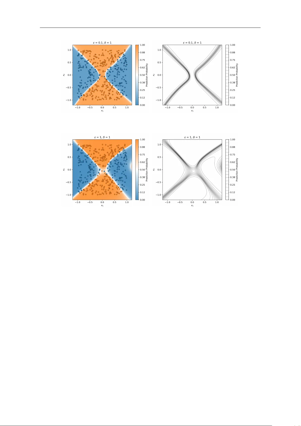
Univ ersal Appro ximation Constrain ts of Narro w ResNets: The T unnel Eﬀect Christian Kuehn 1 , 2 , 3 , Sara-Viola Kun tz 1 , 2 , 3 & T obias W¨ ohrer 4 1 T e chnic al University of Munich, Scho ol of Computation, Information and T e chnolo gy, Dep artment of Mathematics, Boltzmannstr aße 3, 85748 Gar ching, Germany 2 Munich Data Scienc e Institute (MDSI), Gar ching, Germany 3 Munich Center for Machine L earning (MCML), M¨ unchen, Germany 4 TU Wien, Dep artment of Mathematics, Institute of Analysis and Scientiﬁc Computing, Vienna, Austria Marc h 30, 2026 Abstract W e analyze the univ ersal approximation constraints of narro w Residual Neural Net works (ResNets) b oth theoretically and numerically . F or deep neural net works without input space augmen tation, a central constraint is the inability to represen t critical p oin ts of the input-output map. W e prov e that this has global consequences for target function approximations and show that the manifestation of this defect is typically a shift of the critical point to inﬁnity , whic h w e call the “tunnel eﬀect” in the con text of classiﬁcation tasks. While ResNets oﬀer greater expressivit y than standard multila yer p erceptrons (MLPs), their capability strongly dep ends on the signal ratio b et ween the skip and residual c hannels. W e establish quantitativ e approximation b ounds for b oth the residual-dominant (close to MLP) and skip-dominant (close to neural ODE) regimes. These estimates dep end explicitly on the c hannel ratio and uniform netw ork w eight b ounds. Lo w-dimensional examples further provide a detailed analysis of the diﬀeren t ResNet regimes and how architecture-target incompatibility inﬂuences the approximation error. Keyw ords: neural ODEs, deep learning, universal approximation, ResNets MSC2020: 41A30, 58K05, 68T07 .  ckuehn@ma.tum.de (Christian Kuehn)  saraviola.kun tz@ma.tum.de (Sara-Viola Kuntz)  tobias.woehrer@tuwien.ac.at (T obias W¨ ohrer) 1 Univ ersal Approximation Constrain ts of Narro w ResNets: The T unnel Eﬀect Con ten ts 1 In tro duction 3 2 Critical P oints in Residual Neural Netw orks 5 2.1 Univ ersal Approximation and Critical P oin ts . . . . . . . . . . . . . . . . . . . . . . . 5 2.2 Residual Neural Netw orks . . . . . . . . . . . . . . . . . . . . . . . . . . . . . . . . . . 6 2.3 Assumptions on Non-Augmented Arc hitectures . . . . . . . . . . . . . . . . . . . . . . 8 2.4 Existence of Critical Poin ts . . . . . . . . . . . . . . . . . . . . . . . . . . . . . . . . . 10 2.5 Global T op ological Restrictions . . . . . . . . . . . . . . . . . . . . . . . . . . . . . . . 12 2.5.1 T op ological Restrictions of Maps Without Critical Poin ts . . . . . . . . . . . . 12 2.5.2 Extension to Netw orks in Close Proximit y . . . . . . . . . . . . . . . . . . . . . 14 3 Case 0 < α ≪ 1 : Close to Neural ODEs 17 3.1 Neural ODEs . . . . . . . . . . . . . . . . . . . . . . . . . . . . . . . . . . . . . . . . . 17 3.2 Relationship to ResNets . . . . . . . . . . . . . . . . . . . . . . . . . . . . . . . . . . . 18 3.3 Existence of Critical Poin ts . . . . . . . . . . . . . . . . . . . . . . . . . . . . . . . . . 20 4 Case α ≫ 1 : Close to F eed-F orw ard Neural Netw orks 22 4.1 F eed-F orw ard Neural Netw orks . . . . . . . . . . . . . . . . . . . . . . . . . . . . . . . 22 4.2 Relationship to ResNets . . . . . . . . . . . . . . . . . . . . . . . . . . . . . . . . . . . 24 4.3 Existence of Critical Poin ts . . . . . . . . . . . . . . . . . . . . . . . . . . . . . . . . . 27 5 Examples 29 5.1 One-Dimensional ResNets . . . . . . . . . . . . . . . . . . . . . . . . . . . . . . . . . . 29 5.1.1 One-La y er ResNets . . . . . . . . . . . . . . . . . . . . . . . . . . . . . . . . . . 29 5.1.2 Multi-La y er ResNets . . . . . . . . . . . . . . . . . . . . . . . . . . . . . . . . . 32 5.1.3 Implemen tation of Two-La yer ResNets . . . . . . . . . . . . . . . . . . . . . . . 33 5.2 Tw o-Dimensional ResNets . . . . . . . . . . . . . . . . . . . . . . . . . . . . . . . . . . 35 5.2.1 Details on the Implementations . . . . . . . . . . . . . . . . . . . . . . . . . . . 36 5.2.2 Discussion of Numerical Examples . . . . . . . . . . . . . . . . . . . . . . . . . 36 6 Conclusion 39 References 40 A Relationship b et ween ResNets, Neural ODEs and FNNs 42 B Distance b et w een ResNets, Neural ODEs and FNNs 43 2 Univ ersal Approximation Constrain ts of Narro w ResNets: The T unnel Eﬀect 1 In tro duction Univ ersal appro ximation theory of neural netw orks has initially focused on shallow netw orks of arbi- trary width [ 5 , 15 ]. Ho wev er, the success of deep neural netw orks has shifted in terest tow ard architec- tures characterized by b ounded width and signiﬁcant depth [ 25 ]. As a result, researc h in recent years fo cused on determining the expressive p o wer of these practical implementations where lay er capacit y is limited. Figure 1: The “tunnel eﬀect” in non-augmen ted MLPs. It is established that b oth feedforward neural net works and neu- ral ODEs are unable to appro ximate certain functions well for narro w arc hitectures where the natural input space is not augmen ted [ 6 , 20 ]. Mathematically , a cen tral issue is the inabilit y of these mo dels’ input- output maps to express critical (or stationary) p oin ts. This topologi- cal constraint does not just hav e lo cal consequences but limits global appro ximation and generalization capabilities. The classiﬁcation of the tw o-dimensional circle to y dataset illustrates this limitation: a trained MLP with tw o neurons per la yer and an arbitrary num b er of la y ers generates a “tunnel” in the prediction level sets which leads to una v oidable misclassiﬁcations, see Figure 1 . Since the model struc- ture cannot express a critical p oin t, it m ust shift the critical p oin t to inﬁnit y whic h creates the barrier. Remark ably , the same observ a- tion holds for the structurally v ery diﬀeren t neural ODEs, where the input-output map is realized through contin uous tra jectories [ 4 , 6 ]. The structure of Residual Neural Net works (ResNets) [ 12 ] can b e understo od as “in-b et ween” classical feedforward neural netw orks (suc h as MLPs) and neural ODEs, and is able to resolve these topological constrain ts [ 22 ]. The idea of ResNets is to split eac h la yer into an iden tity c hannel that simply adv ances the lay er input unchanged and a residual c hannel that is a nonlinear transformation containing the trainable parameters. The la y er up date is form ulated as h l = h l − 1 + f ( h l − 1 , θ l ), such that the netw ork learns the diﬀerence b etw een the lay er input and the la yer output rather than the full transformation. This approach enables the training of v ery deep architectures as it provides stable gradien t computations [ 9 , 35 ]. Bey ond these remark able optimization b eneﬁts, it is striking that the arc hitecture also improv es the expressivity of the input- output map and is able to em b ed critical p oin ts without additional input augmen tation. Ho w ever, w e observe that this abilit y depends rather strongly on the c hoice of parameter initialization. Let us again consider the circle toy dataset. T raining a ResNet of width t wo, mo derate depth, and standard w eight initialization for sigmoidal activ ations, the “tunnel eﬀect” of Figure 1 t ypically does not app ear. By contrast, when the parameters are rescaled closer to 0 at initialization, the “tunnel” app ears after training. This work prov es that the “tunnel eﬀect” app ears whenever ResNets are unable to em b ed critical p oin ts but try to approximate target functions that contain suc h p oin ts. It further pro vides explicit estimates on the embedding restrictions of ResNets in the mo del parameter regimes close to MLPs and neural ODEs. This implies that ResNets that roughly maintain a balance b et ween the identit y c hannel and the transformation c hannel hav e adv an tageous expressivity in practical settings. W e form ulate these results by parameterizing the ratio b et ween the iden tity and residual channel of eac h ResNet lay er. ResNet Em b edding Capabilities Dep ending on Channel Ratio Let us outline the embedding results in more detail by assuming ResNets of constan t input width and net w ork parameters θ (w eights and biases) that are restricted to a ﬁxed parameter regime, θ ∈ Θ, where Θ fulﬁlls explicit (and reasonable in implemen tations) upper and lo wer b ounds. In this con text, w e reform ulate the ResNet la y er iteration with a skip p ar ameter ε > 0 and a r esidual p ar ameter δ > 0 as h l = εh l − 1 + δf l ( h l − 1 , θ l ) , l ∈ { 1 , . . . , L } , (1.1) where the canonical choice of the residual function is given b y f l ( θ l , h ) = f W l σ ( W l h + b l ) + ˜ b l , (1.2) 3 Univ ersal Approximation Constrain ts of Narro w ResNets: The T unnel Eﬀect 0 1 K f 1 k f α MLP regime neural ODE regime no critical p oin ts no critical p oin ts Figure 2: Expressivity of the non-augmented ResNets dep ending on the ratio α : = δ ε and the upp er and low er Lipsc hitz constan ts of the residual function. with weigh t matrices W l , f W l , bias vectors ˜ b l , b l and a sigmoidal activ ation function σ . Our goal is to sho w how the ResNets’ abilit y to express critical p oin ts dep ends on the ratio α := δ ε > 0. Let us start with p oin ting out that we can alw a ys normalize ( 1.1 ) to α = 1 b y choosing f W l = ˆ W l ε/δ . But then, w e naturally also hav e to rescale the considered mo del parameter regime Θ when comparing em b edding capabilities. Here w e take the p ersp ectiv e of ﬁxing Θ and analyzing the ex- pressivit y for diﬀerent regimes of α > 0. • 0 < α ≪ 1: In the case that α is suﬃciently small, in relation to the Lipschitz constant K f of the residual transformation f l , we sho w that ResNets are unable to express critical p oin ts. This is true indep enden tly of the n umber of ResNet la yers L . W e also show that this sp eciﬁcally holds for ResNets that are Euler discretizations of contin uous neural ODEs (where ε = 1), as long as the step size α = 1 /L is suﬃcien tly small, whic h implies that the num b er of la yers L is suﬃcien tly large. This links the discrete ResNet expressivit y to that of con tinuous neural ODEs and we pro vide explicit estimates dep ending on α and the Θ-b ounds, see Figure 2 . • α ≫ 1: In the case that the ratio α is suﬃciently large in relation to the low er Lipsc hitz constan t k f , we sho w that the ability of ResNets to express critical p oin ts also breaks down. When setting ε = 0 in ( 1.1 ), the skip connection v anishes and we recov er a standard MLP . F or such MLPs without input space augmentation, it is known that critical p oin ts cannot be em b edded, see Figure 2 . W e extend these results to ResNets with α suﬃciently large and give explicit b ounds dependent on the upp er and low er b ounds of the parameter space Θ. F or canonical residual functions ( 1.2 ) with sigmoidal activ ation functions the constan t K f is deter- mined by a uniform upp er b ound on the w eights and biases, while k f additionally relies on a uniform lo w er b ound on the singular v alues of the matrix pro duct f W l W l . W e reiterate that the expressiv- it y results remain relev an t for “standard” ResNets, where ε = δ = 1. In this case, the restrictions are expressed through the b ounds of the parameter regime Θ, necessary to obtain suitable Lipschitz constan ts K f and k f . Our theoretical results do not fo cus on the trainability of ResNet through gradien t-based al- gorithms, but rather on the fundamen tal limitations on expressivit y dep ending on the parameter regimes. T ec hniques suc h as batch normalization are training-oriented mo diﬁcations that employ related ideas. Their ob jective, how ever, is to ensure the reac hability of optimal parameters assum- ing a w ell-p osed setting. ResNets with rescaled c hannels were originally also inv estigated from such a trainability persp ectiv e [ 12 ]. T o link the implications of our theoretical results to the parameter training of ResNet mo dels, we pro vide numerical examples for the diﬀerent parameter regimes. Related W ork The work [ 22 ] pro ves universal approximation for ResNets with one-neuron hidden lay er and ReLU activ ation. According to our deﬁnitions b elo w, this corresp onds to a non-augmented ResNet arc hi- tecture of input width and hence is in agreement with our results. While the approximation sc heme is constructive, the model depth and model parameters do not represent typically trained ResNets. In comparison, we assume b ounded and smo oth activ ation functions, and pro ve weigh t dependent estimates. [ 26 ] prov es that if the weigh ts of a ResNet are initialized from a (Lipschitz) contin uous train- ing parameter function, then the parameters main tain this prop ert y throughout a gradien t descent optimization, provided the weigh ts maintain a uniform upp er b ound through rescaling (weigh t clip- ping). Our results c haracterize the expressivity of diﬀerent parameter regimes of ResNets whic h 4 Univ ersal Approximation Constrain ts of Narro w ResNets: The T unnel Eﬀect impro v es interpretabilit y . While we observe the parameter regimes remain throughout training, the corresp onding implicit regularization pro ofs are an op en problem. In [ 11 ] the expressivity of ReLU ResNets is inv estigated. The pap er c onsiders ResNets simpliﬁed to a linear structure and sho ws that if the sp ectral norm of each A l is small, x 7→ Ax cannot express non-degenerate critical p oin ts. W e prov e results of similar kind for general nonlinear ResNets. The w orks [ 25 , 37 ] in vestigate the expressivit y of ResNets but alw a ys assume augmented input spaces. Structure of the Paper In Section 2 , we introduce the considered ResNet architectures, derive their input gradien ts, and examine the global top ological restrictions caused by the absence of critical p oints. In Section 3 , we link ResNets with small channel ratios to con tinuous neural ODEs, establishing explicit approximation errors and pro ving they share the same inabilit y to em b ed critical p oin ts. In Section 4 , w e analyze large channel ratios, sho wing that ResNets behav e lik e p erturb ed feed-forward neural netw orks and similarly fail to express critical points. Finally , in Section 5 , w e present numerical exp erimen ts on lo w-dimensional datasets to illustrate the theoretical constraints and visualize the resulting “tunnel eﬀect”. 2 Critical P oin ts in Residual Neural Netw orks W e begin in Section 2.1 to recall the univ ersal approximation and univ ersal em b edding prop erties of contin uous input–output mappings relev ant to our setting. W e show that, for suc h mappings, the inability to represent a critical p oin t in a single output co ordinate implies that the univ ersal appro ximation prop ert y cannot hold. Section 2.2 introduces the Residual Neural Net work (ResNet) architectures considered in this w ork, whose lay ers dep end on a skip parameter ε and a residual parameter δ . Dep ending on the input and hidden dimensions, w e distinguish b et ween non-augmen ted and augmented arc hitectures. Section 2.3 states the sp eciﬁc assumptions on ResNets that are necessary for our analysis in the remaining part of this w ork. In Section 2.4 , w e deriv e the ResNet input gradient. In the non-augmen ted case, w e identify conditions under whic h the gradient never v anishes. In particular, we prov e that if the ratio α : = δ ε is suﬃciently small or suﬃcien tly large, the netw ork admits no critical p oin ts. Finally , Section 2.5 examines the top ological consequences of the absence of critical p oints. F or small α , the net w orks can be in terpreted as discretizations of neural ODEs, whereas for large α , they act as p erturbations of classical feed-forward neural netw orks (FNNs). In b oth regimes, we deriv e bounds on the distance to the resp ectiv e limiting mo dels and discuss the resulting top ological restrictions. 2.1 Univ ersal Appro ximation and Critical Poin ts Our goal in this w ork is to study the expressivity of ResNets dep ending on the sp eciﬁc architec- tural c hoices. F or that purpose, we specialize the general deﬁnitions of univ ersal approximation and universal embedding from [ 21 ] to the Euclidean setting, focusing on the space C k ( X , R n out ), X ⊂ R n in op en, of k -times contin uously diﬀerentiable functions f : X → R n out . W e use the max-norm ∥ y ∥ ∞ : = max i ∈{ 1 ,...,n } | y i | for vectors y ∈ R n and denote the induced sup-norm of f ∈ C k ( X , R n out ) on a set D ⊂ X b y ∥ f ∥ ∞ , D : = sup x ∈D ∥ f ( x ) ∥ ∞ = sup x ∈D max i ∈{ 1 ,...,n out } | f i ( x ) | . Deﬁnition 2.1 (Univ ersal Appro ximation [ 21 ]) . A neural netw ork family N = { Φ θ : X → R n out } θ ∈ Θ with X ⊂ R n in op en and parameters θ ∈ Θ ⊂ R p has the universal approximation prop ert y with resp ect to the space  C k ( X , R n out ) , ∥·∥ ∞ , X  , k ≥ 0, if for every ε > 0, ev ery compact subset K ⊂ X and every function Ψ ∈ C k ( X , R n out ), there exists θ ∈ Θ, suc h that ∥ Φ θ − Ψ ∥ ∞ , K < ε . 5 Univ ersal Approximation Constrain ts of Narro w ResNets: The T unnel Eﬀect As we study in the upcoming sections the input-output map of diﬀeren t neural netw ork arc hi- tectures directly , it is useful to additionally in tro duce the stronger concept of universal embedding, whic h requires an exact represen tation of the target function. Deﬁnition 2.2 (Univ ersal Embedding [ 21 ]) . A neural netw ork family N = { Φ θ : X → R n out } θ ∈ Θ with X ⊂ R n in op en and parameters θ ∈ Θ ⊂ R p has the universal em b edding prop ert y with resp ect to the space C k ( X , R n out ), k ≥ 0, if for every function Ψ ∈ C k ( X , R n out ), there exists θ ∈ Θ, such that Φ θ ( x ) = Ψ( x ) for all x ∈ X . An imp ortan t prop ert y characterizing the dynamics of the input-output map of neural net w orks Φ ∈ C 1 ( X , R n out ) with input space X ⊂ R n in op en and output space R n out , is the existence of critical p oin ts, i.e., zeros of the netw ork input gradient ∇ x Φ. It is crucial not to confuse the input gradient ∇ x Φ with the parameter gradien t ∇ θ Φ, where θ ∈ Θ denotes all parameters of the considered neural net w ork. The parameter gradien t ∇ θ Φ is needed for bac kpropagation algorithms in the training pro cess of neural net w orks. It is instructiv e to study the existence of critical points in the input-output map of diﬀerent neural netw ork arc hitectures, as this has direct implications for their embedding and approximation capabilities [ 21 ]. The following theorem implies that neural net work architectures in which at least one comp onen t map has no critical p oin t cannot hav e the univ ersal approximation property . Theorem 2.3 (Maps without Critical Poin ts are not Universal Approximators) . Consider a set of functions S ⊂ C 1 ( X , R n out ) , X ⊂ R n in op en, wher ein for every map Φ ∈ S , ther e exists a c omp onent i ∈ { 1 , . . . , n out } , such that ∇ x Φ i ( x )  = 0 for al l x ∈ X . Then the set S c annot have the universal appr oximation pr op erty with r esp e ct to the sp ac e  C k ( X , R n out ) , ∥·∥ ∞ , X  for every k ≥ 0 . Pr o of. The statement follows directly by generalizing [ 21 , Theorem 2.6] from scalar maps to m ultiple output comp onents: b y the resp ectiv e theorem, there exists a compact set K ⊂ X with non-empt y in terior int( K ), suc h that the sup-norm b et ween the quadratic function Ψ z : K → R , Ψ z ( x ) = n in X j =1 ( x j − z j ) 2 with z ∈ int( K ) (2.1) and any scalar map without any critical point cannot b e made arbitrarily small. Consequently , the quadratic function Ψ z also cannot be appro ximated with arbitrary precision b y an y of the considered comp onen t maps Φ i ∈ C 1 ( X , R ) satisfying ∇ x Φ i ( x )  = 0 for all x ∈ X , i.e., ∥ Φ i − Ψ z ∥ ∞ , K ≥ µ for some µ > 0. Hence, ev ery map Ψ ∈ C k ( X , R n out ) with i -th comp onen t map Ψ i | K = Ψ z as deﬁned in ( 2.1 ) cannot b e approximated with arbitrary precision b y any map Φ ∈ S on K , where the i -th comp onen t fulﬁlls the giv en assumptions. As Theorem 2.3 considers maps in which single output comp onen ts cannot ha v e any critical points, w e can, without loss of generalit y , restrict our up coming analysis to scalar neural netw ork architectures with n out = 1. In the recen t w ork [ 21 ], the expressivity of multila yer p erceptrons (MLPs) and neural ODEs is studied by c haracterizing the existence and regularity of critical points. One of the main results sho ws that non-augmen ted MLPs and non-augmen ted neural ODEs cannot ha ve critical p oin ts and hence lack the univ ersal approximation prop ert y (see also Section 3.3 and Section 4.3 ). In the augmen ted case, the universal approximation property of MLPs and neural ODEs is well established in the literature [ 6 , 14 , 15 , 18 , 29 , 38 ]. In the follo wing sec tions, we ﬁrst introduce ResNet architectures and then study their expressivit y using Theorem 2.3 . 2.2 Residual Neural Net w orks Residual neural netw orks (ResNets) are feedforward neural net w orks structured in la y ers h l ∈ R n hid , l ∈ { 1 , . . . , L } , consisting of n hid no des eac h. Given an initial lay er h 0 ∈ R n hid , the hidden lay ers are iterativ ely up dated b y h l = εh l − 1 + δ f l ( h l − 1 , θ l ) , l ∈ { 1 , . . . , L } , (2.2) with a (typically nonlinear) r esidual function f l : R n hid × R p l → R n hid and hidden p ar ameters θ l ∈ Θ l ⊂ R p l , where Θ l denotes the set of parameters of la yer l and Θ = Θ 1 × . . . × Θ L ⊂ R p the total 6 Univ ersal Approximation Constrain ts of Narro w ResNets: The T unnel Eﬀect parameter space of the ResNet. The la yer up date rule ( 2.2 ) includes tw o terms: a skip connection scaled by the skip p ar ameter ε > 0, and a residual term weigh ted by the r esidual p ar ameter δ > 0. In contrast to classical feed-forward neural netw orks, corresponding to the case ε = 0 and δ > 0 in ( 2.2 ) (cf. Section 4 ), the ResNet up date rule contains the linear term εh l − 1 . It is called a skip- or shortcut connection (cf. [ 12 ]), as it allows the lay er input to bypass the transformation of the residual function, see Figure 3(a) for a visualization. The residual function f l can b e an arbitrary map, but t ypical choices include f l ( h l − 1 , θ l ) : = f W l σ l ( W l h l − 1 + b l ) + ˜ b l = f W l σ l ( a l ) + ˜ b l (2.3) for l ∈ { 1 , . . . , L } with parameters θ l : = ( W l , f W l , b l , ˜ b l ) consisting of weigh t matrices W l ∈ R m l × n hid , f W l ∈ R n hid × m l , and biases b l ∈ R m l , ˜ b l ∈ R n hid . The map σ l : R → R is called an activation function , applied comp onen t-wise to the pr e-activate d states a l : = W l h l − 1 + b l ∈ R m l , as visualized in Figure 3(b) . By a sligh t abuse of notation, w e also write σ l for the component-wise extension σ l : R m l → R m l as in ( 2.3 ). The in tended meaning will b e clear from the argument. Typical choices for the activ ation function σ l include tanh, sigmoid( y ) = (1 + e − y ) − 1 or ReLU( y ) = max { 0 , y } . The hidden dimension n hid is constan t across the lay ers of the ResNet, whereas the dimension m l of the pre-activ ated state a l , which also con trols the num b er of parameters used in lay er h l , can v ary . T o b e ﬂexible in the input and output dimensions of ResNets, tw o additional transformations are applied b efore the la y er h 0 and after the lay er h L , resulting in the input-output map Φ : X → R n out , X ⊂ R n in , Φ( x ) = ˜ λ ( h L ( λ ( x ))) , (2.4) with input tr ansformation λ : R n in → R n hid , output tr ansformation ˜ λ : R n hid → R n out and comp osite map h L : R n hid → R n hid , which maps the tr ansforme d input h 0 = λ ( x ) to the last hidden la yer h L via the iterativ e up date rule ( 2.2 ). F or the ResNet architecture ( 2.4 ), we call x ∈ X the input , h 0 = λ ( x ) the tr ansforme d input , h 1 , . . . , h L the hidden layers , and Φ( x ) the output of the neural net w ork. Often, the transformations λ and ˜ λ are chosen to be aﬃne linear, but nonlinear functions are also p ossible. F or example, for classiﬁcation tasks with n out = 1, the output is often normalized to a probability , i.e., Φ( x ) ∈ [0 , 1]. h l − 1 f l ( h l − 1 , θ l ) h l · δ · ε (a) General ResNet update rule ( 2.2 ). h l − 1 a l σ l ( a l ) h l · δ · ε aﬀ. lin. aﬀ. lin. (b) ResNet update rule ( 2.3 ) with tw o aﬃne linear maps. Figure 3: Structure of the update rule of a residual neural net work with skip parameter ε and residual parameter δ . Ev ery la yer h l ∈ R n hid is represented by a square. The case ε = δ = 1 in the up date rule ( 2.2 ) corresp onds to classical ResNet arc hitectures as in tro duced in [ 12 ]. The general case with ε, δ > 0 can also b e seen as a sp ecial case of highw a y net w orks with carry gate ε and transform gate δ [ 34 ]. In the case ε = 1 and δ → 0, ResNets are connected to neural ODEs, which w e introduce in Section 3 . The case δ > 0 and ε = 0 with residual function f l as deﬁned in ( 2.3 ) leads to classical feed-forw ard neural net works, such as m ultila y er p erceptrons, introduced in Section 4 . In our up coming analysis, we fo cus on ResNets with ε, δ > 0, whic h include b oth a linear skip connection and a non-linear residual term. In the follo wing, we deﬁne the class of considered ResNet architectures. Deﬁnition 2.4 (Residual Neural Netw ork) . F or k ≥ 0, the set RN k ε,δ ( X , R n out ) ⊂ C k ( X , R n out ) with X ⊂ R n in op en, ε, δ > 0, denotes all ResNet architectures Φ : X → R n out as deﬁned in ( 2.4 ) with • input transformation λ ∈ C k ( R n in , R n hid ), • output transformation ˜ λ ∈ C k ( R n hid , R n out ), • for l ∈ { 1 , . . . , L } : residual functions f l ( · , θ l ) ∈ C k ( R n hid , R n hid ) for each ﬁxed θ l ∈ Θ l ⊂ R p l . 7 Univ ersal Approximation Constrain ts of Narro w ResNets: The T unnel Eﬀect In the case of f l of the form ( 2.3 ), the condition f l ( · , θ l ) ∈ C k ( R n hid , R n hid ) is equiv alen t to σ l ∈ C k ( R , R ) for l ∈ { 1 , . . . , L } . W e call the corresp onding ResNets c anonic al and denote the subset of c anonic al R esNet ar chite ctur es b y RN k ε,δ,σ ( X , R n out ) ⊂ RN k ε,δ ( X , R n out ) ⊂ C k ( X , R n out ). The regularit y of ResNets Φ ∈ RN k ε,δ ( X , R n out ), k ≥ 0, X ⊂ R n in op en, follows directly from the regularit y of the residual functions f l or the activ ation functions σ l , resp ectiv ely . Remark 2.5. Throughout this work, we assume strictly p ositiv e parameters ε and δ to simplify the notation. This c hoice is based on t ypical ResNets (where ε = δ = 1) and their in terpretation as neural ODE discretizations (where ε = 1, δ > 0). As most of the up coming results only dep end on the magnitude of the ratio α : = δ ε , they also extend to the case α < 0, b y considering the absolute v alue | α | in the resp ectiv e b ounds. Dep ending on the input dimension n in and the hidden dimension n hid , w e distinguish b et ween non-augmen ted and augmented ResNet arc hitectures. Deﬁnition 2.6 (ResNet Classiﬁcation) . The class of ResNets RN k ε,δ ( X , R n out ), k ≥ 0, X ⊂ R n in op en, is subdivided as follows: • Non-augmente d R esNet Φ ∈ RN k ε,δ, N ( X , R n out ): it holds n in ≥ n hid . • A ugmente d R esNet Φ ∈ RN k ε,δ, A ( X , R n out ): it holds n in < n hid . F or canonical ResNets Φ ∈ RN k ε,δ,σ ( X , R n out ), w e analogously denote non-augmen ted arc hitectures b y RN k ε,δ,σ , N ( X , R n out ) and augmented arc hitectures b y RN k ε,δ,σ , A ( X , R n out ). The concept of non-augmen ted and augmented ResNets is visualized in Figure 4 . The classiﬁcation of ResNets is indep enden t of the c hoice of the residual functions f l , and hence also indep enden t of the intermediate dimensions m l in the case of canonical ResNets. The distinction of arc hitectures b ecomes relev ant for the analysis of the expressivit y of the ResNet input-output map in the upcoming Section 2.4 and Section 2.5 . Our w ork mainly focuses on the restrictions of non-augmen ted ResNet arc hitectures induced by Theorem 2.3 . Before we calculate the ResNet input gradient in Section 2.4 to characterize the existence of critical p oin ts, we discuss in the following Section 2.3 the assumptions on non-augmented arc hitectures relev ant for our analysis. x h 0 h 1 h L Φ( x ) (a) Example of a non-augmen ted ResNet Φ ∈ RN k ε,δ, N ( R 4 , R 2 ) with n hid = 3. x h 0 h 1 h L Φ( x ) (b) Example of an augmen ted ResNet Φ ∈ RN k ε,δ, A ( R 2 , R ) with n hid = 3. Figure 4: Classiﬁcation of ResNet arc hitectures dep ending on the input and the hidden dimension. Every no de of the neural net work is represen ted as a circle. 2.3 Assumptions on Non-Augmen ted Architectures In this section, w e state the assumptions used for the analysis of non-augmented ResNet arc hitectures in Section 2.4 and Section 2.5 . These conditions also app ear in the study of ResNets related to neural ODEs (Section 3 ) and to feed-forward neural netw orks (Section 4 ). The assumptions are in tro duced b elo w for reference; each of the up coming theorems explicitly states which of the assumptions are required. 8 Univ ersal Approximation Constrain ts of Narro w ResNets: The T unnel Eﬀect Assumptions on the Activ ation F unctions Canonical ResNets Φ ∈ RN k ε,δ,σ ( X , R n out ), k ≥ 0, X ⊂ R n in op en, with residual functions as deﬁned in ( 2.3 ), depend on the component-wise applied activ ation functions σ l ∈ C k ( R , R ), l ∈ { 1 , . . . , L } . The same dep endence applies to multila yer p erceptrons, which are introduced and analyzed in Sec- tion 4 . In the following, w e state three assumptions, all of which are satisﬁed by standard sigmoidal nonlinearities suc h as tanh and sigmoid( y ) = (1 + e − y ) − 1 , but exclude activ ation functions of ReLU- t yp e. In the literature, ReLU activ ation functions are often excluded if smo othness prop erties such as the contin uity of the deriv ative is needed (cf. [ 26 ]). Assumption (A1) (Lipsc hitz Contin uous Activ ation) . The activation functions σ l ∈ C 0 ( R , R ) ar e uniformly glob al ly Lipschitz c ontinuous with Lipschitz c onstant K σ > 0 . In p articular, if σ l ∈ C 1 ( R , R ) , Lipschitz c ontinuity is e quivalent to ∥ σ ′ l ∥ ∞ , R ≤ K σ for al l l ∈ { 1 , . . . , L } . Assumption (A2) (Bounded Activ ation) . The activation functions σ l ∈ C 0 ( R , R ) ar e uniformly b ounde d, i.e., ther e exists a c onstant S > 0 such that ∥ σ l ∥ ∞ , R ≤ S for al l l ∈ { 1 , . . . , L } . Assumption (A3) (Strictly Monotone Activ ation) . The activation functions σ l ∈ C 0 ( R , R ) ar e strictly monotone for al l l ∈ { 1 , . . . , L } . In p articular, if σ l ∈ C 1 ( R , R ) , strict monotonicity is e quivalent to | σ ′ l ( y ) | > 0 for every y ∈ R and al l l ∈ { 1 , . . . , L } . Remark 2.7. The three assumptions on the activ ation functions are standard in the analytical study of deep neural netw orks. The global Lipsc hitz contin uity of Assumption (A1) ensures stability of the input-output mapping. By the mean v alue theorem, the upp er b ound of ∥ σ ′ l ∥ ∞ , R deﬁnes a Lipschitz constan t of the activ ation function. The b oundedness of the activ ation function in Assumption (A2) is relev an t when es timating the distance b et ween ResNets and neural ODEs or ResNets and MLPs. The monotonicit y Assumption (A3) guarantees non-degeneracy of the la yer-wise Jacobians and is essen tial in our analysis of critical p oin ts. Assumptions on the Parameters In the following, we form ulate t wo assumptions on the parameters appearing in the considered neural net w orks. F or a parameter tuple θ = ( A 1 , . . . , A k ) consisting of matrices or vectors A j ∈ R a j × b j , j ∈ { 1 , . . . , k } w e consider the standard Euclidean norm ∥·∥ 2 , the max-norm ∥·∥ ∞ and their induced matrix norms deﬁned by ∥ A j ∥ q : = sup x ∈ R b j \{ 0 } ∥ A j x ∥ q ∥ x ∥ q , q ∈ { 2 , ∞} . T o ensure that the up coming uniform parameter bound applies to each comp onen t of the tuple θ , w e deﬁne the norm of θ as the maxim um of the individual norms, i.e., ∥ θ ∥ q : = max j ∈{ 1 ,...,k } ∥ A j ∥ q . Since diﬀeren t arc hitectures inv olve diﬀerent parameters, their notation and dimensions are sp eciﬁed in the resp ectiv e theorems in which they are used. Assumption (B1) (Bounded Parameters) . F or a set of p ar ameters Θ ⊂ R p , al l p ar ameters ar e uniformly b ounde d in the max-norm or the Euclide an norm, i.e., ther e exist c onstants ω ∞ ≥ 0 or ω 2 ≥ 0 , such that it holds ∥ θ ∥ ∞ ≤ ω ∞ or ∥ θ ∥ 2 ≤ ω 2 r esp e ctively for al l θ ∈ Θ . Remark 2.8. • Since all norms on ﬁnite-dimensional spaces are equiv alent, uniform b oundedness in any norm is suﬃcient for Assumption (B1) . • F or a ﬁxed neural net work with a ﬁnite n umber of parameters θ , the uniform upp er b ound is trivially satisﬁed. • The assumption on b ounded parameters, especially w eight matrices, is standard in the analysis and implementation of deep neural net works. It helps prev ent explo ding gradien ts during train- ing and ensures reasonable global Lipschitz constants of the considered net works [ 27 , 28 , 32 ]. In practice, man y learning algorithms enforce these b ounds implicitly or explicitly through regularization techniques, suc h as w eight decay [ 8 ] or sp ectral regularization [ 36 ]. 9 Univ ersal Approximation Constrain ts of Narro w ResNets: The T unnel Eﬀect Assumption (B2) (F ull Rank W eight Matrices) . F or a set of p ar ameters Θ ⊂ R p , al l weight matric es W ∈ R a × b c ontaine d in Θ have ful l r ank, i.e., rank( W ) = min { a, b } . Remark 2.9. The full-rank assumption is generic, as b y [ 21 , Lemma 3.6], the subset of singular w eigh t matrices has Leb esgue measure zero. This assumption is esp ecially relev an t to pro ve the non-existence of critical p oin ts in certain non-augmented neural netw ork architectures. Assumptions on the Input and Output T ransformations W e mak e the follo wing assumption on the input and output transformations λ and ˜ λ of the considered non-augmen ted netw ork architectures with n in ≥ n hid . Assumption (C1) (Non-Singular Input and Output T ransformation) . The input and output tr ans- formations λ ∈ C 1 ( R n in , R n hid ) and ˜ λ ∈ C 1 ( R n hid , R n out ) with n in ≥ n hid fulﬁl l the fol lowing: • The Jac obian matrix ∂ x λ ( x ) ∈ R n hid × n in has ful l r ank n hid for every x ∈ R n in . • The Jac obian matrix ∂ y ˜ λ ( y ) ∈ R n out × n hid has ful l r ank min { n hid , n out } for every y ∈ R n hid . Remark 2.10. Assumption (C1) is satisﬁed if the input and output transformations λ and ˜ λ hav e the typical form of the residual function as in ( 2.3 ), such that λ ( x ) = f W 0 σ 0 ( W 0 x + b 0 ) + ˜ b 0 , ˜ λ ( y ) = f W L +1 σ L +1 ( W L +1 y + b L +1 ) + ˜ b L +1 , (2.5) with a comp onen t-wise applied activ ation function σ that satisﬁes Assumption (A3) and w eight matrices that fulﬁll Assumption (B2) , cf. [ 21 , Lemma C.1]. 2.4 Existence of Critical P oints T o understand the existence of critical p oin ts in ResNet arc hitectures, w e deriv e in the follo wing the input gradient of ResNets Φ ∈ RN 1 ε,δ ( X , R ), X ⊂ R n in op en. Due to Theorem 2.3 , we can without loss of generalit y restrict our analysis to single output comp onen ts, or equiv alently , scalar neural net w orks. The up coming prop osition applies to b oth non-augmen ted and augmented ResNets. Prop osition 2.11 (ResNet Input Gradient) . The input gr adient of a sc alar R esNet Φ ∈ RN 1 ε,δ ( X , R ) at x ∈ X , X ⊂ R n in op en, with iter ative up date rule ( 2.2 ) is given by ∇ x Φ( x ) = h ∂ h L ˜ λ ( h L ) · ( ε · Id n hid + δ · ∂ h L − 1 f L ( h L − 1 , θ L )) · · · · · · ( ε · Id n hid + δ · ∂ h 0 f 1 ( h 0 , θ 1 )) · ∂ x λ ( x ) i ⊤ ∈ R n in (2.6) with Jac obian matrix ∂ h l − 1 f l ( h l − 1 , θ l ) of the r esidual function f l with r esp e ct to the layer h l − 1 . F or c anonic al R esNets Φ ∈ RN 1 ε,δ,σ ( X , R ) with the explicit r esidual function in ( 2.3 ) , the Jac obian matrix ∂ h l − 1 f l ( h l − 1 , θ l ) of the R esNet input gr adient is given by ∂ h l − 1 f l ( h l − 1 , θ l ) = f W l σ ′ l ( a l ) W l ∈ R n hid × n hid , l ∈ { 1 , . . . , L } , with diagonal matrix σ ′ l ( a l ) : = diag( σ ′ l ([ a l ] 1 ) , . . . , σ ′ l ([ a l ] m l )) , wher e a l : = W l h l − 1 + b l ∈ R m l . Pr o of. By the multi-dimensional c hain rule applied to ResNets as deﬁned in ( 2.4 ), it holds that ∂ x Φ( x ) = ∂ Φ ∂ h L · ∂ h L ∂ h L − 1 · · · ∂ h 1 ∂ h 0 · ∂ h 0 ∂ x = ∂ h L ˜ λ ( h L ) · ( ε · Id n hid + δ · ∂ h L − 1 f L ( h L − 1 , θ L )) · · · · · · ( ε · Id n hid + δ · ∂ h 0 f 1 ( h 0 , θ 1 )) · ∂ x λ ( x ) ∈ R 1 × n in . The ﬁrst result follows b y taking the transp ose, as ∇ x Φ( x ) = [ ∂ x Φ( x )] ⊤ . 10 Univ ersal Approximation Constrain ts of Narro w ResNets: The T unnel Eﬀect F or canonical ResNets Φ ∈ RN k ε,δ,σ ( X , R ) with the explicit residual function in ( 2.3 ), the Jacobian matrix ∂ h l − 1 f l ( h l − 1 , θ l ) with resp ect to the lay er h l − 1 is given b y ∂ h l − 1 f l ( h l − 1 , θ l ) = ∂ h l − 1  f W l σ l ( W l h l − 1 + b l ) + ˜ b l  = f W l σ ′ l ( a l ) W l ∈ R n hid × n hid , for l ∈ { 1 , . . . , L } , with diagonal matrix σ ′ l ( a l ) : = diag( σ ′ l ([ a l ] 1 ) , . . . , σ ′ l ([ a l ] m l )), as the activ ation function is applied comp onen t-wise to the pre-activ ated state a l : = W l h l − 1 + b l ∈ R m l . T o apply Theorem 2.3 to residual architectures, w e form ulate the criterion for non-v anishing gradien ts via the rank of the lay er-wise Jacobians. The follo wing lemma sho ws that the rank solely dep ends on the r atio α : = δ ε of the residual parameter δ and the skip parameter ε and not on their individual size. Lemma 2.12 (La yer-Wise Jacobians) . Given l ∈ { 1 , . . . , L } , p ar ameters ε, δ > 0 , and a r esidual function f l ( · , θ l ) ∈ C 1 ( R n hid , R n hid ) with θ l ∈ Θ l ⊂ R p l , the layer-wise Jac obian at h l − 1 ∈ R n hid D l : = ε · Id n hid + δ · ∂ h l − 1 f l ( h l − 1 , θ l ) ∈ R n hid × n hid has ful l r ank if and only if − 1 α = − ε δ is not an eigenvalue of the Jac obian matrix ∂ h l − 1 f l ( h l − 1 , θ l ) . Pr o of. The statement follo ws directly from the deﬁnition of the eigenv alues of ∂ h l − 1 f l ( h l − 1 , θ l ) after rescaling the matrix D l b y 1 δ . In the case of non-augmented ResNets Φ ∈ RN 1 ε,δ, N ( X , R ), X ⊂ R n in op en, Lemma 2.12 allo ws us to form ulate conditions on the transformations λ , ˜ λ and the parameters ε and δ , under which the gradien t ∇ x Φ( x ) never v anishes for an y x ∈ X . Prop osition 2.13 (Non-Augmented ResNets without Critical Poin ts) . L et Φ ∈ RN 1 ε,δ, N ( X , R ) , X ⊂ R n in op en, ε, δ > 0 , b e a sc alar non-augmente d R esNet, which fulﬁl ls: • − 1 α = − ε δ is not an eigenvalue of the Jac obian matrix ∂ h l − 1 f l ( h l − 1 , θ l ) for al l l ∈ { 1 , . . . , L } , h l − 1 ∈ R n hid and p ar ameters θ l ∈ Θ l ⊂ R p l . • The input and output tr ansformations λ and ˜ λ fulﬁl l Assumption (C1) . Then Φ c annot have any critic al p oints, i.e., ∇ x Φ( x )  = 0 for al l x ∈ X . Pr o of. By Lemma 2.12 , all la yer-wise Jacobians D l : = ε · Id n hid + δ · ∂ h l − 1 f l ( h l − 1 , θ l ) hav e full rank for all h l − 1 ∈ R n hid and θ l ∈ Θ l . As the ResNet Φ is scalar and non-augmented, it holds n in ≥ n hid ≥ n out = 1, such that the dimensions in the matrix pro duct ( 2.6 ) are monotonically decreasing. T ogether with Assumption (C1) , it follo ws that the gradien t ∇ x Φ( x ) alw ays has full rank 1, uniformly in x ∈ X . Dep ending on the ratio α : = δ ε b et ween the skip parameter ε and the residual parameter δ , w e analyze in Section 3.3 and Section 4.3 when the ﬁrst assumption of Prop osition 2.13 is fulﬁlled. W e iden tify t w o parameter regimes, 0 < α ≪ 1 and α ≫ 1, for whic h non-augmen ted ResNets cannot ha ve an y critical p oin ts, as visualized in Figure 2 . In these parameter regimes, ResNets lac k the universal appro ximation prop ert y as implied by Theorem 2.3 . Consequently , w e extend the results of [ 21 ], regarding the non-existence of critical p oin ts in non-augmen ted neural ODEs and non-augmen ted MLPs, to ResNets. In in termediate parameter regimes of α , non-augmented ResNets can hav e the universal approxi- mation prop ert y , as demonstrated in [ 23 ] for the standard case ε = δ = 1. In contrast, for augmented ResNet arc hitectures, no equiv alent statement to Prop osition 2.13 ab out the non-existence of critical p oin ts exists. Instead, it follows analogously to [ 21 , Theorem 3.18] that due to dimension aug- men tation, critical p oin ts can exist in augmen ted arc hitectures even when all other assumptions of Prop osition 2.13 are fulﬁlled. The follo wing table pro vides an o verview of the main results of this w ork for non-augmen ted ResNets in the parameter regimes 0 < α ≪ 1 and α ≫ 1. While the previous results establish the absence of critical p oin ts in sp eciﬁc regimes, w e no w turn to a global top ological p ersp ectiv e. In the following, we quantify the expressivit y of non-augmented ResNets by measuring their distance to function classes that are already known to lac k univ ersal appro ximation. 11 Univ ersal Approximation Constrain ts of Narro w ResNets: The T unnel Eﬀect ResNets with 0 < α ≪ 1 ResNets with α ≫ 1 Regime Close to neural ODEs, as introduced in Section 3.1 Close to FNNs, suc h as MLPs, in tro- duced in Section 4.1 Distance Theorem 3.6 and Corollary 3.8 : small appro ximation error b et ween ResNets and Neural ODEs Theorem 4.12 and Corollary 4.15 : small appro ximation error b et ween ResNets and FNNs / MLPs Critical P oints Theorem 3.9 : no critical points for non- augmen ted neural ODEs Theorem 4.16 : no critical points for non- augmen ted FNNs / MLPs Theorem 3.10 : no critical points for non- augmen ted ResNets if 0 < α < 1 K f with Lipsc hitz constant K f of the residual function Theorem 4.17 : no critical p oin ts for non-augmen ted ResNets if α > 1 k f with lo w er Lipschitz constant k f of the resid- ual function T able 1: Summary of the main results regarding the relationship b etw een ResNets, neural ODEs, and FNNs, and the existence of critical points in the parameter regimes 0 < α ≪ 1 and α ≫ 1. 2.5 Global T op ological Restrictions In Section 2.4 , we discussed that non-augmented ResNets cannot hav e critical points in the parameter regimes 0 < α ≪ 1 and α ≫ 1. Complementing that direct analysis, w e c haracterize the expressivity of ResNets b y comparing them to reference netw orks Φ without critical p oin ts, such as non-augmen ted neural ODEs (cf. Theorem 3.9 ) and non-augmen ted FNNs (cf. Theorem 4.16 ). In Section 3.2 , we sho w that the distance b et ween ResNets with ε = 1 and neural ODEs scales linearly in the residual parameter δ . Similarly , in Section 4.2 , we establish that for ﬁxed δ > 0 and small ε > 0, the distance b et ween ResNets and FNNs scales asymptotically linearly in the skip parameter ε . W e divide the up coming analysis in to t w o steps. First, we establish the topological restrictions of a contin uously diﬀerentiable map Φ lac king critical p oin ts. Second, w e introduce a uniform distance b ound to sho w that these topological restrictions extend to any con tinuous neural netw ork Φ that closely approximates Φ. 2.5.1 T op ological Restrictions of Maps Without Critical Poin ts W e ﬁrst discuss the top ological implications for a reference net work Φ ∈ C 1 ( X , R ), X ⊂ R n in op en, under the assumption that ∇ x Φ( x )  = 0 for all x ∈ X . T o study how this property restricts the expressivit y of the netw ork, w e introduce level sets, sub-lev el sets, and sup er-lev el sets. Deﬁnition 2.14 (Level Sets) . Giv en f ∈ C 0 ( X , R ), X ⊂ R n in , we deﬁne the follo wing sets for c ∈ R : • Lev el set S c ( f ) : = { x ∈ X | f ( x ) = c } , • Sub-lev el set S ≤ c ( f ) : = { x ∈ X | f ( x ) ≤ c } , strict sub-level set S < c ( f ) : = { x ∈ X | f ( x ) < c } , • Super-level set S ≥ c ( f ) : = { x ∈ X | f ( x ) ≥ c } , strict sup er-lev el set S > c ( f ) : = { x ∈ X | f ( x ) > c } . The absence of critical points has direct implications on the compactness of the closed sub- and sup er-lev el sets. Although the following lemma relates to classical Morse theory , w e pro v e it directly using elementary calculus. Lemma 2.15 (Non-Compactness of Sub- and Sup er-Lev el Sets) . L et Φ ∈ C 1 ( X , R ) , ∅  = X ⊂ R n in op en, with ∇ x Φ( x )  = 0 for al l x ∈ X . Then for every c ∈ (inf x ∈X Φ( x ) , sup x ∈X Φ( x )) , the sub- and sup er-level sets S ≤ c ( Φ) and S ≥ c ( Φ) ar e non-c omp act in R n in . Pr o of. As Φ ∈ C 1 ( X , R ) has no critical p oin ts, it is non-constant around each x ∈ X , such that the in terv al (inf x ∈X Φ( x ) , sup x ∈X Φ( x )) is non-empt y . Hence, for eac h c ∈ (inf x ∈X Φ( x ) , sup x ∈X Φ( x )), 12 Univ ersal Approximation Constrain ts of Narro w ResNets: The T unnel Eﬀect the strict sub- and sup er-lev el sets S < c (Φ) and S > c (Φ) are non-empt y . Assume by contradiction that the sub-level set S ≤ c (Φ) is compact in R n in . By the extreme v alue theorem (cf. [ 31 ]), the con tin uous function Φ attains its minimum on S ≤ c (Φ) at some p oint x min . Since the strict sub- lev el set S < c (Φ) is non-empt y , there exists some y with Φ( y ) < c , which implies the minimum m ust satisfy Φ( x min ) ≤ Φ( y ) < c . As Φ is contin uous and X is op en, the strict sub-level set S < c (Φ) is an op en set in R n in and is contained in the interior int( S ≤ c (Φ)). Hence, the minimum is attained in the interior x min ∈ in t( S ≤ c (Φ)). A necessary condition for the existence of a lo cal minim um x min in the in terior of a domain for a con tin uously diﬀeren tiable function is that ∇ x Φ( x min ) = 0 [ 7 ]. This con tradicts the assumption ∇ x Φ( x )  = 0 for all x ∈ X , thus, S ≤ c (Φ) cannot b e compact in R n in . The statement for the super-level set S ≥ c (Φ) follows analogously by replacing the considered min- im um with the maximum x max attained in the interior in t( S ≥ c (Φ)). Lemma 2.15 has direct implications on classiﬁcation tasks, where decision b oundaries are deﬁned as lev el sets. In the following, we state the classical binary classiﬁcation problem in an abstract form (cf. [ 2 ]). Throughout this section, we consider a compact domain ∅  = K ⊂ R n in as our reference frame, since practical classiﬁcation datasets are b ounded. Deﬁnition 2.16 (Binary Classiﬁcation Problem) . F or a compact set ∅  = K ⊂ R n in and c 0 , c 1 ∈ R with c 0 < c 1 consider a given dataset A c 0 ,c 1 : = n ( x i , y i ) N data i =1 | x i ∈ K , y i ∈ { c 0 , c 1 } o . A function Φ ∈ C 0 ( K , R ) successfully classiﬁes A c 0 ,c 1 if there exists c ∗ ∈ ( c 0 , c 1 ), such that A c 0 : = n ( x i ) N data i =1 | ( x i , c 0 ) ∈ A c 0 ,c 1 o ⊂ S < c ∗ (Φ) , A c 1 : = n ( x i ) N data i =1 | ( x i , c 1 ) ∈ A c 0 ,c 1 o ⊂ S > c ∗ (Φ) . The level set S c ∗ (Φ) is called the decision b oundary of Φ. F or a giv en dataset, the goal of a classiﬁcation problem is to classify correctly as many data p oin ts as p ossible. As w e study in this section the top ological restrictions induced by neural net works without critical points independently of a speciﬁc dataset, w e fo cus on the topology of level sets, esp ecially the decision b oundary . F or a reference map Φ without critical p oin ts, the topology of its decision b oundary is strictly constrained. W e separate the one-dimensional case from the higher- dimensional case n in ≥ 2, as the b oundary of a compact set K is disconnected in one dimension but can b e connected in higher dimensions, leading to diﬀerent topological restrictions on the decision b oundary . One-Dimensional Case In the one-dimensional case n in = 1, Lemma 2.15 is equiv alen t to the fact that all one-dimensional maps without critical points are strictly monotone. Naturally , it follo ws that strictly monotone maps cannot satisfactorily appro ximate non-monotone target functions. This fact can also b e form ulated from the p erspective of binary classiﬁcations. F or a strictly increasing map Φ ∈ C 1 ( X , R ) and any c ∗ ∈ Φ( X ), there exists a unique x c ∗ ∈ X with Φ( x c ∗ ) = c ∗ , and the strict level sets tak e the form S < c ∗ (Φ) = ( −∞ , x c ∗ ) ∩ X , S c ∗ (Φ) = { x c ∗ } , S > c ∗ (Φ) = ( x c ∗ , ∞ ) ∩ X . (2.7) This implies that for such functions Φ, any dataset whose classes A c 0 and A c 1 cannot b e separated b y tw o disjoint interv als, cannot b e successfully classiﬁed. Therefore, Φ can only separate data that is split into t wo disjoin t interv als. Higher-Dimensional Case If the boundary ∂ K is connected, Lemma 2.15 has direct implications for nested datasets, suc h as the tw o-dimensional circle dataset, where one class is entirely surrounded b y another. T o perfectly classify such a dataset, the decision b oundary S c ∗ (Φ) would need to form a closed curv e (or a hypersphere for n in > 2), con tained en tirely within the in terior of the compact 13 Univ ersal Approximation Constrain ts of Narro w ResNets: The T unnel Eﬀect domain K . Ho wev er, this would create a strictly bounded, and therefore compact, sub- or sup er-lev el set S ≤ c ∗ (Φ) or S ≥ c ∗ (Φ), which directly con tradicts Lemma 2.15 . As w e show in the up coming Theorem 2.18 , this implies that any decision boundary attempting to separate a nested dataset is mathematically forced to in tersect the domain boundary ∂ K . When minimizing the empirical classiﬁcation error, the natural geometric compromise is to form a “tunnel”, a contin uous, narro w region of the inner class extending to the boundary ∂ K . As illustrated in the in tro duction in Figure 1 , this top ology eﬀectiv ely shifts the required critical point outside of the observ ation domain K . W e will visualize the higher-dimensional “tunnel eﬀect” in the following section, where we demonstrate that these topological limitations transfer to any net work Φ in close pro ximit y to Φ. 2.5.2 Extension to Net works in Close Pro ximity In the upcoming analysis, we study the top ological restrictions implied b y a small distance in the sup- norm b et ween a function Φ ∈ C 0 ( X , R ), X ⊂ R n in op en, and a second reference map Φ ∈ C 1 ( X , R ) without critical p oin ts, i.e., ∇ x Φ( x )  = 0 for all x ∈ X . W e assume that there exists µ > 0, such that on a compact set K ⊂ X it holds that   Φ − Φ   ∞ , K ≤ µ. (2.8) The reference map Φ may be a neural ODE, an MLP , or a ResNet in the restricted parameter regimes 0 < α ≪ 1 or α ≫ 1 identiﬁed in Section 2.4 . The estimate ( 2.8 ) implies that the map Φ is trapp ed in a µ -tube around Φ. As we will sho w, this forces the topological limitations of Φ discussed in Section 2.5.1 to carry ov er to Φ. Again, we treat the one-dimensional and higher-dimensional cases separately , as the b oundary ∂ K of a compact set is disconnected in one dimension, but can b e connected in higher dimensions. One-Dimensional Case While ev ery one-dimensional map Φ without critical p oin ts is strictly monotone, the µ -close map Φ is allow ed to oscillate and p ossess critical p oints. How ever, as the distance b et ween Φ and Φ is b ounded, the level sets of Φ hav e top ological restrictions, to o. Theorem 2.17 (T opological Restrictions for n in = 1) . Consider Φ ∈ C 0 ( X , R ) with X ⊂ R op en, and Φ ∈ C 1 ( X , R ) with ∇ x Φ( x )  = 0 for al l x ∈ X . L et ∅  = K = [ k 0 , k 1 ] ⊂ X b e a c omp act interval and a = Φ( k 0 ) , b = Φ( k 1 ) . If   Φ − Φ   ∞ , K ≤ µ < | b − a | 2 , then for any c ∈ (min( a, b ) + µ, max( a, b ) − µ ) , none of the sub- and sup er-level sets S < c (Φ) and S > c (Φ) c an b e entir ely c ontaine d within the interior int( K ) = ( k 0 , k 1 ) . Pr o of. Without loss of generality , we assume that Φ is strictly monotonically increasing, suc h that a < b . The b ound for the distance b et ween Φ and Φ implies that Φ( k 0 ) ≤ Φ( k 0 ) + µ = a + µ, and Φ( k 1 ) ≥ Φ( k 1 ) − µ = b − µ. Since µ < | b − a | 2 , the interv al ( a + µ, b − µ ) is non-empt y , such that for any c ∈ ( a + µ, b − µ ) it follo ws Φ( k 0 ) < c < Φ( k 1 ). Consequently , any sub-lev el set S < c (Φ) must contain k 0 and any sup er-lev el set S > c (Φ) m ust contain k 1 , suc h that the statement follo ws. By symmetry , the same argumen tation holds for monotonically decreasing maps. Theorem 2.17 implies that Φ cannot correctly classify any dataset A c 0 ,c 1 where the b oundary p oin ts k 0 , k 1 b elong to the same class but surround a diﬀeren t inner class. W e visualize these constraints in Figure 5 using a centered classiﬁcation task. The data points are subdivided in tw o classes via the quadratic function Ψ z : K = [ k 0 , k 1 ] → R , Ψ z ( x ) = ( x − z ) 2 with z ∈ ( k 0 , k 1 ) in the following wa y: all data points in the region S < c ∗ (Ψ z ) are assigned the lab el c 0 , whereas all data p oin ts in the region S > c ∗ (Ψ z ) are assigned the lab el c 1 . The function Ψ z w as also used in Theorem 2.3 to show that functions without critical p oin ts cannot hav e the universal appro ximation prop ert y . 14 Univ ersal Approximation Constrain ts of Narro w ResNets: The T unnel Eﬀect On the one hand, the map Φ can form local minima to better appro ximate the given data than the strictly monotone map Φ, as sho wn in Figure 5 . On the other hand, Φ is trapped in a µ -tube around Φ, suc h that its lev el sets S < c ∗ (Φ) and S > c ∗ (Φ) can b e disconnected, but cannot b e en tirely contained in the in terv al ( k 0 , k 1 ). Figure 5 sho ws that the classiﬁcation of Φ improv es ov er the classiﬁcation of Φ, but Theorem 2.17 guarantees failure of a p erfect classiﬁcation. R R R R z k 0 k 1 k 0 k 1 k 0 k 1 Ψ z ( x ) µ c ∗ Φ( x ) Φ( x ) Lev el Sets of Φ Lev el Sets of Φ Blue: S < c ∗ Gra y: S c ∗ Orange: S > c ∗ Figure 5: T op ological restrictions induced by the absence of critical p oin ts in the one-dimensional case: the neural netw ork Φ has limited accuracy when classifying the data deﬁned by the lev el sets of the quadratic function Ψ z , as it is trapp ed in a µ -tub e around a strictly monotonically increasing reference function Φ. Higher-Dimensional Case In the higher-dimensional case n in ≥ 2, the boundary ∂ K of a compact set K can b e connected, whic h fundamentally changes the topological restrictions compared to the one-dimensional case. The following theorem prov es that the decision b oundary S c ∗ (Φ) of a map Φ that is µ -close to a reference map Φ without critical p oin ts cannot b e entirely con tained within the in terior of K , but instead m ust intersect the boundary ∂ K . Theorem 2.18 (T op ological Restrictions for n in ≥ 2) . Consider Φ ∈ C 0 ( X , R ) with X ⊂ R n in op en, n in ≥ 2 , and Φ ∈ C 1 ( X , R ) with ∇ x Φ( x )  = 0 for al l x ∈ X . L et ∅  = K ⊂ X b e a c omp act set with a c onne cte d b oundary ∂ K , and let [ a, b ] ⊂ Φ( K ) b e a non-empty interval. If   Φ − Φ   ∞ , K ≤ µ < b − a 2 , then for al l c ∈ ( a + µ, b − µ ) , the level set S c (Φ) interse cts the b oundary ∂ K , i.e., S c (Φ) ∩ ∂ K  = ∅ . Pr o of. Let 0 < ν < b − a 2 − µ b e arbitrary . Since [ a, b ] ⊂ Φ( K ), the sub-lev el set S : = S ≤ a + ν (Φ) has a non-empt y intersection with the domain K . With the assumptions on Φ and Φ and a + ν ∈ (inf x ∈X Φ( x ) , sup x ∈X Φ( x )), it follows from Lemma 2.15 that S is non-compact in R n in . F urthermore, b y the contin uity of Φ, the set S = Φ − 1 (( −∞ , a + ν ]) is closed in X . W e ﬁrst show that S m ust in tersect the b oundary of K , as visualized in Figure 6 . Assume b y con tradiction that S ∩ ∂ K = ∅ . Since there exists x ∗ ∈ K with Φ( x ∗ ) = a , the intersection S ∩ K is non-empt y . If this intersection do es not intersect the b oundary ∂ K , then S ∩ K is entirely con tained in the interior int( K ). Because S is closed and K is compact, their intersection S ∩ K is compact, to o. The con tin uous function Φ must then attain its global minim um on the compact set S ∩ K at some p oin t x min . As S ∩ K ⊂ int( K ), x min w ould b e an interior p oin t of K . A necessary condition for the existence of the minim um x min of the con tin uously diﬀeren tiable function Φ : int( K ) → R is that ∇ x Φ( x min ) = 0, as int( K ) ⊂ R n in is an op en set [ 7 ]. This contradicts the assumption that Φ has no critical p oints, thus it follows that S ∩ ∂ K  = ∅ . By an analogous argument applied to the sup er-lev el set S ≥ b − ν (Φ), we conclude that: S ≤ a + ν (Φ) ∩ ∂ K  = ∅ and S ≥ b − ν (Φ) ∩ ∂ K  = ∅ . (2.9) 15 Univ ersal Approximation Constrain ts of Narro w ResNets: The T unnel Eﬀect S ≥ b − ν (Φ) S ≥ b − ν − µ (Φ) S c (Φ) S ≤ a + ν + µ (Φ) S := S ≤ a + ν (Φ) ∂ K Figure 6: Geometry of the level sets in the pro of of Theorem 2.18 . As the reference map Φ has no critical p oin ts, the level sets S ≤ a + ν (Φ) and S ≥ b − ν (Φ) must intersect the connected boundary ∂ K . As the distance b et ween Φ and Φ is b ounded, also the lev el sets S ≤ a + ν + µ (Φ) and S ≥ b − ν − µ (Φ) hav e to in tersect ∂ K . Any decision b oundary S c (Φ) forced in b et ween S ≤ a + ν + µ (Φ) and S ≥ b − ν − µ (Φ) has to intersect ∂ K , too. S c (Φ) S c (Φ) ∂ K Figure 7: T op ological failure on the circle dataset. The decision b oundary S c (Φ) has to intersect the b oundary ∂ K , as the reference map Φ has no criti- cal p oin ts. Even though Φ can ha ve critical p oin ts in K , the fact that Φ is µ -close to Φ means S c (Φ) m ust still intersect ∂ K . T o optimize the classiﬁ- cation under these constraints, the net work forms a “tunnel”. The uniform estimate   Φ − Φ   ∞ , K ≤ µ implies the following set inclusions: S ≤ a + ν (Φ) ⊂ S ≤ a + ν + µ (Φ) and S ≥ b − ν (Φ) ⊂ S ≥ b − ν − µ (Φ) . (2.10) Com bining the prop erties ( 2.9 ) and ( 2.10 ) yields: S ≤ a + ν + µ (Φ) ∩ ∂ K  = ∅ and S ≥ b − ν − µ (Φ) ∩ ∂ K  = ∅ . (2.11) The setting is visualized in Figure 6 . The in tersections ( 2.11 ) imply the existence of a p oin t x a ∈ ∂ K with Φ( x a ) ≤ a + ν + µ and a p oin t x b ∈ ∂ K with Φ( x b ) ≥ b − ν − µ . Since Φ is contin uous and the b oundary ∂ K is a connected subset of R n in , the image Φ( ∂ K ) is an interv al in R by the intermediate v alue prop erty [ 30 , Corollary 22.3]. Given the assumption on ν , w e ha v e a + ν + µ < b − ν − µ , which implies: [ a + ν + µ, b − ν − µ ] ⊂ [Φ( x a ) , Φ( x b )] ⊂ Φ( ∂ K ) . Since ν > 0 w as arbitrary , it follows that for every c ∈ ( a + µ, b − µ ), there exists some x c ∈ ∂ K such that Φ( x c ) = c . Therefore, the level set S c (Φ) necessarily intersects the b oundary ∂ K . Remark 2.19. The distinction b et ween the one-dimensional and higher-dimensional case lies in the top ology of the b oundary ∂ K of the compact domain K . In one dimension, the boundary of a compact in terv al consists of t w o disjoin t points and is therefore never connected. In higher dimensions ( n in ≥ 2), the b oundary of a compact set is for example connected for all conv ex sets K . In the con text of classiﬁcation problems (cf. Deﬁnition 2.16 ), Theorem 2.18 reveals a severe struc- tural limitation for nested datasets. A protot ypical example is the tw o-dimensional circle dataset (see Figure 7 ), where an inner cluster of one class is completely surrounded b y p oin ts of the other class. As discussed in Section 2.5.1 , to p erfectly classify this dataset, an ideal decision b oundary w ould need to form a closed curv e contained en tirely within the interior of the compact domain K . The classiﬁcation problem deﬁned by the circle dataset can b e generalized to any dimension n in ≥ 2 using a quadratic function Ψ z : K → R , Ψ z ( x ) = n in X j =1 ( x j − z j ) 2 with z ∈ int( K ) . 16 Univ ersal Approximation Constrain ts of Narro w ResNets: The T unnel Eﬀect F or an appropriate c ∗ ∈ R , all data p oin ts in the sub-level set S < c ∗ (Ψ z ) (an n in -dimensional ball) are assigned the lab el c 0 , while the sup er-lev el set S > c ∗ (Ψ z ) deﬁnes the class c 1 surrounding the class c 0 . Theorem 2.18 implies that suc h datasets cannot b e perfectly classiﬁed b y a map Φ that is µ -close to a reference map Φ without critical p oin ts. Because Φ lacks critical p oin ts, its decision b oundary S c ∗ (Φ) is forced to intersect the b oundary ∂ K . Since the map Φ is trapp ed in a µ -tub e around Φ, its decision b oundary S c ∗ (Φ) inherits this prop ert y and is also forced to intersect ∂ K , as visualized in Figure 7 . In con trast to Φ, the map Φ can in principle hav e critical p oints in the interior of the domain K . Nev ertheless, the map Φ cannot isolate the inner class c 0 with an n in -dimensional h yp ersphere as a decision b oundary . Instead, a natural geometric compromise o ccurs: the net work forms a “tunnel”, a contin uous, narrow region of class c 0 extending to the b oundary ∂ K . Eﬀectively , this topology shifts the required critical p oin t outside the observ ation domain K , allowing the decision b oundary S c ∗ (Φ) to reach ∂ K while still minimizing the empirical classiﬁcation error. 3 Case 0 < α ≪ 1 : Close to Neural ODEs In Section 3.1 , we in tro duce neural ordinary diﬀeren tial equations (neural ODEs). Next, we motiv ate the study of neural ODEs in Section 3.2 b y showing that neural ODEs and ResNets with suﬃcien tly small α : = δ ε can be in terpreted as discrete and contin uous coun terparts of the same underlying dynamics. Additionally , we calculate the approximation error b et ween the neural ODE and ResNet dynamics ari sing from an explicit Euler discretization. Finally , we sho w in Section 3.3 that, in analogy to non-augmented neural ODEs, critical p oin ts cannot exist in non-augmented ResNets if 0 < α ≪ 1. 3.1 Neural ODEs In this section, we in tro duce neural ODEs, whic h can b e interpreted as the inﬁnite-depth limit of ResNets. In analogy to ResNets, w e include t wo additional transformations b efore and after the initial v alue problem, and we distinguish b et ween non-augmen ted and augmen ted architectures. W e consider neural ODEs based on the solution h : [0 , T ] → R n hid of an initial v alue problem d h d t = f ( h ( t ) , θ ( t )) , h (0) = a ∈ A ⊂ R n hid , (3.1) with a non-autonomous vector ﬁeld f : R n hid × R p → R n hid , parameter function θ ∈ Θ NODE ⊂ C 0 ([0 , T ] , R p ), and a non-empt y set of p ossible initial conditions A ⊂ R n hid . When required, the solution with initial condition h (0) = a is denoted by h a ( t ) to emphasize the dependence on the initial condition. As with ResNets, we allow ﬂexibility regarding the input and output dimensions of neural ODEs. W e deﬁne neur al ODEs as the input-output maps given b y Φ : X → R n out , Φ( x ) = ˜ λ ( h λ ( x ) ( T )) , (3.2) with X ⊂ R n in op en, input transformation λ : R n in → R n hid , and output transformation ˜ λ : R n hid → R n out . T o more easily distinguish betw een neural ODE and ResNet arc hitectures, we denote them in this section as Φ and Φ, resp ectiv ely . As with ResNets, λ and ˜ λ are often chosen to b e aﬃne linear, but they can also b e nonlinear maps. The architecture ( 3.2 ) depends on the time- T map h λ ( x ) ( T ) of the initial v alue problem ( 3.1 ). W e assume that for every a ∈ A , the solution of ( 3.1 ) exists on the entire time in terv al [0 , T ]. In the up coming deﬁnition, w e denote by C i,j ( X × Y , Z ) the space of functions f : X × Y → Z that are i -times con tinuously diﬀerentiable in the ﬁrst v ariable and j -times con tin uously diﬀerentiable in the second v ariable. Deﬁnition 3.1 (Neural ODE) . F or k ≥ 1, w e denote b y NODE k ( X , R n out ) the set of all neural ODE arc hitectures Φ : X → R n out , X ⊂ R n in op en, deﬁned b y ( 3.2 ) with • input transformation λ ∈ C k ( R n in , R n hid ), • output transformation ˜ λ ∈ C k ( R n hid , R n out ), • parameter function θ ∈ Θ NODE ⊂ C 0 ([0 , T ] , R p ), 17 Univ ersal Approximation Constrain ts of Narro w ResNets: The T unnel Eﬀect • v ector ﬁeld f ∈ C k, 0 ( R n hid × R p , R n hid ) with a set of p ossible initial conditions A ⊂ R n hid , suc h that there exists a unique solution of ( 3.1 ) on [0 , T ] for every a ∈ A . The set of p ossible initial conditions of ( 3.1 ) is deﬁned by A : = λ ( X ), as the input x ∈ X ⊂ R n in of the neural ODE is mapp ed under the transformation λ to a = λ ( x ). The regularity of neural ODEs Φ ∈ NODE k ( X , R n out ) follows directly from the regularity of the v ector ﬁeld f , as explained in [ 21 , Lemma 4.3]. W e restrict Deﬁnition 3.1 to the case k ≥ 1 to guaran tee uniqueness of solution curv es of ( 3.1 ) and hence well-posedness of the neural ODEs. Remark 3.2. The regularit y assumptions on the v ector ﬁeld f and the parameter function θ can be w eak ened by considering, for example, the Carath ´ eo dory conditions (cf. [ 10 ]), as discussed in [ 20 ]. In this wa y , the parameter function θ do es not need to b e contin uous, allo wing t ypical c hoices such as piecewise constant parameter functions (cf. [ 4 ]). The follo wing classiﬁcation of non-augmen ted and augmented neural ODEs is indep enden t of the c hoice of the vector ﬁeld f and applies to all neural ODEs Φ ∈ NODE k ( X , R n out ). The concept of non-augmen ted and augmented neural ODEs is illustrated in Figure 8 . Deﬁnition 3.3 (Neural ODE Classiﬁcation) . The class of neural ODEs denoted b y NODE k ( X , R n out ), k ≥ 1, X ⊂ R n in op en, is subdivided as follows: • Non-augmente d neur al ODE Φ ∈ NODE k N ( X , R n out ): it holds n in ≥ n hid . • A ugmente d neur al ODE Φ ∈ NODE k A ( X , R n out ): it holds n in < n hid . x λ ( x ) h ( T ) Φ( x ) ODE (a) Example of a non-augmented neural ODE Φ ∈ NODE k N ( R 4 , R ) with n hid = 3. x λ ( x ) h ( T ) Φ( x ) ODE (b) Example of an augmented neural ODE Φ ∈ NODE k A ( R 3 , R 2 ) with n hid = 4. Figure 8: Classiﬁcation of neural ODE architectures depending on the dimension of the input data and the v ector ﬁeld. Figure 8(a) - (b) is adapted from [ 21 , Figure 4.1(a)-(b)]. 3.2 Relationship to ResNets The following prop osition demonstrates that, giv en our precise deﬁnitions, ResNets (cf. Deﬁnition 2.4 ) and neural ODEs (cf. Deﬁnition 3.1 ) can b e understo od as discrete and con tinuous counterparts of the same underlying dynamics. This is based on the well-established observ ation that ResNets can b e in terpreted as the explicit Euler discretization of neural ODEs [ 35 ]. Prop osition 3.4 (Relationship b et ween ResNets and Neural ODEs) . L et X ⊂ R n in b e op en, k ≥ 1 . (a) Given L ∈ N ≥ 1 and Φ ∈ NODE k ( X , R n out ) deﬁne d over [0 , T ] , the explicit Euler discr etization of Φ with step size δ : = T L r esults in a R esNet Φ ∈ RN k 1 ,δ ( X , R n out ) with L hidden layers. (b) L et Φ ∈ RN k ε,δ ( X , R n out ) b e a R esNet with L hidden layers. If the p ar ameter dimensions ar e c onstant, the layer functions ar e identic al, i.e., p l = p and f l ( · , θ l ) : = f RN ( · , θ l ) for al l l ∈ { 1 , . . . , L } , and f RN ∈ C k, 0 ( R n hid × R p , R n hid ) , then ther e exists a neur al ODE Φ ∈ NODE k ( X , R n out ) deﬁne d over [0 , Lδ ] such that Φ is its explicit Euler discr etization. The proof of this prop osition relies on standard arguments and mainly consists of translating the notation b et ween ResNets and discretized neural ODEs. It is therefore prov en in App endix A.1 and included for completeness. The following remark argues that the assumptions of Proposition 3.4(b) are not restrictive in t ypical settings. 18 Univ ersal Approximation Constrain ts of Narro w ResNets: The T unnel Eﬀect Remark 3.5. The assumption p l = p that the lay er parameters are of constant dimension for all l ∈ { 1 , . . . , L } can b e established for any given Φ ∈ RN k ε,δ ( X , R n out ) b y setting p = max { p 1 , . . . , p L } and adding zero comp onen ts to every strictly smaller p l . F urthermore, the assumption f l ( · , θ l ) : = f RN ( · , θ l ) for l ∈ { 1 , . . . , L } is fulﬁlled if the residual function f l is of the typical form ( 2.3 ) with σ l = σ for every lay er. The dep endence on the lay er l is then only enco ded in the parameters θ l ∈ Θ l ⊂ R p l . Finally , the additional assumption f RN ∈ C k, 0 ( R n hid × R p , R n hid ) in part (b) requires joint con ti- n uit y of the residual function in b oth the hidden state h and the parameters θ . This is not restrictive in practice: for canonical ResNets Φ ∈ RN k ε,δ,σ ( X , R n out ) with activ ation function σ ∈ C k ( R , R ), the residual function ( 2.3 ) is a comp osition of matrix-vector pro ducts and con tinuous nonlinearities, and hence automatically satisﬁes f RN ∈ C k, 0 ( R n hid × R p , R n hid ). In the following, we explicitly calculate the approximation error betw een the ResNet and neural ODE arc hitectures considered, thereby adapting [ 33 , Prop osition 1] to the more general neural ODE arc hitecture of Deﬁnition 3.1 . The follo wing theorem sho ws that the global error of the input-output map b et w een neural ODEs and their explicit Euler discretization dep ends linearly on the step size or residual parameter δ . Unless stated otherwise, w e alw ays consider Lipschitz constants with respect to the max-norm. Theorem 3.6 (Approximation Error b et ween ResNets and Neural ODEs) . Consider a neur al ODE Φ ∈ NODE 1 ( X , R n out ) , X ⊂ R n in op en, b ase d on the initial value pr oblem d h d t = f ( h ( t ) , θ ( t )) , h (0) = a ∈ A ⊂ R n hid , (3.3) on the time interval t ∈ [0 , T ] with the fol lowing pr op erties: • The ve ctor ﬁeld f ∈ C 1 , 1 ( R n hid × R p , R n hid ) is c ontinuously diﬀer entiable. • The set of p ossible p ar ameter functions fulﬁl ls Θ NODE ⊂ C 1 ([0 , T ] , R p ) . • The output tr ansformation ˜ λ has glob al Lipschitz c onstant K ˜ λ . • The ve ctor ﬁeld f has glob al Lipschitz c onstant K θ with r esp e ct to the ﬁrst variable h , and the solution h : [0 , T ] → R n hid has a b ounde d se c ond derivative M θ : = sup t ∈ [0 ,T ] ∥ h ′′ ( t ) ∥ ∞ uniformly for al l θ ∈ Θ NODE . Fix L ∈ N ≥ 1 , then the R esNet Φ ∈ RN 1 1 ,δ ( X , R n out ) obtaine d by Euler’s explicit metho d with step size δ : = T L and the same tr ansformations λ , ˜ λ , has the iter ative up date rule h l = h l − 1 + δ · f ( h l − 1 , θ l ) , θ l : = θ (( l − 1) δ ) , l ∈ { 1 , . . . , L } , with h 0 = h (0) . The glob al appr oximation err or b etwe en the neur al ODE and the c orr esp onding R esNet is b ounde d by   Φ − Φ   ∞ , X ≤ K ˜ λ · M θ δ 2 K θ ·  e K θ T − 1  . (3.4) Pr o of. By the regularit y assumptions f ∈ C 1 , 1 ( R n hid × R p , R n hid ) and θ ∈ Θ NODE ⊂ C 1 ([0 , T ] , R p ), the solution h : [0 , T ] → R n hid is twice contin uously diﬀerentiable. As Φ and Φ are based on the same input transformation λ , it holds h 0 = h (0) for every input x ∈ X . According to [ 1 , Theorem 6.3], the error b et w een the solution of ( 3.3 ) and the discrete solution { h 0 , . . . , h L } obtained b y Euler’s explicit metho d satisﬁes max l ∈{ 0 ,...,L } ∥ h ( t l ) − h l ∥ ∞ ≤ M θ δ 2 K θ ·  e K θ T − 1  with constants K θ , M θ and step size δ = T L , uniformly in x ∈ X . Consequently , it follo ws for the appro ximation error b et ween the ResNet and the neural ODE that   Φ − Φ   ∞ , X = sup x ∈X   ˜ λ ( h L ) − ˜ λ ( h ( T ))   ∞ ≤ K ˜ λ · M θ δ 2 K θ · max l ∈{ 0 ,...,L } ∥ h ( t l ) − h l ∥ ∞ using the Lipschitz con tinuit y of the output transformation ˜ λ . This completes the pro of. 19 Univ ersal Approximation Constrain ts of Narro w ResNets: The T unnel Eﬀect Remark 3.7. While w e fo cus on the explicit Euler discretization due to its direct structural relation to standard ResNets, higher-order n umerical sc hemes suc h as Runge-Kutta metho ds can b e used to obtain tigh ter error b ounds. In the discrete setting, these higher-order methods corresp ond to m ulti-step ResNet architectures [ 9 , 24 ]. W e now sp ecialize Theorem 3.6 to canonical ResNets with the t ypical residual function ( 2.3 ). The pro of consists of explicitly computing the constants M θ and K θ and is given in App endix B.1 . Corollary 3.8 (Appro ximation Error betw een canonical ResNets and Neural ODEs) . Consider a neur al ODE Φ ∈ NODE 1 ( X , R n out ) , X ⊂ R n in op en, b ase d on the initial value pr oblem d h d t = f W σ ( W h ( t ) + b ) + ˜ b, h (0) = h 0 ∈ R n hid , with p ar ameters ( W , f W , b, ˜ b ) ∈ Θ ⊂ R m × n hid × R n hid × m × R m × R n hid on the time interval t ∈ [0 , T ] with the fol lowing pr op erties: • The activation function σ ∈ C 1 ( R , R ) fulﬁl ls Assumptions (A1) and (A2) , i.e., ther e exist c onstants S σ , K σ > 0 with ∥ σ ∥ ∞ , R ≤ S σ and ∥ σ ′ ∥ ∞ , R ≤ K σ . • The output tr ansformation ˜ λ has glob al Lipschitz c onstant K ˜ λ . • The weight matric es W , f W , and the biases ˜ b fulﬁl l Assumption (B1) with r esp e ct to the max- norm, i.e., ther e exist c onstants ω ∞ , e ω ∞ , ˜ β ∞ ≥ 0 , such that ∥ W ∥ ∞ ≤ ω ∞ ,   f W   ∞ ≤ e ω ∞ and   ˜ b   ∞ ≤ ˜ β ∞ for al l ( W, f W , b, ˜ b ) ∈ Θ . Then, with the notation fr om The or em 3.6 it fol lows that   Φ − Φ   ∞ , X ≤ K ˜ λ ·  e ω ∞ S σ + ˜ β ∞  · δ 2 ω ∞ ·  e K σ e ω ∞ ω ∞ T − 1  . (3.5) The preceding theorem and corollary show that, in the limit δ → 0, neural ODEs and the cor- resp onding ResNets can b e view ed as con tin uous and discrete realizations of the same underlying dynamics. In the setting of Theorem 3.6 , this corresp ondence holds for ResNets with skip parameter ε = 1. More generally , ResNets with arbitrary skip parameter ε  = 1 are also related to neural ODEs, as discussed in Prop osition 3.4(b) . In this general case, taking the limit δ → 0 for ﬁxed ε > 0 means α : = δ ε → 0, as also discussed in Sections 2.4 and 2.5 . 3.3 Existence of Critical P oints In this section, w e characterize the existence of critical p oin ts in neural ODEs and ResNets in the parameter regime 0 < α ≪ 1. F or that purpose, w e ﬁrst extend the result of [ 21 ] that non-augmented neural ODEs cannot ha v e any critical p oin ts to our setting of general input and output transforma- tions. Theorem 3.9 (No Critical Poin ts in Non-Augmented Neural ODEs) . L et Φ ∈ NODE 1 N ( X , R ) , X ⊂ R n in op en, b e a sc alar non-augmente d neur al ODE and let the input and output tr ansformations λ , ˜ λ fulﬁl l Assumption (C1) . Then Φ c annot have any critic al p oints, i.e., ∇ x Φ( x )  = 0 for al l x ∈ X . Pr o of. As Φ ∈ C 1 ( X , R ), we can calculate the netw ork input gradient with the m ulti-dimensional c hain rule, which yields ∇ x Φ( x ) = ( ∂ x λ ( x )) ⊤ ( ∂ a h a ( T )) ⊤  ∂ h a ( T ) ˜ λ ( h a ( T ))  ⊤ ∈ R n in , (3.6) where ∂ x λ ( x ) ∈ R n hid × n in , ∂ a h a ( T ) ∈ R n hid × n hid , and ∂ h a ( T ) ˜ λ ( h a ( T )) ∈ R 1 × n hid are Jacobian matri- ces. By [ 21 , Prop osition 4.10], the Jacobian matrix ∂ a h a ( T ) of the time- T map h a ( T ) with resp ect to the initial condition a alwa ys has full rank n hid . By Assumption (C1) , also the Jacobian matrices ∂ x λ ( x ) ∈ R n hid × n in and ∂ h a ( T ) ˜ λ ( h a ( T )) ∈ R 1 × n hid ha v e b oth full rank. As Φ is scalar and non-augmented, it holds that n in ≥ n hid ≥ n out = 1, such that the dimensions in the matrix pro duct ( 3.6 ) are monotonically decreasing. It follows that ∇ x Φ( x ) alw ays has full rank 1 (i.e., it is non-zero), uniformly in x ∈ X , cf. [ 21 , Lemma C.1]. 20 Univ ersal Approximation Constrain ts of Narro w ResNets: The T unnel Eﬀect In the following theorem, we sho w for non-augmen ted ResNets Φ ∈ RN 1 ε,δ, N ( X , R ), X ⊂ R n in op en, that the prop ert y that no critical p oin ts exist, p ersists for α : = δ ε suﬃcien tly small. In the case of canonical ResNets we pro vide an explicit upp er b ound on the ratio α , b elow which Φ cannot hav e an y critical p oin ts. Theorem 3.10 (No Critical Poin ts in Non-Augmented ResNets with 0 < α ≪ 1) . Consider a sc alar non-augmente d R esNet Φ ∈ RN 1 ε,δ, N ( X , R ) , X ⊂ R n in op en, with the fol lowing pr op erties: • The input and output tr ansformations λ and ˜ λ fulﬁl l Assumption (C1) . • A l l r esidual functions f l ( · , θ l ) ∈ C 1 ( R n hid , R n hid ) ar e glob al ly Lipschitz c ontinuous with Lipschitz c onstant K f (w.r.t. the max-norm), uniformly for al l θ l ∈ Θ l ⊂ R p l and l ∈ { 1 , . . . , L } . Then, if α = δ ε < 1 K f , Φ c annot have any critic al p oints, i.e., ∇ x Φ( x )  = 0 for al l x ∈ X . If the R esNet Φ ∈ RN 1 ε,δ,σ , N ( X , R ) is c anonic al, the assumption on the r esidual functions f l c an b e r eplac e d by the fol lowing: • The c omp onent-wise applie d activation functions σ l ∈ C 1 ( R , R ) fulﬁl l Assumption (A1) , i.e., ther e exists a c onstant K σ > 0 with ∥ σ ′ l ∥ ∞ , R ≤ K σ for al l l ∈ { 1 , . . . , L } . • The lar gest singular value of the matrix pr o duct W l f W l is uniformly b ounde d fr om ab ove, i.e., ther e exists a c onstant ν max > 0 such that σ max ( W l f W l ) ≤ ν max for al l θ l = ( W l , f W l , b l , ˜ b l ) ∈ Θ l and l ∈ { 1 , . . . , L } . Then, if α < 1 ν max · K σ , Φ c annot have any critic al p oints. Pr o of. W e pro ve the theorem b y applying Prop osition 2.13 , which requires sho wing that for α < 1 K f , it holds that − 1 α is not an eigen v alue of the Jacobian matrix ∂ h l − 1 f l ( h l − 1 , θ l ) for all l ∈ { 1 , . . . , L } , h l − 1 ∈ R n hid , and θ l ∈ Θ l ⊂ R p l . F or the eigenv alues λ i , we can estimate max i ∈{ 1 ,...,n hid }   λ i ( ∂ h l − 1 f l ( h l − 1 , θ l ))   ≤   ∂ h l − 1 f l ( h l − 1 , θ l )   ∞ ≤ K f < 1 α , where w e used the fact that the maximal absolute v alue of the eigenv alues λ i is bounded ab o ve b y every induced matrix norm. By the mean v alue theorem, the global Lipschitz constant K f is an upper b ound for the norm of the Jacobian matrix ∂ h l − 1 f l ( h l − 1 , θ l ). Consequen tly , − 1 α cannot b e an eigen v alue of ∂ h l − 1 f l ( h l − 1 , θ l ) for every l ∈ { 1 , . . . , L } , suc h that the statemen t follo ws from Prop osition 2.13 . In the case Φ ∈ RN 1 ε,δ,σ , N ( X , R ), we hav e ∂ h l − 1 f l ( h l − 1 , θ l ) = f W l σ ′ l ( a l ) W l with a l : = W l h l − 1 + b l , whic h is the explicit form of the Jacobian matrix determined in Prop osition 2.11 . As for tw o matrices A ∈ R a × b and B ∈ R b × a , the matrix pro ducts AB ∈ R a × a and B A ∈ R b × b ha v e the same non-zero eigen v alues (cf. [ 13 ]), we can estimate max i ∈{ 1 ,...,n hid }    λ i ( f W l σ ′ l ( a l ) W l )    = max i ∈{ 1 ,...,n hid }    λ i ( W l f W l σ ′ l ( a l ))    ≤   W l f W l σ ′ l ( a l )   2 ≤   W l f W l   2 · ∥ σ ′ l ( a l ) ∥ 2 ≤ ν max · K σ < 1 α for all x ∈ X . Here, we used that the maximum absolute eigenv alue is b ounded by the sub- m ultiplicativ e Euclidean norm, that   W l f W l   2 = σ max ( W l f W l ) and that ∥ σ ′ l ( a l ) ∥ 2 = ∥ σ ′ l ∥ ∞ , R , as σ ′ l ( a l ) is a diagonal matrix. Since − 1 α cannot b e an eigenv alue of f W l σ ′ l ( a l ) W l for any l ∈ { 1 , . . . , L } , the statement follo ws from Prop osition 2.13 . Remark 3.11. Under Assumption (B1) , that all w eight matrices are uniformly b ounded, a uniform upp er bound for the largest singular v alue of the matrix pro ducts W l f W l can alwa ys b e found. 21 Univ ersal Approximation Constrain ts of Narro w ResNets: The T unnel Eﬀect 4 Case α ≫ 1 : Close to F eed-F orw ard Neural Net w orks In Section 4.1 , w e deﬁne general feed-forw ard neural net works (FNNs) and their canonical form, giv en b y multila yer p erceptrons (MLPs). In Section 4.2 , we link ResNets to FNNs by taking the parameter limit α : = δ ε → ∞ , corresp onding to a ResNet with dominating residual term. Additionally , w e calculate the approximation error betw een FNNs and ResNets for large residual terms (large α ). Finally , in Section 4.3 we show that (in analogy to non-augmen ted MLPs) critical p oin ts cannot exist in non-augmented ResNets for α suﬃciently large. 4.1 F eed-F orw ard Neural Net works Classical feed-forw ard neural netw orks, such as MLPs, are structured in consecutive lay ers. In the follo wing, w e introduce the general FNN architecture we study , which, unlike ResNets, has no skip connection. W e in tro duce FNNs with L + 2 lay ers to align with the notation in tro duced for ResNets. General FNNs are structured in lay ers h l ∈ R n l deﬁned by the iterativ e up date rule h l = δ f l ( h l − 1 , θ l ) , l ∈ { 0 , . . . , L + 1 } , (4.1) with input h − 1 : = x ∈ X , X ⊂ R n in , a (typically nonlinear) layer map f l : R n l − 1 × R p l → R n l , and p ar ameters θ l ∈ Θ l ⊂ R p l , where Θ l denotes the set of parameters of lay er l . As in the deﬁnition of ResNets, we include the sc aling p ar ameter δ > 0. In the case of MLPs, the la yer map has the explicit form f l ( h l − 1 , θ l ) : = f W l σ l ( W l h l − 1 + b l ) + ˜ b l = f W l σ l ( a l ) + ˜ b l (4.2) where f W l ∈ R n l × m l , W l ∈ R m l × n l − 1 are weigh t matrices, b l ∈ R m l , ˜ b l ∈ R n l are biases, h − 1 : = x is the input data and σ l : R → R is a comp onen t-wise applied activ ation function. As for ResNets, w e write σ l for the comp onen t-wise extension σ l : R m l → R m l , where m l is the dimension of the pre-activ ated states a l : = W l h l − 1 + b l , l ∈ { 0 , . . . , L + 1 } . The la yer map in ( 4.2 ) agrees with the residual functions of canonical ResNets deﬁned in ( 2.3 ) up to the la y er-dep enden t dimension n l . W e denote the FNN input-output map by Φ : X → R n out , X ⊂ R n in , Φ( x ) = h L +1 ( x ) (4.3) with n out : = n L +1 . T o more easily distinguish general feed-forw ard architectures (including MLPs) from ResNet architectures, we denote them in this section by Φ and Φ, resp ectiv ely . In con trast to ResNets, where the up date rule ( 2.2 ) requires constant la yer width, the lay er widths of FNNs can c hange. As the input and output dimensions n in : = n − 1 and n out : = n L +1 are for FNNs not required to b e equal, we do not include t wo additional transformations λ , ˜ λ to the architecture as for ResNets in ( 2.4 ). Deﬁnition 4.1 (F eed-F orw ard Neural Netw ork and Multilay er Perceptron) . F or k ≥ 0 and X ⊂ R n in op en, the set FNN k δ ( X , R n out ) ⊂ C k ( X , R n out ), δ > 0, denotes all FNNs Φ : X → R n out as deﬁned in ( 4.3 ) with lay er map f l ( · , θ l ) ∈ C k ( R n l − 1 , R n l ) for each ﬁxed θ l ∈ Θ l ⊂ R p l , l ∈ { 0 , . . . , L + 1 } . In the canonical case, the set MLP k δ ( X , R n out ) ⊂ C k ( X , R n out ), δ > 0, denotes all MLPs Φ : X → R n out with lay er map as deﬁned in ( 4.2 ) satisfying σ l ∈ C k ( R , R ) for l ∈ { 0 , . . . , L + 1 } . In Section 4.2 , we discuss how FNNs are related to ResNets with ε = 0, and how MLPs connect to canonical ResNets with ε = 0. Dep ending on the dimensions n l of the lay ers h l ∈ R n l and the dimensions m l of the pre-activ ated states a l ∈ R m l , we deﬁne non-augmen ted FNNs and MLPs as follo ws. Deﬁnition 4.2 (Non-Augmented FNNs and MLPs) . The classes FNN k δ ( X , R n out ) and MLP k δ ( X , R n out ), k ≥ 0, X ⊂ R n in op en, are subdivided as follows: • Non-A ugmente d FNN Φ ∈ FNN k δ, N ( X , R n out ): it holds n l − 1 ≥ n l for l ∈ { 0 , . . . , L + 1 } . • Non-A ugmente d MLP Φ ∈ MLP k δ, N ( X , R n out ): it holds n l − 1 ≥ m l ≥ n l for l ∈ { 0 , . . . , L + 1 } . The concept of non-augmented FNNs and MLPs is visualized in Figure 9 . 22 Univ ersal Approximation Constrain ts of Narro w ResNets: The T unnel Eﬀect x h 0 h L − 1 h L h L +1 (a) Example of a non-augmented FNN Φ ∈ FNN k δ, N ( R 5 , R ) with la yers h l ∈ R n l . x a 0 h 0 h L a L +1 h L +1 (b) Example of a non-augmented MLP Φ ∈ MLP k δ, N ( R 6 , R 2 ) with h l ∈ R n l in gray and a l ∈ R m l in white. Figure 9: Visualization of the monotonically decreasing structure of non-augmen ted FNNs and MLPs. Remark 4.3. The deﬁnition of a non-augmented FNN or MLP is more restrictive than that of a non-augmen ted ResNet: for MLPs, the dimensions of the input x ∈ R n in , all la yers h l ∈ R n l , and pre-activ ated states a l ∈ R m l ha v e to b e monotonically decreasing. In the case of ResNets, it is only necessary that the input dimension n in is larger than or equal to the hidden dimension n hid ; the dimension m l of the pre-activ ated states is not relev ant in our context. Remark 4.4. Unlik e ResNets, FNNs admit v ariable lay er widths n l . Arc hitectures that violate the monotonicit y requirements of Deﬁnition 4.2 can be further classiﬁed as augmente d , b ottlene ck , or de gener ate , as discussed in [ 21 ]. Since our fo cus is on non-augmen ted arc hitectures, w e omit formal deﬁnitions of the alternative structures. While FNNs allow for arbitrary lay er maps, we no w fo cus on the algebraic structure of MLPs. Remark 4.5. The general up date rule ( 4.2 ) includes as special cases the follo wing tw o t ypical MLP up date rules: if m l = n l , f W l = Id n l and ˜ b l = 0, MLPs with an “outer nonlinearity” are obtained, i.e., h l = δ σ l ( W l h l − 1 + b l ), and if m l = n l − 1 , W l = Id n l − 1 and b l = 0 for l ∈ { 0 , . . . , L + 1 } , the update rule simpliﬁes to MLPs with an “inner nonlinearity”, i.e., h l = δ ( f W l σ l ( h l − 1 ) + ˜ b l ). Remark 4.6. The general up date rule ( 4.2 ) includes tw o aﬃne transformations that can alw ays b e reduced to a single one p er lay er without chan ging the input-output map: the transformation σ l ( a l ) 7→ a l +1 amoun ts to a l +1 = W l +1 h l + b l +1 = W l +1  δ  f W l σ l ( a l ) + ˜ b l  + b l +1 = δ W l +1 f W l σ l ( a l ) + δ W l +1 ˜ b l + b l +1 , (4.4) whic h is a single aﬃne linear transformation of the activ ated state σ l ( a l ). Nev ertheless, we choose the up date rule ( 4.2 ), as it allows us to express the structure of Φ with only full-rank weigh t matrices, see Theorem 4.7 . Giv en an MLP , the following theorem allows us to alwa ys supp ose that Assumption (B2) holds, i.e., that all weigh t matrices hav e full rank. Theorem 4.7 (MLP Normal F orm [ 21 ]) . L et Φ ∈ MLP k δ ( X , R n out ) , k ≥ 0 , X ⊂ R n in op en, b e an MLP, wher e the weight matric es W 0 and f W L +1 have ful l r ank. Then Φ is e quivalent to an MLP e Φ ∈ MLP k ( X , R n out ) with only ful l r ank weight matric es, i.e., Φ( x ) = e Φ( x ) for al l x ∈ X . e Φ is c al le d the normal form of Φ . Pr o of. The result is a sp ecial case of [ 21 , Theorem 3.10] under the additional assumption that W 0 and f W L +1 ha v e full rank. The assumption that W 0 and f W L +1 ha v e full rank is analogous to Assumption (C1) that the Jacobian matrices of the input and output transformation ha v e full rank. The pro of of [ 21 , Theorem 3.10] replaces the matrix pro duct W l +1 f W l in ( 4.4 ) by a product of full rank matrices of p ossibly smaller dimensions. F or ResNet architectures, it is not p ossible to deﬁne a normal form in the same w a y . 23 Univ ersal Approximation Constrain ts of Narro w ResNets: The T unnel Eﬀect Remark 4.8. It is imp ortan t to note that the classes (non-augmen ted, augmen ted, or b ottlenec k) of an MLP Φ ∈ MLP k ( X , R n out ) and its normal form e Φ (cf. Theorem 4.7 ) are not necessarily the same. A non-augmen ted or augmen ted MLP with singular weigh t matrices can b e equiv alent to an MLP in normal form with a bottleneck. The MLP results of Section 4.3 are stated for MLPs in normal form, where all weigh t matrices ha ve full rank and hence fulﬁll Assumption (B2) . 4.2 Relationship to ResNets In the follo wing prop osition, we sho w that given a ResNet Φ ∈ RN k 0 ,δ ( X , R n out ), X ⊂ R n in with skip parameter ε = 0, there exists an FNN Φ ∈ FNN k δ ( X , R n out ), that has the same input-output map as Φ. Conv ersely , the statemen t also holds if the FNN’s hidden la yers hav e a constant width. In the previous section, w e introduced FNNs with L + 2 lay ers to main tain the analogy with ResNets, which ha v e, in addition to the L hidden lay ers, one input and one output transformation. Prop osition 4.9 (Relationship b et ween ResNets and FNNs) . L et X ⊂ R n in op en, k ≥ 0 and δ > 0 . (a) F or every R esNet Φ ∈ RN k 0 ,δ ( X , R n out ) , ther e exists an FNN Φ ∈ FNN k δ ( X , R n out ) with the same input-output map as Φ , i.e., Φ( x ) = Φ( x ) for al l x ∈ X . (b) F or every FNN Φ ∈ FNN k δ ( X , R n out ) , wher e al l hidden layers h l have the same dimension n l = n hid for l ∈ { 0 , 1 , . . . , L } , ther e exists a R esNet Φ ∈ RN k 0 ,δ ( X , R n out ) with the same input- output map, i.e., Φ( x ) = Φ( x ) for al l x ∈ X . If the input and output tr ansformations λ , ˜ λ have the typic al form ( 2.5 ) , the statements holds as a sp e cial c ase for c anonic al R esNets Φ ∈ RN k 0 ,δ,σ ( X , R n out ) and MLPs Φ ∈ MLP k δ ( X , R n out ) . The pro of of this prop osition only relies on the translation of the notation b et ween ResNets and FNNs. It is therefore prov en in App endix A.2 and included for completeness. Proposition 4.9 shows that the ResNet and FNN dynamics coincide in the case ε = 0, whic h relates to the limit α : = δ ε → ∞ , as ε → 0 for ﬁxed δ > 0, as also discussed in Section 2.4 and Section 2.5 . In the follo wing, we aim to quan tify the distance b et ween FNNs and ResNets with a small skip parameter 0 < ε < 1. F or this purp ose, we ﬁrst calculate the explicit input-output map of ResNets. Although Deﬁnition 2.4 assumes ε, δ > 0, the following lemma includes the limiting cases ε = 0 and δ = 0. Lemma 4.10 (ResNet Input-Output Map) . F or a R esNet Φ ∈ RN 0 ε,δ ( X , R n out ) , X ⊂ R n in op en, with ε, δ ≥ 0 , for the l -th layer it holds that h l = ε l λ ( x ) + δ l X j =1 ε l − j f j ( h j − 1 , θ j ) , l ∈ { 1 , . . . , L } . (4.5) Pr o of. The statemen t follows b y induction on the up date rule ( 2.2 ). F or l = 1, it holds h 1 = εh 0 + δ f 1 ( h 0 , θ 1 ) = ελ ( x ) + δ f 1 ( λ ( x ) , θ 1 ) , whic h matches ( 4.5 ). F or l ∈ { 2 , . . . , L } , assume that formula ( 4.5 ) holds for l − 1, then w e conclude for lay er l : h l = εh l − 1 + δ f l ( h l − 1 , θ l ) = ε   ε l − 1 λ ( x ) + δ l − 1 X j =1 ε l − 1 − j f j ( h j − 1 , θ j )   + δ f l ( h l − 1 , θ l ) = ε l λ ( x ) + δ l X j =1 ε l − j f j ( h j − 1 , θ j ) . 24 Univ ersal Approximation Constrain ts of Narro w ResNets: The T unnel Eﬀect Remark 4.11. Lemma 4.10 rev eals a fundamental asymmetry in ho w the parameters ε and δ inﬂu- ence the ResNet input-output map. The residual parameter δ acts as a uniform global m ultiplier for ev ery residual function f l . In contrast, the skip parameter ε induces a depth-dep enden t exp onen tial scaling: the con tribution of the l -th hidden lay er is scaled by ε L − l , and the input λ ( x ) is scaled by ε L . Consequen tly , for 0 ≤ ε < 1, the con tribution from earlier la y ers deca ys exp onen tially as it propagates to w ard the output. This phenomenon is illustrated for low-dimensional examples in Section 5.1.3 . The following theorem shows that the global error of the input-output map betw een ResNets and FNNs scales linearly in the skip parameter ε asymptotically for ε → 0 and ﬁxed δ > 0 and L > 0. Theorem 4.12 (Approximation Error betw een ResNets and FNNs) . L et 0 < ε < 1 and δ > 0 and c onsider a R esNet Φ ∈ RN 0 ε,δ ( X , R n out ) , X ⊂ R n in op en, with up date rule h l = εh l − 1 + δ f l ( h l − 1 , θ l ) , l ∈ { 1 , . . . , L } , p ar ameters θ l ∈ Θ l ⊂ R p l , input tr ansformation λ : R n in → R n hid and output tr ansformation ˜ λ : R n hid → R n out . F urthermor e, c onsider the c orr esp onding FNN Φ ∈ FNN 0 δ ( X , R n out ) with up date rule h l = δ f l ( h l − 1 , θ l ) , l ∈ { 1 , . . . , L } , and h 0 = λ ( x ) , h L +1 = ˜ λ ( h L ) . Assume that: • The r esidual functions f l ar e glob al ly b ounde d, i.e., ther e exists a c onstant S f > 0 , such that ∥ f l ( h l − 1 , θ l ) ∥ ∞ ≤ S f for al l h l − 1 ∈ R n l − 1 , θ l ∈ Θ l and l ∈ { 1 , . . . , L } . • The r esidual functions f l ar e glob al ly Lipschitz c ontinuous with Lipschitz c onstant K f for al l θ l ∈ Θ l and l ∈ { 1 , . . . , L } . • The input tr ansformation λ is glob al ly b ounde d by the c onstant S λ > 0 , i.e., ∥ λ ∥ ∞ , X ≤ S λ . • The output tr ansformation ˜ λ is glob al ly Lipschitz c ontinuous with Lipschitz c onstant K ˜ λ . Then it holds for the glob al appr oximation err or b etwe en the R esNet Φ and the FNN Φ that   Φ − Φ   ∞ , X ≤ ε · K ˜ λ   ( δ K f ) L − 1 S λ + ( S λ + δ S f ) L − 2 X j =0 ( δ K f ) j   + O ( ε 2 ) (4.6) as ε → 0 . Pr o of. Let x ∈ X b e arbitrary . T o estimate ∥ Φ − Φ ∥ ∞ , X , we ﬁrst b ound the distance b et ween the hidden states of the ResNet, denoted by h RN l , and the hidden states of the FNN, denoted b y h FNN l for l ∈ { 1 , . . . , L } . The p oin twise error at lay er l is deﬁned to b e ∆ l : =   h RN l − h FNN l   ∞ . F or the ﬁrst hidden lay er it holds ∆ 1 =   h RN 1 − h FNN 1   ∞ = ∥ ελ ( x ) + δ f 1 ( λ ( x ) , θ 1 ) − δ f 1 ( λ ( x ) , θ 1 ) ∥ ∞ = ∥ ελ ( x ) ∥ ∞ ≤ εS λ . T o determine ∆ l for l ∈ { 2 , . . . , L } , we ﬁrst estimate with Lemma 4.10 :   h RN l   ∞ =       ε l λ ( x ) + δ l X j =1 ε l − j f j ( h RN j − 1 , θ j )       ∞ ≤ ε l ∥ λ ( x ) ∥ ∞ + δ l X j =1 ε l − j   f j ( h RN j − 1 , θ j )   ∞ ≤ ε l S λ + δ S f l − 1 X j =0 ε j ≤ S λ + δ S f 1 − ε = : H , where we used the b ound of the geometric series for 0 < ε < 1. It follows for l ∈ { 2 , . . . , L } : ∆ l =   εh RN l − 1 + δ f l ( h RN l − 1 , θ l ) − δ f l ( h FNN l − 1 , θ l )   ∞ ≤ ε   h RN l − 1   ∞ + δ   f l ( h RN l − 1 , θ l ) − f l ( h FNN l − 1 , θ l )   ∞ ≤ εH + δ K f ∆ l − 1 , 25 Univ ersal Approximation Constrain ts of Narro w ResNets: The T unnel Eﬀect where w e used the Lipsc hitz con tin uit y of the residual functions f l . As the b ound of ∆ l dep ends linearly on ∆ l − 1 , we can estimate ∆ L ≤ εH + δ K f ∆ L − 1 ≤ . . . ≤ ( δ K f ) L − 1 ∆ 1 + εH L − 2 X j =0 ( δ K f ) j . Finally , we use the Lipschitz con tinuit y of the output transformation ˜ λ to obtain   Φ − Φ   ∞ , X = sup x ∈X    ˜ λ ( h RN L ) − ˜ λ ( h FNN L )    ∞ ≤ K ˜ λ ∆ L ≤ ε · K ˜ λ   ( δ K f ) L − 1 S λ +  S λ + δ S f 1 − ε  L − 2 X j =0 ( δ K f ) j   , (4.7) suc h that the statement follo ws after expanding 1 1 − ε in ε . Remark 4.13. The asymptotic b ound in Theorem 4.12 is sharp to leading order in 0 < ε < 1. An explicit, non-asymptotic upper bound v alid for all 0 < ε < 1 is giv en b y equation ( 4.7 ). F urthermore, the asymptotic b ound indicates a regular p erturbation problem [ 19 ] as ε → 0, whic h is reasonable considering the Lipschitz assumptions on the nonlinear terms. Y et, ev en if these Lipsc hitz assumptions w ould b e dropped, one could attempt to ﬁnd an asymptotic bound using tec hniques for singularly p erturbed iterated maps [ 17 ]. This would be technically an extremely c hallenging extension. Remark 4.14. The global appro ximation error ( 4.6 ) depends on the product δ K f and the depth L . W e observe that for δ K f < 1, the error remains b ounded, even for very deep netw orks with L ≫ 1, as the sum P L − 2 j =0 ( δ K f ) j con v erges. In this case, the ResNet is an approximation of the FNN with stable approximation error with resp ect to the depth. In the case δ K f > 1, the global approximation error grows exponentially with depth L . This highlights that while the appro ximation is O ( ε ) for any ﬁxed L , the error grows as the netw ork b ecomes deep er unless the residual functions are suﬃciently con tractiv e. W e no w consider Theorem 4.12 for canonical ResNets with the t ypical residual function ( 2.3 ). The pro of consists of explicitly computing the constan ts S f , K f , S λ and K ˜ λ and is giv en in App endix B.2 . Corollary 4.15 (Appro ximation Error b et ween Canonical ResNets and MLPs) . L et 0 < ε < 1 and δ > 0 and c onsider a c anonic al R esNet Φ ∈ RN 0 ε,δ,σ ( X , R n out ) , X ⊂ R n in op en, with up date rule h l = εh l − 1 + δ  f W l σ l ( W l h l − 1 + b l ) + ˜ b l  , l ∈ { 1 , . . . , L } , as deﬁne d in ( 2.3 ) . L et the input and output tr ansformations have the typic al form ( 2.5 ) and let ( W l , f W l , b l , ˜ b l ) ∈ Θ l ⊂ R n hid × m l × R m l × n hid × R m l × R n hid for l ∈ { 0 , . . . , L + 1 } . F urthermor e, c onsider the c orr esp onding Φ ∈ MLP 0 δ ( X , R n out ) with up date rule h l = δ  f W l σ l ( W l h l − 1 + b l ) + ˜ b l  , l ∈ { 1 , . . . , L } , and h 0 = λ ( x ) , h L +1 = ˜ λ ( h L ) . Assume that: • The activation functions σ l ∈ C 0 ( R , R ) , l ∈ { 1 , . . . , L + 1 } fulﬁl l Assumption (A1) , i.e., al l σ l , l ∈ { 1 , . . . , L + 1 } ar e Lipschitz c ontinuous with Lipschitz c onstant K σ . • The activation functions σ l ∈ C 0 ( R , R ) , l ∈ { 0 , . . . , L } fulﬁl l Assumption (A2) , i.e., ther e exists a c onstant S σ > 0 such that ∥ σ l ∥ ∞ , R ≤ S σ for al l l ∈ { 0 , . . . , L } . • The weight matric es W l , f W l , and the biases ˜ b l fulﬁl l Assumption (B1) with r esp e ct to the max- norm, i.e., ther e exist c onstants ω ∞ , e ω ∞ , ˜ β ∞ ≥ 0 , such that ∥ W l ∥ ∞ ≤ ω ∞ ,   f W l   ∞ ≤ e ω ∞ and   ˜ b l   ∞ ≤ ˜ β ∞ for al l ( W l , f W l , b l , ˜ b l ) ∈ Θ l and l ∈ { 0 , . . . , L + 1 } . 26 Univ ersal Approximation Constrain ts of Narro w ResNets: The T unnel Eﬀect Then the glob al appr oximation err or ( 4.6 ) with S f = S λ = e ω ∞ S σ + ˜ β ∞ and K f = K ˜ λ = e ω ∞ K σ ω ∞ is given by   Φ − Φ   ∞ , X ≤ ε ·  e ω ∞ S σ + ˜ β ∞  · e ω ∞ K σ ω ∞ ·   ( δ e ω ∞ K σ ω ∞ ) L − 1 + (1 + δ ) · L − 2 X j =0 ( δ e ω ∞ K σ ω ∞ ) j   + O ( ε 2 ) as ε → 0 . 4.3 Existence of Critical P oints In this section, w e c haracterize the existence of critical points in FNNs and ResNets in the parameter regime α ≫ 1. F or that purpose, we ﬁrst extend a result of [ 21 ], that non-augmen ted MLPs in normal form cannot hav e any critical p oin ts, to our setting of general la yer maps. Theorem 4.16 (No Critical Poin ts in Non-Augmen ted FNNs) . L et Φ ∈ FNN 1 δ, N ( X , R ) , X ⊂ R n in op en, b e a sc alar non-augmente d FNN with the fol lowing pr op erties: • A l l Jac obian matric es ∂ h l − 1 f l ( h l − 1 , θ l ) ∈ R n l × n l − 1 have ful l r ank n l for al l h l − 1 ∈ R n l − 1 , θ l ∈ Θ l ⊂ R p l and l ∈ { 0 , . . . , L + 1 } . Then Φ c annot have any critic al p oints, i.e., ∇ x Φ( x )  = 0 for al l x ∈ X . In the c ase that the fe e d-forwar d neur al network is a non-augmente d MLP Φ ∈ MLP 1 δ, N ( X , R ) with X ⊂ R n in op en, the assumption c an b e r eplac e d by the fol lowing c onditions: • The c omp onent-wise applie d activation functions σ l ∈ C 1 ( R , R ) , l ∈ { 0 , . . . , L + 1 } fulﬁl l As- sumption (A3) , i.e., they ar e strictly monotone and it holds | σ ′ l ( y ) | > 0 for every y ∈ R and al l l ∈ { 0 , . . . , L + 1 } . • A l l weight matric es ( W 0 , f W 0 , . . . , W L +1 , f W L +1 ) ∈ Θ ⊂ R p , have ful l r ank, cf. Assumption (B2) . Pr o of. F or the ﬁrst part of the statement, w e calculate the FNN input gradient, giv en by ∇ x Φ( x ) = h δ · ∂ h L f L +1 ( h L , θ L +1 ) · · · δ · ∂ h 0 f 1 ( h 0 , θ 1 ) · δ · ∂ x f 0 ( x, θ 0 ) i ⊤ ∈ R n in . (4.8) As the FNN Φ is scalar and non-augmented, it holds n in = n − 1 ≥ . . . ≥ n out = n L +1 = 1, such that the dimensions in the matrix product ( 4.8 ) are monotonically decreasing. As all Jacobian matrices ha v e full rank, the gradien t ∇ x Φ( x ) alwa ys has full rank 1, uniformly in x ∈ X . In the case of non-augmented MLPs, the theorem follo ws directly from [ 21 , Theorem 3.16]: the deﬁnition of MLPs in [ 21 ] only diﬀers by the num b er of la yers and the standing assumption on the strict monotonicity of the activ ation functions, which w e assume here additionally . In the following theorem, we sho w for non-augmen ted ResNets Φ ∈ RN 1 ε,δ, N ( X , R ), X ⊂ R n in op en, that the absence of critical p oin ts p ersists for α : = δ ε suﬃcien tly large. In the case of canonical ResNets, we pro vide an explicit lo w er b ound on the ratio α ab o ve which Φ cannot hav e any critical p oin ts. Theorem 4.17 (No Critical Poin ts in Non-Augmented ResNets with α ≫ 1) . Consider a sc alar non-augmente d R esNet Φ ∈ RN 1 ε,δ, N ( X , R ) , X ⊂ R n in op en, with the fol lowing pr op erties: • The input and output tr ansformations λ and ˜ λ fulﬁl l Assumption (C1) . • Every r esidual function f l ( · , θ l ) ∈ C 1 ( R n hid , R n hid ) fulﬁl ls the lower Lipschitz c ondition ∥ f l ( y 1 , θ l ) − f l ( y 2 , θ l ) ∥ 2 ≥ k f ∥ y 1 − y 2 ∥ 2 for some k f > 0 for al l y 1 , y 2 ∈ R n hid , l ∈ { 1 , . . . , L } and al l θ l ∈ Θ l ⊂ R p l . Then, if α : = δ ε > 1 k f , Φ c annot have any critic al p oints, i.e., ∇ x Φ( x )  = 0 for al l x ∈ X . If the R esNet Φ ∈ RN 1 ε,δ,σ , N ( X , R ) is c anonic al, the assumption on the r esidual functions f l c an b e r eplac e d by the fol lowing: 27 Univ ersal Approximation Constrain ts of Narro w ResNets: The T unnel Eﬀect • The activation functions σ l ∈ C 1 ( R , R ) fulﬁl l Assumption (A3) , i.e., they ar e strictly monotone and it holds | σ ′ l ( y ) | > 0 for every y ∈ R and al l l ∈ { 1 , . . . , L } . A dditional ly we assume that ther e exists a c onstant k σ > 0 such that inf x ∈X | σ ′ l ([ a l ] i ) | ≥ k σ with a l : = W l h l − 1 + b l and h 0 = x for al l θ l = ( W l , f W l , b l , ˜ b l ) ∈ Θ l with l ∈ { 1 , . . . , L } , i ∈ { 1 , . . . , m l } . • The smal lest singular value of the matrix pr o ducts W l f W l is uniformly b ounde d fr om b elow, i.e., ther e exists a c onstant ν min > 0 such that σ min ( W l f W l ) ≥ ν min for al l θ l = ( W l , f W l , b l , ˜ b l ) ∈ Θ l and l ∈ { 1 , . . . , L } . Then, if α > 1 ν min · k σ , Φ c annot have any critic al p oints. Pr o of. W e aim to pro v e the theorem b y applying Prop osition 2.13 , which requires sho wing that for α > 1 k f , it holds that − 1 α is not an eigen v alue of the Jacobian matrix ∂ h l − 1 f l ( h l − 1 , θ l ) for all l ∈ { 1 , . . . , L } , h l − 1 ∈ R n hid , and θ l ∈ Θ l ⊂ R p l . By the assumed lo wer Lipsc hitz condition on the residual functions f l , it holds for µ > 0 and v ∈ R n hid : ∥ f l ( h l − 1 + µ · v , θ l ) − f l ( h l − 1 , θ l ) ∥ 2 | µ | ≥ k f · ∥ µ · v ∥ 2 | µ | = k f · ∥ v ∥ 2 . (4.9) As f l ( · , θ l ) ∈ C 1 ( R n hid , R n hid ), we can tak e the limit µ → 0 in ( 4.9 ), which yields   ∂ h l − 1 f l ( h l − 1 , θ l ) · v   2 ≥ k f · ∥ v ∥ 2 . (4.10) By the min-max characterization of singular v alues (cf. [ 13 ]), it holds for a matrix A ∈ R a × b that σ min ( A ) = min v ∈ R b \{ 0 } ∥ Av ∥ 2 ∥ v ∥ 2 . (4.11) Hence, we can conclude for the smallest singular v alue of the Jacobian matrix ∂ h l − 1 f l ( h l − 1 , θ l ): σ min ( ∂ h l − 1 f l ( h l − 1 , θ l )) = min v ∈ R n hid ,v  =0   ∂ h l − 1 f l ( h l − 1 , θ l ) · v   2 ∥ v ∥ 2 ≥ k f . As the smallest singular v alue is a low er bound for the absolute v alue of all eigenv alues (cf. [ 13 ]), it holds min i ∈{ 1 ,...,n hid } | λ i ( ∂ h l − 1 f l ( h l − 1 , θ l )) | ≥ σ min ( ∂ h l − 1 f l ( h l − 1 , θ l )) ≥ k f > 1 α . Consequen tly , − 1 α cannot b e an eigen v alue of ∂ h l − 1 f l ( h l − 1 , θ l ) for an y l ∈ { 1 , . . . , L } , suc h that the ﬁrst statement follo ws from Prop osition 2.13 . In the case Φ ∈ RN 1 ε,δ,σ , N ( X , R ), we hav e ∂ h l − 1 f l ( h l − 1 , θ l ) = f W l σ ′ l ( a l ) W l with a l : = W l h l − 1 + b l , whic h is the explicit form of the Jacobian matrix determined in Prop osition 2.11 . As for tw o matrices A ∈ R a × b and B ∈ R b × a , the matrix pro ducts AB ∈ R a × a and B A ∈ R b × b ha v e the same non-zero eigen v alues (cf. [ 13 ]), it holds min i : λ i  =0 | λ i ( f W l σ ′ l ( a l ) W l ) | = min i : λ i  =0 | λ i ( W l f W l σ ′ l ( a l )) | . Let λ ∗ b e an arbitrary non-zero eigenv alue of the Jacobian f W l σ ′ l ( a l ) W l , so it is also a non-zero eigen v alue of the matrix product W l f W l σ ′ l ( a l ). Let v ∗  = 0 be the corresponding eigen v ector suc h that W l f W l σ ′ l ( a l ) v ∗ = λ ∗ v ∗ . T aking the Euclidean norm on b oth sides yields | λ ∗ | · ∥ v ∗ ∥ 2 =   W l f W l σ ′ l ( a l ) v ∗   2 ≥ σ min ( W l f W l ) ∥ σ ′ l ( a l ) v ∗ ∥ 2 ≥ ν min · k σ · ∥ v ∗ ∥ 2 , where w e used the minimal singular v alue characterization from ( 4.11 ), the giv en assumptions on σ min ( W l f W l ), the fact that σ ′ l ( a l ) is a diagonal matrix and the assumed low er b ound on the activ ation functions. Dividing by ∥ v ∗ ∥ 2 > 0 results in | λ ∗ | ≥ ν min · k σ > 1 α . 28 Univ ersal Approximation Constrain ts of Narro w ResNets: The T unnel Eﬀect This sho ws that an y non-zero eigenv alue of the Jacobian matrix f W l σ ′ l ( a l ) W l has an absolute v alue strictly greater than 1 α . Since − 1 α  = 0, p oten tial zero eigenv alues do not play a role in the relev ant analysis. Consequen tly , − 1 α cannot b e an eigenv alue of ∂ h l − 1 f l ( h l − 1 , θ l ) for any l ∈ { 1 , . . . , L } , such that the second statement follo ws from Prop osition 2.13 . Remark 4.18. The assumption for canonical ResNets of Theorem 4.17 that there exists a constant k σ > 0 with inf x ∈X | σ ′ l ([ a l ] i ) | ≥ k σ with a l : = W l h l − 1 + b l and h 0 = x for all l ∈ { 0 , . . . , L } and i ∈ { 1 , . . . , m l } is standard in applications. Indeed, it is satisﬁed for typical activ ation functions such as tanh or sigmoidal functions whenever the input domain X ⊂ R n in and all parameters θ ∈ Θ = Θ 1 × · · · × Θ L are b ounded (cf. Assumption (B1) ). If the domain X is unbounded, no such k σ > 0 exists, since | σ ′ l ( y ) | → 0 as | y | → ∞ for these activ ation functions. Remark 4.19. Assumption (B2) guarantees that for a given parameter regime Θ all weigh t matrices con tained in Θ ha ve full rank and hence strictly positive singular v alues. Ho wev er, this do es not prev en t the inﬁm um of all singular v alues of Θ from b eing zero. Theorem 4.17 requires the stronger Θ-uniform low er b ound for all matrix pro ducts W l f W l . The assumption in Theorem 4.17 that the smallest singular v alue of W l f W l is uniformly b ounded from b elo w imp oses an arc hitectural constraint: Because W l ∈ R m l × n hid and f W l ∈ R n hid × m l , their pro duct is an m l × m l matrix. By the properties of matrix rank, it holds rank( W l f W l ) ≤ min( m l , n hid ). F or σ min ( W l f W l ) to b e strictly p ositiv e, the matrix must hav e full rank m l , which implies n hid ≥ m l for all l ∈ { 1 , . . . , L } . This restriction aligns with the deﬁnition of non-augmented architectures: In classical MLPs, non-augmen ted netw orks are restricted to monotonically decreasing or constan t la yer dimensions (cf. Deﬁnition 4.2 ). Similarly , requiring n hid ≥ m l ensures that no in termediate augmen tations of pre-activ ated states a l ∈ R m l exist. The case m l > n hid is mathematically prohibited for α ≫ 1 b ecause the resulting rank-deﬁciency of W l f W l w ould in tro duce zero eigen v alues, which are close to the critical eigenv alue − 1 α . It is w orth noting, how ever, that the dimension constraint is an artifact of the usage of uniform singular v alue b ounds. 5 Examples W e start with a thorough analysis of the simplest one-dimensional ResNets, as they illustrate the em b edding restrictions presen t for the v arious regimes of α in their fundamental form. This has tw o purp oses. First, to presen t the application of the derived expressivity results of Section 2 to Section 4 to explicit examples. Second, to discuss the impact of the parameter initialization and training on the embedding restrictions. W e further implemen t t wo-dimensional classiﬁcation tasks that illustrate the connection of the approximation constraints to the “tunnel eﬀect” prov en in Theorem 2.18 . The code used to generate the mo dels and resulting plots of this section can b e found at https: //github.com/twoehrer/Narrow_ResNet_Constraints.git . 5.1 One-Dimensional ResNets F or this entire subsection, our goal is to use one-dimensional ResNets to approximate the function f ( x ) = x 2 for x ∈ ( − 1 , 1) as it has a critical p oin t at x = 0. Before analyzing this one-dimensional setting in detail, let us state the implemen tations’ numeric al sp e ciﬁc ations : The models are trained on 300 uniformly distributed points, x i ∼ U ( − 1 , 1), with lab els y i = x 2 i for i = 1 , . . . , 300. A mean-squared error loss is used to train the netw orks to approximate the target function. W e use standard Xavier initialization (a standard normal distribution in the one-dimensional case) for the mo del weigh ts. The mo del parameters are optimized via the sto c hastic gradien t descent based Adam algorithm with learning rate 0.01. 5.1.1 One-La y er ResNets Consider a one-lay er ResNet Φ ∈ RN 1 ε,δ,σ (( − 1 , 1) , R ) from Deﬁnition 2.4 of the canonical form Φ( x ) = f W 2  εx + δ f W 1 tanh( W 1 x + b 1 ) + ˜ b 1  + ˜ b 2 (5.1) 29 Univ ersal Approximation Constrain ts of Narro w ResNets: The T unnel Eﬀect with scalars f W 2 , f W 1 , W 1 , b 1 , ˜ b 1 , ˜ b 2 ∈ R , and activ ation function σ = tanh whic h is monotone, bounded, and smo oth. This corresp onds to one lay er L = 1 in ( 2.4 ), with input transformation λ ( x ) = x , and an aﬃne output transformation ˜ λ ( y ) = f W 2 y + ˜ b 2 . As the input space is not augmen ted, it is classiﬁed as Φ ∈ RN 1 ε,δ,σ , N (( − 1 , 1) , R ) according to Deﬁnition 2.6 . No w, w e examine the embedding restrictions within the model’s parameter space for a ﬁxed ratio α := δ ϵ . F rom an implementation standpoint, this determines whether a chosen arc hitecture and parameter regime are able to eﬃciently appro ximate the target function. W e start with the tw o limit cases: • Case α = 0 , δ = 0 : In this case ( 5.1 ) is aﬃne linear and it follows that for all parameters no non-degenerate critical p oin t can exist. I.e. critical p oin ts only exists for the trivial case Φ ≡ 0 whic h implies every point x is a degenerate critical p oin t (Φ ′′ ( x ) = 0). • Case α = ∞ , ε = 0 ; Figur e 10(a) : Setting ε = 0 leads to Φ ∈ MLP 1 δ, N (( − 1 , 1) , R ). As the input deriv ativ e is Φ ′ ( x ) = f W 2 δ f W 1 tanh ′ ( W 1 x + b 1 ) W 1 and | tanh ′ | > 0, a critical point only exists for the trivial MLP Φ( x ) ≡ 0 and hence for all model parameters no non-degenerate critical p oin t can exist, in accordance with Theorem 4.16 . See Figure 10(a) for a trained approximation whic h fails to globally approximate the target function w ell due to the inabilit y to express critical p oin ts. W e refer to the detailed analysis of the resulting restrictions of Theorem 2.17 . F or the remaining cases, let us calculate the input deriv ative of ( 5.1 ) explicitly as Φ ′ ( x ) = f W 2 δ h 1 α + f W 1 tanh ′ ( W 1 x + b 1 ) W 1 i , x ∈ ( − 1 , 1) , (5.2) and assume f W 2 , f W 1 , W 1  = 0 as w ell as ε, δ, α > 0. Then it directly follows that (cf. Prop osition 2.13 ) Φ ′ ( x )  = 0 ⇐ ⇒ α  = 1 − f W 1 W 1 tanh ′ ( W 1 x + b 1 ) . (5.3) F or the follo wing case distinction, denote the mo del parameter set of the ResNets considered as Θ := { ( f W 2 , f W 1 , W 1 , b 1 , ˜ b 1 , ˜ b 2 ) ∈ R 6 | f W 2  = 0 , f W 1  = 0 , W 1  = 0 } . (5.4) • Case 0 < α ≪ 1 : In this case, Theorem 3.10 yields that no critical p oin t exists for Φ provided 0 < α < 1 | f W 1 W 1 | where K σ = 1 since tanh ′ ≤ 1. As tanh ′ > 0, ( 5.3 ) additionally tells us that no critical p oin t exists if f W 1 W 1 > 0 is satisﬁed. In total, no critical p oint of ( 5.1 ) can exist if f W 1 W 1 > 0 or − 1 α < f W 1 W 1 < 0. F or ﬁxed 0 < α ≪ 1 it holds that all ResNets Φ do not hav e critical p oin ts if the mo del parameters satisfy θ ∈ Θ α ≪ 1 := n θ ∈ Θ | f W 1 W 1 > − 1 α o . (5.5) • Case α ≫ 1 : F or α large enough, Theorem 4.17 yields that Φ is not able to ha ve a critical p oin t as long as 1 αk σ < | f W 1 W 1 | with k σ := inf x ∈ ( − 1 , 1) tanh ′ ( W 1 x + b 1 ) = tanh ′ ( | W 1 | + b 1 ) > 0. The direct calculation in ( 5.3 ) tells us more precisely that no critical p oin t e xists if f W 1 W 1 > 0 or f W 1 W 1 < − 1 αk σ < 0. So far, this condition is form ulated for ﬁxed f W 1 W 1 as k σ is model parameter-dep enden t. As k σ satisﬁes k σ ( z ) → 0 for | z | → ∞ , w e need to b ound the parameters to obtain a uniform estimate for the whole parameter regime: F or suﬃcien tly large α ≫ 1 it holds that all ResNets Φ do not hav e critical p oin ts if the mo del parameters satisfy θ ∈ Θ α ≫ 1 := n θ ∈ Θ : | W 1 | < ω ∞ , | b 1 | < β ∞ , f W 1 W 1 ∈  − ∞ , − 1 αk ω ∞ ,β ∞  ∪ (0 , + ∞ ) o , (5.6) where the uniform b ound is deﬁned as k ω ∞ ,β ∞ := inf | W 1 |≤ ω ∞ , | b 1 |≤ β ∞ inf x ∈ ( − 1 , 1) tanh ′ ( W 1 x + b 1 ) = tanh ′ ( ω ∞ + β ∞ ) . (5.7) 30 Univ ersal Approximation Constrain ts of Narro w ResNets: The T unnel Eﬀect (a) MLP , ε = 0, δ = 1. (b) ResNet, ε = δ = 1. Figure 10: Approximation of f ( x ) = x 2 b y a one-dimensional one-lay er ResNet ( 5.1 ), f W 1 = 1, ˜ b 1 = 0 and the other weigh ts and biases as plotted. • Case α = 1 : In this case, we are “in-b et ween” the regimes of α the previous sections are mainly concerned with. W e analyze it, as ( 5.3 ) provides an explicit condition on the mo del parameters for a critical p oin t. F or an y ﬁxed x ∈ ( − 1 , 1), the critical p oin t condition − f W 1 W 1 tanh ′ ( W 1 x + b 1 ) = 1 . (5.8) can b e satisﬁed by c ho osing f W 1 W 1 ≤ − 1 with f W 1  = 0 arbitrary , W 1 = − 1 f W 1 and b 1 = − 1 f W 1 x if x  = 0 and b 1 = 0 otherwise. Hence, ResNets Φ of the form ( 5.1 ) with α = 1 cannot hav e critical p oin ts if the mo del parameters satisfy f W 1 W 1 > − 1, whic h aligns with ( 5.5 ) for α = 1. W e can further exclude parameters by evoking Theorem 4.17 . As for the case α ≫ 1, w e require upp er bounds on W 1 and b 1 to b ound | f W 1 W 1 | uniformly from b elow. Then, in analogy to ( 5.6 ), ResNets with α = 1 do not hav e critical p oin ts if the mo del parameters satisfy θ ∈ Θ α =1 := n θ ∈ Θ : | W 1 | < ω ∞ , | b 1 | < β ∞ , f W 1 W 1 ∈  −∞ , − 1 k ω ∞ ,β ∞  ∪ (0 , + ∞ ) o , (5.9) where k ω ∞ ,β ∞ is deﬁned in ( 5.7 ). • Case α = 1 , f W 1 = 1 , ˜ b 1 = 0 ; Figur e 10(b) : If w e simplify the mo del and ﬁx f W 1 = 1 and ˜ b = 0, Theorem 4.17 does not pro vide an y further model parameter b ounds (as in the case α ≫ 1) b ey ond W 1 > 0 and W 1 < − 1. W e sho w that the em b edding restriction criterion 1 > 1 k σ ν min of Theorem 4.17 is never fulﬁlled. The reason is that, naturally , we require the lo wer bound on the w eigh ts ( ν min in Theorem 4.17 ) to b e smaller than the upp er b ound on the weigh ts (necessary for a p ositiv e k ω ∞ ,β ∞ ). I.e., ν min ≤ ω ∞ needs to b e fulﬁlled. It follows (with k ω ∞ ,β ∞ from ( 5.7 )) that ν min k ω ∞ ,β ∞ ≤ ω ∞ k ω ∞ ,β ∞ = ω ∞ tanh ′ ( ω ∞ + β ∞ ) ≤ 1 (5.10) for an y ω ∞ ≥ 1, where w e used the b oundedness of y 7→ y tanh ′ ( y + b ) on R uniform in | b | ≤ β ∞ . Hence, we cannot ﬁnd an y parameter regime Θ satisfying the assumptions of Theorem 4.17 suc h that the condition 1 > 1 k σ ν s is fulﬁlled uniformly in θ ∈ Θ. This means, in this case, ResNets Φ do not hav e critical p oin ts if θ ∈ ˜ Θ α =1 := { θ ∈ Θ | f W 1 = 1 , ˜ b 1 = 0 , W 1 ∈ ( − 1 , 0) ∪ (0 , + ∞ ) } . (5.11) W e hav e collected the conditions on the w eigh ts for eac h regime of α suc h that no critical p oints can b e embedded. Figure 10 compares the approximation performance dep ending on the em b edding capabilities. Plotted are t wo trained mo dels Φ of the form ( 5.1 ) with f W 1 = 1. Figure 10(a) sho ws that, as MLPs cannot em b ed critical points, the trained netw ork fails the appro ximation and conﬁrms the result of Theorem 2.17 . Figure 10(b) shows that the ResNet is able to express critical p oin ts and ac hiev es adequate approximations of the target function in relation to the mo del’s simple form. 31 Univ ersal Approximation Constrain ts of Narro w ResNets: The T unnel Eﬀect 5.1.2 Multi-La y er ResNets W e now extend the analysis from the one-lay er case to net works of arbitrary depth L > 0. Consider Φ ∈ RN 1 ε,δ,σ , N (( − 1 , 1) , R ) with ε, δ > 0. T o simplify the mo del (as often done in appli- cations), we only look at lay ers with “outer” nonlinearities h l = εh l − 1 + δ tanh( W l h l − 1 + b l ) = εh l − 1 + δ σ ( a l ) , (5.12) where h 0 : = x ∈ ( − 1 , 1), a l : = W l h l − 1 + b l with W l , b l ∈ R for all l ∈ { 1 , . . . , L } . With the sp eciﬁc c hoice of f l from ( 2.3 ), this corresponds to taking f W l = 1 and ˜ b l = 0 for all la y ers l = 1 , . . . , L in ( 2.4 ). As in the one-lay er example, we consider an identit y input transformation and an aﬃne output transformation, such that the input-output map is Φ( x ) = f W L +1 h L ( x ) + ˜ b, f W L +1 , ˜ b L +1 ∈ R , x ∈ ( − 1 , 1) . (5.13) The criterion that an input x ∈ ( − 1 , 1) is not a critical point naturally extends from the one-lay er case of ( 5.3 ) to L lay ers as (cf. Prop osition 2.13 ) Φ ′ ( x )  = 0 ⇐ ⇒ α  = 1 − W l tanh ′ ( W l h l − 1 ( x ) + b l ) for all l ∈ { 1 , . . . , L } . (5.14) Due to tanh ′ ( y ) ∈ (0 , 1] for all y ∈ R , a condition on the parameters such that no critical p oin t for Φ exists, is W l > − 1 α for all l ∈ { 1 , . . . , L } . In fact, the remaining parameter regime can embed critical p oin ts. W e see this by generalizing the explicit solution of ( 5.8 ) from the one-la yer case with α = 1 abov e to L la yers and arbitrary ﬁxed ratio α > 0. Lemma 5.1. L et Φ b e a non-augmente d R esNet of typ e ( 5.12 ) – ( 5.13 ) with ε, δ > 0 , L ≥ 1 . Then an arbitr ary input x ∈ ( − 1 , 1) is a critic al p oint if and only if ther e exists an l ∈ { 1 , . . . , L } such that the p ar ameters α = δ ε > 0 , W l ∈ R \ { 0 } , b l ∈ R satisfy W l ≤ − 1 α , b l = ± (tanh ′ ) − 1  − 1 αW l  − W l h l − 1 ( x ) . (5.15) Pr o of. The function tanh ′ ( y ) = cosh − 2 ( y ) is an even function and bijectiv e on R + := [0 , + ∞ ) → (0 , 1] and ( −∞ , 0] → (0 , 1]. Then, with the notation a l ( x ) = W l h l ( x ) + b l , and assuming W l ≤ − 1 α , we get from directly diﬀerentiating ( 5.12 ) (cf. Lemma 2.12 ) that ∂ h l ( x ) ∂ h l − 1 ( x ) = ε + δ W l tanh ′ ( a l ( x )) = 0 (5.16) ⇐ ⇒ a l ( x ) = (tanh ′ R + ) − 1  − 1 αW l  or a l ( x ) = − (tanh ′ R + ) − 1  − 1 αW l  ⇐ ⇒ h l − 1 ( x ) = 1 W l  ± (tanh ′ R + ) − 1  − 1 αW l  − b l  , (5.17) where ± is to b e in terpreted as p ositiv e or negative sign. Remark 5.2. • Lemma 5.1 conﬁrms that for α ≈ 1, critical p oin ts can b e em b edded with reasonable b ounds on the magnitude of the mo del parameters. • The crucial restriction in Lemma 5.1 is the necessity of a negativ e la yer parameter, namely W l ≤ − 1 α < 0. The following implementations will sho w that the trained mo del approximations strongly dep end on the sign of the diﬀerent lay er w eights at initialization. The reason is that in our setting, the SGD iterations rarely change the weigh t signs during training. This relates to the inﬂuence of zero input gradien ts on the v anishing p ar ameter gradien t problem. These observ ations raise further questions regarding the implicit regularization of SGD in this con text, whic h remain b ey ond the scop e of this work. • Equation ( 5.17 ) also shows that, as tanh ′ is an even function, non-degenerate zeros of the lay er- wise deriv ativ e app ear in pairs, when considering h l − 1 ∈ R and a l  = 0. This can hav e the un w an ted eﬀect that the num b er of generated critical p oin ts “m ultiplies” from la yer to lay er (cf. Figure 12 ). 32 Univ ersal Approximation Constrain ts of Narro w ResNets: The T unnel Eﬀect 5.1.3 Implemen tation of Two-La yer ResNets W e consider one-dimensional ResNets Φ ∈ RN 1 ε,δ,σ , N (( − 1 , 1) , R ) of the form ( 5.13 ) with tw o la yers L = 2. Recalling that a 1 := W 1 x + b 1 and a 2 := W 2 h 1 + b 2 , the tw o-lay er mo del is explicitly giv en as Φ( x ) = f W 3  εh 1 + δ tanh( a 2 )  + ˜ b 3 = f W 3  ε 2 x + εδ tanh( W 1 x + b 1 ) + δ tanh( W 2 h 1 + b 2 )  + ˜ b 3 = f W 3  ε 2 x + εδ tanh( W 1 x + b 1 ) + δ tanh( W 2 ( εx + δ tanh( W 1 x + b 1 )) + b 2 )  + ˜ b 3 . (5.18) While the tw o-lay er mo del remains structurally simple, it reveals sev eral expressivity features that dep end on the ratio b et ween skip and residual c hannels. Additionally , these cases sho w that the abilit y to embed critical p oints does not, b y itself, guarantee optimal mo del performance. W e further p oin t out that the trained mo dels are delib erately c hosen to highlight certain phenomena that may o ccur during training for certain parameter initializations. These examples represent possible qualitative b eha viors rather than a general statistical characterization of the training outcome. Plots: The presen ted images for the diﬀerent ResNet realizations b elo w each con tain three subplots. The left plot is the target function approximation. The middle plot depicts the trained mo del pa- rameter v alues of eac h lay er where the index 3 denotes the parameters of the aﬃne output lay er. The plot on the right-hand side sho ws the lay er-wise deriv ative ∂ h l ∂ h l − 1 for l = 1 , 2 , 3 with the same notation as in Section 5.1 . Each non-degenerate zero of the la y er-wise deriv ative, which are marked with a red circle in the righ t-hand side plots, generates at least one critical p oin t of Φ on R . Speciﬁcally , as the la yer-wise deriv ative is even, see ( 5.16 ), non-degenerate zeros of the lay er-wise deriv ativ e alw ays app ear in pairs. • Case ε = 1 , δ = 1 , α = 1 ; Figur e 11 : W e observe that the trained ResNet with α = 1 is able to approximate the target function well, with small appro ximation error in relation to the low mo del complexity . Both la y er w eights W 1 and W 2 ha v e negativ e signs. According to Lemma 5.1 only the second lay er generates a critical p oin t, as W 2 < − 1. The right-hand side plot further sho ws tw o critical p oin ts are generated in the second lay er of which only one is “active” in the in terv al ( − 1 , 1) of the full input-output map Φ. • Case ε = 20 , δ = 20 , α = 1 ; Figur e 12 : This ResNet has c hannel ratio α = 1 as in Figure 11 . The comparison highlights that while the ratio of skip and residual c hannel determines the embed- ding capability of critical p oin ts, it is not the only asp ect that inﬂuences the expressivit y of the mo del. This b ecomes ob vious when examining Φ’s explicit form ( 5.18 ), or recalling Lemma 4.10 for the general case. In the presented case, the trained mo del Φ displays catastrophic appro x- imation results with to o many critical p oin ts (cf. the last item in Remark 5.2 ). Both the ﬁrst la y er and the second lay er generate a pair of critical p oin ts. In the ﬁnal output function, the com bined lay ers lead to a total of eight critical p oin ts due to the la yered structure of Φ. This b eha vior stems from the gradient of Φ in ( 2.6 ). Since eac h la yer app ears as a factor, the critical p oin ts of individual la yers aggregate. Sp eciﬁcally , the t wo critical p oin ts of the second lay er are each attained at tw o distinct input v alues. Let h ∗ b e one of the tw o critical p oin ts of the map h 7→ h 2 ( h ), such that ∂ h 2 ∂ h 1 ( h ∗ ) = 0. Then, there exist tw o inputs x 1 , 2 ∈ ( − 1 , 1) satisfying h 1 ( x 1 , 2 ) = h ∗ . Consequently , the factor in ∇ x Φ corresp onding to the second lay er generates four critical p oin ts x 1 , 2 , 3 , 4 ∈ ( − 1 , 1) via: ∂ h 2 ∂ h 1 ( h 1 ( x i )) = 0 , i ∈ { 1 , . . . , 4 } . (5.19) • Case ε = 1 , δ = 0 . 3 , α = 0 . 3 ; Figur e 13 : This case is represen tative of the regime α ≪ 1. In accordance with the assumptions of Theorem 3.10 , w e observe large w eight magnitudes that comp ensate for the small channel ratio α = 0 . 3. Nonetheless, the mo del fails to appro ximate the function well. The error is large even though critical p oin ts are generated in the ﬁrst la y er. This highlights that expressivity depends on more than just the abilit y to express critical p oin ts. Lo oking at ( 5.18 ) directly , reveals that the linear term is dominan t, as each other nonlinear term is b ounded b y | δ | . This leads to Φ b eing almost piecewise-linear and hence unable to approximate f ( x ) = x 2 accurately . 33 Univ ersal Approximation Constrain ts of Narro w ResNets: The T unnel Eﬀect Figure 11: T rained ResNet of the form ( 5.18 ) with ε = δ = α = 1. Figure 12: T rained ResNet ( 5.18 ) with equal channel ratio, α = 1, but ε = 20 and δ = 20. • Case ε = 0 . 01 , δ = 1 , α = 100 ; Figur e 14 : This case represents the regime α ≫ 1, where the ResNet’s s tructure is close to that of non-augmented MLPs. Indeed, the plotted Φ resembles the one-lay er MLP from ab o ve with ε = 0, depicted in Figure 10(a) . Ho wev er, in con trast to MLPs, the case ε = 0 . 01 still allows critical points. The right-hand side plot illustrates this, as the deriv ative of the second lay er has a zero, in line with Lemma 5.1 . This do es not hav e a signiﬁcan t impact on the expressivit y of the ResNet. Because this ResNet closely approximates the MLP architecture, it shares a nearly identical expressiv e proﬁle. Let us summarize the additional observ ations regarding ResNet expressivit y that w e gathered from the tw o-lay er case study: – Which layer in the mo del hier ar chy gener ates a critic al p oint matters. Whether a criti- cal p oin t is generated in the ﬁrst or second la yer can lead to qualitatively very diﬀeren t outcomes in the input-output map Φ. Sp eciﬁcally , due to the (an ti-)symmetry of the ac- tiv ation function σ = tanh, critical points presen t in the ﬁrst lay er can b e “multiplied” b y the second lay er, sp eciﬁcally for a dominant skip parameter ε . – Not only α but also the values of ε and δ matter. The channel ratio α = δ ε go v erns the structural capacit y to embed critical points, but the absolute scales of ε and δ are equally relev an t for the model’s expressivit y (cf. Remark 4.11 ). A small δ forces Φ tow ard near piecewise linear b eha vior (regardless of α ). Large v alues of ε (regardless of α ) can lead to catastrophic approximation. – Initialization matters. In our one-dimensional setting the parameter training keeps the sign of the w eights from initialization unchanged. This leads to SGD conv ergence to sign- 34 Univ ersal Approximation Constrain ts of Narro w ResNets: The T unnel Eﬀect Figure 13: T rained ResNet ( 5.18 ) with small residual term, ε = 1 and δ = 0 . 3. Figure 14: T rained ResNet ( 5.18 ) close to MLPs with ε = 0 . 01, δ = 1. based local minima. There are v arious design choices that can circumv ent this problem, suc h as increasing the parameter dimension m l in ( 2.3 ). Nonetheless, it sho ws that the parameter regime at initialization strongly inﬂuences the trained ﬁnal outcome due to implicit regularization eﬀects of SGD based algorithms [ 26 ]. 5.2 Tw o-Dimensional ResNets In this subsection, we consider ResNets to solve classiﬁcation tasks for tw o-dimensional toy datasets. This illustrates ho w the universal approximation constraints of non-augmented ResNets manifest in SGD-trained netw orks. Speciﬁcally , the results demonstrate the “tunnel eﬀect” in v arious regimes analyzed in the previous sections. These t wo-dimensional exp erimen ts corresp ond to the approximation of the prototypical functions f : R 2 → R that exhibit non-degenerate critical p oin ts: Ψ circ ( x 1 , x 2 ) = x 2 1 + x 2 2 − 0 . 5 and Ψ xor ( x 1 , x 2 ) = x 2 2 − x 2 1 − 0 . 5 . (5.20) Both hav e a single critical p oin t at x 1 = x 2 = 0, the function Ψ circ a minimum, and Ψ xor a saddle p oin t. These tw o functions corresp ond to the protot ypical toy datasets of Circle and XOR datasets via their lev el sets as shown in Figure 15 . F or any mo del to successfully classify the dataset for an arbitrary num b er of p oin ts (Deﬁnition 2.16 ), it must eﬀectively approximate these functions and hence embed the corresp onding critical p oin ts. 35 Univ ersal Approximation Constrain ts of Narro w ResNets: The T unnel Eﬀect x 1 x 2 (a) Circle dataset with Ψ circ ( x 1 , x 2 ) = x 2 1 + x 2 2 − 0 . 5. x 1 x 2 (b) XOR dataset with Ψ xor ( x 1 , x 2 ) = x 2 2 − x 2 1 − 0 . 5. Figure 15: Two-dimensional datasets deﬁned as sub- and sup er-lev el sets of the protot ypical functions ( 5.20 ): P oints with Ψ i ( x ) < 0 . 5 hav e a blue lab el and points with Ψ i ( x ) > 0 . 5 hav e an orange lab el, i ∈ { circ , xor } . Figure 15(a) - (b) is adapted from [ 3 , Figure 4(a)-(b)]. 5.2.1 Details on the Implementations Par ameter T r aining: 1400 training p oin ts are drawn from the Circle or XOR datasets as illustrated in Figure 15 . Parameter training is initialized with Xavier uniform distribution and optimized with cross-en trop y loss and the sto c hastic gradien t descent based Adam algorithm with batch size 128 and learning rate 0 . 01. W e use batch normalization during training to impro v e trainability , which is particularly helpful in the MLP regimes. Note that the added batc h normalization is consistent with the general mo del structure of Deﬁnition 2.4 at the model ev aluation phase. The chosen examples are rather b est picks than a v erage training outcomes, as we fo cus on p ossible expressivit y while keeping the num b er of parameters to a minimum. R esNet Structur e: The trained models are all based on the class RN 1 ε,δ,σ (( − 2 . 5 , 2 . 5) 2 , (0 , 1)) from Deﬁnition 2.4 . Sp eciﬁcally , we consider Φ( x ) = ˜ λ ( h L ( λ ( x ))) , x ∈ ( − 2 . 5 , 2 . 5) 2 , (5.21) with residual functions f l ( h l − 1 , θ l ) = tanh( W l h l − 1 + b l ) , l ∈ { 1 , . . . , L } . (5.22) This means we only consider simpliﬁed residual functions with f W l = Id 2 , ˜ b l = 0 from which it fol- lo ws that W l ∈ R n hid × n hid , and b l ∈ R n hid . The input dimension n in = 2 and output dimension n out = 1 are ﬁxed for all examples. The input lay er is nonlinear of the form λ ( x ) = tanh( W 0 x + b 0 ), with W 0 ∈ R n hid × 2 , b 0 ∈ R n hid and the output la yer ˜ λ ( y ) = sigmoid( f W L +1 y + ˜ b L +1 ) ∈ (0 , 1) with f W L +1 ∈ R 1 × n hid , ˜ b L +1 ∈ R normalizing the ﬁnal outputs to classiﬁcation probabilities. Plots : The provided plots depict the prediction probabilit y lev el sets, i.e., the output v alue of the map Φ : R 2 → (0 , 1) for each input in x ∈ ( − 2 . 5 , 2 . 5) 2 . The left-hand side plots additionally include test data drawn indep endently from the same data distribution as the training points. The righ t-hand side reduces the plots to the contours of the lev el sets to emphasize the (non-)existence of critical p oin ts corresp onding to the (non-)existence of b ounded lev el sets. 5.2.2 Discussion of Numerical Examples • Case α ≪ 1 , ε = 1 , δ = 0 . 1 ; Figur e 16 : T rained is a non-augmented ResNet with structure Φ ∈ RN 1 , 0 . 1 ,σ, N (( − 2 . 5 , 2 . 5) 2 , (0 , 1)) with n hid = 2 on the Circle dataset. This mo del is approac hing the neural ODE regime. The ResNet has 20 hidden la y ers, L = 20, of t yp e ( 5.22 ) with skip parameter ε = 1 and residual parameter δ = 2 L = 0 . 1. This corresp onds to an Euler discretized neural ODE on the time interv al [0 , 2] and step size 0 . 1 (cf. Prop osition 3.4 ). As analyzed in Section 3 , neural ODEs are unable to em b ed critical points and hence their input-output map is 36 Univ ersal Approximation Constrain ts of Narro w ResNets: The T unnel Eﬀect Figure 16: Prediction level sets of a non-augmented ResNet of the form ( 5.21 ) with ε = 1 and δ = 0 . 1 in the neural ODE regime. The mo del is unable to express critical p oin ts whic h leads to the blue “tunnel”. Figure 17: Prediction level sets of a non-augmen ted ResNet of the form ( 5.21 ) with balanced skip and residual c hannels ε = δ = 1. A critical point around the origin is present. unable to express the desired blue disk around the origin. W e further infer from Theorem 2.18 that this results in a blue “tunnel” to w ards the domain boundary (cf. [ 6 ]). Despite the Φ b eing a rather coarse discretization of the con tinuous neural ODE dynamics (with p oten tially large appro ximation error in sup-norm), the plotted ResNet b eha ves qualitativ ely very similarly to a neural ODE. It also forms a blue tunnel whic h results in the undesired misclassiﬁcations of orange data p oin ts. Theorem 3.10 provides a deep er understanding of wh y the ResNet also forms a “tunnel”. The trained ResNet is theoretically able to em b ed critical p oin ts by comp ensating the small channel ratio α = 0 . 1 with w eights of large magnitude (see Lemma 2.12 ). Ho wev er, the initialized parameters of moderate size stay in a mo derate regime throughout the SGD-based training. It follo ws that the condition α < 1 ν max K σ of Theorem 3.10 , whic h excludes the existence of critical p oin ts, stays relev an t throughout training. This holds despite the p ossibly signiﬁcan t dynamical diﬀerence b et ween the ResNet and its contin uous neural ODE limit. • Case α = 1 , Circle dataset; Figur e 17 : T rained is a non-augmen ted ResNet with standard c hannel parameters ε = δ = 1, L = 10 and n hid = 2 on the Circle dataset. The plots show that the mo del is able to express b ounded blue level sets around the origin without the app earance of a “tunnel” and ac hieves high classiﬁcation accuracy . As the input-output map is contin uous, the b ounded level sets further imply the existence of a critical p oin t. This conﬁrms that non- augmen ted ResNets with balanced channels are able to em b ed critical p oin ts in contrast to non-augmen ted MLPs (cf. Figure 1 ) and neural ODEs (cf. Figure 12 ). This represents the case “in-b et ween” the neural ODE regime (Theorem 3.10 ) and the MLP regime (Theorem 4.17 ) where neither of b oth conditions on α to exclude critical points are satisﬁed (cf. the case α = 1 37 Univ ersal Approximation Constrain ts of Narro w ResNets: The T unnel Eﬀect Figure 18: Prediction level sets of a non-augmen ted ResNet of the form ( 5.21 ) in the MLP regime, ε = 0 . 1 and δ = 1 which shows an undesired orange “tunnel” at the origin due to the absence of a critical p oin t. Figure 19: Prediction level sets of a non-augmen ted ResNet of the form ( 5.21 ) with balanced skip and residual c hannels ε = δ = 1. A critical point in form of a saddle p oin t around the origin is present. of Section 5.1 ). • Case α ≫ 1 , ε = 0 . 1 , δ = 1 ; Figur e 18 : This non-augmented ResNet structure is approaching the MLP regime with a dominant residual c hannel as α = 10. The mo del with L = 6 and n hid = 2 is trained on the XOR dataset (cf. Figure 1 for the Circle dataset case). The plot sho ws misclassiﬁcations close to the origin, as the mo del fails to approximate f ( x ) = x 2 2 − x 2 1 there, whic h requires a critical p oin t in form of a saddle p oint. Instead, the orange lev el sets “tunnel” through the blue level sets. The outcome aligns with the conditions of Theorem 4.17 that exclude critical p oin ts of Φ for large α . The XOR case of a saddle p oin t is not cov ered b y Theorem 2.18 , as optimal level sets naturally intersect with the domain b oundary . Nonetheless, the outcome is rather similar: the inabilit y to em b ed the critical p oin t leads to a tunnel and as a result degradation in accuracy . • Case α = 1 , XOR dataset; Figur e 19 : The non-augmen ted ResNet is trained on the XOR dataset with balanced c hannels ε = δ = 1 and L = 10. As for the Circle dataset case ab o ve, the mo del embeds a critical p oin t, in this case a saddle p oin t, close to the origin. As a result, it ac hiev es sup erior classiﬁcation accuracy compared to the case α = 10 abov e and learns the desired top ological structure • Case augmente d MLP, ε = 0 , δ = 1 ; Figur e 20 : The ﬁnal example depicts an augmented MLP , sp eciﬁcally Φ ∈ RN 0 , 1 ,σ, A (( − 2 . 5 , 2 . 5) 2 , (0 , 1)) with n hid = 3 and L = 1. The model is trained on the Circle dataset and ac hieves high accuracy for the classiﬁcation task by em b edding a critical point close to the origin and generating bounded blue level sets without “tunnel”. In this w ork, we do not analyze the augmented structure any further and refer to [ 21 ]. Compared to the ResNet cases with α = 1, which manage to also embed a critical p oin t, this augmented 38 Univ ersal Approximation Constrain ts of Narro w ResNets: The T unnel Eﬀect Figure 20: Prediction level sets of an augmented MLP of the form ( 5.21 ) with n hid = 3, ε = 0 and δ = 1. The embedding of a critical point in form of a minim um around the origin is achiev ed. mo del requires far less parameters to achiev e high accuracy results and is more robust across indep enden t parameter initializations. This n umerical case study illustrates the existence of critical p oin ts of trained ResNets within the diﬀeren t channel ratio regimes. Notably , it conﬁrms that our analysis of the α parameter regime holds ev en for small deviations from the standard ResNet case, where α = 1. The exp erimen ts further demonstrate how the pro ven “tunnel eﬀect” of Theorem 2.18 is reﬂected in the actual implemen tations. F or the Circle dataset the absence of a critical p oint embedding corresp onds to the blue lev el sets forming a tunnel tow ards the domain b oundary with misclassiﬁcations. The XOR case is not directly co v ered by Theorem 2.18 , as the optimal level sets naturally in tersect with the b oundary . The implemen tations show that ResNets without a saddle p oin t will form a tunnel through the origin. 6 Conclusion In this w ork, we inv estigated the universal appro ximation limitations of non-augmented (or narrow) ResNets, fo cusing on their ability to express critical p oin ts. By parameterizing the la yer up date rule with a skip parameter and a residual parameter, we introduced the channel ratio α . This framing established a uniﬁed mathematical persp ectiv e on narro w ResNet arc hitectures, and allow ed us to formally bridge the gap b et w een con tinuous neural ordinary diﬀeren tial equations and stan- dard feed-forw ard neural netw orks. The inability to express critical p oin ts in the input-output map fundamen tally restricts a netw ork’s global appro ximation capabilities. W e pro ved that the lac king expressivit y forces the net work to shift required critical p oin ts outside the observ ation domain, whic h leads to a “tunnel eﬀect”. In classiﬁcation tasks with nested data, this means the decision boundary alw a ys has to intersect with the domain b oundary which leads to undesired misclassiﬁcations. W e systematically categorized the embedding capabilities of narro w ResNets across three distinct regimes of the channel ratio α : • The neural ODE regime (0 < α ≪ 1): When the residual channel is small relative to the skip connection, ResNets act similar to con tinuous neural ODEs. W e pro vided explicit upper bounds on α b elow which the net work strictly inherits the topological limitations of non-augmen ted neural ODEs, and hence is unable to embed critical p oin ts. • The MLP regime ( α ≫ 1): When the residual channel dominates, the architecture reduces to a p erturbed standard feed-forward neural net work. W e established low er bounds on α ab ov e whic h the ResNet is equally incapable of expressing critical p oin ts, mirroring the constraints of standard narrow feed-forw ard netw orks. • The intermediate regime ( α ≈ 1): In this balanced regime, typical of standard ResNets, the em b edding of critical p oints is generally p ossible. The numerical examples demonstrated that 39 Univ ersal Approximation Constrain ts of Narro w ResNets: The T unnel Eﬀect the ability to successfully embed a critical p oin t remains sensitive to the precise channel ratio and magnitude of the initialized lay er weigh ts. While non-augmen ted ResNets can theoretically resolve the topological restrictions of their MLP and neural ODE counterparts, this structural adv antage is fragile. Because of implicit regularization eﬀects of SGD, mo dels initialized in sub-optimal parameter regions may conv erge to solutions that exhibit the tunnel eﬀect despite having the theoretical capacit y to av oid it. Ac knowledgmen ts: CK and SVK thank the DFG for partial support via the SPP2298 ‘Theoretical F oundations of Deep Learning’. CK thanks the V olksw agenStiftung for supp ort via a Lic h ten b erg Professorship. SVK thanks the Munic h Data Science Institute (MDSI) for partial support via a Linde do ctoral fello wship. TW is supp orted b y the Austrian Science F und (FWF) 10.55776/J4681. References [1] K. E. Atkinson. An Intr o duction to Numeric al Analysis . John Wiley & Sons, New Y ork [u.a.], 2 edition, 1989. Bibliogr. S. 665. doi:10.2307/3617917 . [2] S. Bo yd and L. V anden b erghe. Convex optimization . Cambridge univ ersity press, 2004. [3] D. Chemnitz, M. Engel, C. Kuehn, and S.-V. Kuntz. A dynamical systems p erspective on the analysis of neural netw orks. 2025. doi:10.48550/arXiv.2507.05164 . [4] R. T. Q. Chen, Y. Rubano v a, J. Bettencourt, and D. Duv enaud. Neural ordinary diﬀerential equations. NeurIPS , 2018. doi:10.48550/ARXIV.1806.07366 . [5] G. Cybenko. Appro ximation by sup erp ositions of a sigmoidal function. Mathematics of c ontr ol, signals and systems , 2(4):303–314, 1989. [6] E. Dup on t, A. Doucet, and Y. W. T eh. Augmented neural ODEs. A dvanc es in Neur al Information Pr o c essing Systems , 32:3140–3150, 2019. doi:10.48550/ARXIV.1904.01681 . [7] O. F orster. Analysis 2, Diﬀer entialr e chnung im R n , gew¨ ohnliche Diﬀer entialgleichungen . Grund- kurs Mathematik. Springer Sp ektrum, 11 edition, 2017. doi:10.1007/978- 3- 658- 19411- 6 . [8] I. Go odfellow, Y. Bengio, and A. Courville. De ep L e arning . MIT Press, 2016. http://www. deeplearningbook.org . [9] E. Haber and L. Ruthotto. Stable architectures for deep neural netw orks. Inverse pr oblems , 34(1):014004, 2017. [10] J. K. Hale. The ory of F unctional Diﬀer ential Equations . Springer New Y ork, 1977. doi: 10.1007/978- 1- 4612- 9892- 2 . [11] M. Hardt and T. Ma. Iden tity matters in deep learning. In International Confer enc e on L e arning R epr esentations , 2017. [12] K. He, X. Zhang, S. Ren, and J. Sun. Identit y Mappings in Deep Residual Netw orks. In B. Leib e, J. Matas, N. Sebe, and M. W elling, editors, Computer Vision – ECCV 2016 , pages 630–645, Cham, 2016. Springer In ternational Publishing. [13] R. A. Horn and C. R. Johnson. Matrix Analysis . Cam bridge Univ ersity Press, 2012. doi: 10.1017/CBO9781139020411 . [14] K. Hornik. Appro ximation capabilities of multila yer feedforward net works. Neur al Networks , 4(2):251–257, 1991. doi:10.1016/0893- 6080(91)90009- T . [15] K. Hornik, M. Stinc hcombe, and H. White. Multila yer feedforward netw orks are universal ap- pro ximators. Neur al Networks , 2(5):359–366, 1989. doi:10.1016/0893- 6080(89)90020- 8 . 40 Univ ersal Approximation Constrain ts of Narro w ResNets: The T unnel Eﬀect [16] J. Humpherys and T. J. Jarvis. F oundations of Applie d Mathematics V olume 2: A lgorithms, Appr oximation, Optimization . Society for Industrial and Applied Mathematics, Jan. 2020. doi: 10.1137/1.9781611976069 . [17] S. Jelbart and C. Kuehn. Discrete geometric singular p erturbation theory . Discr. Cont. Dyn. Syst. A , 43(1):57–120, 2023. [18] P . Kidger. On Neur al Diﬀer ential Equations . PhD thesis, Mathematical Institute, Universit y of Oxford, 2022. doi:10.48550/ARXIV.2202.02435 . [19] C. Kuehn. Multiple Time Sc ale Dynamics . Springer, 2015. [20] C. Kuehn and S.-V. Kun tz. Embedding capabilities of neural ODEs. Pr eprint , 2023. doi: 10.48550/ARXIV.2308.01213 . [21] C. Kuehn and S.-V. Kuntz. Analysis of the geometric structure of neural netw orks and neural ODEs via morse functions. A dvanc es in Computational Mathematics , 52(1), 2026. doi:10.1007/ s10444- 025- 10273- 5 . [22] H. Lin and S. Jegelk a. Resnet with one-neuron hidden la yers is a univ ersal appro ximator. A d- vanc es in neur al information pr o c essing systems , 31, 2018. [23] H. Lin and S. Jegelk a. ResNet with one-neuron hidden lay ers is a univ ersal appro ximator. A dvanc es in Neur al Information Pr o c essing Systems , 31:6169–6178, 2018. doi:10.48550/ARXIV. 1806.10909 . [24] Y. Lu, A. Zhong, Q. Li, and B. Dong. Beyond ﬁnite la yer neural netw orks: Bridging deep arc hitectures and numerical diﬀerential equations. In J. Dy and A. Krause, editors, Pr o c e e dings of the 35th International Confer enc e on Machine L e arning , volume 80 of Pr o c e e dings of Machine L e arning R ese ar ch , pages 3276–3285. PMLR, 10–15 Jul 2018. URL: https://proceedings. mlr.press/v80/lu18d.html . [25] Z. Lu, H. Pu, F. W ang, Z. Hu, and L. W ang. The expressive p o wer of neural netw orks: A view from the width. A dvanc es in neur al information pr o c essing systems , 30, 2017. [26] P . Marion, Y.-H. W u, M. E. Sander, and G. Biau. Implicit regularization of deep residual net w orks tow ards neural ODEs. In ICLR , 2024. [27] A. Massucco, D. Murari, and C.-B. Sch¨ onlieb. Neural Netw orks with Orthogonal Jacobian, Aug. 2025. arXiv:2508.02882 [cs]. URL: , doi:10.48550/arXiv. 2508.02882 . [28] T. Miyato, T. Kataok a, M. Koy ama, and Y. Y oshida. Sp ectral Normalization for Generativ e Adv ersarial Net works, F eb. 2018. arXiv:1802.05957 [cs]. URL: 05957 , doi:10.48550/arXiv.1802.05957 . [29] A. Pinkus. Approximation theory of the MLP mo del in neural netw orks. A cta Numeric a , 8:143– 195, 1999. doi:10.1017/s0962492900002919 . [30] K. A. Ross. Elementary Analysis: The The ory of Calculus . Springer New Y ork, 2013. doi: 10.1007/978- 1- 4614- 6271- 2 . [31] W. Rudin. Principles of mathematic al analysis . McGra w-Hill, New Y ork, 3rd edition, 1976. [32] T. Salimans and D. P . Kingma. W eight Normalization: A Simple Reparameterization to Ac- celerate T raining of Deep Neural Net works, June 2016. arXiv:1602.07868 [cs]. URL: http: //arxiv.org/abs/1602.07868 , doi:10.48550/arXiv.1602.07868 . [33] M. E. Sander, P . Ablin, and G. Peyr ´ e. Do residual neural net works discretize neural ordinary diﬀeren tial equations? 2022. doi:10.48550/arXiv.2205.14612 . [34] R. K. Sriv asta v a, K. Greﬀ, and J. Schmidh ub er. Highw ay netw orks. 2015. doi:10.48550/ arXiv.1505.00387 . 41 Univ ersal Approximation Constrain ts of Narro w ResNets: The T unnel Eﬀect [35] E. W einan. A proposal on mac hine learning via dynamical systems. Commun. Math. Stat , 5:1–11, 2017. doi:10.1007/s40304- 017- 0103- z . [36] Y. Y oshida and T. Miyato. Sp ectral norm regularization for impro ving the generalizabilit y of deep learning. arXiv pr eprint arXiv:1705.10941 , 2017. [37] H. Zhang, X. Gao, J. Un terman, and T. Aro dz. Appro ximation capabilities of neural ODEs and in vertible residual net works. In H. D. I II and A. Singh, editors, Pr o c e e dings of the 37th International Confer enc e on Machine L e arning , volume 119 of Pr o c e e dings of Machine L e arning R ese ar ch , pages 11086–11095. PMLR, 13–18 Jul 2020. URL: https://proceedings.mlr.press/ v119/zhang20h.html . [38] H. Zhang, X. Gao, J. Un terman, and T. Aro dz. Appro ximation capabilities of neural ODEs and inv ertible residual netw orks. Pr o c e e dings of the 37th International Confer enc e on Machine L e arning , 119:11086–11095, 2020. doi:10.48550/ARXIV.1907.12998 . A Relationship b et ween ResNets, Neural ODEs and FNNs This appendix collects the pro ofs of Prop osition 3.4 and Prop osition 4.9 , which concern the relation- ship b et ween ResNets and neural ODEs, and b et ween ResNets and FNNs, resp ectiv ely . A.1 Pro of of Prop osition 3.4 Pr o of. T o prov e part (a) , let Φ ∈ NODE k ( X , R n out ) b e a neural ODE based on the initial v alue problem ( 3.1 ). F or the corresponding ResNet Φ we choose the transformations λ , ˜ λ to b e the same as for the neural ODE Φ. An explicit Euler discretization of the initial v alue problem ( 3.1 ) ov er the time interv al [0 , T ] with step size δ : = T L results in h ( t + δ ) = h ( t ) + δ · f ( h ( t ) , θ ( t )) . (A.1) By deﬁning t l : = lδ for l ∈ { 0 , . . . , L } , h l : = h ( t l ) for l ∈ { 0 , . . . , L } , and θ l : = θ ( t l − 1 ) for l ∈ { 1 , . . . , L } , the discretization ( A.1 ) simpliﬁes at the time p oin ts t l , l ∈ { 0 , . . . , L − 1 } to h l +1 = h l + δ · f ( h l , θ l +1 ) . (A.2) After the index shift l 7→ l − 1, the up date rule ( A.2 ) agrees with the ResNet up date rule ( 2.2 ) with ε = 1 and f l ( · , · ) = f ( · , · ) for all l ∈ { 1 , . . . , L } . As f ∈ C k, 0 ( R n hid × R p , R n hid ), it follows that f ( · , θ l ) ∈ C k ( R n hid , R n hid ) for each ﬁxed θ l ∈ R p l , and hence assertion (a) follows. F or part (b) , we consider a ResNet Φ ∈ RN k ε,δ ( X , R n out ) with L hidden la y ers and up date rule h l = εh l − 1 + δ f RN ( h l − 1 , θ l ) (A.3) for l ∈ { 1 , . . . , L } , where the parameter dimensions p l = p and the residual functions f l ( · , θ l ) : = f RN ( · , θ l ) are indep enden t of the lay er index l . T o deﬁne a corresp onding neural ODE, let θ ∈ C ∞ ( R , R p ) b e a smooth interpolation of the parameters with θ l : = θ ( t l − 1 ) for l ∈ { 1 , . . . , L } , where t l : = lδ for l ∈ { 0 , . . . , L } . Such a smooth interpolation alwa ys exists, for example b y using Lagrange p olynomials [ 16 ]. Let Φ ∈ NODE k ( X , R n out ) be a neural ODE with T : = δ L deﬁned b y the tw o transformations λ , ˜ λ of the ResNet Φ and based on the initial v alue problem d h d t = f ( h ( t ) , θ ( t )) : = ε − 1 δ · h ( t ) + f RN ( h ( t ) , θ ( t )) . (A.4) Since f RN ∈ C k, 0 ( R n hid × R p , R n hid ) by assumption and the linear term ε − 1 δ · h is smo oth in b oth h and θ , the v ector ﬁeld f deﬁned in ( A.4 ) satisﬁes f ∈ C k, 0 ( R n hid × R p , R n hid ). T ogether with the smo othness of the parameter function θ , this conﬁrms Φ ∈ NODE k ( X , R n out ). Analogously to part (a) , an explicit Euler discretization of the initial v alue problem ( A.4 ) ov er the time interv al [0 , T ] with step size δ yields h ( t + δ ) = h ( t ) + ( ε − 1) · h ( t ) + δ · f RN ( h ( t ) , θ ( t )) = εh ( t ) + δ · f RN ( h ( t ) , θ ( t )) . (A.5) 42 Univ ersal Approximation Constrain ts of Narro w ResNets: The T unnel Eﬀect Using t l : = l δ , h l : = h ( t l ) for l ∈ { 0 , . . . , L } , and θ l : = θ ( t l − 1 ) for l ∈ { 1 , . . . , L } , the discretiza- tion ( A.5 ) simpliﬁes at the time po in ts t l , l ∈ { 0 , . . . , L − 1 } after the index shift l 7→ l − 1 to the ResNet up date rule ( A.3 ), such that assertion (b) follows. A.2 Pro of of Prop osition 4.9 Pr o of. T o pro ve part (a) , given a ResNet Φ ∈ RN k 0 ,δ ( X , R n out ) with the notation introduced in Section 2.2 , w e construct an equiv alent FNN Φ ∈ FNN k δ ( X , R n out ) as follows. W e denote the lay ers and lay er maps of the FNN with a dash to distinguish them from those of the ResNet. • As the ResNet Φ consists of an input transformation λ , hidden lay ers h 0 , . . . , h L , and an output transformation ˜ λ , we consider an FNN with L + 2 lay ers as introduced in Section 4.1 . The input of the FNN is ¯ h − 1 = x ∈ X ⊂ R n in , the hidden lay ers are ¯ h 0 , . . . , ¯ h L with ¯ h l ∈ R n hid , and the output is ¯ h L +1 ∈ R n out , such that the FNN is a map Φ : x = ¯ h − 1 7→ ¯ h L +1 . • The FNN lay er dimensions are chosen to b e ¯ n l = n hid for all l ∈ { 0 , . . . , L } . • F or the hidden lay ers ¯ h 1 , . . . , ¯ h L , the lay er maps and parameters are c hosen to agree with those of the ResNet, i.e., ¯ f l ( · , ¯ θ l ) : = f l ( · , θ l ) and ¯ θ l : = θ l for all l ∈ { 1 , . . . , L } . • The lay er map of the ﬁrst FNN lay er ¯ h 0 is chosen as ¯ f 0 ( x, ¯ θ 0 ) : = 1 δ λ ( x ), such that ¯ h 0 = δ ¯ f 0 ( x, ¯ θ 0 ) = λ ( x ). • The la yer map of the output lay er ¯ h L +1 is c hosen as ¯ f L +1 ( y , ¯ θ L +1 ) : = 1 δ ˜ λ ( y ), suc h that ¯ h L +1 = δ ¯ f L +1 ( ¯ h L , ¯ θ L +1 ) = ˜ λ ( ¯ h L ). Since λ ∈ C k ( R n in , R n hid )m ˜ λ ∈ C k ( R n hid , R n out ) and δ > 0, the constructed lay er maps ¯ f 0 and ¯ f L +1 inherit the required regularity , i.e., ¯ f 0 ( · , ¯ θ 0 ) ∈ C k ( R n in , R n hid ) and ¯ f L +1 ( · , ¯ θ L +1 ) ∈ C k ( R n hid , R n out ). By construction it holds ¯ h − 1 = x , ¯ h 0 = λ ( x ), ¯ h l = h l for all l ∈ { 1 , . . . , L } , and ¯ h L +1 = ˜ λ ( h L ). Hence the input-output maps of the ResNet Φ and the FNN Φ agree: Φ( x ) = ˜ λ ( h L ( λ ( x ))) = ¯ h L +1 ( x ) = Φ( x ) for all x ∈ X , and part (a) follows. F or part (b) , the construction ab o v e can b e reversed: giv en an FNN Φ ∈ FNN k δ ( X , R n out ) whose hidden lay ers all ha ve the same dimension ¯ n l = n hid for l ∈ { 0 , . . . , L } , w e deﬁne a ResNet Φ ∈ RN k 0 ,δ ( X , R n out ) by setting the input transformation λ ( x ) : = δ ¯ f 0 ( x, ¯ θ 0 ), the residual functions f l ( · , θ l ) : = ¯ f l ( · , ¯ θ l ) for l ∈ { 1 , . . . , L } , and the output transformation ˜ λ ( y ) : = δ ¯ f L +1 ( y , ¯ θ L +1 ). By the same argumen tation as ab o ve, the resulting ResNet Φ has the same input-output map as Φ, and part (b) follows. In particular, if the input and output transformations λ , ˜ λ ha ve the t ypical form ( 2.5 ), the statemen ts hold for canonical ResNets Φ ∈ RN k 0 ,δ,σ ( X , R n out ) and MLPs Φ ∈ MLP k δ ( X , R n out ) as a sp ecial case, since the lay er maps of canonical ResNets and MLPs are of the form ( 2.3 ) and hence fulﬁll the regularity requiremen ts of Deﬁnition 4.1 . B Distance b et ween ResNets, Neural ODEs and FNNs This app endix collects the pro ofs of Corollary 3.8 and Corollary 4.15 , which determine the distance b et ween canonical ResNets and neural ODEs, and b et ween canonical ResNets and MLPs, resp ectiv ely . B.1 Pro of of Corollary 3.8 Pr o of. T o apply Theorem 3.6 to the given neural ODE, w e calculate the constants M θ and K θ . The Lipsc hitz constan t of the vector ﬁeld of the neural ODE with resp ect to the v ariable h is given by K θ : = K σ e ω ∞ ω ∞ , as   f W σ ( W h 1 ( t ) + b ) + ˜ b − ( f W σ ( W h 2 ( t ) + b ) + ˜ b )   ∞ ≤ e ω ∞ ·   σ ( W h 1 ( t ) + b ) − σ ( W h 2 ( t ) + b )   ∞ ≤ e ω ∞ K σ · ∥ W h 1 ( t ) + b − ( W h 2 ( t ) + b ) ∥ ∞ ≤ e ω ∞ K σ ω ∞ · ∥ h 1 ( t ) − h 2 ( t ) ∥ ∞ , 43 Univ ersal Approximation Constrain ts of Narro w ResNets: The T unnel Eﬀect where the upp er b ound ∥ σ ′ ∥ ∞ , R ≤ K σ is, b y the mean v alue theorem, a Lipsc hitz constan t of the activ ation function. T o calculate an upp er b ound M θ for the second deriv ativ e of the sup-norm of the solution h : [0 , T ] → R n hid , we estimate   h ′′ ( t )   ∞ =     ∂ ∂ t h ′ ( t )     ∞ =     ∂ ∂ t  f W σ ( W h ( t ) + b ) + ˜ b      ∞ =   f W σ ′ ( W h ( t ) + b ) ·  f W σ ( W h ( t ) + b ) + ˜ b    ∞ ≤ e ω ∞ K σ  e ω ∞ S σ + ˜ β ∞  = : M θ for every t ∈ [0 , T ]. Here, w e used that for the comp onen t-wise applied activ ation function it holds ∥ σ ∥ ∞ , R ≤ S σ and ∥ σ ′ ∥ ∞ , R ≤ K σ . B.2 Pro of of Corollary 4.15 Pr o of. T o apply Theorem 4.12 to canonical ResNets and MLPs, we calculate the constants S f , S λ , K f and K ˜ λ . Under the given assumptions, the residual functions f l of the ResNet are b ounded b y ∥ f l ( h l − 1 , θ l ) ∥ ∞ =    f W l σ l ( W l h l − 1 + b l ) + ˜ b l    ∞ ≤ e ω ∞ S σ + ˜ β ∞ = : S f for all h l ∈ R n hid , θ l ∈ Θ l and l ∈ { 1 , . . . , L } . F urthermore, it holds for the input transformation λ ∥ λ ( x ) ∥ ∞ =    f W 0 σ 0 ( W 0 x + b 0 ) + ˜ b 0    ∞ ≤ e ω ∞ S σ + ˜ β ∞ = : S λ for all x ∈ X and θ 0 ∈ Θ 0 . As the output transformation ˜ λ has the same structure as the residual functions f l , we set f L +1 : = ˜ λ and estimate ∥ f l ( y 1 , θ l ) − f l ( y 2 , θ l ) ∥ ∞ =    f W l σ l ( W l y 1 + b l ) + ˜ b l − ( f W l σ l ( W l y 2 + b l ) + ˜ b l )    ∞ ≤ e ω ∞ · ∥ σ l ( W l y 1 + b l ) − σ l ( W l y 2 + b l ) ∥ ∞ ≤ e ω ∞ K σ · ∥ W l y 1 + b l − ( W l y 2 + b l ) ∥ ∞ ≤ e ω ∞ K σ ω ∞ · ∥ y 1 − y 2 ∥ ∞ for y 1 , y 2 ∈ R n hid and l ∈ { 1 , . . . , L + 1 } . Hence, all f l , l ∈ { 1 , . . . , L + 1 } , are globally Lipschitz con- tin uous with Lipschitz constan t e ω ∞ K σ ω ∞ , such that it follows K f = e ω ∞ K σ ω ∞ and K ˜ λ = e ω ∞ K σ ω ∞ . The result follows b y inserting the calculated constants S f , S λ , K f and K ˜ λ in to ( 4.6 ). 44

Universal Approximation Constraints of Narrow ResNets: The Tunnel Effect

Original Paper

Comments & Academic Discussion

Leave a Comment

Original Paper

Related Papers

Comments & Academic Discussion

Leave a Comment