Flexible and Scalable Bayesian Modelling of Spatio-Temporal Hawkes Processes

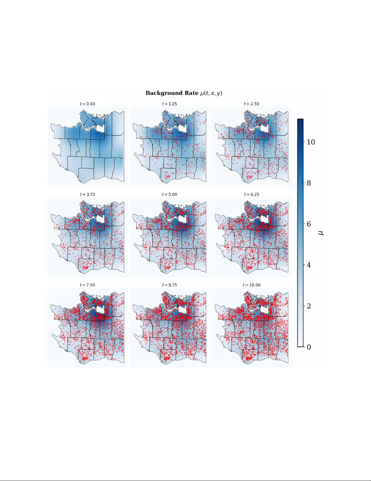
Fle xible and Scalable Ba y esian Modelling Of Spatio- T emporal Ha wk es Processes W enqing Liu ∗ 1 , Xenia Miscour idou † 2 , and Déborah Sulem ∗ 1 1 F aculty of Inf ormatics, U niversità della Svizzera italiana, Lug ano, Switzer land 2 Depar tment of Mathematics and S tatistics, Univ ersity of Cypr us, Nicosia, Cyprus Abstract Existing spatio-temporal Hawk es process models typically rely on either parametr ic or semiparametr ic assumptions, limiting the model’ s ability to capture complex endogenous and ex og enous e v ent dynamics. W e propose a fully Bay esian nonparametric frame work f or spatio-temporal Ha wkes processes using additive Gaussian processes f or the prior dis tr ibutions on the background rate and the tr igg er ing kernel. This additiv e str ucture enhances inter pretability by decoupling temporal and spatial eﬀects while maintaining high modelling ﬂexibility across the entire spatio-temporal domain. T o address scalability , we dev elop a sparse variational inference scheme based on the Gaussian v ariational famil y . Synthetic e xperiments demonstrate that the proposed method accurately reco vers back ground and tr igg er ing structures, achie ving superior per f or mance compared to exis ting alter nativ es. When applied to real-wor ld datasets, it achiev es higher held-out log-likelihoods and rev eals inter pretable spatio-temporal structures of the self-e x citation mechanism. Ov erall, the frame w ork pro vides a ﬂe xible, scalable, inter pretable, and uncer tainty -a ware approach for modelling comple x e xcitation patter ns in spatio-temporal ev ent data. Ke yw ords: Ba y esian nonparametrics; Gaussian process; Ha wkes process; spatio-temporal modelling; v ariational inference. 1 Introduction Man y real-wor ld phenomena exhibit contagious beha viour, where ev ents cluster in both time and space. In seismology , ma jor earthquakes are typicall y follo w ed b y aftershock sequences concentrated near the epicenter and shor tl y after the main shock [ Ogata , 1988 , 1998 ]. In cr iminology , bur glary incidents often e xhibit “near -repeat" victimisation, where one crime triggers additional oﬀenses in nearby areas within a shor t per iod [ Mohler et al. , 2011 ]. Similar spatio-temporal clustering has been obser v ed in ter rorism and armed conﬂict data, where initial attacks may precipitate cy cles of f ollo w-up violence [ W ang et al. , 2023 ]. These ex amples all share the f eature that the occur rence of one ev ent increases the likelihood of subsequent e v ents nearb y in space and time. This character is tic, often ref er red to as self-e x citation, means that past ev ents increase the probability of future ev ents. Ha wk es processes [ Hawk es , 1971 ] provide a general framew ork f or modelling such history-dependent dynamics of ev ents occur rences. They represent the conditional intensity as the sum of a background rate, captur ing ex ogenous inﬂuences, and a tr igg er ing kernel that descr ibes ho w past ev ents increase the likelihood of a future ev ent. By e xtending this f or mulation to incorporate spatial dependence, spatio-temporal Hawk es processes model ho w both the timing and the locations of past ev ents ∗ Emails: wenqing.liu@usi.ch , deborah.sulem@usi.ch † Email: miscouridou.xenia@ucy.ac.cy 1 jointl y shape the r isk of future ev ents, and hav e become a standard tool for studying e v ent data that e xhibit clustering and contagion eﬀects. While the Ha wk es model is conceptuall y ﬂe xible, practical implementations typically impose s trong assumptions on the f or ms of its main components, the bac kground rate and the tr igg ering kernel. As a result, most spatio-temporal Hawk es processes rely on speciﬁed parametr ic f orms f or these components. T emporal triggering k ernels are typically assumed to be exponential or po wer -law [ Bernabeu et al. , 2025 ] whereas spatial kernels are often taken to be Gaussian [ Miscour idou et al. , 2023 ]. Further more, most Ha wkes processes in literature assume a constant background rate [ Ber nabeu et al. , 2025 , Ha wkes , 1971 ], thereby ignor ing the temporal or spatial variation coming from ex ogenous factors. All the af orementioned assumptions facilitate inf erence but res tr ict the ﬂexibility of the model, and may prev ent it from captur ing complex temporal trends, spatial heterog eneity , and interactions betw een temporal and spatial coordinates that are often present in real-w orld ev ent data. T o o vercome the limitations of parametr ic spatio-temporal Ha wk es processes, the background rate and the triggering kernel should ideally be modelled with ﬂexible, data-dr iv en functional f or ms rather than res tr icted to ﬁxed parametr ic shapes. A Ba y esian nonparametric formulation naturally provides this ﬂe xibility through priors that allow the functions to vary freely while quantifying uncer tainty in the estimated spatio-temporal structure. At the same time, fully nonparametric Ba y esian models req uire poster ior inf erence o v er a v ast latent space that scales with both data size and dimensionality , rendering them computationall y prohibitiv e in larg e-scale spatio-temporal settings, which makes scalability an essential practical consideration. Further more, our frame work is computationall y scalable to larg e spatio-temporal point patterns thanks to a v ar iational appro ximation. Theref ore, w e propose a nov el fully Ba y esian nonparametric spatio-temporal Ha wk es process that satisﬁes both ﬂexibility and scalability requirements with the f ollowing contr ibutions: (1) W e model both the background rate and the tr igg er ing kernel in a full y Bay esian nonparametric wa y using Gaussian process (GP) pr iors. Exis ting spatio-temporal Ha wkes processes typically impose parametr ic f or ms on at least one of these components; this entirel y nonparametric Bay esian framew ork allo w s the data to determine temporal and spatial structure while pro viding uncer tainty quantiﬁcation. (2) W e emplo y an additive GP representation f or both components of the Hawk es process. This additive structure increases inter pretability b y modelling temporal, spatial, and cross-dimensional interaction eﬀects separatel y rather than f orcing them into a single joint kernel. Bey ond inter pretability , we empir icall y obser v e that the additiv e f or mulation typicall y enhances numerical s tability and perf orms at least as w ell as its non-additiv e alter nativ e. (3) W e perform poster ior inf erence using a variational Gaussian appro ximation (V GA) built on a sparse GP representation of the latent components of the Hawk es process. V GA along with the sparse GP enables eﬃcient optimisation and computational scalability . (4) W e ev aluate our frame w ork using various link functions and GP kernels across both synthetic and real-wor ld datasets, whereas exis ting Bay esian nonparametric temporal Hawk es methods are typically restricted to speciﬁc link functions f or conjugacy . This demonstrates the v ersatility of our framew ork in suppor ting div erse model speciﬁcations. The remainder of this paper is organised as follo w s. Section 2 revie ws related w ork, Section 3 presents the proposed methodology , Section 4 validates the per f or mance on both synthetic and real-wor ld data, and Section 5 oﬀers a discussion and conclusion. 2 R elated methods In purely temporal settings, Ha wkes processes hav e been used to model complex point patterns [ Hawk es , 1971 , Sulem et al. , 2022 , 2024 ]. Their e xtension to the spatio-temporal domain has receiv ed increasing attention in recent years due to their ability to capture self-e x citing phenomena across both dimensions. This 2 modelling framew ork has been applied in various ﬁelds, including ﬁnance [ Bacr y et al. , 2015 , Chen et al. , 2022 ], neuroscience [ Johnson , 1996 ], cr iminology [ Mohler et al. , 2011 ], epidemiology [ Chiang et al. , 2022 ], and seismology [ Ogata , 1998 , Kwon et al. , 2023 ]. Se v eral recent sur v e y s provide broader o v er vie ws of these de v elopments. In par ticular , Ber nabeu Atanasio et al. [ 2024 ] f ocuses on recent methodological advances, while Reinhart [ 2018 ] co vers f oundational aspects along with applications across multiple domains. Most classical spatio-temporal Hawk es processes adopt a fully parametr ic speciﬁcation, in which both the background rate and the tr igg er ing kernel are described by ﬁx ed functional f or ms. The back ground rate is often modeled as constant [ Schoenberg , 2023 , Ber nabeu et al. , 2025 ], while the triggering kernel is typicall y taken to be separable, with exponential deca y ov er time and Gaussian spread ov er space, such as in [ Miscour idou et al. , 2023 , Ber nabeu Atanasio et al. , 2024 , Mohler , 2014 ]. Such parametr ic f or mulations oﬀer inter pretability and computational tractability , but their f or m can be inadequate f or captur ing comple x or ir regular spatio-temporal patter ns often obser v ed in real-w orld data. R elaxing these assumptions, a line of work has e xplored nonparametric modelling of the intensity within a Bay esian frame w ork, most notably via log-Gaussian Co x processes. In these models, a GP pr ior is placed on a latent log-intensity , which is then mapped to the positiv e domain through an exponential or sigmoid link function to ensure non-negativity [ Møller et al. , 1998 , Samo and Roberts , 2015 ]. In the conte xt of Hawk es processes, Miscouridou et al. [ 2023 ] proposed the Cox–Ha wkes model, which uses a log-Gaussian Co x process pr ior f or the background rate while retaining parametr ic e xponential and Gaussian kernels f or the triggering kernel. This hybrid design introduces nonparametr ic ﬂe xibility f or the baseline but still relies on strong structural assumptions f or the e x citation mechanism. P osterior inference is per f or med using MCMC, aided by pre-trained GP generators to accelerate sampling. Alaimo Di Loro et al. [ 2025 ] proposed a semi-parametr ic Hawk es process model, which treats the back ground component nonparametrically b y estimating its spatio-temporal varying intensity directly on the road network, while preser ving a structured f or m f or the e x citation mechanism. This frame work utilises a stoc hastic-recons tr uction algor ithm that iterativ el y updates the background r isk through empir ical smoothing of ev ents, rather than assuming a ﬁx ed parametr ic baseline. By combining this ﬂexible back ground with a parametric tr igg er ing component, the model eﬀectiv ely balances local data adaptability with the interpretability of self-ex citation patter ns. A diﬀerent approach is tak en b y Zhou et al. [ 2020 ], who proposed a fully nonparametric temporal Ha wk es model by placing GP pr iors on both the background rate and the tr igg er ing kernel. A sigmoid link function is used not onl y to enf orce positivity but also, when combined with suitable latent v ariables, to achie ve conjugacy that enables a range of inf erence schemes, including EM algor ithms, Gibbs sampling, and v ariational inference (VI). While this frame w ork av oids parametric assumptions on the tr igg er ing kernel and captures r ic h temporal dynamics, it is limited to purely temporal data and is tightly coupled to the sigmoid link function. Extending it to a general spatio-temporal setting would require latent-variable updates o v er a high-dimensional space, causing the computational cost to g ro w prohibitiv el y . Ov erall, the method is diﬃcult to extend directly to the spatio-temporal domain or to accommodate alter nativ e link functions. While the method of Zhou et al. [ 2020 ] represents a Bay esian nonparametric direction, a substantial literature on frequentist nonparametric estimation f or Ha wkes processes has also emerg ed. Maximum- likelihood-based methods ha v e been de v eloped to estimate tr igg er ing kernels and, in some cases, bac kground rates in a ﬂe xible manner [ Marsan and Lengline , 2008 , Lewis and Mohler , 2011 , Zhou et al. , 2013 ]. These approaches are attractiv e due to their eﬃciency and asymptotic proper ties, but they yield point estimates rather than full distr ibutions, and theref ore do not provide uncer tainty quantiﬁcation for the inf er red intensity components. From a Bay esian perspective, posterior inf erence is often car ried out using Mark o v Chain Monte Carlo (MCMC) algorithms [ A dams et al. , 2009 , Donnet et al. , 2020 , Miscour idou et al. , 2023 ], which oﬀer principled uncer tainty quantiﬁcation but can be computationally demanding, par ticular ly f or larg e spatio-temporal 3 datasets. VI has emerg ed as a scalable alternative, pro viding approximate posterior distributions at a fraction of the computational cost [ Malem-Shinitski et al. , 2021 , Sulem et al. , 2022 , Zhou et al. , 2020 ]. Theoretical guarantees for such Ba y esian nonparametric f or mulations in the spatio-temporal domain hav e also been established, including results on posterior contraction rates [ Miscour idou and Sulem , 2026 ]. Ho we ver , man y e xisting VI approaches rely on independence assumptions that factorise the posterior o ver latent variables, potentiall y limiting the ability to capture complex posterior dependencies. This motivates the use of more e xpressive appro ximations, such as the Gaussian variational famil y , which w e adopt in this w ork. Ov erall, these factors indicate the need to fur ther relax parametric assumptions while maintaining scalability in Ha wk es process modelling. How ev er , exis ting methods either (i) maintain parametr ic structure in at least one component, (ii) remain conﬁned to purel y temporal settings, or (iii) lack a fully Ba yesian treatment that is both nonparametric and scalable in space and time. Our work ﬁlls these gaps by proposing a no vel fully Ba yesian nonparametric spatio-temporal Hawk es model in which both the background rate and the tr igg ering kernel are modelled with GP pr iors, and a scalable VI algorithm is used to appro ximate the posterior . 3 Methodology 3.1 Problem Setup W e assume that we obser v e a spatio-temporal point process 𝑁 on a bounded domain W = T × S , where T = [ 0 , 𝑇 ] is the temporal window , 𝑇 > 0 is the time hor izon, and S ⊂ R 𝑑 is the spatial domain. T ypical choices include 𝑑 = 1 f or a single spatial coordinate, 𝑑 = 2 f or planar settings, and 𝑑 = 3 f or applications such as latitude-longitude-depth. The data consists of one or multiple realisations of this point process 𝑁 . F or clarity , w e ﬁrst consider that we only obser v e one sequence of points { ( 𝑡 𝑖 , 𝑠 𝑖 ) } 𝑛 𝑖 = 1 with 𝑡 𝑖 ∈ T and 𝑠 𝑖 ∈ S . Let H 𝑡 = { ( 𝑡 𝑖 , 𝑠 𝑖 ) : 𝑡 𝑖 < 𝑡 } denote the history up to time 𝑡 . The la w of this process is speciﬁed b y its conditional intensity . For eac h ( 𝑡 , 𝑠 ) ∈ W , the conditional intensity , given the histor y H 𝑡 , of a Hawk es process is 𝜆 ( 𝑡 , 𝑠 | H 𝑡 ) = 𝜇 ( 𝑡 , 𝑠 ) +  𝑡 𝑖 <𝑡 𝜙  𝑡 − 𝑡 𝑖 , 𝑠 − 𝑠 𝑖  , (1) where 𝜇 ( 𝑡 , 𝑠 ) ≥ 0 is the bac k g r ound r ate representing e x ogenous ar rivals, and 𝜙 ( Δ 𝑡 , Δ 𝑠 ) ≥ 0 is the trigg ering kernel character izing the endogenous self-ex citing eﬀect, where Δ 𝑡 = 𝑡 − 𝑡 𝑖 and Δ 𝑠 = 𝑠 − 𝑠 𝑖 denote the relativ e time and spatial lags from a past ev ent, respectiv el y . The cumulative impact of these tw o components can be characterised by their respectiv e 𝐿 1 -norms. Speciﬁcally , the total expected number of background ev ents within the obser v ation domain W is given b y : ∥ 𝜇 ∥ 1 =  S  T 𝜇 ( 𝑡 , 𝑠 ) d 𝑡 d 𝑠 , (2) Mean while, the o v erall strength of the self-e x citation is summar ised b y the branching ratio, deﬁned as the 𝐿 1 -norm of 𝜙 ov er its suppor t: ∥ 𝜙 ∥ 1 =  S  ∞ 0 𝜙 ( Δ 𝑡 , Δ 𝑠 ) d Δ 𝑡 d Δ 𝑠 . (3) The branching ratio ∥ 𝜙 ∥ 1 represents the e xpected number of oﬀspring e v ents g enerated b y a single ev ent. T o ensure the process is stable, i.e., does not e xplode, w e assume the stationarity condition ∥ 𝜙 ∥ 1 < 1 [ Bernabeu Atanasio et al. , 2024 , Siviero et al. , 2024 , R einhart , 2018 , Miscour idou et al. , 2023 ]. U nder this condition, the total e xpected number of ev ents in the bounded domain W can be approximated as E [ 𝑁 ( W ) ] ≈ ∥ 𝜇 ∥ 1 / ( 1 − ∥ 𝜙 ∥ 1 ) [ Miscouridou et al. , 2023 ] with 𝑁 (W the number of ev ents in W . A detailed derivation of this appro ximation is provided in Appendix A . 4 3.2 Gaussian Process Prior T o ﬂexibl y model both the background rate 𝜇 and the tr igg er ing kernel 𝜙 , we introduce latent functions 𝑓 𝜇 and 𝑓 𝜙 and apply link functions to ensure non-negativity . Speciﬁcall y , the conditional intensity of a Ha wk es process in ( 1 ) is ref ormulated as 𝜆 ( 𝑡 , 𝑠 | H 𝑡 ) = ℎ 𝜇  𝑓 𝜇 ( 𝑡 , 𝑠 )  +  𝑡 𝑖 <𝑡 ℎ 𝜙  𝑓 𝜙 ( 𝑡 − 𝑡 𝑖 , 𝑠 − 𝑠 𝑖 )  (4) where ℎ 𝜇 , ℎ 𝜙 : R → R ≥ 0 are ﬁxed, non-negativ e, bijectiv e and non-decreasing link functions, suc h as the softplus [ Mei and Eisner , 2017 , Sulem et al. , 2022 ], sigmoid [ Zhou et al. , 2020 , Malem-Shinitski et al. , 2021 ], or exponential functions [ Møller et al. , 1998 , Diggle et al. , 2013 , Miscour idou et al. , 2023 ]. The latent functions 𝑓 𝜇 and 𝑓 𝜙 are given independent Gaussian process pr iors, 𝑓 𝜇 ( 𝑡 , 𝑠 ) ∼ G P ( 𝜂 𝜇 , 𝐾 𝜇 ) , 𝑓 𝜙 ( Δ 𝑡 , Δ 𝑠 ) ∼ G P ( 𝜂 𝜙 , 𝐾 𝜙 ) where 𝑓 𝜇 is deﬁned on absolute coordinates ( 𝑡 , 𝑠 ) , while 𝑓 𝜙 is deﬁned on temporal and spatial lags ( Δ 𝑡 , Δ 𝑠 ) = ( 𝑡 − 𝑡 𝑖 , 𝑠 − 𝑠 𝑖 ) with Δ 𝑡 ≥ 0 . A bo ve, 𝜂 𝜇 and 𝜂 𝜙 denote the GP mean functions, which are assumed to be zero without loss of generality [ Zhou , 2019 ]. The cov ar iance kernels 𝐾 𝜇 and 𝐾 𝜙 encode pr ior beliefs about the smoothness and cor relation s tructures of the latent functions. W e pr imarily emplo y stationary f amilies such as the squared-e xponential (RBF) or Matér n [ Williams and Rasmussen , 2006 ], parameterised b y a signal variance 𝜎 2 (controlling amplitude) and lengthscales ℓ (controlling cor relation ranges). For the spatio-temporal domain, w e consider both traditional separable kernels which factorise into independent spatial and temporal components 𝐾 separable  ( 𝑡 , 𝑠 ) , ( 𝑡 ′ , 𝑠 ′ )  = 𝜎 2 𝑘 𝑡 ( 𝑡 , 𝑡 ′ | 1 , ℓ 𝑡 ) 𝑘 𝑠 ( 𝑠 , 𝑠 ′ | 1 , ℓ 𝑠 ) , (5) and a more inter pretable additiv e framew ork [ Plate , 1999 , Duvenaud et al. , 2011 ], where marginal and interaction eﬀects are explicitl y modelled to capture cross-dimensional dependencies 𝐾 additiv e  ( 𝑡 , 𝑠 ) , ( 𝑡 ′ , 𝑠 ′ )  = 𝑘 𝑡 ( 𝑡 , 𝑡 ′ | 𝜎 2 𝑡 , ℓ 𝑡 ) + 𝑘 𝑠 ( 𝑠 , 𝑠 ′ | 𝜎 2 𝑠 , ℓ 𝑠 ) + 𝑘 𝑡 , 𝑠  ( 𝑡 , 𝑠 ) , ( 𝑡 ′ , 𝑠 ′ ) | 𝜎 2 𝑡 , 𝑠 , ℓ 𝑡 , 𝑠  . (6) Mathematical deﬁnitions for all kernels are provided in Appendix B . 3.3 Model Likelihood W e no w specialise to the tw o-dimensional spatial case ( 𝑑 = 2 ). F or simplicity , let W = [ 0 , 𝑇 ] × [ 0 , 𝑋 ] × [ 0 , 𝑌 ] with 𝑋 , 𝑌 > 0 and D = { ( 𝑡 𝑖 , 𝑥 𝑖 , 𝑦 𝑖 ) } 𝑛 𝑖 = 1 denote the observed sequence of e v ents on W . F ollo wing Daley and V ere-Jones [ 2008 ], the likelihood of a spatio-temporal Ha wkes process is: 𝑝 ( D | 𝜇 , 𝜙 ) =  𝑛  𝑖 = 1 𝜆 ( 𝑡 𝑖 , 𝑥 𝑖 , 𝑦 𝑖 | H 𝑡 𝑖 )  e xp  −  W 𝜆 ( 𝑡 , 𝑥 , 𝑦 | H 𝑡 ) dt dx dy  . (7) For 𝑀 independent sequences { D ( 𝑚 ) = { ( 𝑡 ( 𝑚 ) 𝑖 , 𝑥 ( 𝑚 ) 𝑖 , 𝑦 ( 𝑚 ) 𝑖 ) } 𝑛 𝑚 𝑖 = 1 } 𝑀 𝑚 = 1 , the joint likelihood is the product of the likelihoods of each sequence: 𝑝 ( { D ( 𝑚 ) } 𝑀 𝑚 = 1 | 𝜇, 𝜙 ) = 𝑀  𝑚 = 1   𝑛 𝑚  𝑖 = 1 𝜆  𝑡 ( 𝑚 ) 𝑖 , 𝑥 ( 𝑚 ) 𝑖 , 𝑦 ( 𝑚 ) 𝑖 | H ( 𝑚 ) 𝑡 𝑖   e xp  −  W 𝜆 ( 𝑡 , 𝑥 , 𝑦 | H ( 𝑚 ) 𝑡 ) dt dx dy   . Ev aluating the likelihood in ( 7 ) is computationall y demanding for nonparametric models. U nlik e parametric tr igg er ing kernels, which often admit closed-f orm integrals, a nonparametric tr igg er ing kernel 5 modelled b y a GP requires e xplicit computation o v er histor y . Without structural restrictions, each e vent depends on all previous ev ents, resulting in quadratic comple xity in the number of obser v ations. T o reduce this burden, w e follo w [ Sulem et al. , 2024 , Zhou et al. , 2020 ] and assume the tr igg er ing kernel 𝜙 has ﬁnite suppor t Ω 𝜙 = [ 0 , 𝑇 𝜙 ] × [ − 𝑋 𝜙 , 𝑋 𝜙 ] × [ − 𝑌 𝜙 , 𝑌 𝜙 ] , with 𝑇 𝜙 , 𝑋 𝜙 , 𝑌 𝜙 > 0 , vanishing else where. U nder this assumption, only recent ev ents within the suppor t contr ibute to the intensity and the integral, reducing both computations to linear comple xity . This assumption is empirically justiﬁed, as inﬂuence is typically localised in domains like neuroscience [ Staerman et al. , 2023 , Eichler et al. , 2017 ], ﬁnance [ Bacr y et al. , 2015 , Car reira , 2021 ], and cr iminology [ Zhou et al. , 2020 ]. U nder this assumption, the likelihood ( 7 ) simpliﬁes to the form der iv ed in Appendix C : 𝑝 ( D | 𝜇 , 𝜙 ) = e xp  −  𝑇 0  𝑋 0  𝑌 0 𝜇 ( 𝑡 , 𝑥 , 𝑦 ) dt dx dy  × exp  − 𝑛  𝑖 = 1  min ( 𝑇 𝜙 , 𝑇 − 𝑡 𝑖 ) 0  min ( 𝑋 𝜙 , 𝑋 − 𝑥 𝑖 ) max ( − 𝑋 𝜙 , − 𝑥 𝑖 )  min ( 𝑌 𝜙 , 𝑌 − 𝑦 𝑖 ) max ( − 𝑌 𝜙 , − 𝑦 𝑖 ) 𝜙 ( Δ 𝑡 , Δ 𝑥 , Δ 𝑦 ) d Δ t d Δ x d Δ y  × 𝑛  𝑖 = 1    𝜇 ( 𝑡 𝑖 , 𝑥 𝑖 , 𝑦 𝑖 ) +  𝑗 : 𝑡 𝑗 <𝑡 𝑖 𝜙 ( Δ 𝑡 𝑖 𝑗 , Δ 𝑥 𝑖 𝑗 , Δ 𝑦 𝑖 𝑗 )    . (8) where Δ 𝑡 𝑖 𝑗 = 𝑡 𝑖 − 𝑡 𝑗 , Δ 𝑥 𝑖 𝑗 = 𝑥 𝑖 − 𝑥 𝑗 , and Δ 𝑦 𝑖 𝑗 = 𝑦 𝑖 − 𝑦 𝑗 . 3.4 Inf erence Ha ving established the expression of the likelihood, our goal is to perf orm Bay esian inf erence f or the back ground rate 𝜇 and the tr igg er ing kernel 𝜙 from the obser v ed ev ents D . Follo wing the non parametric frame w ork established in Section 3.2 , we do not place pr iors directly on 𝜇 and 𝜙 . Instead, these components are modelled as transf or mations of latent Gaussian processes, i.e., 𝜇 = ℎ 𝜇 ( 𝑓 𝜇 ) and 𝜙 = ℎ 𝜙 ( 𝑓 𝜙 ) . Conseq uentl y , the inference problem translates to estimating these latent functions 𝑓 = { 𝑓 𝜇 , 𝑓 𝜙 } and hyperparameters 𝜃 = { 𝜃 𝜇 , 𝜃 𝜙 } of the GP kernels. The speciﬁc joint poster ior distribution o v er these latent functions is: 𝑝 ( 𝑓 𝜇 , 𝑓 𝜙 , 𝜃 𝜇 , 𝜃 𝜙 | D ) ∝ 𝑝 ( D | 𝑓 𝜇 , 𝑓 𝜙 ) 𝑝 ( 𝑓 𝜇 | 𝜃 𝜇 ) 𝑝 ( 𝑓 𝜙 | 𝜃 𝜙 ) 𝑝 ( 𝜃 𝜇 ) 𝑝 ( 𝜃 𝜙 ) . (9) where 𝑝 ( 𝑓 | 𝜃 ) denotes the GP pr ior and 𝑝 ( 𝜃 ) the h yper prior (f or background or tr igg er ing k er nel components). For practical computation, the latent functions 𝑓 𝜇 and 𝑓 𝜙 are e v aluated on a ﬁnite discretisation grid. Speciﬁcall y , f or 𝑓 𝜇 , the gr id has 𝑛 𝜇 , 𝑡 points in time and 𝑛 𝜇 , 𝑥 , 𝑛 𝜇 , 𝑦 points in space, giving a total number of points of 𝑁 𝜇 = 𝑛 𝜇 , 𝑡 × 𝑛 𝜇 , 𝑥 × 𝑛 𝜇 , 𝑦 . The g rid for 𝑓 𝜙 has 𝑛 𝜙 , 𝑡 , 𝑛 𝜙 , 𝑥 , 𝑛 𝜙 , 𝑦 points in each dimension, resulting in 𝑁 𝜙 = 𝑛 𝜙 , 𝑡 × 𝑛 𝜙 , 𝑥 × 𝑛 𝜙 , 𝑦 gr id points. Direct inf erence on this speciﬁc posterior ( 9 ) is intractable due to the non-conjugate relationship between the Hawk es likelihood and the Gaussian process pr iors. While Mark o v Chain Monte Carlo (MCMC) methods can theoretically yield e xact samples from the poster ior , they are computationally prohibitiv e due to the dimensionality of the discretised latent functions. Consequently , we adopt variational inference [ Jordan et al. , 1999 , Blei et al. , 2017 ] to achie v e scalability and eﬃciency . The goal of variational inf erence is to appro ximate the intractable posterior 𝑝 ( 𝑓 𝜇 , 𝑓 𝜙 , 𝜃 𝜇 , 𝜃 𝜙 | D ) in ( 9 ) . A variational famil y Q is introduced to pro vide a tractable set of candidate densities ov er the latent variables, deﬁned on the same domain as the posterior distribution. The variational distr ibution 𝑞 ( 𝑓 𝜇 , 𝑓 𝜙 , 𝜃 𝜇 , 𝜃 𝜙 ) ∈ Q is chosen to minimise the Kullbac k –Leibler (KL) diver g ence to the tr ue posterior . Finding this optimal 𝑞 is equiv alent to maximising the Evidence Lo w er Bound (ELBO): L ( 𝑞 ) = E 𝑞  log 𝑝 ( 𝑓 𝜇 , 𝑓 𝜙 , 𝜃 𝜇 , 𝜃 𝜙 , D )  − E 𝑞  log 𝑞 ( 𝑓 𝜇 , 𝑓 𝜙 , 𝜃 𝜇 , 𝜃 𝜙 )  . (10) 6 A detailed der iv ation demonstrating this equiv alence is provided in Appendix D . The choice of the variational f amil y Q is cr itical for the quality of posterior approximation. In the present setting, the latent functions 𝑓 𝜇 and 𝑓 𝜙 are modelled as GPs, and it is therefore essential that the v ariational f amil y preser v es the cor relation structure within each latent process while remaining computationally tractable. W e adopt a V ar iational Gaussian Appro ximation (V GA) [ Opper and Archambeau , 2009 , Zhou , 2019 ] with the block -wise factorisation: 𝑞 ( 𝑓 𝜇 , 𝑓 𝜙 , 𝜃 𝜇 , 𝜃 𝜙 ) = 𝑞 ( 𝑓 𝜇 , 𝜃 𝜇 ) 𝑞 ( 𝑓 𝜙 , 𝜃 𝜙 ) (11) which assumes independence betw een the background and triggering components. Within each block, an additional factorisation is used: 𝑞 ( 𝑓 𝜇 , 𝜃 𝜇 ) = 𝑞 ( 𝑓 𝜇 ) 𝑞 ( 𝜃 𝜇 ) , 𝑞 ( 𝑓 𝜙 , 𝜃 𝜙 ) = 𝑞 ( 𝑓 𝜙 ) 𝑞 ( 𝜃 𝜙 ) . (12) This independence betw een the latent function and its h yperparameters is introduced f or eﬃciency . The v ariational distributions ov er the latent functions are chosen as multivariate Gaussians: 𝑞 ( 𝑓 𝜇 ) = N ( 𝑚 𝜇 , Σ 𝜇 ) , 𝑞 ( 𝑓 𝜙 ) = N ( 𝑚 𝜙 , Σ 𝜙 ) . (13) The full co variance matrices Σ 𝜇 and Σ 𝜙 preserve the dependence betw een function values, allowing the v ariational distributions to reﬂect the smoothness structure induced b y the GP pr iors. It is impor tant to retain dependencies within the hyperparameters of each latent process. Since the h yperparameters 𝜃 of the GP kernels are positiv e, we deﬁne the variational appro ximation in the log-domain. Speciﬁcall y , w e assign multiv ariate Gaussian distributions to the log-transf ormed hyperparameters 𝛼 𝜇 = log 𝜃 𝜇 and 𝛼 𝜙 = log 𝜃 𝜙 : 𝑞 ( 𝛼 𝜇 ) = N ( 𝑚 𝜃 𝜇 , Σ 𝜃 𝜇 ) , 𝑞 ( 𝛼 𝜙 ) = N ( 𝑚 𝜃 𝜙 , Σ 𝜃 𝜙 ) (14) impl ying that 𝑞 ( 𝜃 𝜇 ) and 𝑞 ( 𝜃 𝜙 ) f ollow multivariate Log-nor mal distributions: 𝑞 ( 𝜃 𝜇 ) = L N ( 𝑚 𝜃 𝜇 , Σ 𝜃 𝜇 ) , 𝑞 ( 𝜃 𝜙 ) = L N ( 𝑚 𝜃 𝜙 , Σ 𝜃 𝜙 ) (15) The use of full co variance matr ices Σ 𝜃 𝜇 and Σ 𝜃 𝜙 allo ws the variational distr ibution to capture potential cor relations betw een hyperparameters [ Flaxman et al. , 2015 ], enabling the model to represent dependencies that may ar ise in the posterior . 3.5 Sparse GP Appro ximation U nder the V G A s tr ucture deﬁned in Equations ( 11 ) – ( 12 ) , calculating the KL div ergence between the v ariational distributions 𝑞 ( 𝑓 𝜇 ) , 𝑞 ( 𝑓 𝜙 ) and the pr iors 𝑝 ( 𝑓 𝜇 ) , 𝑝 ( 𝑓 𝜙 ) requires the inv ersion of the kernel matr ices 𝐾 𝜇 and 𝐾 𝜙 . In our spatio-temporal setting, the sizes of these matr ices are respectiv el y 𝑁 𝜇 × 𝑁 𝜇 and 𝑁 𝜙 × 𝑁 𝜙 and are typicall y so larg e that these matr ix operations, which scale as O ( 𝑁 3 𝜇 + 𝑁 3 𝜙 ) , become computationally inf easible. T o ensure scalability , a sparse GP appro ximation is adopted follo wing Titsias [ 2009 ], replacing each full GP with a low er -rank inducing-point representation and substantially reducing the cost of ELBO optimisation. For the background component, let 𝑍 𝜇 = { 𝑧 𝑚 } 𝑀 𝜇 𝑚 = 1 ⊂ [ 0 , 𝑇 ] × [ 0 , 𝑋 ] × [ 0 , 𝑌 ] be a set of inducing locations, and deﬁne the inducing variables u 𝜇 : = 𝑓 𝜇 ( 𝑍 𝜇 ) ∈ R 𝑀 𝜇 . U nder the GP pr ior 𝑝 ( u 𝜇 ) = N ( 0 , 𝐾 𝑍 𝜇 𝑍 𝜇 ) , where 𝐾 𝑍 𝜇 𝑍 𝜇 ∈ R 𝑀 𝜇 × 𝑀 𝜇 is the kernel matr ix ev aluated at the inducing locations. The tr igg er ing component is handled analogously using inducing locations 𝑍 𝜙 = { z 𝑛 } 𝑀 𝜙 𝑛 = 1 ⊂ [ 0 , 𝑇 𝜙 ] × [ − 𝑋 𝜙 , 𝑋 𝜙 ] × [ − 𝑌 𝜙 , 𝑌 𝜙 ] and the cor responding inducing variables u 𝜙 = 𝑓 𝜙 ( 𝑍 𝜙 ) . 7 T o select the inducing variables, w e adopt the approach of [ Zhou et al. , 2020 ], where the inducing locations 𝑍 𝜇 and 𝑍 𝜙 are placed on equidistant gr ids o ver their respective domains. Giv en the inducing variables, the latent functions at the gr id locations are recov ered via Gaussian conditioning [ Titsias , 2009 , Zhou , 2019 ]. For the background latent function 𝑓 𝜇 , 𝑝 ( 𝑓 𝜇 | u 𝜇 ) = N ( 𝑚 𝑓 | 𝑢 𝜇 , Σ 𝑓 | 𝑢 𝜇 ) , with 𝑚 𝑓 | 𝑢 𝜇 = 𝐾 𝑍 𝑍 𝜇 𝐾 − 1 𝑍 𝜇 𝑍 𝜇 u 𝜇 , (16) Σ 𝑓 | 𝑢 𝜇 = 𝐾 𝑍 𝑍 − 𝐾 𝑍 𝑍 𝜇 𝐾 − 1 𝑍 𝜇 𝑍 𝜇 𝑘 𝑍 𝜇 𝑍 . (17) U nder our variational Gaussian appro ximation, the variational posterior on the inducing variables is 𝑞 ( u 𝜇 ) = N ( 𝜇 𝜇 , 𝑆 𝜇 ) , 𝑞 ( u 𝜙 ) = N ( 𝜇 𝜙 , 𝑆 𝜙 ) . The variational posteriors ov er the latent functions are obtained b y marginalizing out the inducing variables: 𝑞 ( 𝑓 𝜇 ) =  𝑝 ( 𝑓 𝜇 | u 𝜇 ) 𝑞 ( u 𝜇 ) 𝑑 u 𝜇 , 𝑞 ( 𝑓 𝜙 ) =  𝑝 ( 𝑓 𝜙 | u 𝜙 ) 𝑞 ( u 𝜙 ) 𝑑 u 𝜙 . Since both ter ms are Gaussian and conjugate, the marginals remain Gaussian with closed-f orm e xpressions. For 𝑓 𝜇 , 𝑞 ( 𝑓 𝜇 ) = N  ˜ 𝑚 𝜇 , ˜ Σ 𝜇  , where ˜ 𝑚 𝜇 and ˜ Σ 𝜇 are given b y [ Lloyd et al. , 2015 ], with the der iv ation provided in Appendix E , ˜ 𝑚 𝜇 = 𝐾 𝑍 𝑍 𝜇 𝐾 − 1 𝑍 𝜇 𝑍 𝜇 𝜇 𝜇 , (18) ˜ Σ 𝜇 = 𝐾 𝑍 𝑍 − 𝐾 𝑍 𝑍 𝜇 𝐾 − 1 𝑍 𝜇 𝑍 𝜇 𝐾 𝑍 𝜇 𝑍 + 𝐾 𝑍 𝑍 𝜇 𝐾 − 1 𝑍 𝜇 𝑍 𝜇 𝑆 𝜇 𝐾 − 1 𝑍 𝜇 𝑍 𝜇 𝐾 𝑍 𝜇 𝑍 . (19) W e can inter pret the f or m of ˜ Σ 𝜇 as f ollo w s: the ﬁrst ter m 𝐾 𝑍 𝑍 represents the original GP pr ior uncer tainty , while the second ter m, 𝐾 𝑍 𝑍 𝜇 𝐾 − 1 𝑍 𝜇 𝑍 𝜇 𝐾 𝑍 𝜇 𝑍 , cor responds to the par t of this uncer tainty that can be explained b y the inducing variables, so their diﬀerence captures the remaining uncer tainty that the inducing variables cannot represent [ Quinonero-Candela and Rasmussen , 2005 ]. The ﬁnal ter m, 𝐾 𝑍 𝑍 𝜇 𝐾 − 1 𝑍 𝜇 𝑍 𝜇 𝑆 𝜇 𝐾 − 1 𝑍 𝜇 𝑍 𝜇 𝐾 𝑍 𝜇 𝑍 , adds back the uncer tainty arising from the fact that the inducing variables themselv es are not known e xactl y but hav e an appro ximate posterior with cov ar iance 𝑆 𝜇 . The e xpressions for 𝑞 ( 𝑓 𝜙 ) are analogous. Although the sparse construction pro vides closed-form variational posteriors 𝑞 ( 𝑓 𝜇 ) and 𝑞 ( 𝑓 𝜙 ) , these distributions are still deﬁned ov er all latent function ev aluations, and their co v ariance matr ices remain dense with sizes 𝑁 𝜇 × 𝑁 𝜇 and 𝑁 𝜙 × 𝑁 𝜙 . Consequentl y , computing ELBO ter ms that require sampling from 𝑞 ( 𝑓 𝜇 ) or 𝑞 ( 𝑓 𝜙 ) in v olv es operations on these dense co variance matr ices, necessitating a Cholesky decomposition with O ( 𝑁 3 𝜇 ) or O ( 𝑁 3 𝜙 ) comple xity . This computational burden motivates the additional appro ximations introduced belo w . W e adopt the Deter minis tic T raining Conditional (DTC) approximation [ Quinonero-Candela and Ras- mussen , 2005 , Hensman et al. , 2018 ], in which the latent function 𝑓 ∗ 𝜇 is based on the projection: 𝑓 ∗ 𝜇 = 𝐾 𝑍 𝑍 𝜇 𝐾 − 1 𝑍 𝜇 𝑍 𝜇 u 𝜇 , u 𝜇 ∼ 𝑞 ( u 𝜇 ) = N ( 𝜇 𝜇 , 𝑆 𝜇 ) . The poster ior mean follo w s directly from the linear mapping: 𝑚 ∗ 𝜇 = E [ 𝑓 ∗ 𝜇 ] = 𝐾 𝑍 𝑍 𝜇 𝐾 − 1 𝑍 𝜇 𝑍 𝜇 𝜇 𝜇 . 8 The cov ar iance is Σ ∗ 𝜇 = Co v  𝑓 ∗ 𝜇  = 𝐾 𝑍 𝑍 𝜇 𝐾 − 1 𝑍 𝜇 𝑍 𝜇 𝑆 𝜇 𝐾 − 1 𝑍 𝜇 𝑍 𝜇 𝐾 𝑍 𝜇 𝑍 . In DTC, the pr ior residual ter m 𝐾 𝑍 𝑍 − 𝑘 𝑍 𝑍 𝜇 𝐾 − 1 𝑍 𝜇 𝑍 𝜇 𝐾 𝑍 𝜇 𝑍 present in the full sparse posterior is omitted. As this residual ter m vanishes when the inducing set becomes the or iginal g rid, the DTC approximation impro v es with larg er numbers of inducing variables, consistent with the classical Nys tröm appro ximation [ Williams and Seeg er , 2000 ]. The same appro ximation is applied to the posterior on the triggering kernel’ s latent function. In this sparse approximation setting, the poster ior distribution in ( 9 ) can be wr itten as 𝑝 ( 𝑓 ∗ 𝜇 , 𝑓 ∗ 𝜙 , u 𝜇 , u 𝜙 , 𝜃 𝜇 , 𝜃 𝜙 | D ) ∝ 𝑝  D | 𝜇 = ℎ 𝜇 ( 𝑓 ∗ 𝜇 ) , 𝜙 = ℎ 𝜙 ( 𝑓 ∗ 𝜙 )  𝑝 ( 𝑓 ∗ 𝜇 | u 𝜇 , 𝜃 𝜇 ) 𝑝 ( 𝑓 ∗ 𝜙 | u 𝜙 , 𝜃 𝜙 ) × 𝑝 ( u 𝜇 ) 𝑝 ( u 𝜙 ) 𝑝 ( 𝜃 𝜇 ) 𝑝 ( 𝜃 𝜙 ) . (20) Since 𝑓 ∗ 𝜇 and 𝑓 ∗ 𝜙 are conditionally recov ered from the inducing v ar iables, the variational dis tribution onl y needs to be deﬁned ov er the inducing v alues and the hyperparameters, 𝑞 ( u 𝜇 , u 𝜙 , 𝜃 𝜇 , 𝜃 𝜙 ) . The cor responding ELB O in ( 10 ) is L ( 𝑞 ) = E 𝑞  log 𝑝 ( 𝑓 ∗ 𝜇 , 𝑓 ∗ 𝜙 , u 𝜇 , u 𝜙 , 𝜃 𝜇 , 𝜃 𝜙 , D )  − E 𝑞  log 𝑞 ( u 𝜇 , u 𝜙 , 𝜃 𝜇 , 𝜃 𝜙 )  . (21) In summary , the sparse GP appro ximation introduces inducing variables to obtain a lo w-rank representation of each GP prior, while the DTC approximation fur ther simpliﬁes the variational posterior by projecting all latent function e v aluations onto these inducing variables. This combination yields a scalable v ar iational inf erence scheme f or spatio-temporal Hawk es processes. 4 Experiments 1 Detailed h yper parameter settings, gr id resolutions, and computational conﬁgurations used in our experiments are provided in Appendix F . 4.1 Baselines and Metrics W e compare our model against sev eral spatio-temporal Ha wkes process baselines, which are estimated using v ariational inference f or consistency with our approach. Parame tric Ha wk es Process [ Bernabeu et al. , 2025 ]: The back ground rate 𝜇 is assumed constant and the triggering kernel takes the parametr ic f or m: 𝛼 𝛽 2 𝜋 𝜎 𝑥 𝜎 𝑦 e xp  − 𝛽 ( 𝑡 − 𝑡 𝑖 )  e xp  − ( 𝑥 − 𝑥 𝑖 ) 2 2 𝜎 2 𝑥 − ( 𝑦 − 𝑦 𝑖 ) 2 2 𝜎 2 𝑦  (22) with hyperparameters 𝛼 , 𝛽 , 𝜎 𝑥 , 𝜎 𝑦 > 0 . 1 The model implementation can be f ound at https://github.com/Wenqing- Liu- 1010/ Flexible- and- Scalable- Bayesian- Modeling- Of- Spatio- Temporal- Hawkes- Processes . 9 Co x–Ha wk es Process [ Miscouridou et al. , 2023 ]: The back ground rate 𝜇 ( 𝑡 , 𝑥 , 𝑦 ) is modelled using a log-Gaussian Cox process, while the tr igg ering kernel retains the same parametr ic f orm as ( 22 ) . Although their GP pr ior consists of an additive RBF kernel with separate temporal and spatial components, here f or consistency w e adopt the interaction-aw are additive structure described in Section 3.2 . A ke y limitation of both baselines is their reliance on tr igg er ing kernels with exponential deca y and Gaussian f orms, which are inherently unsuitable f or captur ing non-monotonic tr igg er ing patter ns. T o ev aluate model per f or mance, w e emplo y the f ollo wing metr ics, with detailed mathematical formulations provided in Appendix F .1 : P osterior Mean Error ( 𝑃 𝑀 mse ): The mean squared er ror betw een the posterior mean estimates ˆ 𝜇 , ˆ 𝜙 and the g round tr uth. P osterior Expected Error ( 𝑃 𝐸 mse ): The e xpected mean squared er ror calculated under the v ar iational posterior distribution of 𝜇 and 𝜙 . Expected Log-Lik elihood ( 𝐸 𝐿 𝐿 ): The expected log-likelihood of the obser v ed data under the variational posterior . This metr ic ser v es as a measure of model ﬁt f or real-wor ld datasets. 4.2 Synthetic Data Experiments For synthetic data e xperiments, e vents are generated using a cluster -based simulation [ Miscouridou et al. , 2023 , Ber nabeu et al. , 2025 ] in a spatio-temporal domain ( 𝑇 , 𝑋 , 𝑌 ) = ( 10 , 10 , 10 ) . F or the tr igg ering kernel, w e set ( 𝑇 𝜙 , 𝑋 𝜙 , 𝑌 𝜙 ) = ( 0 . 5 , 0 . 3 , 0 . 3 ) . W e consider the follo wing three synthetic scenar ios, with increasing comple xity: Scenario 1. 𝜇 ( 𝑡 , 𝑥 , 𝑦 ) = 4 . 5 , 𝜙 ( Δ 𝑡 , Δ 𝑥 , Δ 𝑦 ) = 5 e xp  − ( Δ 𝑥 2 + Δ 𝑦 2 ) / 0 . 02  e xp ( − Δ 𝑡 ) . Scenario 2. 𝜇 ( 𝑡 , 𝑥 , 𝑦 ) = ( 1 . 5 + sin ( 2 𝜋 𝑡 / 𝑇 ) ) + ( 1 . 5 + sin ( 2 𝜋𝑥 / 𝑋 ) ) + ( 1 . 5 + sin ( 2 𝜋 𝑦 / 𝑌 ) ) , 𝜙 ( Δ 𝑡 , Δ 𝑥 , Δ 𝑦 ) = 5 e xp  − ( Δ 𝑥 2 + Δ 𝑦 2 ) / 0 . 02  e xp ( − Δ 𝑡 ) . Scenario 3. 𝜇 ( 𝑡 , 𝑥 , 𝑦 ) = ( 1 . 5 + sin ( 2 𝜋 𝑡 / 𝑇 ) ) + ( 1 . 5 + sin ( 2 𝜋𝑥 / 𝑋 ) ) + ( 1 . 5 + sin ( 2 𝜋 𝑦 / 𝑌 ) ) + sin ( 2 𝜋 𝑡 / 𝑇 ) sin ( 2 𝜋 𝑥 / 𝑋 ) sin ( 2 𝜋 𝑦 / 𝑌 ) , 𝜙 ( Δ 𝑡 , Δ 𝑥 , Δ 𝑦 ) = ( 1 + 10 ( Δ 𝑡 / 𝑇 𝜙 ) ( 1 − Δ 𝑡 / 𝑇 𝜙 ) ) exp ( − ( Δ 𝑥 2 / 𝑋 2 𝜙 + Δ 𝑦 2 / 𝑌 2 𝜙 ) ) . The ﬁrst scenar io cor responds to a parametric Hawk es process with constant background rate. The second introduces an additiv e nonstationary bac kground rate that varies independentl y in time and space. The third has a background rate which is nonstationary , with additiv e and interaction ter ms and a tr igg er ing kernel whic h is non-monotonic. These scenar ios allow us to e v aluate our model under classical settings, time-v arying bac kground rate, and the most ﬂe xible scenar ios inv olving both nons tationary 𝜇 ( 𝑡 , 𝑥 , 𝑦 ) and non-monotonic 𝜙 ( Δ 𝑡 , Δ 𝑥 , Δ 𝑦 ) . T o assess the impact of pr ior speciﬁcations on the inference, we e v aluate our model across various conﬁgurations, including separable and additive RBF and Matér n kernels (with smoothness lev el 𝜈 = 2 . 5 ), as w ell as diﬀerent link functions (softplus, e xponential, and sigmoid 2 ). W e present the results f or these combinations f or Scenarios 1 to 3 in T ables 1 , 2 , and 3 , whic h report 𝑃 𝑀 mse ( 𝜇 ) , 𝑃 𝑀 mse ( 𝜙 ) , 𝑃 𝐸 mse ( 𝜇 ) , 2 The sigmoid link function is implemented as 𝜎 ( 𝑥 ) = 𝛼 / ( 1 + exp (− 𝑥 ) ) , where 𝛼 is set to a relativel y larg e constant to accommodate the scale of the targ et latent intensity . 10 and 𝑃 𝐸 mse ( 𝜙 ) computed against the ground-tr uth background rate and tr igg er ing kernel. Detailed results regarding diﬀerent smoothness lev els f or the Matér n kernels ( 𝜈 = 0 . 5 , 1 . 5 ) across all scenar ios are pro vided in T ables 7 , 8 , and G.3 of Appendix G . The variational posterior mean on the background rate ˆ 𝜇 ( 𝑡 , 𝑥 , 𝑦 ) and triggering kernel ˆ 𝜙 ( Δ 𝑡 , Δ 𝑥 , Δ 𝑦 ) , along with their g round-truth counter parts, are visualised in Figures 1 , 4 , and 7 at selected timestamps. Further more, Figures 2 , 5 , and 8 pro vide a 3D visualisation of the full posterior distributions f or these components, show casing the posterior mean, the g round tr uth, and the 95% credible inter v als (CIs) to illustrate the uncer tainty of our inf erence. All results are obtained under the additiv e kernel conﬁguration. T o quantify the temporal ev olution of these components, we compute the spatial av erag e for both the background rate and the tr igg er ing kernel. Speciﬁcall y , f or each variational posterior sample, we calculate the f ollo wing spatial a v erages o v er their respective domains: ¯ 𝜇 ( 𝑡 ) = 1 | S 𝜇 |  S 𝜇 𝜇 ( 𝑡 , 𝑥 , 𝑦 ) 𝑑𝑥 𝑑 𝑦 , ¯ 𝜙 ( Δ 𝑡 ) = 1 | S 𝜙 |  S 𝜙 𝜙 ( Δ 𝑡 , Δ 𝑥 , Δ 𝑦 ) 𝑑 Δ 𝑥 𝑑 Δ 𝑦 , (23) where S 𝜇 = [ 0 , 𝑋 ] × [ 0 , 𝑌 ] and S 𝜙 = [ − 𝑋 𝜙 , 𝑋 𝜙 ] × [ − 𝑌 𝜙 , 𝑌 𝜙 ] denote the spatial suppor t f or the background rate and tr igg er ing kernel, respectiv el y , with | S 𝜇 | and | S 𝜙 | representing their cor responding areas. Figures 3 , 6 , and 9 present the resulting posterior mean of these spatial av erages, the 95% CIs der iv ed from the posterior samples, and the cor responding g round-truth cur v es. The results in T ables 1 , 2 , and 3 summarise the per f ormance of our framew ork. In Scenar io 1, the Parametric Hawk es and Co x-Ha wkes models achiev e the best per f or mance with lo wer 𝑃 𝑀 mse and 𝑃 𝐸 mse than our model, as their speciﬁcations match the data-generating processes more closely . Ho w e v er , our proposed model yields estimates close to the g round tr uth. As illustrated in Figures 1 , 2 , and 3 , our poster ior mean estimates reco v er the steady , in variant back ground rate and point-source diﬀusion patter ns (Fig. 1 ), while 3D visualisations conﬁrm that the tr ue intensity sur f aces remain within the 95% CIs (Fig. 2 ). Notabl y , the model reco vers the constant background rate and the temporal deca y of the tr igg er ing kernel (Fig. 3 ). For Scenario 2, the results are presented in T able 2 and Figures 4 , 5 , and 6 . In this comple x setting, Parametric Hawk es model yields the poorest per f or mance due to the limitations of its predeﬁned functional f or ms. Although the Co x-Ha wkes model is the most closel y aligned with the tr ue data-generating process, our proposed nonparametric framew ork demonstrates comparable or ev en slightly superior per f or mance in cer tain metrics. As illustrated in Fig. 4 , the posterior mean estimates accurately capture the oscillating spatial intensity across diﬀerent time slices. This precision is fur ther conﬁr med b y the 3D sur f ace plots in Fig. 5 , where the estimated sur f aces (blue) closely ov erlap with the g round tr uth (green), with the tr ue intensity remaining well within the 95% CIs (g re y shaded area). Fig. 6 characterises the temporal ev olution of the spatial a v erages; the results clearl y demonstrate that our model captures the signiﬁcant ﬂuctuations in the back ground rate 𝜇 , with the posterior mean tightly tracking the trajectory of the ground truth while simultaneousl y reco v ering the deca y structure of the tr igg er ing kernel 𝜙 . The results f or Scenar io 3 are presented in T able 3 and Figures 7 , 8 , and 9 . In this scenar io, our model outperforms all baselines, achie ving the low est er rors across all metr ics. This per f ormance gap highlights the inherent limitations of parametr ic or semi-parametr ic baselines when confronted with complex dynamics. A ke y challeng e in Scenar io 3 is that the triggering kernel 𝜙 is non-monotonic o v er time, as clearl y sho wn in the r ight panel of Fig. 9 . Such a complex temporal structure is extremel y diﬃcult to capture using standard parametric functional f orms, which typically assume monotonic decay . In contrast, our fully nonparametric approach oﬀers superior ﬂexibility , allowing the posterior mean to accurately track this non-monotonic r ise and fall. Further more, Fig. 7 and F ig. 8 demonstrate that our model maintains high precision in estimating the spatio-temporal back ground rate 𝜇 . The 3D sur f ace plots conﬁr m that e v en under these highly dynamic 11 Figure 1: Estimated Hawk es process components f or Scenar io 1. The ﬁgure is divided into two main panels: the back ground rate 𝜇 ( 𝑡 , 𝑥 , 𝑦 ) (left) and the triggering kernel 𝜙 ( Δ 𝑡 , Δ 𝑥 , Δ 𝑦 ) (right), each sho wn at tw o diﬀerent time snapshots. F or each component, the ground tr uth is on the left and the poster ior mean estimate is on the right. conditions, the tr ue intensity sur f aces remain consistently within the 95% CIs, show casing the robustness of our framew ork in reco v er ing comple x Hawk es process components. In addition, the results across all scenar ios in T ables 1 , 2 , and 3 demonstrate that our additiv e kernels g enerall y outper f or m their separable counter parts, or at the v er y least e xhibit comparable per f or mance. This adv antag e is particularly evident in the bac kground rate estimation ( 𝑃 𝑀 mse ( 𝜇 ) and 𝑃 𝐸 mse ( 𝜇 ) ), while the performance on the tr igg er ing kernel 𝜙 remains comparable to that of the separable kernels. W e attr ibute this gain to the enhanced numerical s tability of the additiv e f or mulation. In sparse GP inf erence, the stability of inv er ting the inducing point cov ar iance matrices 𝐾 𝑍 𝜇 𝑍 𝜇 and 𝐾 𝑍 𝜙 𝑍 𝜙 depends on their condition number 𝜅 ( 𝐾 ) = 𝜆 max ( 𝐾 ) / 𝜆 min ( 𝐾 ) . Here 𝜆 max and 𝜆 min denote the maximum and minimum eigen values, respectivel y . As summar ised in T able 4 , which repor ts the condition numbers of 𝐾 𝑍 𝜇 𝑍 𝜇 and 𝐾 𝑍 𝜙 𝑍 𝜙 f or the separable and additiv e RBF kernels under the softplus link function, separable kernels generall y e xhibit higher condition numbers, leading to ill-conditioned matrices. In contrast, the additiv e structure brings low er condition numbers (or at least comparable ones), thereby ensur ing more robust estimation. 12 Figure 2: Three-dimensional visualisation of the estimated Hawk es process components f or Scenar io 1, including posterior uncertainty . Left: back ground rate 𝜇 ( 𝑡 , 𝑥 , 𝑦 ) at 𝑡 = 5 . Right: triggering kernel 𝜙 ( Δ 𝑡 , Δ 𝑥 , Δ 𝑦 ) at Δ 𝑡 = 0 . 25 . The plots sho w the variational posterior mean (blue), ground tr uth (green), and the 95% CIs (g re y shaded area). Figure 3: Spatial av erages of the Ha wkes process components f or Scenar io 1. Left: spatial a v erage of the back ground rate ov er its domain. Right: spatial a v erage of the triggering kernel o v er its domain. The plots sho w the variational posterior mean (blue), ground tr uth (green), and 95% CIs. 13 Figure 4: Estimated Hawk es process components for Scenar io 2. The background rate 𝜇 (left) and triggering kernel 𝜙 (right) are sho wn at diﬀerent time snapshots. For each component, the ground tr uth is on the left and the variational posterior mean estimate is on the r ight. Figure 5: Three-dimensional visualisation of the estimated Ha wk es process components f or Scenar io 2, demonstrating captured posterior uncer tainty . Left: background rate 𝜇 ( 𝑡 , 𝑥 , 𝑦 ) at 𝑡 = 5 . Right: triggering kernel 𝜙 ( Δ 𝑡 , Δ 𝑥 , Δ 𝑦 ) at Δ 𝑡 = 0 . 25 . The plots displa y the variational posterior mean (blue), g round truth (green), and the 95% CIs (g re y shaded area). 14 Figure 6: Spatial av erages of the Ha wkes process components f or Scenar io 2. Left: spatial a v erage of the back ground rate ov er its domain. Right: spatial a v erage of the triggering kernel o v er its domain. The plots sho w the variational posterior mean (blue), ground tr uth (green), and 95% CIs. Figure 7: Estimated Hawk es process components for Scenar io 3. The background rate 𝜇 (left) and triggering kernel 𝜙 (right) are shown at diﬀerent snapshots. For each component, the g round tr uth is on the left and the posterior mean estimate is on the r ight. 15 Figure 8: Three-dimensional visualisation of the estimated Ha wk es process components f or Scenar io 3, sho wing the posterior mean and associated uncer tainty . Left: back ground rate 𝜇 ( 𝑡 , 𝑥 , 𝑦 ) at 𝑡 = 5 . Right: triggering kernel 𝜙 ( Δ 𝑡 , Δ 𝑥 , Δ 𝑦 ) at Δ 𝑡 = 0 . 25 . The results illustrate the variational posterior mean (blue), ground tr uth (green), and the 95% CIs (grey shaded area). Figure 9: Spatial av erages of the Ha wkes process components f or Scenar io 3. Left: spatial a v erage of the back ground rate ov er its domain. Right: spatial a v erage of the triggering kernel o v er its domain. The plots sho w the variational posterior mean (blue), ground tr uth (green), and 95% CIs. 16 T able 1: Compar ison of diﬀerent methods f or Scenar io 1 using 𝑃 𝑀 mse ( 𝜇 ) , 𝑃 𝑀 mse ( 𝜙 ) , 𝑃 𝐸 mse ( 𝜇 ) , 𝑃 𝐸 mse ( 𝜙 ) . Method Link 𝑃 𝑀 mse ( 𝜇 ) 𝑃 𝑀 mse ( 𝜙 ) 𝑃 𝐸 mse ( 𝜇 ) 𝑃 𝐸 mse ( 𝜙 ) Parametric Ha wkes 1 . 21 ± 1 . 90 4 . 49 ± 2 . 26 1 . 90 ± 1 . 87 3 . 33 ± 0 . 47 Co x-Ha wkes e xp 4 . 63 ± 2 . 76 2 . 92 ± 1 . 66 13 . 84 ± 4 . 90 4 . 42 ± 1 . 66 Ours (separable RBF) softplus-softplus 8 . 13 ± 2 . 50 9 . 82 ± 2 . 31 14 . 95 ± 2 . 73 14 . 64 ± 2 . 42 Ours (separable RBF) sigmoid-sigmoid 8 . 03 ± 2 . 86 8 . 16 ± 2 . 26 15 . 96 ± 3 . 51 15 . 23 ± 2 . 12 Ours (separable RBF) e xp-e xp 8 . 48 ± 2 . 50 8 . 57 ± 1 . 97 16 . 29 ± 2 . 85 14 . 39 ± 2 . 12 Ours (separable Matérn, 𝜈 = 2 . 5 ) softplus-softplus 6 . 58 ± 2 . 08 7 . 36 ± 2 . 69 13 . 27 ± 2 . 24 12 . 03 ± 2 . 64 Ours (separable Matérn, 𝜈 = 2 . 5 ) sigmoid-sigmoid 7 . 34 ± 2 . 61 7 . 04 ± 2 . 32 15 . 13 ± 3 . 16 13 . 35 ± 2 . 28 Ours (separable Matérn, 𝜈 = 2 . 5 ) e xp-e xp 8 . 11 ± 2 . 69 8 . 12 ± 2 . 09 16 . 18 ± 3 . 19 14 . 01 ± 1 . 99 Ours (additiv e RBF) softplus-softplus 2 . 88 ± 0 . 88 5 . 01 ± 1 . 36 7 . 63 ± 0 . 82 10 . 16 ± 1 . 47 Ours (additiv e RBF) sigmoid-sigmoid 3 . 43 ± 1 . 20 7 . 91 ± 2 . 93 9 . 75 ± 1 . 50 15 . 43 ± 3 . 28 Ours (additiv e RBF) e xp-e xp 4 . 78 ± 2 . 22 7 . 26 ± 3 . 46 13 . 69 ± 4 . 23 14 . 08 ± 3 . 78 Ours (additiv e Matér n, 𝜈 = 2 . 5 ) softplus-softplus 3 . 14 ± 1 . 10 5 . 28 ± 1 . 77 8 . 44 ± 1 . 45 10 . 83 ± 1 . 93 Ours (additiv e Matér n, 𝜈 = 2 . 5 ) sigmoid-sigmoid 3 . 76 ± 1 . 51 7 . 55 ± 2 . 93 10 . 45 ± 2 . 06 14 . 62 ± 3 . 41 Ours (additiv e Matér n, 𝜈 = 2 . 5 ) e xp-e xp 5 . 11 ± 2 . 50 7 . 36 ± 2 . 31 13 . 82 ± 4 . 84 13 . 97 ± 2 . 31 The ﬁrst and second terms in the Link column refer to the link functions f or the background rate 𝜇 and the triggering kernel 𝜙 , respectiv ely . Results are av eraged ov er 8 independent realisations. Mean values and standard deviations ( ± ) are reported. R ed and blue indicate the best and second-best performance, respectiv el y . All values are scaled by 10 2 . T able 2: Compar ison of diﬀerent methods for Scenar io 2 based on 𝑃 𝑀 mse ( 𝜇 ) , 𝑃 𝑀 mse ( 𝜙 ) , 𝑃 𝐸 mse ( 𝜇 ) , 𝑃 𝐸 mse ( 𝜙 ) . Method Link 𝑃 𝑀 mse ( 𝜇 ) 𝑃 𝑀 mse ( 𝜙 ) 𝑃 𝐸 mse ( 𝜇 ) 𝑃 𝐸 mse ( 𝜙 ) Parametric Ha wkes 152 . 64 ± 3 . 24 16 . 78 ± 7 . 56 153 . 37 ± 3 . 26 11 . 58 ± 6 . 34 Co x-Ha wkes e xp 16 . 08 ± 4 . 72 4 . 21 ± 2 . 33 30 . 57 ± 6 . 09 5 . 68 ± 2 . 27 Ours (separable RBF) softplus-softplus 22 . 09 ± 7 . 26 13 . 24 ± 1 . 68 37 . 01 ± 6 . 70 18 . 04 ± 1 . 94 Ours (separable RBF) sigmoid-sigmoid 19 . 56 ± 5 . 97 11 . 76 ± 2 . 07 36 . 59 ± 5 . 88 19 . 24 ± 2 . 48 Ours (separable RBF) e xp-e xp 22 . 34 ± 6 . 55 11 . 58 ± 1 . 74 38 . 29 ± 6 . 21 17 . 71 ± 2 . 21 Ours (separable Matérn, 𝜈 = 2 . 5 ) softplus-softplus 18 . 16 ± 6 . 48 9 . 16 ± 1 . 43 31 . 73 ± 5 . 80 14 . 58 ± 1 . 89 Ours (separable Matérn, 𝜈 = 2 . 5 ) sigmoid-sigmoid 17 . 28 ± 5 . 91 10 . 14 ± 1 . 66 32 . 90 ± 5 . 69 16 . 91 ± 2 . 08 Ours (separable Matérn, 𝜈 = 2 . 5 ) e xp-e xp 18 . 62 ± 6 . 08 10 . 87 ± 1 . 36 33 . 69 ± 5 . 60 17 . 27 ± 1 . 80 Ours (additiv e RBF) softplus-softplus 11 . 14 ± 6 . 21 7 . 67 ± 1 . 37 20 . 22 ± 6 . 14 13 . 44 ± 2 . 74 Ours (additiv e RBF) sigmoid-sigmoid 11 . 95 ± 6 . 18 11 . 96 ± 2 . 58 22 . 88 ± 6 . 12 20 . 20 ± 3 . 56 Ours (additiv e RBF) e xp-e xp 14 . 12 ± 5 . 72 9 . 87 ± 1 . 91 25 . 52 ± 5 . 75 17 . 37 ± 3 . 16 Ours (additiv e Matér n, 𝜈 = 2 . 5 ) softplus-softplus 11 . 81 ± 6 . 14 8 . 08 ± 1 . 26 21 . 00 ± 5 . 86 14 . 48 ± 1 . 71 Ours (additiv e Matér n, 𝜈 = 2 . 5 ) sigmoid-sigmoid 12 . 38 ± 5 . 80 10 . 02 ± 1 . 85 23 . 27 ± 5 . 79 16 . 98 ± 2 . 55 Ours (additiv e Matér n, 𝜈 = 2 . 5 ) e xp-e xp 14 . 43 ± 6 . 22 10 . 50 ± 1 . 97 25 . 50 ± 6 . 44 18 . 26 ± 2 . 01 R esults are av eraged o v er 8 independent realisations. Mean values and standard deviations ( ± ) are repor ted. Red and blue indicate the best and second-best performance, respectiv el y . All values are scaled by 10 2 . 17 T able 3: Compar ison of diﬀerent methods for Scenar io 3 based on 𝑃 𝑀 mse ( 𝜇 ) , 𝑃 𝑀 mse ( 𝜙 ) , 𝑃 𝐸 mse ( 𝜇 ) , 𝑃 𝐸 mse ( 𝜙 ) . Method Link 𝑃 𝑀 mse ( 𝜇 ) 𝑃 𝑀 mse ( 𝜙 ) 𝑃 𝐸 mse ( 𝜇 ) 𝑃 𝐸 mse ( 𝜙 ) Parametric Ha wkes 169 . 55 ± 5 . 35 32 . 50 ± 4 . 42 170 . 35 ± 5 . 31 31 . 11 ± 3 . 81 Co x-Ha wkes e xp 24 . 39 ± 5 . 60 24 . 97 ± 1 . 46 47 . 32 ± 5 . 61 26 . 02 ± 1 . 44 Ours (separable RBF) softplus-softplus 22 . 92 ± 3 . 97 10 . 72 ± 5 . 46 41 . 49 ± 3 . 82 18 . 92 ± 4 . 71 Ours (separable RBF) sigmoid-sigmoid 25 . 24 ± 5 . 24 11 . 61 ± 5 . 07 47 . 67 ± 4 . 93 20 . 31 ± 4 . 94 Ours (separable RBF) e xp-e xp 28 . 08 ± 5 . 25 12 . 41 ± 5 . 29 48 . 23 ± 5 . 34 20 . 75 ± 4 . 68 Ours (separable Matérn, 𝜈 = 2 . 5 ) softplus-softplus 20 . 75 ± 3 . 86 10 . 23 ± 4 . 39 38 . 07 ± 3 . 80 18 . 74 ± 3 . 77 Ours (separable Matérn, 𝜈 = 2 . 5 ) sigmoid-sigmoid 23 . 00 ± 5 . 34 10 . 57 ± 5 . 20 43 . 84 ± 5 . 06 18 . 39 ± 4 . 84 Ours (separable Matérn, 𝜈 = 2 . 5 ) e xp-e xp 24 . 79 ± 5 . 32 11 . 75 ± 4 . 36 44 . 17 ± 5 . 43 20 . 18 ± 3 . 93 Ours (additiv e RBF) softplus-softplus 19 . 17 ± 5 . 28 10 . 14 ± 4 . 27 37 . 11 ± 4 . 42 18 . 54 ± 4 . 23 Ours (additiv e RBF) sigmoid-sigmoid 25 . 50 ± 4 . 14 9 . 31 ± 4 . 61 40 . 57 ± 8 . 14 17 . 49 ± 4 . 42 Ours (additiv e RBF) e xp-e xp 24 . 88 ± 6 . 60 9 . 26 ± 4 . 24 43 . 98 ± 6 . 32 17 . 84 ± 3 . 96 Ours (additiv e Matér n, 𝜈 = 2 . 5 ) softplus-softplus 18 . 27 ± 3 . 56 10 . 91 ± 5 . 89 37 . 76 ± 3 . 77 18 . 75 ± 5 . 45 Ours (additiv e Matér n, 𝜈 = 2 . 5 ) sigmoid-sigmoid 26 . 22 ± 4 . 27 9 . 70 ± 4 . 78 41 . 47 ± 8 . 80 17 . 94 ± 4 . 50 Ours (additiv e Matér n, 𝜈 = 2 . 5 ) e xp-e xp 25 . 32 ± 6 . 85 10 . 50 ± 4 . 39 45 . 91 ± 7 . 83 19 . 47 ± 4 . 47 R esults are av eraged o v er 8 independent realisations. Mean values and standard deviations ( ± ) are repor ted. Red and blue indicate the best and second-best performance, respectiv el y . All values are scaled by 10 2 . T able 4: Compar ison of condition numbers across diﬀerent synthetic scenar ios. 𝜅 ( 𝐾 𝑍 𝜇 𝑍 𝜇 ) and 𝜅 ( 𝐾 𝑍 𝜙 𝑍 𝜙 ) denote the condition numbers f or the background and tr igg er ing components, respectivel y . Lo w er condition numbers usually indicate better numer ical stability . Scenario Method Link 𝜅 ( 𝐾 𝑍 𝜇 𝑍 𝜇 ) 𝜅 ( 𝐾 𝑍 𝜙 𝑍 𝜙 ) Scenario 1 Ours (separable RBF) softplus-softplus 1 . 84 × 10 4 ± 1 . 02 × 10 4 1 . 79 × 10 2 ± 1 . 02 × 10 2 Ours (additiv e RBF) softplus-softplus 5 . 67 × 10 1 ± 5 . 09 × 10 0 4 . 84 × 10 1 ± 6 . 75 × 10 0 Scenario 2 Ours (separable RBF) softplus-softplus 4 . 92 × 10 4 ± 1 . 32 × 10 4 2 . 50 × 10 2 ± 6 . 67 × 10 1 Ours (additiv e RBF) softplus-softplus 1 . 37 × 10 2 ± 1 . 50 × 10 1 4 . 49 × 10 1 ± 7 . 74 × 10 0 Scenario 3 Ours (separable RBF) softplus-softplus 1 . 77 × 10 4 ± 1 . 05 × 10 4 1 . 96 × 10 2 ± 3 . 17 × 10 2 Ours (additiv e RBF) softplus-softplus 4 . 37 × 10 2 ± 3 . 48 × 10 2 3 . 51 × 10 2 ± 5 . 14 × 10 2 Mean and standard deviation ( ± ) of the condition numbers f or the induction points. V alues are multiplied b y 10 2 . 18 4.3 Real-w orld Data Experiments W e e valuate our nonparametric frame w ork on tw o real-wor ld spatio-temporal datasets: Chicago Shoot- ings [ Manr ing et al. , 2025 ] and V ancouv er Break -ins [ Zhou et al. , 2020 ]. Figure 10 illus trates the spatial distribution of e v ents f or both datasets. The Chicago Shootings dataset contains repor ted shooting incidents with continuous timestamps and g eographic coordinates. W e use the data from 2022 (2,124 ev ents) as the training seq uence and the data from 2023 (1,809 ev ents) f or testing. The V ancouver Break -ins dataset records break -and-enter incidents in V ancouv er . W e use the 2013 data (3,013 ev ents) f or training and the 2014 data (3,033 ev ents) for testing. For both datasets, we rescale the temporal dimension 𝑇 to [ 0 , 10 ] and the spatial coordinates ( 𝑋 , 𝑌 ) to [ 0 , 10 ] 2 . F or the Chicago Shootings dataset, the tr igg er ing kernel windo w is set to 𝑇 𝜙 = 0 . 4 (approximatel y half a month), with spatial windo w s 𝑋 𝜙 = 𝑌 𝜙 = 0 . 4 (representing ph ysical distances of approximatel y 1,278 m East- W est and 1,716.4 m North-South). For the V ancouv er Break -ins dataset, w e use 𝑇 𝜙 = 0 . 6 (appro ximately three weeks), with spatial windo w s 𝑋 𝜙 = 𝑌 𝜙 = 0 . 2 (representing phy sical distances of approximatel y 321.2 m East- W est and 233.6 m North-South). The selection of these ﬁnite windo w sizes is suppor ted by a sensitivity anal y sis detailed in Appendix H . Figure 10: Spatial distribution of ev ents in the real-wor ld datasets. Left: Chicago shooting incidents (2022 f or training and 2023 f or testing). Right: V ancouv er break -ins (2013 for training and 2014 for testing). The model ﬁt, ev aluated using the Expected Log-Likelihood ( 𝐸 𝐿 𝐿 ) on the test sets, is presented in T able 6 , with more comprehensiv e results f or all tested kernel and link function combinations pro vided in Appendix G.4 . Alongside standard baselines, we speciﬁcall y include a Log-Gaussian Co x Process [ Møller et al. , 1998 ] to isolate the impact of self-ex citation. Because the Log-Gaussian Cox Process models only the back ground rate without an y tr igg er ing mechanism, the fact that our proposed model yields a signiﬁcantly higher 𝐸 𝐿 𝐿 across both datasets pro vides strong evidence f or the presence of underl ying contagion eﬀects. Further more, among our proposed model variants, the additiv e kernel conﬁgurations yield the best o verall ﬁt. This sugg ests that decomposing the spatial and temporal components provides a better empir ical ﬁt f or these real-w orld ev ents. T o e v aluate goodness-of-ﬁt, we apply the super -thinning algor ithm [ Reinhart , 2018 ] (details in Ap- pendix I.1 ) to the estimated intensity obtained via the variational posterior mean on the bac kground rate 19 and triggering k er nel from our additiv e kernel conﬁgurations. After super -thinning, a perfectl y speciﬁed model yields a thinned process which has the distribution of a homogeneous Poisson process. W e assess the distribution of this thinned process using standard temporal and spatial diagnostics (see Appendix I.2 ). Our temporal diagnostics yield solid results. Kolmogoro v-Smirno v (KS) tests conﬁrm that the time betw een ev ents f ollow s the e xpected patter n. For the V ancouv er dataset, 16 out of 20 random seeds passed the test ( 𝑝 > 0 . 05 ). F or the Chicago dataset, the results were ev en more consistent, with 19 out of 20 seeds passing the test ( 𝑝 > 0 . 05 ). This high success rate across multiple independent r uns sugges ts that our temporal modeling is stable and per f or ms reliabl y . Spatiall y , ho we v er , visual inspection of the super -thinned ev ents (Figure 11 ) and subsequent quadrat count tests ( 𝑝 < 0 . 05 ) indicate the presence of residual localised clustering. This sugges ts that while our model eﬀectiv ely captures the temporal contagion and the primary spatial patterns, cer tain localised spatial heterogeneities remain unmodeled. This potential remaining cluster ing is likel y dr iv en b y external spatial cov ar iates that are not included in our model. Figure 11: Spatial distribution of the super -thinned e v ents. Left: Chicago shooting incidents. Right: V ancouver break -ins. Despite the minor spatial heterog eneities identiﬁed in the diagnostics, our Ba y esian framew ork pro vides the f ollowing inter pretable insights into the ov erall generating mechanisms of these e v ents. Note that in what f ollow s, all expected ev ent counts and their CIs are rounded to the nearest integer . For the Chicago Shootings dataset, the variational poster ior mean of the expected number of background ev ents is ∥ 𝜇 ∥ 1 = 1398 (95% CI: [ 1300 , 1500 ] ), and the branching ratio is ∥ 𝜙 ∥ 1 = 0 . 324 (95% CI: [ 0 . 278 , 0 . 382 ] ). Using the branching process identity E [ 𝑁 ( W ) ] ≈ ∥ 𝜇 ∥ 1 / ( 1 − ∥ 𝜙 ∥ 1 ) (see Appendix A f or the der iv ation), the implied e xpected number of total e v ents is 2073 (95% CI: [ 1876 , 2314 ] ). This aligns well with both the numer ical compensator estimate of 2131 (95% CI: [ 1992 , 2292 ] ) and the actual obser v ed number of training ev ents (2,124). With an estimated branching ratio of 0.324, we ﬁnd that nearl y a third of these shootings are directly tr igg ered by pre vious incidents within this windo w , highlighting a strong shor t-term contagion in urban gun violence. Similarl y , for the V ancouver Break -ins dataset, the variational posterior mean of the e xpected number of back ground ev ents is ∥ 𝜇 ∥ 1 = 2213 (95% CI: [ 2090 , 2346 ] ), with a branching ratio of ∥ 𝜙 ∥ 1 = 0 . 210 (95% CI: [ 0 . 176 , 0 . 248 ] ). The branching process identity yields an implied expected number of e v ents of 2804 (95% CI: [ 2610 , 3019 ] ), while the compensator yields 2904 (95% CI: [ 2741 , 3078 ] ). A gain, the true observed number of training ev ents (3,013) falls well within these CIs. Practicall y , a 21% branching ratio indicates that 20 within the chosen spatial-temporal window , localised near -repeat dynamics are responsible f or roughly one in ﬁv e break -ins. T o fur ther understand the behaviour of the additive kernel of the GP , we ex amine the v ar iational posterior means and 95% CIs of the hyperparameters for the additiv e kernel, which decomposes the underl ying Gaussian processes into purely temporal, purely spatial, and joint spatio-temporal components. T able 5: V ar iational posterior means and 95% CIs (in brack ets) f or the additiv e kernel hyperparameters. ℓ denotes the length scale and 𝜎 2 denotes the signal variance f or the temporal ( 𝑡 ), spatial ( 𝑠 ), and spatio-temporal ( 𝑡 , 𝑠 ) components. Length Scales ( ℓ ) Signal V ariance ( 𝜎 2 ) Dataset Component 𝑡 𝑠 ( 𝑡 , 𝑠 ) 𝑡 𝑠 ( 𝑡 , 𝑠 ) Chicago Background 𝜇 2.73 [1.46, 4.63] 2.07 [1.91, 2.23] 0.28 [0.12, 0.53] 0.82 [0.15, 2.41] 6.10 [3.84, 9.20] 0.47 [0.31, 0.67] T r igg er 𝜙 0.62 [0.11, 1.87] 0.04 [0.03, 0.05] 0.20 [0.16, 0.24] 0.26 [0.03, 0.89] 0.74 [0.43, 1.19] 0.93 [0.61, 1.37] V ancouver Background 𝜇 4.90 [2.24, 10.07] 1.23 [1.15, 1.31] 1.44 [1.15, 1.75] 2.78 [1.05, 6.04] 7.10 [4.57, 10.95] 1.44 [0.95, 2.13] T r igg er 𝜙 0.50 [0.06, 2.02] 0.02 [0.01, 0.02] 0.13 [0.10, 0.16] 0.39 [0.11, 1.08] 4.24 [3.12, 5.68] 2.36 [1.59, 3.32] While additive k ernels oﬀer inter pretable decompositions [ Duv enaud et al. , 2011 ] by measuring the signal variance ( 𝜎 2 ) of each ter m, they can suﬀer from identiﬁability issues [ Lu et al. , 2022 ]. T o address this, Or thogonal A dditive Kernels (O AK) were proposed [ Lu et al. , 2022 ]. Ho we v er , we do not emplo y O AK in this work, as the need to specify marginal data densities f or each dimension signiﬁcantl y complicates the modeling and increases the computational burden. Instead, w e verify the inter pretability of our model through empirical testing. A cross 20 random seeds, the lear ned h yperparameters f or the Chicago dataset w ere very similar . For the V ancouver dataset, all h yper parameters remained stable e x cept f or one temporal scale ( ℓ 𝑡 f or 𝜇 , which sho w ed two modes). This sugges ts that our model conv erg es to reliable optima rather than random local optima. Theref ore, giv en the stability of our results, our model’ s decomposition remains identiﬁable and inter pretable. Backgr ound Rate. When looking at the estimated background rate sur f aces ( 𝜇 ) (Figure 12 and Figure 13 ), w e obser v e distinct spatial hotspots that cor respond to areas with persistentl y high cr ime baseline rates. For Chicago, these hotspots are concentrated in certain neighbourhoods on the South and W est sides, while V ancouver sho w s elev ated background rates in speciﬁc do wnto wn area. As sho wn in T able 5 , In Chicago, the spatial factor is s tatisticall y robus t; its 95% CI lo wer bound ( 3 . 84 ) comf ortably e x ceeds the upper bounds of both the temporal ( 2 . 41 ) and spatio-temporal ( 0 . 67 ) components. This conﬁrms that Chicago’ s baseline crime risks are larg ely persistent and tied to long-term locational factors rather than temporal ﬂuctuations. For V ancouver , while the spatial v ariance remains the lar gest ( 𝜎 2 𝑠 = 7 . 10 ), its 95% CI o v erlaps with the temporal component ( 𝜎 2 𝑡 , upper bound 6 . 04 ). This sugges ts that while location is the strong est dr iv er, the baseline risk in V ancouv er is also inﬂuenced by broader temporal trends. Ov erall, these results indicate that while spatial persistence is a common f eature, the temporal stability of the background rate is more noticeable in the Chicago shootings dataset than in V ancouv er break -ins. T riggering Kernel. The poster ior means of the self-ex citation tr igg er ing kernels ( 𝜙 ) for the tw o datasets are shown in Figure 14 and Figure 15 in Appendix G.5 . W e obser v e that the tr igg ering eﬀects are strongl y centered in space and time in both cases. T able 5 fur ther highlights clear diﬀerences between shootings and break -ins. In Chicago, the tr igg ering eﬀect is mostl y dr iv en by the joint space-time component ( 𝜎 2 𝑠 𝑡 = 0 . 93 , 95% CI: [ 0 . 61 , 1 . 37 ] ). This means that retaliatory violence happens within a very speciﬁc windo w of both time and space. On the other hand, the spread of V ancouver break -ins is mos tl y driven by the pure spatial component ( 𝜎 2 𝑠 = 4 . 24 , 95% CI: [ 3 . 12 , 5 . 68 ] ). N otabl y , despite V ancouv er having a smaller phy sical triggering windo w than Chicago, it e xhibits a signiﬁcantly smaller spatial length scale ( ℓ 𝑠 = 0 . 02 , 95% CI: [ 0 . 01 , 0 . 02 ] vs. Chicago ’ s 0 . 04 , 95% CI: [ 0 . 03 , 0 . 05 ] ), indicating an ev en more localised concentration of 21 risk. This reﬂects the “near -repeat ” patter n inherent in burglar ies: once a proper ty is targ eted, the immediate neighbors face a higher r isk that is tied more to precise proximity than to a restrictive time windo w . These ﬁndings empirically conﬁr m that cr ime in the af orementioned datasets propagates similarl y to epidemic processes, meaning cr ime tr igg ers more cr ime. The highly localised spatial length scales f or both datasets underscore that cr ime contagion operates within a v ery restr icted microscopic radius. This sugges ts that future work f ocusing on inter v entions should treat cr ime spikes not merely as static non-contagious clusters, but as dynamic contagions, aiming to decrease the spread in space and time through rapid, geographically targ eted policing. T able 6: P erf ormance compar ison (Expected Log-Likelihood) on real-w or ld datasets. Chicago Shootings V ancouv er Break -ins Method Link 𝐸 𝐿 𝐿 Link 𝐸 𝐿 𝐿 Parametric Ha wkes Process – 1471 . 17 – 2203 . 65 Log Gaussian Co x Process exp 1535 . 49 e xp 2000 . 43 Co x-Ha wkes Process e xp 1647 . 26 e xp 2157 . 32 Ours (separable RBF) softplus-softplus 1615 . 71 softplus-softplus 2209 . 45 Ours (separable RBF) sigmoid-softplus 1642 . 24 sigmoid-softplus 2198 . 64 Ours (separable RBF) e xp-softplus 1643 . 36 e xp-softplus 2188 . 72 Ours (separable Matérn, 𝜈 = 2 . 5 ) softplus-softplus 1622 . 09 softplus-softplus 2220 . 85 Ours (separable Matérn, 𝜈 = 2 . 5 ) sigmoid-softplus 1645 . 43 sigmoid-softplus 2205 . 70 Ours (separable Matérn, 𝜈 = 2 . 5 ) e xp-softplus 1651 . 15 e xp-softplus 2193 . 20 Ours (additiv e RBF) softplus-softplus 1616 . 90 softplus-softplus 2249 . 02 Ours (additiv e RBF) sigmoid-softplus 1656 . 78 sigmoid-softplus 2245 . 78 Ours (additiv e RBF) e xp-e xp 1670 . 68 e xp-softplus 2227 . 90 Ours (additiv e Matér n, 𝜈 = 2 . 5 ) softplus-softplus 1621 . 99 softplus-softplus 2247 . 74 Ours (additiv e Matér n, 𝜈 = 2 . 5 ) sigmoid-softplus 1655 . 94 sigmoid-softplus 2241 . 56 Ours (additiv e Matér n, 𝜈 = 2 . 5 ) exp-e xp 1670 . 64 e xp-softplus 2215 . 98 Higher 𝐸 𝐿 𝐿 indicates super ior per f ormance. Best and second-best results in ter ms of 𝐸 𝐿 𝐿 are highlighted in red and blue, respectiv ely . 22 Figure 12: V ar iational posterior mean on the back ground rate at selected timestamps f or the Chicago shootings dataset (2022-2023) . 23 Figure 13: V ar iational posterior mean on the back ground rate at selected timestamps f or the V ancouv er break -ins dataset . 24 5 Discussion W e ha v e proposed a fully Ba y esian nonparametric framew ork f or spatio-temporal Hawk es processes, where both the background rate and the tr igg er ing kernel are modeled using Gaussian processes with ﬂexible co variance kernels. By lev eraging variational inf erence and sparse GP appro ximations, our method scales to large spatio-temporal point patter ns while retaining uncer tainty quantiﬁcation. Through comprehensive e xper iments on synthetic data with varying complexity , we demonstrated that our model can accurately recov er comple x spatial and temporal ex citation patter ns without imposing restrictive parametric assumptions. On real-w orld cr ime datasets (Chicago shootings and V ancouv er break -ins), our model consistentl y outper f or ms e xisting parametr ic baselines, achieving higher 𝐸 𝐿 𝐿 and pro viding inter pretable insights into the self-ex citing nature of cr iminal activities. Our ke y contr ibutions can be summarised as f ollo ws: (i) we introduce a nov el fully Bay esian nonparametric spatio-temporal Hawk es process model that ﬂe xibly captures both bac kground rate and tr igg ering k er nel; (ii) w e dev elop an eﬃcient variational inf erence algorithm with sparse GP appro ximations that scales to high-dimensional settings; (iii) w e demonstrate super ior per f or mance ov er state-of-the-ar t baselines on both synthetic and real-wor ld datasets; and (iv) w e provide inter pretable estimates of branching ratios and spatial hotspots that oﬀer actionable insights f or cr ime analy sis. Despite these strengths, se v eral limitations remain. Firs t, the cur rent model assumes a single e v ent type and ma y not capture interactions betw een diﬀerent ev ent categories. Second, our approach does not explicitl y incor porate e x og enous co variates that ma y inﬂuence ev ent rates. Thus, there exis t sev eral promising directions f or future w ork. Firs t, e xtending the frame work to multiv ariate Hawk es processes with both self-e x citation and cross-e xcitation between diﬀerent ev ent types w ould enable more nuanced modelling of complex phenomena such as the interaction betw een diﬀerent cr ime categories or betw een cr imes and their responses. Second, including e xternal cov ar iates in the model would allow us to better account for environmental factors and pro vide more detailed insights. Third, e xploring alternative nonparametric cons tructions such as neural netw ork -based intensity estimators could fur ther enhance model ﬂe xibility . In conclusion, the proposed frame w ork represents a signiﬁcant advance in ﬂe xible and scalable Bay esian nonparametric modelling of spatio-temporal Ha wkes processes, oﬀering both methodological contr ibutions and practical insights f or cr ime analy sis and bey ond. A ckno wledg ements W e ackno wledg e access to Piz Daint or Alps at the Swiss National Supercomputing Centre, Switzerland under the Univ ersità della Svizzera italiana ’ s share with the project ID u0. XM has received funding from the European Union ’ s Hor izon Europe research and innov ation programme under the Marie Sklodow ska-Cur ie g rant agreement 101151781 and from the Univ ersity of Cypr us under the startup grant prog ramme. 25 Appendix A Deriv ation of the Expected T otal Number of Ev ents T o deriv e the e xpected total number of ev ents E [ 𝑁 ( W ) ] using the branching process perspective, we can decompose the Ha wk es process into discrete generations of ev ents. Let 𝑁 𝑘 denote the number of e v ents in the 𝑘 -th generation within the spatial-temporal domain W = T × S . Firs t, the 0 -th generation consists solely of background ev ents (i.e., immigrants), which are g enerated independentl y b y the background rate 𝜇 ( 𝑡 , 𝑠 ) . The e xpected number of these background ev ents is the integ ral of the background rate ov er the domain: E [ 𝑁 0 ] =  W 𝜇 ( 𝑡 , 𝑠 ) d 𝑡 d 𝑠 = ∥ 𝜇 ∥ 1 . (24) Ne xt, each ev ent in the 0 -th g eneration acts as a parent, generating the 1 -st generation of oﬀspr ing ev ents. A ccording to the deﬁnition of the tr igg er ing kernel, the e xpected number of oﬀspr ing g enerated by a single e v ent is given b y the branching ratio ∥ 𝜙 ∥ 1 . Thus, the e xpected number of 1 -st generation ev ents is: E [ 𝑁 1 ] = E [ 𝑁 0 ] ∥ 𝜙 ∥ 1 = ∥ 𝜇 ∥ 1 ∥ 𝜙 ∥ 1 . (25) Follo wing this branching mechanism, the total number of ev ents in the 𝑘 -th g eneration, 𝑁 𝑘 , is the sum of oﬀspring g enerated b y the 𝑁 𝑘 − 1 parent ev ents from the previous generation. Given 𝑁 𝑘 − 1 , the conditional e xpectation of 𝑁 𝑘 is E [ 𝑁 𝑘 | 𝑁 𝑘 − 1 ] = 𝑁 𝑘 − 1 ∥ 𝜙 ∥ 1 , because each parent independently g enerates oﬀspr ing with an expected count of ∥ 𝜙 ∥ 1 . By applying the la w of total e xpectation, we can express the unconditional e xpectation of 𝑁 𝑘 as: E [ 𝑁 𝑘 ] = E  E [ 𝑁 𝑘 | 𝑁 𝑘 − 1 ]  = E  𝑁 𝑘 − 1 ∥ 𝜙 ∥ 1  = E [ 𝑁 𝑘 − 1 ] ∥ 𝜙 ∥ 1 . (26) By mathematical induction, appl ying this recursive relationship starting from E [ 𝑁 0 ] = ∥ 𝜇 ∥ 1 , the e xpected number of ev ents in the 𝑘 -th generation is: E [ 𝑁 𝑘 ] = ∥ 𝜇 ∥ 1 ∥ 𝜙 ∥ 𝑘 1 . (27) The total number of e vents in the domain W is the sum of e vents across all g enerations, giv en b y 𝑁 ( W ) =  ∞ 𝑘 = 0 𝑁 𝑘 . T aking the expectation on both sides yields: E [ 𝑁 ( W ) ] = E  ∞  𝑘 = 0 𝑁 𝑘  = ∞  𝑘 = 0 E [ 𝑁 𝑘 ] = ∞  𝑘 = 0 ∥ 𝜇 ∥ 1 ∥ 𝜙 ∥ 𝑘 1 = ∥ 𝜇 ∥ 1 ∞  𝑘 = 0 ∥ 𝜙 ∥ 𝑘 1 . (28) U nder the stationarity condition ∥ 𝜙 ∥ 1 < 1 , the inﬁnite geometric series con v erg es to 1 / ( 1 − ∥ 𝜙 ∥ 1 ) . Assuming the temporal and spatial boundar ies are suﬃciently larg e such that boundar y tr uncation eﬀects are negligible, we ar riv e at the ﬁnal approximation: E [ 𝑁 ( W ) ] ≈ ∥ 𝜇 ∥ 1 1 − ∥ 𝜙 ∥ 1 . (29) 26 B K ernel Functions In this section, we provide the detailed mathematical f or ms of the cov ar iance kernels. W e denote 𝑡 , 𝑡 ′ ∈ [ 0 , 𝑇 ] as temporal coordinates and 𝑠 , 𝑠 ′ ∈ [ 0 , 𝑋 ] × [ 0 , 𝑌 ] as spatial coordinates, with 𝑠 = ( 𝑥 , 𝑦 ) and 𝑠 ′ = ( 𝑥 ′ , 𝑦 ′ ) . Follo wing the deﬁnitions in Section 3.2 , each base kernel 𝑘 ( 𝑧 , 𝑧 ′ ) is parameter ised by a signal v ariance 𝜎 2 > 0 and lengthscale ℓ > 0 . Radial Basis Function (RBF) Kernel: The RBF kernel between tw o points 𝑧 and 𝑧 ′ is: 𝑘 RBF ( 𝑧 , 𝑧 ′ | 𝜎 2 , ℓ ) = 𝜎 2 e xp  − ∥ 𝑧 − 𝑧 ′ ∥ 2 2 ℓ 2  . (30) Matérn Kernels: The Matér n kernel with smoothness parameter 𝜈 ∈ { 0 . 5 , 1 . 5 , 2 . 5 } is: 𝑘 Mat ( 𝑧 , 𝑧 ′ | 𝜎 2 , 𝜈 , ℓ ) =              𝜎 2 e xp  − ∥ 𝑧 − 𝑧 ′ ∥ ℓ  , 𝜈 = 0 . 5 , 𝜎 2  1 + √ 3 ∥ 𝑧 − 𝑧 ′ ∥ ℓ  e xp  − √ 3 ∥ 𝑧 − 𝑧 ′ ∥ ℓ  , 𝜈 = 1 . 5 , 𝜎 2  1 + √ 5 ∥ 𝑧 − 𝑧 ′ ∥ ℓ + 5 ∥ 𝑧 − 𝑧 ′ ∥ 2 3 ℓ 2  e xp  − √ 5 ∥ 𝑧 − 𝑧 ′ ∥ ℓ  , 𝜈 = 2 . 5 . (31) B.1 Joint Kernel F orms Using the base kernels abov e, we deﬁne the speciﬁc joint spatio-temporal str uctures. Separable Joint Kernel: The separable kernel factorises the dependencies into independent marginal eﬀects, incor porating Automatic R ele v ance Deter mination (ARD) [ Liu et al. , 2020 ] o v er the temporal and spatial dimensions: 𝐾 separable  ( 𝑡 , 𝑠 ) , ( 𝑡 ′ , 𝑠 ′ )  = 𝜎 2 𝑘 𝑡 ( 𝑡 , 𝑡 ′ | 1 , ℓ 𝑡 ) 𝑘 𝑠 ( 𝑠 , 𝑠 ′ | 1 , ℓ 𝑥 , ℓ 𝑦 ) , (32) where 𝑘 𝑡 and 𝑘 𝑠 are base kernels deﬁned ov er the temporal and spatial domains, respectivel y , and 𝑠 = ( 𝑥 , 𝑦 ) . A common choice is the squared e xponential kernel: 𝐾 separable ( ( 𝑡 , 𝑠 ) , ( 𝑡 ′ , 𝑠 ′ ) ) = 𝜎 2 e xp  − ( 𝑡 − 𝑡 ′ ) 2 2 ℓ 2 𝑡 − ( 𝑥 − 𝑥 ′ ) 2 2 ℓ 2 𝑥 − ( 𝑦 − 𝑦 ′ ) 2 2 ℓ 2 𝑦  . (33) Alternativel y , with a Matér n-3/2 kernel, let 𝑠 =  𝑥 ℓ 𝑥 , 𝑦 ℓ 𝑦  , 𝑠 ′ =  𝑥 ′ ℓ 𝑥 , 𝑦 ′ ℓ 𝑦  . Then 𝐾 separable ( ( 𝑡 , 𝑠 ) , ( 𝑡 ′ , 𝑠 ′ ) ) = 𝜎 2  1 + √ 3 | 𝑡 − 𝑡 ′ | ℓ 𝑡  e xp  − √ 3 | 𝑡 − 𝑡 ′ | ℓ 𝑡   1 + √ 3 ∥ 𝑠 − 𝑠 ′ ∥  e xp  − √ 3 ∥ 𝑠 − 𝑠 ′ ∥  . (34) A dditiv e Joint Kernel: The additive kernel sums marginal temporal ( 𝑘 𝑡 ), marginal spatial ( 𝑘 𝑠 ), and joint interacton ( 𝑘 𝑡 , 𝑠 ) components: 𝐾 additiv e  ( 𝑡 , 𝑠 ) , ( 𝑡 ′ , 𝑠 ′ )  = 𝑘 𝑡 ( 𝑡 , 𝑡 ′ | 𝜎 2 𝑡 , ℓ 𝑡 ) + 𝑘 𝑠 ( 𝑠 , 𝑠 ′ | 𝜎 2 𝑠 , ℓ 𝑠 ) + 𝑘 𝑡 , 𝑠  ( 𝑡 , 𝑠 ) , ( 𝑡 ′ , 𝑠 ′ ) | 𝜎 2 𝑡 , 𝑠 , ℓ 𝑡 , 𝑠  , (35) where 𝑘 𝑠 is a 2D isotropic spatial kernel and 𝑘 𝑡 , 𝑠 is a 3D isotropic spatio-temporal kernel. 27 C Lik elihood derivation The likelihood 𝑝 ( D | 𝜇 , 𝜙 ) f or a spatio-temporal Hawk es process is deﬁned as: 𝐿 = e xp  −  𝑇 0  𝑋 0  𝑌 0 𝜆 ( 𝑡 , 𝑥 , 𝑦 | H 𝑡 ) dtdxdy  𝑛  𝑖 = 1 𝜆 ( 𝑡 𝑖 , 𝑥 𝑖 , 𝑦 𝑖 | H 𝑡 𝑖 ) . (36) By substituting the conditional intensity 𝜆 ( 𝑡 , 𝑥 , 𝑦 | H 𝑡 ) = 𝜇 ( 𝑡 , 𝑥 , 𝑦 ) +  𝑗 : 𝑡 𝑗 <𝑡 𝜙 ( 𝑡 − 𝑡 𝑗 , 𝑥 − 𝑥 𝑗 , 𝑦 − 𝑦 𝑗 ) , the product ov er obser v ed ev ents is e xpressed as: 𝑛  𝑖 = 1    𝜇 ( 𝑡 𝑖 , 𝑥 𝑖 , 𝑦 𝑖 ) +  𝑗 : 𝑡 𝑗 <𝑡 𝑖 𝜙 ( Δ 𝑡 𝑖 𝑗 , Δ 𝑥 𝑖 𝑗 , Δ 𝑦 𝑖 𝑗 )    . (37) The compensator ter m Λ =  W 𝜆 ( 𝑡 , 𝑥 , 𝑦 ) dtdxdy can be decomposed into background and tr igg er ing components, Λ 𝜇 + Λ 𝜙 . By sw apping the order of summation and integration f or the triggering par t, and appl ying the chang e of variables Δ 𝑡 = 𝑡 − 𝑡 𝑖 , Δ 𝑥 = 𝑥 − 𝑥 𝑖 , and Δ 𝑦 = 𝑦 − 𝑦 𝑖 , we obtain: Λ 𝜙 = 𝑛  𝑖 = 1  𝑇 𝑡 𝑖  𝑋 0  𝑌 0 𝜙 ( 𝑡 − 𝑡 𝑖 , 𝑥 − 𝑥 𝑖 , 𝑦 − 𝑦 𝑖 ) dtdxdy = 𝑛  𝑖 = 1  𝑇 − 𝑡 𝑖 0  𝑋 − 𝑥 𝑖 − 𝑥 𝑖  𝑌 − 𝑦 𝑖 − 𝑦 𝑖 𝜙 ( Δ 𝑡 , Δ 𝑥 , Δ 𝑦 ) d ( Δ t ) d ( Δ x ) d ( Δ y ) . (38) U nder the tr igg er ing kernel suppor t constraints ( 𝑇 𝜙 , 𝑋 𝜙 , 𝑌 𝜙 ) , the eﬀective integration limits f or each ev ent 𝑖 become: • Δ 𝑡 ∈ [ 0 , min ( 𝑇 𝜙 , 𝑇 − 𝑡 𝑖 ) ] • Δ 𝑥 ∈ [ max ( − 𝑋 𝜙 , − 𝑥 𝑖 ) , min ( 𝑋 𝜙 , 𝑋 − 𝑥 𝑖 ) ] • Δ 𝑦 ∈ [ max ( − 𝑌 𝜙 , − 𝑦 𝑖 ) , min ( 𝑌 𝜙 , 𝑌 − 𝑦 𝑖 ) ] Combining these components leads to the ﬁnal likelihood e xpression presented in Eq. ( 8 ). D V ariational inf erence VI appro ximates the intractable posterior 𝑝 ( 𝜃 | 𝐷 ) with a distribution 𝑞 ( 𝜃 ) from a tractable famil y Q that minimises the KL diver gence: 𝑞 ∗ ( 𝜃 ) = arg min 𝑞 ∈ Q KL ( 𝑞 ( 𝜃 ) ∥ 𝑝 ( 𝜃 | 𝐷 ) ) =  𝑞 ( 𝜃 ) log 𝑞 ( 𝜃 ) 𝑝 ( 𝜃 | 𝐷 ) 𝑑 𝜃 . (39) Using Bay es ’ r ule 𝑝 ( 𝜃 | 𝐷 ) = 𝑝 ( 𝐷 , 𝜃 ) / 𝑝 ( 𝐷 ) , the KL diver g ence can be expanded as: KL ( 𝑞 ( 𝜃 ) ∥ 𝑝 ( 𝜃 | 𝐷 ) ) =  𝑞 ( 𝜃 )  log 𝑞 ( 𝜃 ) 𝑝 ( 𝐷 , 𝜃 ) + log 𝑝 ( 𝐷 )  𝑑 𝜃 =  𝑞 ( 𝜃 ) log 𝑞 ( 𝜃 ) 𝑝 ( 𝐷 , 𝜃 ) 𝑑 𝜃 + log 𝑝 ( 𝐷 ) . (40) R e-ar ranging terms yields the decomposition of the marginal log-likelihood: log 𝑝 ( 𝐷 ) = L ( 𝑞 ) + KL ( 𝑞 ( 𝜃 ) ∥ 𝑝 ( 𝜃 | 𝐷 ) ) , (41) where L ( 𝑞 ) is the ELBO: L ( 𝑞 ) = E 𝑞 [ log 𝑝 ( 𝐷 , 𝜃 ) ] − E 𝑞 [ log 𝑞 ( 𝜃 ) ] = E 𝑞 [ log 𝑝 ( 𝐷 | 𝜃 ) ] − KL ( 𝑞 ( 𝜃 ) ∥ 𝑝 ( 𝜃 ) ) . (42) Since KL ( 𝑞 ∥ 𝑝 ) ≥ 0 , the ELBO pro vides a r igorous lo w er bound log 𝑝 ( 𝐷 ) ≥ L ( 𝑞 ) . Maximizing L ( 𝑞 ) with respect to 𝑞 is thus equiv alent to minimizing the KL div erg ence to the posterior . 28 E Deriv ation of the V ariational Marginal Distribution 𝑞 ( 𝑓 𝜇 ) Giv en the conditional distr ibution 𝑝 ( 𝑓 𝜇 | u 𝜇 ) = N ( 𝑚 𝑓 | 𝑢 𝜇 , Σ 𝑓 | 𝑢 𝜇 ) and the variational posterior o ver the inducing v ariables 𝑞 ( u 𝜇 ) = N ( 𝜇 𝜇 , 𝑆 𝜇 ) , the marginal distribution 𝑞 ( 𝑓 𝜇 ) is obtained by integ rating out u 𝜇 : 𝑞 ( 𝑓 𝜇 ) =  𝑝 ( 𝑓 𝜇 | u 𝜇 ) 𝑞 ( u 𝜇 ) d u 𝜇 . (43) Since this is a linear Gaussian sys tem, the resulting marginal distribution 𝑞 ( 𝑓 𝜇 ) is also Gaussian, denoted as N ( ˜ 𝑚 𝜇 , ˜ Σ 𝜇 ) . W e can der iv e its mean and co v ariance using the law of total e xpectation and the law of total v ariance, respectivel y . Deriv ation of the Mean ˜ 𝑚 𝜇 : By the law of total e xpectation, the unconditional mean is the expectation of the conditional mean: ˜ 𝑚 𝜇 = E 𝑞 ( u 𝜇 )  E [ 𝑓 𝜇 | u 𝜇 ]  = E 𝑞 ( u 𝜇 )  𝐾 𝑍 𝑍 𝜇 𝐾 − 1 𝑍 𝜇 𝑍 𝜇 u 𝜇  . (44) Since 𝐾 𝑍 𝑍 𝜇 𝐾 − 1 𝑍 𝜇 𝑍 𝜇 is a deter ministic matrix independent of u 𝜇 , we can factor it out of the expectation: ˜ 𝑚 𝜇 = 𝐾 𝑍 𝑍 𝜇 𝐾 − 1 𝑍 𝜇 𝑍 𝜇 E 𝑞 ( u 𝜇 ) [ u 𝜇 ] = 𝐾 𝑍 𝑍 𝜇 𝐾 − 1 𝑍 𝜇 𝑍 𝜇 𝜇 𝜇 . (45) Deriv ation of the Co variance ˜ Σ 𝜇 : By the law of total variance, the unconditional variance is the sum of the expected conditional variance and the variance of the conditional mean: ˜ Σ 𝜇 = E 𝑞 ( u 𝜇 )  V ar ( 𝑓 𝜇 | u 𝜇 )     T er m 1 + V ar 𝑞 ( u 𝜇 )  E [ 𝑓 𝜇 | u 𝜇 ]     T er m 2 . (46) For T erm 1, the conditional co variance Σ 𝑓 | 𝑢 𝜇 = 𝐾 𝑍 𝑍 − 𝐾 𝑍 𝑍 𝜇 𝐾 − 1 𝑍 𝜇 𝑍 𝜇 𝐾 𝑍 𝜇 𝑍 is deterministic and does not depend on the random variable u 𝜇 . Thus, its e xpectation is simply itself: T erm 1 = 𝐾 𝑍 𝑍 − 𝐾 𝑍 𝑍 𝜇 𝐾 − 1 𝑍 𝜇 𝑍 𝜇 𝐾 𝑍 𝜇 𝑍 . (47) For T erm 2, we compute the variance of the linear transformation of u 𝜇 . Using the proper ty V ar ( 𝐴 x ) = 𝐴 V ar ( x ) 𝐴 ⊤ and noting that ( 𝐾 𝑍 𝑍 𝜇 𝐾 − 1 𝑍 𝜇 𝑍 𝜇 ) ⊤ = 𝐾 − 1 𝑍 𝜇 𝑍 𝜇 𝐾 𝑍 𝜇 𝑍 due to the symmetr y of the kernel matr ices, w e ha v e: T erm 2 = V ar 𝑞 ( u 𝜇 )  𝐾 𝑍 𝑍 𝜇 𝐾 − 1 𝑍 𝜇 𝑍 𝜇 u 𝜇  =  𝐾 𝑍 𝑍 𝜇 𝐾 − 1 𝑍 𝜇 𝑍 𝜇  V ar 𝑞 ( u 𝜇 ) ( u 𝜇 )  𝐾 𝑍 𝑍 𝜇 𝐾 − 1 𝑍 𝜇 𝑍 𝜇  ⊤ = 𝐾 𝑍 𝑍 𝜇 𝐾 − 1 𝑍 𝜇 𝑍 𝜇 𝑆 𝜇 𝐾 − 1 𝑍 𝜇 𝑍 𝜇 𝐾 𝑍 𝜇 𝑍 . (48) Summing T er m 1 and T erm 2 yields the ﬁnal e xpression for the marginal co variance: ˜ Σ 𝜇 = 𝐾 𝑍 𝑍 − 𝐾 𝑍 𝑍 𝜇 𝐾 − 1 𝑍 𝜇 𝑍 𝜇 𝐾 𝑍 𝜇 𝑍 + 𝐾 𝑍 𝑍 𝜇 𝐾 − 1 𝑍 𝜇 𝑍 𝜇 𝑆 𝜇 𝐾 − 1 𝑍 𝜇 𝑍 𝜇 𝐾 𝑍 𝜇 𝑍 . (49) 29 F Experimental Settings This section details the ev aluation metr ics, hyperparameter speciﬁcations, optimisation protocol, and numer ical conﬁgurations used for the sparse GP variational inf erence framew ork. F .1 Evaluation Metrics T o assess the per f ormance of our model, we emplo y three metr ics tar g eting point estimates, posterior uncer tainty , and ov erall model ﬁt: • P osterior Mean Error ( 𝑃 𝑀 mse ). This metr ic quantiﬁes the accuracy of the point estimates by calculating the av erage squared distance between the posterior mean and the ground tr uth: 𝑃 𝑀 mse ( 𝜇 ) = 1 𝑁 𝜇 𝑁 𝜇  𝑖 = 1 ( ˆ 𝜇 𝑖 − 𝜇 ∗ 𝑖 ) 2 , (50) 𝑃 𝑀 mse ( 𝜙 ) = 1 𝑁 𝜙 𝑁 𝜙  𝑗 = 1 ( ˆ 𝜙 𝑗 − 𝜙 ∗ 𝑗 ) 2 , (51) where 𝜇 ∗ , 𝜙 ∗ are ground tr uth v alues, and ˆ 𝜇 = E 𝑞 ( 𝜇 ) , ˆ 𝜙 = E 𝑞 ( 𝜙 ) are the posterior mean estimates under the variational posterior 𝑞 . • P osterior Expected Err or ( 𝑃 𝐸 mse ). The e xpected mean sq uared er ror calculated under the variational posterior 𝑞 : 𝑃 𝐸 mse ( 𝜇 ) = 1 𝑁 𝜇 𝑁 𝜇  𝑖 = 1 E 𝑞  ( 𝜇 𝑖 − 𝜇 ∗ 𝑖 ) 2  , (52) 𝑃 𝐸 mse ( 𝜙 ) = 1 𝑁 𝜙 𝑁 𝜙  𝑗 = 1 E 𝑞  ( 𝜙 𝑗 − 𝜙 ∗ 𝑗 ) 2  . (53) • Expected Log-Likelihood ( 𝐸 𝐿 𝐿 ). This metr ic measures the model’ s goodness-of-ﬁt by calculating the expectation of the log-likelihood under the variational posterior 𝑞 : 𝐸 𝐿 𝐿 = E 𝑞        ( 𝑡 𝑖 , 𝑠 𝑖 ) ∈ D log 𝜆 ( 𝑡 𝑖 , 𝑠 𝑖 ) −  𝑇 0  S 𝜆 ( 𝑡 , 𝑠 ) 𝑑𝑠 𝑑 𝑡       , (54) where D = { ( 𝑡 𝑖 , 𝑠 𝑖 ) } 𝑛 𝑖 = 1 denotes the set of obser v ed ev ents. F .2 Generic Conﬁgurations • Gaussian Process Priors: For the latent processes 𝑓 𝜇 and 𝑓 𝜙 , w e place Gamma priors on the lengthscales ℓ and signal variances 𝜎 2 to ensure positivity . • Optimisation: W e employ Stoc hastic V ariational Inference (SVI) b y maximizing the ELB O. Optimisa- tion is per f or med using the Adam optimiser [ Kingma and Ba , 2014 ]. • Hardw are: All computations are implemented using NumPyro [ Phan et al. , 2019 , Bingham et al. , 2019 ] and ex ecuted on NVIDIA GH200 GPUs. 30 F .3 Grid R esolution and Numerical Integration T o maintain consistency and computational stability across all experiments, we adopt a uniﬁed g rid resolution f or ev aluating the intensity sur f aces and per f or ming the numer ical integration of the Hawk es compensator . Speciﬁcall y , we emplo y the trapezoidal r ule f or numer ical integration ov er the f ollowing regular g rids: • Bac kground rate ( 𝜇 ): The integ ration gr id is set to 𝑛 𝜇 , 𝑡 = 𝑛 𝜇 , 𝑥 = 𝑛 𝜇 , 𝑦 = 70 . • T riggering k ernel ( 𝜙 ): The integration g rid is set to 𝑛 𝜙 , 𝑡 = 𝑛 𝜙 , 𝑥 = 𝑛 𝜙 , 𝑦 = 40 . R egarding the sparse GP appro ximation, w e place the inducing variables on equidistant gr ids across their respectiv e spatio-temporal domains. For the back ground component, w e use a total of 𝑀 𝜇 = 4 × 4 × 4 = 64 inducing points. Similarl y , f or the tr igg er ing component, we emplo y 𝑀 𝜙 = 3 × 3 × 3 = 27 inducing points. F .4 Synthetic Data Experiments • Ev aluation Protocol: W e generate 8 independent realisations f or each synthetic scenar io. Due to the non-con v e x nature of the ELBO and the stochas ticity in initial distr ibutions, w e perform 4 independent runs with diﬀerent random initialisations f or each realisation. The model achie ving the best training ELB O (low est ﬁnal loss) is selected f or repor ting the ﬁnal metr ics. • Metrics: W e repor t the mean and standard de viation ( mean ± std ) across the 8 realisations for the indicators deﬁned in Section 4.1 . F .5 Real-w orld Dat a Experiments • Ev aluation Protocol: F or both the Chicago Shootings and V ancouv er Break -ins datasets, w e per f or m 20 independent SVI runs with diﬀerent random seeds. Given the comple xity of real-wor ld ev ent dynamics, a higher number of initialisations is used to av oid local optima. The model achie ving the best ﬁnal training ELB O is used f or the ev aluation on the held-out test set. • Metrics: F or real-wor ld datasets, w e repor t the per f or mance metric from the model that achie ved the best training loss among all initialisation attempts. 31 G Extended R esults G.1 Synthetic Experiment R esults f or Scenario 1 T able 7: Comparative anal y sis f or Scenar io 1 across various link functions and kernel smoothness speciﬁcations. Method Link 𝑃 𝑀 mse ( 𝜇 ) 𝑃 𝑀 mse ( 𝜙 ) 𝑃 𝐸 mse ( 𝜇 ) 𝑃 𝐸 mse ( 𝜙 ) Parametric Ha wkes 1 . 21 ± 1 . 90 4 . 49 ± 2 . 26 1 . 90 ± 1 . 87 3 . 33 ± 0 . 47 Co x-Ha wkes 4 . 63 ± 2 . 76 2 . 92 ± 1 . 66 13 . 84 ± 4 . 90 4 . 42 ± 1 . 66 Ours (separable RBF kernel) softplus-softplus 8 . 13 ± 2 . 50 9 . 82 ± 2 . 31 14 . 95 ± 2 . 73 14 . 64 ± 2 . 42 Ours (separable RBF kernel) sigmoid-sigmoid 8 . 03 ± 2 . 86 8 . 16 ± 2 . 26 15 . 96 ± 3 . 51 15 . 23 ± 2 . 12 Ours (separable RBF kernel) e xp-exp 8 . 48 ± 2 . 50 8 . 57 ± 1 . 97 16 . 29 ± 2 . 85 14 . 39 ± 2 . 12 Ours (separable Matérn, 𝜈 = 0 . 5 ) softplus-softplus 8 . 32 ± 2 . 03 9 . 82 ± 3 . 34 17 . 10 ± 2 . 17 14 . 49 ± 3 . 11 Ours (separable Matérn, 𝜈 = 0 . 5 ) sigmoid-sigmoid 9 . 54 ± 2 . 36 12 . 33 ± 2 . 64 19 . 78 ± 2 . 59 18 . 39 ± 2 . 30 Ours (separable Matérn, 𝜈 = 0 . 5 ) e xp-e xp 11 . 29 ± 2 . 79 15 . 08 ± 2 . 23 22 . 21 ± 3 . 08 21 . 22 ± 1 . 94 Ours (separable Matérn, 𝜈 = 1 . 5 ) softplus-softplus 6 . 75 ± 1 . 99 6 . 89 ± 2 . 53 14 . 15 ± 2 . 20 11 . 68 ± 2 . 52 Ours (separable Matérn, 𝜈 = 1 . 5 ) sigmoid-sigmoid 7 . 77 ± 2 . 63 7 . 26 ± 2 . 30 16 . 39 ± 3 . 16 13 . 26 ± 2 . 19 Ours (separable Matérn, 𝜈 = 1 . 5 ) e xp-e xp 8 . 62 ± 2 . 66 8 . 79 ± 2 . 36 17 . 60 ± 3 . 10 14 . 62 ± 2 . 12 Ours (separable Matérn, 𝜈 = 2 . 5 ) softplus-softplus 6 . 58 ± 2 . 08 7 . 36 ± 2 . 69 13 . 27 ± 2 . 24 12 . 03 ± 2 . 64 Ours (separable Matérn, 𝜈 = 2 . 5 ) sigmoid-sigmoid 7 . 34 ± 2 . 61 7 . 04 ± 2 . 32 15 . 13 ± 3 . 16 13 . 35 ± 2 . 28 Ours (separable Matérn, 𝜈 = 2 . 5 ) e xp-e xp 8 . 11 ± 2 . 69 8 . 12 ± 2 . 09 16 . 18 ± 3 . 19 14 . 01 ± 1 . 99 Ours (additiv e RBF kernel) softplus-softplus 2 . 88 ± 0 . 88 5 . 01 ± 1 . 36 7 . 63 ± 0 . 82 10 . 16 ± 1 . 47 Ours (additiv e RBF kernel) sigmoid-sigmoid 3 . 43 ± 1 . 20 7 . 91 ± 2 . 93 9 . 75 ± 1 . 50 15 . 43 ± 3 . 28 Ours (additiv e RBF kernel) e xp-e xp 4 . 78 ± 2 . 22 7 . 26 ± 3 . 46 13 . 69 ± 4 . 23 14 . 08 ± 3 . 78 Ours (additiv e Matér n, 𝜈 = 0 . 5 ) softplus-softplus 4 . 10 ± 1 . 49 7 . 20 ± 2 . 05 9 . 83 ± 2 . 16 12 . 66 ± 2 . 06 Ours (additiv e Matér n, 𝜈 = 0 . 5 ) sigmoid-sigmoid 4 . 06 ± 1 . 09 11 . 19 ± 2 . 39 9 . 84 ± 0 . 82 17 . 67 ± 2 . 22 Ours (additiv e Matér n, 𝜈 = 0 . 5 ) e xp-e xp 5 . 96 ± 2 . 58 12 . 74 ± 2 . 38 13 . 82 ± 4 . 91 19 . 48 ± 2 . 26 Ours (additiv e Matér n, 𝜈 = 1 . 5 ) softplus-softplus 3 . 18 ± 0 . 98 5 . 48 ± 1 . 77 8 . 66 ± 1 . 16 11 . 13 ± 2 . 00 Ours (additiv e Matér n, 𝜈 = 1 . 5 ) sigmoid-sigmoid 3 . 31 ± 0 . 92 7 . 55 ± 2 . 71 9 . 40 ± 0 . 71 14 . 11 ± 3 . 07 Ours (additiv e Matér n, 𝜈 = 1 . 5 ) e xp-e xp 4 . 96 ± 2 . 46 8 . 02 ± 2 . 29 13 . 47 ± 4 . 73 14 . 72 ± 2 . 18 Ours (additiv e Matér n, 𝜈 = 2 . 5 ) softplus-softplus 3 . 14 ± 1 . 10 5 . 28 ± 1 . 77 8 . 44 ± 1 . 45 10 . 83 ± 1 . 93 Ours (additiv e Matér n, 𝜈 = 2 . 5 ) sigmoid-sigmoid 3 . 76 ± 1 . 51 7 . 55 ± 2 . 93 10 . 45 ± 2 . 06 14 . 62 ± 3 . 41 Ours (additiv e Matér n, 𝜈 = 2 . 5 ) e xp-e xp 5 . 11 ± 2 . 50 7 . 36 ± 2 . 31 13 . 82 ± 4 . 84 13 . 97 ± 2 . 31 R esults are av eraged o v er 8 independent realisations. Mean values and standard deviations ( ± ) are repor ted. Red and blue indicate the best and second-best performance, respectiv el y . All values are scaled by 10 2 . 32 G.2 Synthetic Experiment R esults f or Scenario 2 T able 8: Comparative anal y sis f or Scenar io 2 across various link functions and kernel smoothness speciﬁcations. Method Link 𝑃 𝑀 mse ( 𝜇 ) 𝑃 𝑀 mse ( 𝜙 ) 𝑃 𝐸 mse ( 𝜇 ) 𝑃 𝐸 mse ( 𝜙 ) Parametric Ha wkes 152 . 64 ± 3 . 24 16 . 78 ± 7 . 56 153 . 37 ± 3 . 26 11 . 58 ± 6 . 34 Co x-Ha wkes 16 . 08 ± 4 . 72 4 . 21 ± 2 . 33 30 . 57 ± 6 . 09 5 . 68 ± 2 . 27 Ours (separable RBF kernel) softplus-softplus 22 . 09 ± 7 . 26 13 . 24 ± 1 . 68 37 . 01 ± 6 . 70 18 . 04 ± 1 . 94 Ours (separable RBF kernel) sigmoid-sigmoid 19 . 56 ± 5 . 97 11 . 76 ± 2 . 07 36 . 59 ± 5 . 88 19 . 24 ± 2 . 48 Ours (separable RBF kernel) e xp-exp 22 . 34 ± 6 . 55 11 . 58 ± 1 . 74 38 . 29 ± 6 . 21 17 . 71 ± 2 . 21 Ours (separable Matérn, 𝜈 = 0 . 5 ) softplus-softplus 19 . 79 ± 6 . 30 11 . 59 ± 1 . 64 34 . 26 ± 5 . 79 16 . 96 ± 1 . 87 Ours (separable Matérn, 𝜈 = 0 . 5 ) sigmoid-sigmoid 19 . 98 ± 5 . 46 15 . 67 ± 1 . 48 37 . 52 ± 4 . 93 22 . 18 ± 1 . 71 Ours (separable Matérn, 𝜈 = 0 . 5 ) e xp-e xp 21 . 98 ± 6 . 45 18 . 26 ± 1 . 46 39 . 91 ± 6 . 14 24 . 89 ± 1 . 85 Ours (separable Matérn, 𝜈 = 1 . 5 ) softplus-softplus 17 . 78 ± 6 . 43 9 . 24 ± 1 . 43 31 . 20 ± 5 . 73 14 . 65 ± 1 . 87 Ours (separable Matérn, 𝜈 = 1 . 5 ) sigmoid-sigmoid 17 . 27 ± 5 . 92 10 . 46 ± 1 . 58 32 . 90 ± 5 . 65 16 . 91 ± 1 . 96 Ours (separable Matérn, 𝜈 = 1 . 5 ) e xp-e xp 18 . 45 ± 6 . 14 11 . 56 ± 1 . 37 33 . 73 ± 5 . 64 17 . 93 ± 1 . 79 Ours (separable Matérn, 𝜈 = 2 . 5 ) softplus-softplus 18 . 16 ± 6 . 48 9 . 16 ± 1 . 43 31 . 73 ± 5 . 80 14 . 58 ± 1 . 89 Ours (separable Matérn, 𝜈 = 2 . 5 ) sigmoid-sigmoid 17 . 28 ± 5 . 91 10 . 14 ± 1 . 66 32 . 90 ± 5 . 69 16 . 91 ± 2 . 08 Ours (separable Matérn, 𝜈 = 2 . 5 ) e xp-e xp 18 . 62 ± 6 . 08 10 . 87 ± 1 . 36 33 . 69 ± 5 . 60 17 . 27 ± 1 . 80 Ours (additiv e RBF kernel) softplus-softplus 11 . 14 ± 6 . 21 7 . 67 ± 1 . 37 20 . 22 ± 6 . 14 13 . 44 ± 2 . 74 Ours (additiv e RBF kernel) sigmoid-sigmoid 11 . 95 ± 6 . 18 11 . 96 ± 2 . 58 22 . 88 ± 6 . 12 20 . 20 ± 3 . 56 Ours (additiv e RBF kernel) e xp-e xp 14 . 12 ± 5 . 72 9 . 87 ± 1 . 91 25 . 52 ± 5 . 75 17 . 37 ± 3 . 16 Ours (additiv e Matér n, 𝜈 = 0 . 5 ) softplus-softplus 16 . 37 ± 6 . 12 10 . 32 ± 1 . 83 27 . 42 ± 6 . 18 16 . 21 ± 2 . 02 Ours (additiv e Matér n, 𝜈 = 0 . 5 ) sigmoid-sigmoid 17 . 17 ± 5 . 52 14 . 42 ± 1 . 56 28 . 87 ± 5 . 77 21 . 37 ± 1 . 89 Ours (additiv e Matér n, 𝜈 = 0 . 5 ) e xp-e xp 19 . 66 ± 6 . 45 16 . 07 ± 1 . 80 31 . 81 ± 7 . 46 23 . 69 ± 2 . 06 Ours (additiv e Matér n, 𝜈 = 1 . 5 ) softplus-softplus 12 . 94 ± 5 . 98 8 . 36 ± 1 . 58 22 . 89 ± 6 . 09 14 . 80 ± 2 . 12 Ours (additiv e Matér n, 𝜈 = 1 . 5 ) sigmoid-sigmoid 13 . 36 ± 5 . 71 10 . 10 ± 1 . 37 24 . 23 ± 5 . 64 16 . 82 ± 1 . 74 Ours (additiv e Matér n, 𝜈 = 1 . 5 ) e xp-e xp 15 . 03 ± 6 . 31 10 . 90 ± 1 . 97 26 . 03 ± 6 . 49 18 . 42 ± 2 . 22 Ours (additiv e Matér n, 𝜈 = 2 . 5 ) softplus-softplus 11 . 81 ± 6 . 14 8 . 08 ± 1 . 26 21 . 00 ± 5 . 86 14 . 48 ± 1 . 71 Ours (additiv e Matér n, 𝜈 = 2 . 5 ) sigmoid-sigmoid 12 . 38 ± 5 . 80 10 . 02 ± 1 . 85 23 . 27 ± 5 . 79 16 . 98 ± 2 . 55 Ours (additiv e Matér n, 𝜈 = 2 . 5 ) e xp-e xp 14 . 43 ± 6 . 22 10 . 50 ± 1 . 97 25 . 50 ± 6 . 44 18 . 26 ± 2 . 01 R esults are av eraged o v er 8 independent realisations. Mean values and standard deviations ( ± ) are repor ted. Red and blue indicate the best and second-best performance, respectiv el y . All values are scaled by 10 2 . 33 G.3 Synthetic Experiment R esults f or Scenario 3 T able 9: Comparative anal y sis f or Scenar io 3 across various link functions and kernel smoothness speciﬁcations. Method Link 𝑃 𝑀 mse ( 𝜇 ) 𝑃 𝑀 mse ( 𝜙 ) 𝑃 𝐸 mse ( 𝜇 ) 𝑃 𝐸 mse ( 𝜙 ) Parametric Ha wkes 169 . 55 ± 5 . 35 32 . 50 ± 4 . 42 170 . 35 ± 5 . 31 31 . 11 ± 3 . 81 Co x-Ha wkes 24 . 39 ± 5 . 60 24 . 97 ± 1 . 46 47 . 32 ± 5 . 61 26 . 02 ± 1 . 44 Ours (separable RBF) softplus-softplus 22 . 92 ± 3 . 97 10 . 72 ± 5 . 46 41 . 49 ± 3 . 82 18 . 92 ± 4 . 71 Ours (separable RBF) sigmoid-sigmoid 25 . 24 ± 5 . 24 11 . 61 ± 5 . 07 47 . 67 ± 4 . 93 20 . 31 ± 4 . 94 Ours (separable RBF) e xp-e xp 28 . 08 ± 5 . 25 12 . 41 ± 5 . 29 48 . 23 ± 5 . 34 20 . 75 ± 4 . 68 Ours (separable Matérn, 𝜈 = 0 . 5 ) softplus-softplus 22 . 58 ± 3 . 49 12 . 14 ± 4 . 82 40 . 55 ± 3 . 42 19 . 52 ± 4 . 33 Ours (separable Matérn, 𝜈 = 0 . 5 ) sigmoid-sigmoid 25 . 75 ± 5 . 40 12 . 94 ± 4 . 47 47 . 83 ± 5 . 75 20 . 81 ± 4 . 28 Ours (separable Matérn, 𝜈 = 0 . 5 ) e xp-e xp 28 . 26 ± 4 . 94 13 . 74 ± 4 . 25 51 . 09 ± 5 . 11 21 . 46 ± 3 . 82 Ours (separable Matérn, 𝜈 = 1 . 5 ) softplus-softplus 20 . 54 ± 3 . 79 10 . 53 ± 4 . 54 37 . 82 ± 3 . 76 18 . 83 ± 3 . 93 Ours (separable Matérn, 𝜈 = 1 . 5 ) sigmoid-sigmoid 23 . 04 ± 5 . 37 10 . 89 ± 5 . 17 43 . 86 ± 5 . 32 18 . 43 ± 4 . 79 Ours (separable Matérn, 𝜈 = 1 . 5 ) e xp-e xp 24 . 47 ± 5 . 27 11 . 70 ± 4 . 43 44 . 36 ± 5 . 34 19 . 91 ± 3 . 98 Ours (separable Matérn, 𝜈 = 2 . 5 ) softplus-softplus 20 . 75 ± 3 . 86 10 . 23 ± 4 . 39 38 . 07 ± 3 . 80 18 . 74 ± 3 . 77 Ours (separable Matérn, 𝜈 = 2 . 5 ) sigmoid-sigmoid 23 . 00 ± 5 . 34 10 . 57 ± 5 . 20 43 . 84 ± 5 . 06 18 . 39 ± 4 . 84 Ours (separable Matérn, 𝜈 = 2 . 5 ) e xp-e xp 24 . 79 ± 5 . 32 11 . 75 ± 4 . 36 44 . 17 ± 5 . 43 20 . 18 ± 3 . 93 Ours (additiv e RBF) softplus-softplus 19 . 17 ± 5 . 28 10 . 14 ± 4 . 27 37 . 11 ± 4 . 42 18 . 54 ± 4 . 23 Ours (additiv e RBF) sigmoid-sigmoid 25 . 50 ± 4 . 14 9 . 31 ± 4 . 61 40 . 57 ± 8 . 14 17 . 49 ± 4 . 42 Ours (additiv e RBF) e xp-e xp 24 . 88 ± 6 . 60 9 . 26 ± 4 . 24 43 . 98 ± 6 . 32 17 . 84 ± 3 . 96 Ours (additiv e Matér n, 𝜈 = 0 . 5 ) softplus-softplus 21 . 08 ± 3 . 50 12 . 18 ± 5 . 48 38 . 85 ± 3 . 60 20 . 14 ± 5 . 12 Ours (additiv e Matér n, 𝜈 = 0 . 5 ) sigmoid-sigmoid 26 . 62 ± 6 . 17 12 . 38 ± 5 . 21 49 . 02 ± 6 . 70 20 . 51 ± 4 . 67 Ours (additiv e Matér n, 𝜈 = 0 . 5 ) e xp-e xp 29 . 36 ± 5 . 89 13 . 31 ± 4 . 60 52 . 82 ± 6 . 02 21 . 00 ± 4 . 14 Ours (additiv e Matér n, 𝜈 = 1 . 5 ) softplus-softplus 18 . 58 ± 3 . 51 11 . 06 ± 5 . 78 37 . 57 ± 3 . 68 18 . 80 ± 5 . 36 Ours (additiv e Matér n, 𝜈 = 1 . 5 ) sigmoid-sigmoid 26 . 55 ± 4 . 19 10 . 21 ± 4 . 82 42 . 19 ± 8 . 40 18 . 16 ± 4 . 60 Ours (additiv e Matér n, 𝜈 = 1 . 5 ) e xp-e xp 25 . 71 ± 6 . 77 11 . 05 ± 5 . 25 46 . 25 ± 7 . 67 18 . 87 ± 4 . 93 Ours (additiv e Matér n, 𝜈 = 2 . 5 ) softplus-softplus 18 . 27 ± 3 . 56 10 . 91 ± 5 . 89 37 . 76 ± 3 . 77 18 . 75 ± 5 . 45 Ours (additiv e Matér n, 𝜈 = 2 . 5 ) sigmoid-sigmoid 26 . 22 ± 4 . 27 9 . 70 ± 4 . 78 41 . 47 ± 8 . 80 17 . 94 ± 4 . 50 Ours (additiv e Matér n, 𝜈 = 2 . 5 ) e xp-e xp 25 . 32 ± 6 . 85 10 . 50 ± 4 . 39 45 . 91 ± 7 . 83 19 . 47 ± 4 . 47 R esults are av eraged o v er 8 independent realisations. Mean values and standard deviations ( ± ) are repor ted. Red and blue indicate the best and second-best performance, respectiv el y . All values are scaled by 10 2 . 34 G.4 Detailed Results for Real-w orld Data T able 10: P erf ormance compar ison (Expected Log-Likelihood) on real-w or ld datasets. Chicago Shootings V ancouver Break -ins Method Link 𝐸 𝐿 𝐿 Link 𝐸 𝐿 𝐿 Parametric Ha wkes — 1471 . 17 — 2203 . 65 Log Gaussian Co x Process exp 1535 . 49 e xp 2000 . 43 Co x-Ha wkes e xp 1647 . 26 e xp 2157 . 32 Ours (separable RBF) softplus-softplus 1615 . 71 softplus-softplus 2209 . 45 Ours (separable RBF) sigmoid-softplus 1642 . 24 sigmoid-softplus 2198 . 64 Ours (separable RBF) e xp-softplus 1643 . 36 e xp-softplus 2188 . 72 Ours (separable Matérn, 𝜈 = 0 . 5 ) softplus-softplus 1626 . 44 softplus-softplus 2233 . 63 Ours (separable Matérn, 𝜈 = 0 . 5 ) sigmoid-softplus 1639 . 41 sigmoid-softplus 2217 . 16 Ours (separable Matérn, 𝜈 = 0 . 5 ) e xp-softplus 1645 . 53 exp-softplus 2203 . 97 Ours (separable Matérn, 𝜈 = 1 . 5 ) softplus-softplus 1624 . 10 softplus-softplus 2226 . 73 Ours (separable Matérn, 𝜈 = 1 . 5 ) sigmoid-softplus 1648 . 11 sigmoid-softplus 2212 . 76 Ours (separable Matérn, 𝜈 = 1 . 5 ) e xp-softplus 1652 . 56 exp-e xp 2197 . 42 Ours (separable Matérn, 𝜈 = 2 . 5 ) softplus-softplus 1622 . 09 softplus-softplus 2220 . 85 Ours (separable Matérn, 𝜈 = 2 . 5 ) sigmoid-softplus 1645 . 43 sigmoid-softplus 2205 . 70 Ours (separable Matérn, 𝜈 = 2 . 5 ) e xp-softplus 1651 . 15 exp-softplus 2193 . 20 Ours (additiv e RBF) softplus-softplus 1616 . 90 softplus-softplus 2249 . 02 Ours (additiv e RBF) sigmoid-softplus 1656 . 78 sigmoid-softplus 2245 . 78 Ours (additiv e RBF) e xp-softplus 1670 . 68 e xp-softplus 2227 . 90 Ours (additiv e Matér n, 𝜈 = 0 . 5 ) softplus-softplus 1623 . 12 softplus-softplus 2239 . 53 Ours (additiv e Matér n, 𝜈 = 0 . 5 ) sigmoid-softplus 1642 . 45 sigmoid-softplus 2221 . 36 Ours (additiv e Matér n, 𝜈 = 0 . 5 ) exp-softplus 1653 . 71 e xp-softplus 2207 . 75 Ours (additiv e Matér n, 𝜈 = 1 . 5 ) softplus-softplus 1623 . 46 softplus-softplus 2244 . 67 Ours (additiv e Matér n, 𝜈 = 1 . 5 ) sigmoid-softplus 1655 . 61 sigmoid-softplus 2238 . 62 Ours (additiv e Matér n, 𝜈 = 1 . 5 ) exp-softplus 1669 . 86 e xp-softplus 2214 . 18 Ours (additiv e Matér n, 𝜈 = 2 . 5 ) softplus-softplus 1621 . 99 softplus-softplus 2247 . 74 Ours (additiv e Matér n, 𝜈 = 2 . 5 ) sigmoid-softplus 1655 . 94 sigmoid-softplus 2241 . 56 Ours (additiv e Matér n, 𝜈 = 2 . 5 ) exp-softplus 1670 . 64 e xp-softplus 2215 . 98 Higher 𝐸 𝐿 𝐿 indicates super ior per f ormance. Bes t and second-best results are highlighted in red and blue, respectiv el y . 35 G.5 Estimated T riggering Kernels for Real- W orld Datasets Figure 14: V ar iational posterior mean on the self-ex citation tr igg ering kernel at selected timestamps f or the Chicago shootings dataset. Figure 15: V ar iational Pos terior mean on the self-ex citation triggering kernel at selected timestamps f or the V ancouver break -ins dataset . 36 H Sensitivity Anal y sis of the T riggering K ernel Windo w In this section, w e study ho w sensitiv e our nonparametric framew ork is to the choice of the ﬁnite suppor t windo w ( 𝑇 𝜙 , 𝑋 𝜙 , 𝑌 𝜙 ) used f or the tr igg ering kernel. Choosing this window in vol v es a trade-oﬀ. If the window is too small, par t of the tr ue self-e xciting eﬀect ma y be tr uncated, and some contagion inf ormation will be lost. If the windo w is too large, distant ev ents that should belong to the background ma y be incor rectl y included in the tr igg ering component, and the computational cost also increases. T o ex amine the robustness of the model, we vary the temporal range 𝑇 𝜙 ∈ { 0 . 4 , 0 . 6 , 0 . 8 } and the spatial rang es 𝑋 𝜙 = 𝑌 𝜙 ∈ { 0 . 2 , 0 . 4 , 0 . 6 , 0 . 8 , 1 . 0 } . The 𝐸 𝐿 𝐿 v alues f or our proposed model, as w ell as f or the Parametric Hawk es and Cox-Ha wkes baselines, are repor ted in T ables 11 and 12 . The results sho w diﬀerent beha viors in the spatial and temporal dimensions. For the spatial rang e, the 𝐸 𝐿 𝐿 f ollow s a clear unimodal pattern: per f or mance improv es when the windo w increases from small to moderate size, but decreases when the windo w becomes too large. This sugges ts that larg e spatial window s include too much distant background noise, whic h weak ens the local triggering signal. For the temporal rang e, the 𝐸 𝐿 𝐿 slightl y increases as 𝑇 𝜙 becomes larg er , but this impro v ement is small and lik ely comes from increased model ﬂexibility rather than a better description of the true cr ime dynamics. Using a very long temporal window ma y also lead to ov erﬁtting and higher computational cost. Ov erall, a moderate window size pro vides a good balance between captur ing the main triggering eﬀects and keeping the model simple. More impor tantl y , under mos t window settings, our nonparametric model achie ves higher 𝐸 𝐿 𝐿 than the parametr ic baselines. This ov erall patter n across diﬀerent window sizes sugges ts that the proposed nonparametric frame w ork is generall y more robust than the parametr ic and semi-parametr ic alternatives. T able 11: Sensitivity analy sis f or diﬀerent tr igg er ing kernel windo w s on the Chicago Shootings dataset. W e repor t 𝐸 𝐿 𝐿 under v arious temporal and spatial tr uncation thresholds ( 𝑇 𝜙 , 𝑋 𝜙 , 𝑌 𝜙 ). The speciﬁc link function used for our proposed model is indicated f or each conﬁguration. Windo w Size Expected Log-Likelihood ( 𝐸 𝐿 𝐿 ) 𝑇 𝜙 𝑋 𝜙 𝑌 𝜙 Parametric Co x-Hawk es Link (Ours) Ours 0.4 0.2 0.2 1280.65 1644.08 e xp-softplus 1637.28 0.4 0.4 1472.31 1659.15 e xp-softplus 1660.30 0.6 0.6 1535.65 1670.45 e xp-softplus 1675.61 0.8 0.8 1540.65 1671.34 e xp-softplus 1674.27 1.0 1.0 1539.09 1671.37 e xp-softplus 1673.08 0.6 0.2 0.2 1375.93 1673.33 e xp-softplus 1679.37 0.4 0.4 1569.82 1686.78 e xp-softplus 1693.48 0.6 0.6 1603.39 1699.08 e xp-softplus 1723.94 0.8 0.8 1604.72 1699.77 e xp-softplus 1719.28 1.0 1.0 1603.71 1699.76 e xp-softplus 1712.97 0.8 0.2 0.2 1463.18 1708.16 e xp-softplus 1720.70 0.4 0.4 1621.08 1717.60 e xp-softplus 1735.83 0.6 0.6 1643.70 1728.81 e xp-softplus 1761.38 0.8 0.8 1643.95 1729.21 e xp-softplus 1757.17 1.0 1.0 1643.63 1729.20 e xp-softplus 1751.01 37 T able 12: Sensitivity analy sis f or diﬀerent tr igg er ing kernel windo w s on the V ancouv er Break -ins dataset. W e repor t 𝐸 𝐿 𝐿 under v arious temporal and spatial tr uncation thresholds ( 𝑇 𝜙 , 𝑋 𝜙 , 𝑌 𝜙 ). The speciﬁc link function used for our proposed model is indicated f or each conﬁguration. Windo w Size Expected Log-Likelihood ( 𝐸 𝐿 𝐿 ) 𝑇 𝜙 𝑋 𝜙 𝑌 𝜙 Parametric Co x-Hawk es Link (Ours) Ours 0.4 0.2 0.2 2189.07 2151.20 e xp-softplus 2178.71 0.4 0.4 2195.06 2157.38 e xp-exp 2280.83 0.6 0.6 2193.22 2149.07 e xp-exp 2249.51 0.8 0.8 2193.15 2147.06 e xp-exp 2222.47 1.0 1.0 2193.16 2146.55 e xp-exp 2206.10 0.6 0.2 0.2 2200.49 2168.45 e xp-softplus 2224.25 0.4 0.4 2208.15 2180.96 e xp-exp 2314.55 0.6 0.6 2208.02 2170.62 e xp-exp 2283.94 0.8 0.8 2208.09 2168.49 e xp-exp 2251.14 1.0 1.0 2208.11 2169.26 e xp-exp 2229.18 0.8 0.2 0.2 2215.27 2200.45 e xp-softplus 2264.96 0.4 0.4 2227.84 2216.78 e xp-exp 2350.82 0.6 0.6 2228.86 2196.50 e xp-exp 2311.60 0.8 0.8 2228.95 2194.79 e xp-exp 2255.38 1.0 1.0 2228.97 2192.95 e xp-exp 2263.91 38 I Model Diagnostics I.1 Super- Thinning Algorithm T o assess the goodness-of-ﬁt of our proposed model, w e emplo y the super -thinning algor ithm [ Clements et al. , 2012 ]. This method ev aluates a ﬁtted spatio-temporal point process b y transforming the obser v ed ev ents into a residual process that, if the model is cor rectl y speciﬁed, is distr ibuted as a homogeneous Poisson process with rate 𝑘 . Let ˆ 𝜆 ( 𝑡 , 𝑥 , 𝑦 ) be the estimated conditional intensity from our model. W e choose the targ et rate 𝑘 such that inf ˆ 𝜆 ≤ 𝑘 ≤ sup ˆ 𝜆 . The procedure in v olv es tw o steps: 1. Thinning: Each obser v ed ev ent 𝑖 at location ( 𝑥 𝑖 , 𝑦 𝑖 ) and time 𝑡 𝑖 in the original dataset is retained with probability 𝑝 𝑖 = min  𝑘 ˆ 𝜆 ( 𝑡 𝑖 , 𝑥 𝑖 , 𝑦 𝑖 ) , 1  . 2. Superposition: W e simulate a new inhomog eneous P oisson process with rate 𝜆 sim ( 𝑡 , 𝑥 , 𝑦 ) = max { 𝑘 − ˆ 𝜆 ( 𝑡 , 𝑥 , 𝑦 ) , 0 } , and add these simulated points to the thinned obser v ed process. If the estimated intensity ˆ 𝜆 ( 𝑡 , 𝑥 , 𝑦 ) accuratel y reﬂects the tr ue underl ying data-generating mechanism, the resulting combined process is equivalent to a homogeneous Poisson process with a constant rate 𝑘 . I.2 Statistical Goodness-of-Fit T ests W e ev aluate the homog eneity of the super -thinned process by ex amining its spatial and its temporal distr ibutions. Let 𝑁 𝑡 ℎ𝑖 𝑛 𝑛𝑒 𝑑 be the total number of ev ents in the resulting super -thinned process. T emporal Analy sis (Inter-arriv al Time T est) T o assess the temporal ﬁt, we analyze the inter -ar rival times Δ 𝑡 𝑖 = 𝑡 ( 𝑖 ) − 𝑡 ( 𝑖 − 1 ) of the sorted e vents. For a homog eneous P oisson process, these intervals f ollo w an e xponential distr ibution with rate Λ = 𝑁 𝑡 ℎ𝑖 𝑛 𝑛𝑒 𝑑 / 𝑇 𝑚 𝑎 𝑥 . W e per f or m a Kolmogoro v -Smirnov (KS) test agains t the cumulative distribution function: 𝐹 ( Δ 𝑡 ) = 1 − exp (− ΛΔ 𝑡 ) (55) A non-signiﬁcant 𝑝 -v alue ( 𝑝 > 0 . 05 ) indicates that the model has successfully captured the temporal tr igg er ing eﬀects. Spatial Analy sis (Quadrat Count T est) T o assess spatial ﬁt, the domain 𝑋 × 𝑌 is par titioned into an 𝑛 𝑔𝑟 𝑖 𝑑 × 𝑛 𝑔𝑟 𝑖 𝑑 regular g rid. The expected count per quadrat is denoted b y 𝐸 = 𝑁 𝑡 ℎ𝑖 𝑛 𝑛𝑒 𝑑 / 𝑛 2 𝑔𝑟 𝑖 𝑑 . W e then per f or m a 𝜒 2 test: 𝜒 2 = 𝑛 2 𝑔𝑟 𝑖 𝑑  𝑗 = 1 ( 𝑂 𝑗 − 𝐸 ) 2 𝐸 (56) where 𝑂 𝑗 is the obser v ed count in the 𝑗 -th quadrat. A signiﬁcant result ( 𝑝 < 0 . 05 ) indicates residual spatial clustering not captured by the model. 39 R ef erences R yan Prescott Adams, Iain Mur ra y , and Da vid JC MacKay . T ractable nonparametric bay esian inf erence in poisson processes with gaussian process intensities. In Proceedings of the 26th annual international conf er ence on machine learning , pages 9–16, 2009. Pierfrancesco Alaimo Di Loro, Marco Mingione, and Paolo Fantozzi. Semi-parametr ic spatio-temporal hawk es process f or modelling road accidents in rome. Jour nal of Ag ricultur al, Biological and Envir onmental Statis tics , 30(1):8–38, 2025. Emmanuel Bacr y , Iacopo Mastromatteo, and Jean-François Muzy . Ha wkes processes in ﬁnance. Market Micr ostructur e and Liquidity , 1(01):1550005, 2015. Alba Ber nabeu, Jiancang Zhuang, and Jorge Mateu. Spatio-temporal ha wk es point processes: a re vie w . Journal of Ag ricultural, Biological and Environmental Statistics , 30(1):89–119, 2025. Alba Ber nabeu Atanasio, Jiancang Zhuang, and Jorg e Mateu. Spatio-temporal hawk es point processes: A re vie w . 2024. Eli Bingham, Jonathan P . Chen, Mar tin Janko wiak, Fritz Ober me yer , Neera j Pradhan, Theofanis Karaletsos, R ohit Singh, Paul A. Szerlip, Paul Horsfall, and Noah D. Goodman. Pyro: Deep univ ersal probabilistic programming. J. Mach. Lear n. Res. , 20:28:1–28:6, 2019. URL http://jmlr.org/papers/v20/18- 403. html . Da vid M Blei, Alp Kucuk elbir, and Jon D McAuliﬀe. V ar iational inf erence: A re vie w f or statisticians. Journal of the American statistical Association , 112(518):859–877, 2017. Marcos Costa Santos Car reira. Exponential kernels with latency in hawk es processes: Applications in ﬁnance. arXiv preprint arXiv :2101.06348 , 2021. Jing Chen, Nick T ay lor , S te v e Y ang, and Qian Han. Hawk es processes in ﬁnance: market structure and impact. The European Jour nal of F inance , 28(7):621–626, 2022. W en-Hao Chiang, Xue ying Liu, and Georg e Mohler . Ha wkes process modeling of co vid-19 with mobility leading indicators and spatial cov ar iates. International jour nal of f or ecasting , 38(2):505–520, 2022. R ober t Alan Clements, Freder ic Paik Sc hoenberg, and Alejandro V een. Evaluation of space–time point process models using super -thinning. Envir onmetrics , 23(7):606–616, 2012. D.J. Daley and D. V ere-Jones. An Introduction to t he Theor y of P oint Processes: V olume II: Gener al Theor y and Structure . Probability and Its Applications. Spr ing er , Ne w Y ork, 2nd edition, 2008. ISBN 978-0-387-21338-2. P eter J Diggle, Paula Moraga, Barr y Ro w lingson, and Benjamin M T ay lor . Spatial and spatio-temporal log-gaussian co x processes: e xtending the geos tatistical paradigm. 2013. Sophie Donnet, V incent Rivoirard, and Judith R ousseau. Nonparametric bay esian estimation for multiv ariate ha wk es processes. The Annals of statistics , 48(5):2698–2727, 2020. Da vid K Duvenaud, Hannes Nickisch, and Carl Rasmussen. Additiv e gaussian processes. Advances in neural inf ormation processing sys tems , 24, 2011. Michael Eic hler , Rainer Dahlhaus, and Johannes Dueck. Graphical modeling f or multivariate hawk es processes with nonparametr ic link functions. Jour nal of Time Series Analysis , 38(2):225–242, 2017. 40 Seth Flaxman, Andre w Wilson, Daniel Neill, Hannes Nickisch, and Ale x Smola. F ast kroneck er inference in gaussian processes with non-gaussian likelihoods. In International conf er ence on mac hine learning , pages 607–616. PMLR, 2015. Alan G Ha wkes. Spectra of some self-e x citing and mutually e x citing point processes. Biometrika , 58(1): 83–90, 1971. James Hensman, Nicolas Dur rande, and Ar no Solin. V ariational f our ier f eatures f or gaussian processes. Journal of Machine Learning Resear c h , 18(151):1–52, 2018. Don H Johnson. Point process models of single-neuron dischar g es. Journal of computational neuroscience , 3:275–299, 1996. Michael I Jordan, Zoubin Ghahramani, T ommi S Jaakkola, and Lawrence K Saul. An introduction to v ariational methods f or g raphical models. Mac hine lear ning , 37(2):183–233, 1999. Diederik P Kingma and Jimmy Ba. A dam: A method f or stoc hastic optimization. arXiv preprint arXiv :1412.6980 , 2014. Junh y eon Kw on, Yingcai Zheng, and Mikyoung Jun. Fle xible spatio-temporal hawk es process models for ear thq uak e occur rences. Spatial Statistics , 54:100728, 2023. Erik Lewis and Georg e Mohler . A nonparametric em algor ithm f or multiscale hawk es processes. Jour nal of nonpar ametric statistics , 1(1):1–20, 2011. Haitao Liu, Y e w -Soon Ong, Xiaobo Shen, and Jianf ei Cai. When gaussian process meets big data: A revie w of scalable gps. IEEE transactions on neural netw orks and learning syst ems , 31(11):4405–4423, 2020. Chris Lloyd, T om Gunter, Michael Osbor ne, and Stephen Roberts. V ar iational inference f or gaussian process modulated poisson processes. In International Conf erence on Mac hine Lear ning , pages 1814–1822. PMLR, 2015. Xiao yu Lu, Alexis Bouk ouv alas, and James Hensman. A dditive g aussian processes revisited. In International conf er ence on machine learning , pages 14358–14383. PMLR, 2022. Noa Malem-Shinitski, Cesar Ojeda, and Manfred Opper . Nonlinear ha wkes process with gaussian process self eﬀects. arXiv preprint arXiv :2105.09618 , 2021. Isaac Manr ing, Honglang W ang, Georg e Mohler, and Xenia Miscouridou. Bstpp: a python packag e f or ba y esian spatiotemporal point processes. Journal of Applied Statistics , pag es 1–20, 2025. Da vid Marsan and Olivier Lengline. Extending ear thquak es ’ reach through cascading. Science , 319(5866): 1076–1079, 2008. Hongyuan Mei and Jason M Eisner . The neural hawk es process: A neurally self-modulating multiv ar iate point process. Advances in neural inf ormation processing sys tems , 30, 2017. X enia Miscour idou and Deborah Sulem. Posterior concentration in spatio-temporal hawk es processes. arXiv pr eprint arXiv :2601.03719 , 2026. X enia Miscour idou, Samir Bhatt, Georg e Mohler, Seth Flaxman, and Sw apnil Mishra. Cox-ha wkes: Doubly stoc hastic spatiotemporal poisson processes. T ransactions on Mac hine Lear ning Resear c h , 2023. URL https://arxiv.org/abs/2210.11844 . arXiv prepr int 41 Georg e Mohler . Marked point process hotspot maps for homicide and gun cr ime prediction in chicago. International Jour nal of F orecas ting , 30(3):491–497, 2014. Georg e O Mohler , Martin B Shor t, P Jeﬀrey Brantingham, Frederic Paik Schoenberg, and George E T ita. Self-e xciting point process modeling of cr ime. Jour nal of the american statistical association , 106(493): 100–108, 2011. Jesper Møller , Anne Randi Syv ersv een, and Rasmus Pleng e W aagepetersen. Log gaussian cox processes. Scandinavian jour nal of statistics , 25(3):451–482, 1998. Y osihiko Og ata. Statistical models f or ear thquak e occurrences and residual anal y sis f or point processes. Journal of the American Statistical association , 83(401):9–27, 1988. Y osihiko Ogata. Space-time point-process models f or earthquake occurrences. Annals of t he Institut e of Statis tical Mathematics , 50:379–402, 1998. Manfred Opper and Cédr ic Archambeau. The variational gaussian appro ximation re visited. N eur al computation , 21(3):786–792, 2009. Du Phan, Neera j Pradhan, and Mar tin Janko wiak. Composable eﬀects f or ﬂe xible and accelerated probabilistic programming in nump yro. arXiv preprint arXiv :1912.11554 , 2019. T ony A Plate. A ccuracy versus inter pretability in ﬂe xible modeling: Implementing a tradeoﬀ using gaussian process models. Behavior me trik a , 26(1):29–50, 1999. Joaquin Quinonero-Candela and Carl Edward Rasmussen. A unifying vie w of sparse appro ximate gaussian process reg ression. Jour nal of mac hine lear ning resear ch , 6(Dec):1939–1959, 2005. Ale x Reinhart. A revie w of self-e x citing spatio-temporal point processes and their applications. S tatistical Science , 33(3):299–318, 2018. Y v es-Laurent K om Samo and Stephen R ober ts. Scalable nonparametric bay esian inf erence on point processes with gaussian processes. In International confer ence on machine lear ning , pages 2227–2236. PMLR, 2015. Frederic Schoenberg. Estimating covid-19 transmission time using hawk es point processes. The Annals of Applied Statistics , 17(4):3349–3362, 2023. Emilia Siviero, Guillaume S taerman, Stephan Clémençon, and Thomas Moreau. Fle xible parametr ic inference f or space-time hawk es processes. arXiv pr eprint arXiv :2406.06849 , 2024. Guillaume Staerman, Cédr ic Allain, Alex andre Gramf ort, and Thomas Moreau. Fadin: F as t discretized inf erence f or hawk es processes with general parametric kernels. In International Confer ence on Machine Learning , pages 32575–32597. PMLR, 2023. Deborah Sulem, Vincent Riv oirard, and Judith R ousseau. Scalable and adaptive variational ba y es methods f or ha wk es processes. arXiv pr eprint arXiv :2212.00293 , 2022. Deborah Sulem, Vincent Rivoirard, and Judith R ousseau. Ba y esian estimation of nonlinear hawk es processes. Bernoulli , 30(2):1257–1286, 2024. Michalis Titsias. V ar iational lear ning of inducing variables in sparse gaussian processes. In Artiﬁcial intellig ence and statistics , pages 567–574. PMLR, 2009. 42 Siyi W ang, X u W ang, and Chenlong Li. Modeling ter ror attacks with self-e xciting point processes and f orecasting the number of ter ror ev ents. Entr opy , 25(7):1011, 2023. Christopher Williams and Matthias Seeger . Using the n y ström method to speed up kernel machines. Advances in neural information processing syst ems , 13, 2000. Christopher KI Williams and Carl Edward Rasmussen. Gaussian processes for mac hine lear ning , volume 2. MIT press Cambr idg e, MA, 2006. Feng Zhou. Gener alized Hawkes Process: Nonpar ametric and Nonstationary . PhD thesis, UNSW Sydney , 2019. Feng Zhou, Zhidong Li, X uhui F an, Y ang W ang, Arcot So wmy a, and F ang Chen. Eﬃcient inf erence f or nonparametric ha wk es processes using auxiliar y latent variables. Journal of Mac hine Lear ning Resear c h , 21(224):1–31, 2020. Ke Zhou, Hongyuan Zha, and Le Song. Learning tr igg er ing kernels for multi-dimensional ha wk es processes. In International confer ence on machine learning , pages 1301–1309. PMLR, 2013. 43

Flexible and Scalable Bayesian Modelling of Spatio-Temporal Hawkes Processes

Original Paper

Comments & Academic Discussion

Leave a Comment

Original Paper

Related Papers

Comments & Academic Discussion

Leave a Comment