Yau's Affine Normal Descent: Algorithmic Framework and Convergence Analysis

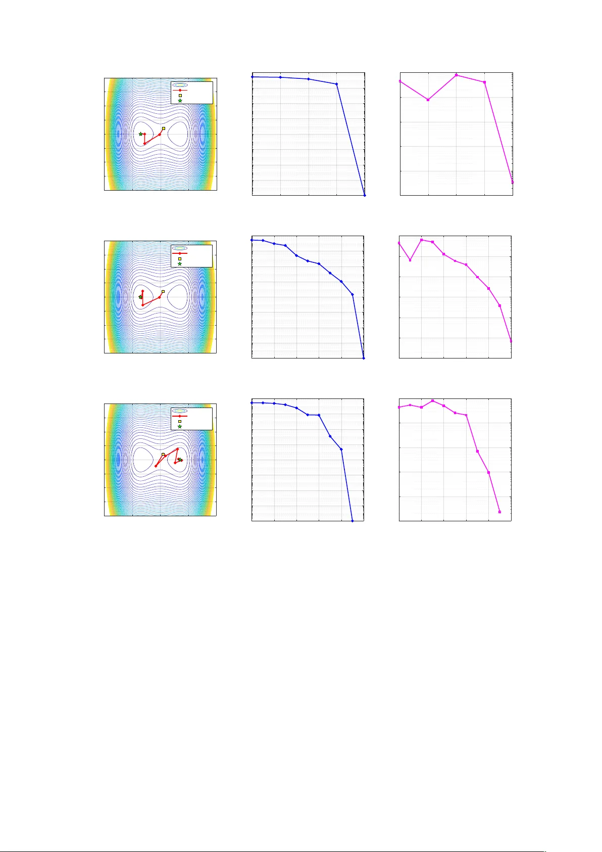
Y A U’S AFFINE NORMAL DESCENT: ALGORITHMIC FRAMEW ORK AND CONVER GENCE ANAL YSIS YI-SHUAI NIU 1 , AR T AN SHESHMANI 1 , 3 , AND SHING-TUNG Y A U 1 , 2 Abstract. W e prop ose Y au’s Aﬃne Normal Descen t (Y AND), a geometric framework for smo oth unconstrained optimization in whic h searc h directions are deﬁned b y the equi–aﬃne normal of lev el-set hypersurfaces. The resulting directions are in v arian t under v olume- preserving aﬃne transformations and in trinsically adapt to anisotropic curv ature. Using the analytic represen tation of the aﬃne normal from aﬃne diﬀerential geometry , we estab- lish its equiv alence with the classical slice–cen troid construction under con v exit y . F or strictly con vex quadratic ob jectives, aﬃne-normal directions are collinear with Newton directions, implying one-step con v ergence under exact line searc h. F or general smooth (possibly noncon- v ex) ob jectives, w e characterize precisely when aﬃne-normal directions yield strict descent and dev elop a line-searc h-based Y AND. W e establish global conv ergence under standard smo othness assumptions, linear conv ergence under strong conv exity and Poly ak– Lo jasiewicz conditions, and quadratic local conv ergence near nondegenerate minimizers. W e further sho w that aﬃne-normal directions are robust under aﬃne scalings, remaining insensitive to arbitrarily ill-conditioned transformations. Numerical exp erimen ts illustrate the geometric b eha vior of the metho d and its robustness under strong anisotropic scaling. Contents 1. In tro duction 2 2. Aﬃne normal direction 5 2.1. Tw o form ulas for the aﬃne normal direction 5 2.2. Equiv alence of the analytical and slice-centroid formulas under con v exit y 7 2.3. Role of conv exit y 9 2.4. Geometric illustration 10 2.5. Computational complexity 10 3. Equiv alence of aﬃne normal and Newton directions for strictly con v ex quadratics 10 4. When is the aﬃne normal a descen t direction? 12 4.1. Strict descent holds exactly at elliptic p oin ts 12 4.2. Momen t-based constructions require con v exit y 13 5. Examples for computing the aﬃne normal 13 5.1. Quadratic conv ex function in t w o V ariables 13 5.2. Quadratic conv ex function in three v ariables 14 5.3. Strictly conv ex non-quadratic example 15 6. Y AND 15 6.1. Aﬃne normal descent direction 15 6.2. Y AND algorithm 16 7. Con v ergence analysis of Y AND 17 7.1. Preliminaries 18 7.2. Strongly conv ex and smo oth case: Armijo backtrac king 21 7.3. Noncon v ex setting: global linear conv ergence with PL inequality 22 7.4. Noncon v ex setting: strong W olfe and gradient con vergence 23 2020 Mathematics Subje ct Classiﬁc ation. 90C15, 90C30, 49M37, 53A15. Key wor ds and phr ases. Y au’s aﬃne normal descent, aﬃne diﬀerential geometry , aﬃne inv ariance, nonlin- ear optimization, global con vergence, lo cal quadratic con vergence. 1 2 YI-SHUAI NIU 1 , AR T AN SHESHMANI 1 , 3 , AND SHING-TUNG Y AU 1 , 2 7.5. Exact line search: factor–tw o improv emen t 24 7.6. Lo cal quadratic con v ergence 26 7.7. Summary of conv ergence regimes 29 8. Bey ond quadratic rates?—lo cal order vs global geometry 29 9. Aﬃne-scaling mo dels and condition-num b er robustness 30 9.1. Aﬃne-scaling mo del 31 9.2. Three basic in v ariances: unimodular cov ariance, isotropic scaling, and step-size absorption 31 9.3. Exact inv ariance under general aﬃne scaling 33 9.4. Extension to Armijo line search 34 9.5. Extension to strong W olfe line search 35 9.6. Uniﬁed aﬃne inv ariance of monotone line-search rules 36 9.7. Regime-wise transfer and explicit rates 36 9.8. Illustrativ e examples 37 10. Numerical exp eriments 38 10.1. Exp erimen tal setup 38 10.2. Con v ex quadratic problems 39 10.3. Smo oth nonquadratic con v ex problems 42 10.4. Smo oth nonconv ex problems 45 10.5. Summary of numerical results 48 11. Conclusion 48 Ac kno wledgements 51 App endix A. The aﬃne normal 51 A.1. F oundational concepts 51 A.2. Gauss formula and induced structures 52 A.3. V olume forms and equi–aﬃne theory 52 A.4. Existence and uniqueness 53 A.5. Lo cal co ordinate expressions 53 A.6. T ransformation prop erties 54 A.7. Sp ecial cases and examples 54 A.8. Generalizations and extensions 54 References 55 Author Information 55 1. Intr oduction Designing optimization algorithms that are robust to scaling, conditioning, and co ordinate transformations remains a cen tral c hallenge in mathematical programming. A fundamental diﬃcult y lies in the mismatch b et ween the geometry of the ob jectiv e function and the geom- etry implicitly imp osed b y the algorithm. Classical metho ds such as gradien t descen t and Newton’s metho d rely on Euclidean or lo cally quadratic mo dels, whose p erformance can de- grade sev erely under aﬃne transformations of the v ariables. Ev en for simple conv ex problems, aﬃne scalings can arbitrarily disto rt the geometry of lev el sets, leading to ill-conditioning and p oor algorithmic behavior. A recurring geometric principle is that optimization p erformance is gov erned by the shap e of level sets. Gradien t descen t p erforms well when lev el sets are nearly spherical, while Newton’s metho d is exact for strictly conv ex quadratic functions with ellipsoidal lev el sets. Ho w ever, these metho ds do not deriv e their searc h directions from the intrinsic geometry of lev el sets themselves. This raises a fundamental question: Y AU’S AFFINE NORMAL DESCENT 3 Can one design optimization metho ds whose se ar ch dir e ctions ar e determine d dir e ctly by the intrinsic ge ometry of level sets, and ar e ther efor e inher ently aﬃne invariant? Aﬃne inv ariance is widely regarded as a desirable structural prop erty for mitigating sen- sitivit y to scaling and reparameterization. Existing approac hes achiev e in v ariance b y pre- scribing a geometry on the am bien t space, such as through barrier functions, norm-based structures, or Mink o wski gauges [ 12 , 11 , 6 , 7 ]. In con trast, w e derive in v ariance directly from the intrinsic geometry of lev el sets, without relying on an y externally prescrib ed metric. Sp eciﬁcally , w e consider the smooth unconstrained problem min x ∈ R n +1 f ( x ) , where f is suﬃciently smo oth. At a current iterate x k , we examine the lev el-set hypersurface L k := { x : f ( x ) = f ( x k ) } , and extract a searc h direction from its equi–aﬃne geometry . The geometric ob ject underlying our construction is the aﬃne normal , a classical notion in aﬃne diﬀerential geometry , deﬁned as a canonical transversal direction determined solely b y the lo cal shap e of a hypersurface, indep enden t of parametrization, and in v arian t under unimo dular (v olume-preserving) aﬃne transformations. Unlik e the Euclidean normal (the gradien t), the aﬃne normal enco des higher-order geometric information in a co ordinate- free manner. F or quadratic functions with ellipsoidal lev el sets, the aﬃne normal at ev ery p oin t p oin ts directly to ward the unique critical p oint. Consequently , aﬃne normal directions coincide with Newton directions in the quadratic case, although the aﬃne normal itself is deﬁned indep enden tly of second-order T a ylor expansions. This geometric exactness motiv ates its use as a descent direction b ey ond quadratic mo dels. The use of aﬃne-normal geometry for optimization was initiated b y Cheng–Cheng–Y au [ 5 ], who prop osed deriving searc h directions from equi–aﬃne normal directions of lev el sets. This w ork reveals a fundamental geometric principle: optimization directions can be deﬁned intrin- sically from lev el-set geometry , rather than from lo cal T a ylor expansions. F or conv enience, w e refer to metho ds that follow this principle as Y au-typ e (or Y au-like ) metho ds. T o date, ho w ever, no general algorithmic framew ork or conv ergence theory based on this principle has b een established. W e dev elop a complete optimization framew ork based on aﬃne-normal geometry . W e in tro duce the Y au’s aﬃne normal desc ent (Y AND) algorithm for smo oth unconstrained op- timization and establish its fundamental algorithmic prop erties. Our analysis sho ws that the aﬃne-normal direction provides a curv ature-a w are search direction derived from the intrinsic geometry of lev el sets, leading to strong inv ariance prop erties and fa v orable local conv ergence b eha vior. A t eac h iteration, the search direction is giv en by the aﬃne normal to the current level set, follow ed by a line searc h. Since the aﬃne normal is deﬁned only up to scale, step sizes are determined indep endently using standard rules (e.g., exact line search, Armijo, or strong W olfe conditions). By construction, the resulting direction is in v ariant under unimo dular aﬃne transformations of v ariables. Conceptually , Y AND pro vides a geometric in terpretation of curv ature-a w are optimization directions that dep end only on the in trinsic structure of lev el sets rather than on a particular coordinate represen tation. A cen tral subtlety is that the aﬃne normal is not automatically a descen t direction. W e sho w that strict descen t holds precisely at el liptic p oints , where the Hessian restricted to the tangen t space of the level set is p ositiv e deﬁnite. A t non-elliptic p oin ts, the aﬃne normal ma y fail to p oin t inw ard, which necessitates a computable ellipticit y test and a principled orien tation correction. This yields a w ell-deﬁned algorithm applicable to general smo oth (p ossibly nonconv ex) ob jectiv es. 4 YI-SHUAI NIU 1 , AR T AN SHESHMANI 1 , 3 , AND SHING-TUNG Y AU 1 , 2 W e establish global and lo cal con v ergence guarantees for Y AND. Globally , under standard smo othness assumptions and appropriate line-search rules, the metho d admits conv ergence guaran tees comparable to ﬁrst-order metho ds; in particular, we obtain linear conv ergence under strong conv exit y and P olyak– Lo jasiewicz conditions, and gradient conv ergence under strong W olfe conditions for general noncon v ex ob jectives. Lo cally , near a nondegenerate minimizer, the aﬃne normal direction coincides with the Newton direction up to second- order terms, which implies lo cal quadratic con v ergence under standard assumptions. This relationship provides a geometric interpretation of Newton’s metho d: in the quadratic case the aﬃne normal exactly reco vers the Newton direction, while b ey ond the quadratic setting it yields a curv ature-aw are search direction deriv ed directly from level-set geometry . Imp or- tan tly , aﬃne-normal directions are deﬁned intrinsically from level-set geometry and do not rely on explicit Hessian inv ersion or quadratic models. Th us, Y AND combines robust global b eha vior with high local eﬃciency , while being in trinsically equi–aﬃne inv arian t. In addition, we study the behavior of aﬃne-normal directions under aﬃne-scaled qua- dratic mo dels and sho w that the resulting search directions are unaﬀected b y arbitrarily ill-conditioned linear scalings. This provides a geometric explanation of the robustness of aﬃne-normal descent with resp ect to anisotropic aﬃne transformations. The main contributions of this pap er are as follo ws: • W e establish the Y AND framew ork, which deﬁnes optimization directions intrinsically from the equi–aﬃne geometry of lev el sets. • W e characterize precisely when aﬃne-normal directions yield strict descen t, leading to a well-deﬁned algorithm for general smo oth (p ossibly nonconv ex) ob jectiv es. • W e establish global con v ergence under standard line-searc h rules, linear conv ergence under strong con v exit y and P oly ak– Lo jasiewicz conditions, and quadratic local con- v ergence near nondegenerate minimizers. • W e pro v e that aﬃne-normal directions are inherently robust under arbitrarily ill- conditioned aﬃne scalings. Finally , we presen t a series of numerical experiments that illustrate the geometric b eha vior of the proposed metho d. Rather than performing large-scale b enc hmarking, the exp eri- men ts are designed to highligh t c haracteristic phenomena, including robustness under aﬃne scalings, behavior on ill-conditioned quadratic mo dels, and represen tative con v ex/nonconv ex test problems. Comparisons with classical metho ds such as gradient descent and Newton’s metho d further illustrate the distinct conv ergence b eha vior of aﬃne-normal descen t predicted b y the theory . Large-scale implemen tation and b enc hmarking are deferred to future w ork. T able 1 p ositions Y AND relative to representativ e geometry-aw are optimization paradigms, highligh ting the geometric ob ject deﬁning each direction, the required information, and k ey structural prop erties. The remainder of the pap er is organized as follows. Section 2 reviews the aﬃne normal construction and its analytic represen tation for level sets. Section 3 establishes the corre- sp ondence b et ween aﬃne normal directions and Newton steps for strictly conv ex quadratic ob jectives. Section 4 c haracterizes descen t and ellipticit y conditions. Section 5 pro vides illus- trativ e examples for computing the aﬃne normal. Section 6 introduces the Y AND algorithm together with line-searc h strategies. Section 7 establishes global and lo cal con v ergence re- sults. Section 8 discusses the p oten tial for beyond-quadratic conv ergence rates, highlighting the in terpla y b et w een lo cal order and global geometry . Section 9 analyzes aﬃne-scaling mo d- els and explains the robustness of aﬃne-normal directions with respect to condition n um b ers. Numerical exp eriments are reported in Section 10 , follo w ed b y concluding remarks. Y AU’S AFFINE NORMAL DESCENT 5 T able 1. High-level comparison of Y AND with represen tativ e geometric op- timization paradigms. Conv ergence rates refer to standard theoretical regimes (e.g., strong conv exit y , PL condition, or lo cal analysis). Metho d Direction-deﬁning ob ject Information needed T ypical guarantee Aﬃne inv ariance Typical limitation Newton / damp ed Newton Lo cal quadratic mo del via ∇ 2 f ( x ) Gradien t + Hessian solv e Quadratic lo cal con vergence; linear global with damping Linear aﬃne in v arian t Requires SPD (or regularization); unstable far from minimizers Quasi– Newton (BF GS/L- BF GS) Secan t-based metric appro ximation Gradien ts; curv ature pairs Sup erlinear lo cal con vergence (BF GS); linear global under standard assumptions Not aﬃne in v arian t Sensitiv e to scaling Natural gradien t [ 2 ] / Riemannian metho ds [ 1 ] Riemannian metric (e.g., Fisher information) Gradien t + metric (or in verse) T ypically linear con vergence Co ordinate in v arian t (metric- dep enden t) Requires problem-sp eciﬁc metric; curv ature assumptions Mirror descen t [ 4 ] Bregman div ergence (mirror map) Gradien t; pro x/mirror step O (1 /k ) for conv ex problems; O (1 /k 2 ) with acceleration Not aﬃne in v arian t P erformance dep ends on mirror c hoice In terior-p oin t (self- concordan t) Barrier geometry (Dikin ellipsoids) Barrier + deriv ativ es; Newton steps P olynomial-time global complexit y; quadratic lo cal con vergence Aﬃne in v arian t under barrier geometry Restricted to structured con vex problems Y AND Equi-aﬃne normal of lev el sets First/second deriv ativ es or momen t appro ximation Linear under PL/strong con vexit y; quadratic lo cal con vergence; exact on strictly con vex quadratics Equi-aﬃne in v arian t (v olume- preserving maps) T rue aﬃne normal in ward only at elliptic p oin ts; correction needed otherwise 2. Affine normal direction The concept of the aﬃne normal emerged from aﬃne diﬀerential geometry in the early 20th cen tury through the work of Blasc hke, Berwald, and others; see, e.g., [ 14 , 10 ]. Unlike Euclidean geometry , which privileges orthogonal transformations, aﬃne geometry studies prop erties inv arian t under the larger group of volume-preserving aﬃne transformations. The aﬃne normal represents the natural “normal direction” from this aﬃne-in v arian t persp ective. 2.1. Tw o form ulas for the aﬃne normal direction. 2.1.1. Derivative formula (analytic al expr ession). Let f : R n +1 → R , and at a p oin t z , consider the level set h ypersurface M = { x : f ( x ) = f ( z ) } . Rotate the co ordinate system so that the last axis aligns with ∇ f ( z ) (the “normal-aligned coordinates”). Deﬁne f i = ∂ x i f , f ij = ∂ x i ∂ x j f , f pq r = ∂ x p ∂ x q ∂ x r f , and denote [ f ij ] = [ f ij ] − 1 as the inv erse of the tangen t-tangen t blo c k of the Hessian ( i, j, p, q , r ∈ { 1 , . . . , n } ). Then the aﬃne normal direction (up to scale) can b e written 6 YI-SHUAI NIU 1 , AR T AN SHESHMANI 1 , 3 , AND SHING-TUNG Y AU 1 , 2 as (cf. Cheng-Cheng-Y au [ 5 ]) d AN ( z ) ∝   f ij  − 1 n + 2 ∥∇ f ∥ f pq f pq i + f n +1 ,i  − 1   (2.1) This giv es the co ordinate comp onen ts in the “normal-aligned” system; the mean curv ature factor app earing in the full geometric deriv ation is ignored here since only the direction is relev ant. 2.1.2. Slic e-c entr o id formula (ge ometric appr oximation). A t a p oint z , consider the tangent plane P ( x ) = ∇ f ( z ) · ( x − z ) = 0 , and its parallel family P ( x ) = C . The sublevel set is Ω z := { x : f ( x ) ≤ f ( z ) } . F or eac h C , deﬁne the slice S C := { x : P ( x ) = C } ∩ Ω z , and let g ( C ) be the cen troid of S C , when this region is a con v ex b o dy . Cho osing the normal so that C < 0 corresp onds to the in terior of Ω z , we deﬁne the slice-cen troid direction b y d SC ( z ) ∝ lim C ↑ 0 g ( C ) − z − C , if the limit exists. Numerically , for small δ > 0, b d SC ( z ) ∝ z − g ( − δ ) δ , whose truncation error is O ( δ ). This formula yields the analytic aﬃne normal (up to scale) precisely when z is an elliptic point 1 , i.e., when the slice S C is conv ex for C < 0 and shrinks smo othly to z . Outside the elliptic region (hyperb olic or parab olic p oin ts), the slices may b e noncon v ex or multi-component, and d SC ( z ) is no longer aligned with the analytic aﬃne normal. Note that this metho d requires only ﬁrst-order information (for constructing the tangen t plane) and a v oids third deriv atives and matrix inv ersion, though computing the high-dimensional centroid g ( C ) eﬃcien tly remains the main bottleneck. Remark 2.1 (Moment viewp oin t) . F rom the p ersp ectiv e of aﬃne integral geometry , the three constructions ab o v e ﬁt naturally into a hierarch y of geometric momen ts . The 0- th moment R K 1 dx records only the total mass (v olume) of a region K ; the ﬁrst moment R K x dx determines its cen troid; and the cen tered second moment R K ( x − G )( x − G ) ⊤ dx captures lo cal shap e via an inertia (ellipsoid) tensor. In this hierarch y , volume, centroid, and curv ature (enco ded b y the aﬃne metric and ultimately the aﬃne normal) corresp ond, resp ectiv ely , to 0-th, 1-st, and 2-nd order geometric momen ts. A t an elliptic p oin t of the lev el set, the analytic deriv ativ e formula, the slice-centroid construction, and the cap-cen troid construction all prob e the same second-order geometry . When expressed in a normal-aligned co ordinate chart and expanded to quadratic order, each construction recov ers the same aﬃne metric and therefore yields the same aﬃne normal direction. Th us the slice- and cap-based directions may b e in terpreted as in tegral (moment-based) realizations of the analytic aﬃne normal at elliptic p oin ts. In the next section, we make this precise by sho wing that, after appropriate normalization, b oth the slice and the cap directions con v erge in the limit to the analytic aﬃne normal, agreeing with it up to a p ositive scalar factor. 1 A p oint z is called elliptic if the tangent–tangen t Hessian at z is p ositive deﬁnite; in this case M is lo cally strictly conv ex. It is called hyperb olic if that blo c k is indeﬁnite, and parab olic if it is singular. Y AU’S AFFINE NORMAL DESCENT 7 2.2. Equiv alence of the analytical and slice-centroid formulas under con v exit y . The slice-cen troid form ula captures the aﬃne normal direction only when the lev el hyper- surface is lo cally strictly conv ex. In general nonconv ex situations, tangential drift ma y o ccur and the slice-cen troid direction may fail to agree with the analytical aﬃne-normal direction; see Subsection 1.3 for discussion. Theorem 2.2 (Consistency of slice-centroid and analytical aﬃne normal under conv exit y) . L et M = { x : f ( x ) = f ( z ) } b e the level hyp ersurfac e at z , and assume that M is lo c al ly strictly c onvex at z (e quivalently, the tangent-tangent Hessian of f is p ositive deﬁnite at z ). L et g ( C ) b e the c entr oid of the slic e S C = { x : P ( x ) = C } ∩ Ω z , Ω z = { f ≤ f ( z ) } , wher e P ( x ) = ∇ f ( z ) · ( x − z ) and C < 0 c orr esp onds to the interior. Then the inwar d one-side d limit lim C ↑ 0 z − g ( C ) − C exists and agr e es with the analytic al aﬃne-normal dir e ction at z , up to a p ositive sc alar multiple. Pr o of. Step 0 (Setup and c hoice of co ordinates) . By an equi-v olume aﬃne c hange of v ariables, translate z to the origin, align the tangen t plane with { t = 0 } , and align the normal ν = ∇ f ( z ) / ∥∇ f ( z ) ∥ with e n +1 . Denote the lo cal coordinates by ( u, t ) ∈ R n × R . Step 1 (Lo cal graph of the h yp ersurface) . In these co ordinates, after a further linear transformation that diagonalizes the second fundamen tal form, the hypersurface M has the expansion t = Φ( u ) = 1 2 | u | 2 + 1 6 C ij k u i u j u k + O ( | u | 4 ) , u ∈ R n , where ( C ij k ) is the totally symmetric Pic k cubic form, satisfying the ap olar (trace-free) con- dition n X j =1 C ij j = 0 , i = 1 , . . . , n. The absence of linear terms follo ws from the tangen t plane condition, and the quadratic term is normalized to 1 2 | u | 2 b y the choice of co ordinates that diagonalizes the second fundamental form. Under this equi-volume aﬃne normalization, the analytical aﬃne-normal direction at z is the + t direction. Step 2 (Sublev el set and slices) . The lo cal “interior” sublevel set is Ω z = { ( u, t ) : t ≥ Φ( u ) } . T ake the parallel slice planes P C = { ( u, t ) : t = C } with small C > 0. Then S C = { ( u, C ) : Φ( u ) ≤ C } is a b ounded conv ex set in R n . Denote its centroid by g ( C ) = ( ¯ u ( C ) , C ) , ¯ u ( C ) = 1 V ( C ) Z { Φ( u ) ≤ C } u du, V ( C ) = Z { Φ( u ) ≤ C } 1 du. Step 3 (Scaling) . Let u = √ C y to obtain Φ( √ C y ) = 1 2 C | y | 2 + 1 6 C 3 / 2 C ij k y i y j y k + O ( C 2 ) . Set ε = √ C and deﬁne D ε = n y : 1 2 | y | 2 + 1 6 ε C ( y , y , y ) + O ( ε 2 ) ≤ 1 o , B = { y : 1 2 | y | 2 ≤ 1 } . 8 YI-SHUAI NIU 1 , AR T AN SHESHMANI 1 , 3 , AND SHING-TUNG Y AU 1 , 2 Then V ( C ) = C n/ 2 | D ε | , Z { Φ( u ) ≤ C } u du = C ( n +1) / 2 Z D ε y dy , so ¯ u ( C ) = √ C R D ε y dy | D ε | . Step 4 (Boundary p erturbation and Hadamard v ariation) . W rite the b oundary as y = ρ ( θ ) θ , θ ∈ S n − 1 . F rom F ( ρ, ε ; θ ) = 1 2 ρ 2 + 1 6 ε ρ 3 C ( θ , θ , θ ) + O ( ε 2 ) − 1 = 0 , at ε = 0 we hav e ρ 0 = √ 2 and δ ρ ( θ ) := dρ dε     ε =0 = − ∂ F /∂ ε ∂ F /∂ ρ    ε =0 ,ρ = ρ 0 = − 1 3 C ( θ , θ , θ ) . By a Hadamard-type v ariation form ula, d dε    ε =0 Z D ε ψ ( y ) dy = Z ∂ B ψ ( y ) δ ρ ( θ ) dσ ( θ ) , y = ρ 0 θ . Step 5 (Apply to ψ ( y ) = y i ) . With ψ ( y ) = y i , d dε    ε =0 Z D ε y i dy = Z ∂ B y i δ ρ ( θ ) dσ ( θ ) = − 1 3 Z S n − 1 θ i C ( θ , θ , θ ) dσ ( θ ) . Using the spherical momen t identit y from Lemma 3: Z S n − 1 θ i θ a θ b θ c dσ ( θ ) = α n ( δ ia δ bc + δ ib δ ac + δ ic δ ab ) , where α n = σ n − 1 n ( n +2) and σ n − 1 denotes the surface area of S n − 1 , we compute: Z S n − 1 θ i C ( θ , θ , θ ) dσ ( θ ) = Z S n − 1 θ i θ a θ b θ c C abc dσ ( θ ) = α n C abc ( δ ia δ bc + δ ib δ ac + δ ic δ ab ) . This simpliﬁes to: α n ( C ibb + C ibi + C iib ) = 3 α n C ibb = 0 , b y the ap olar condition P b C ibb = 0. Therefore, Z D ε y dy = O ( ε 2 ) , and | D ε | = | B | + O ( ε 2 ) . Step 6 (Cen troid asymptotics and direction) . Therefore ¯ u ( C ) = √ C O ( ε 2 ) | B | + O ( ε 2 ) = O ( C 3 / 2 ) , and hence g ( C ) = ( O ( C 3 / 2 ) , C ) . Th us lim C ↓ 0 z − g ( C ) − C = (0 , . . . , 0 , 1) ∈ R n +1 . Step 7 (Recov ering the aﬃne normal) . Under the equi-v olume aﬃne normalization, (0 , . . . , 0 , 1) is the analytical aﬃne-normal direction. Undoing the normalization preserv es direction up to scale. □ The following Lemma is used in Step 5 to compute the ﬁrst v ariation of the cen troid. Y AU’S AFFINE NORMAL DESCENT 9 Lemma 2.3 (F ourth-moment tensor on the sphere) . F or the unit spher e S n − 1 , the fourth- or der spheric al moment satisﬁes Z S n − 1 θ i θ a θ b θ c dσ ( θ ) = α n ( δ ia δ bc + δ ib δ ac + δ ic δ ab ) , wher e α n = σ n − 1 n ( n +2) and σ n − 1 denotes the surfac e me asur e of S n − 1 . This identity fol lows fr om O ( n ) -invarianc e and the standar d spheric al moment formulas; se e, for example, F ang and Zhang [ 8 , Chapter 2] . Comparison of the t w o form ulas. • Deriv ativ e form ula: + Pros: Exact and deterministic direction; for con v ex quadratic forms, third deriv a- tiv es v anish and the direction is parallel to the Newton direction, leading to one- step con v ergence under line searc h (see Theorem 4). Con v enien t when automatic diﬀeren tiation is av ailable. – Cons: Requires in v ersion of the tangen t-tangent Hessian ( O ( n 3 )) and ev aluation of third deriv ativ es; sensitiv e to noise or degenerate Hessians; direction degener- ates when Hessian is singular. • Slice-centroid form ula: + Pros: Only requires ﬁrst deriv ativ es; b ypasses third deriv ativ es and matrix in- v ersion; more robust under noise; practical alternative when higher deriv atives are unav ailable. – Cons: The main diﬃcult y lies in computing the centroid of S C , whic h is expensive in high dimensions and generally requires approximation via sampling, numerical in tegration, or minimal-v olume ellipsoid estimation; accuracy and con v ergence dep end on sampling quality . 2.3. Role of conv exit y. Con v exit y plays a fundamen tal role in the agreemen t of the t w o aﬃne-normal constructions and in ensuring that the aﬃne normal serv es as a descent direction for f . W e summarize these relationships b elo w. Equiv alence of the t w o constructions. The analytic aﬃne normal agrees (up to a p ositiv e scalar) with the slice-centroid construction precisely at elliptic p oin ts of the level set, i.e., p oin ts where the tangen t-tangen t Hessian is p ositiv e deﬁnite and the lev el set is lo cally strictly conv ex. At suc h p oin ts, small slices are conv ex b o dies, their moments are well deﬁned, and the cen troid tra jectories repro duce the analytic aﬃne normal in the limit. Thus the equiv alence of the deriv ativ e formula and slice formula holds exactly on elliptic patches of the hypersurface. F ailure at non-elliptic p oin ts. A t h yp erbolic p oin ts, the tangen t-tangen t Hessian is indeﬁnite: the level set b ends in opposite directions, slices b ecome noncon v ex or m ulti- comp onen t, and their cen troids no longer reﬂect the analytic aﬃne normal. At parab olic p oin ts, the tangent-tangen t Hessian is singular and the aﬃne metric degenerates, so neither the analytic aﬃne normal nor the moment-based construction yield a meaningful normal direction. The counterexample in Example 4.3 illustrates that the slice-centroid direction ma y ev en b ecome an ascent direction in the noncon v ex case. Implications for descen t directions in optimization. The analytic aﬃne normal re- mains formally well deﬁned at an y nondegenerate p oint of the h yp ersurface, but it represents an in w ard geometric direction only at elliptic p oin ts. Consequently , the aﬃne normal is a guaran teed strict descent direction for f if eac h iterate x k lies on a lo cally strictly con v ex patc h of the lev el set. Within such a neigh b orho od, the in terior sublev el set { f ≤ f ( x k ) } lies on the inw ard side of the h yp ersurface, and the aﬃne normal p oints strictly in to this 10 YI-SHUAI NIU 1 , AR T AN SHESHMANI 1 , 3 , AND SHING-TUNG Y AU 1 , 2 region. Moreo v er, in the same elliptic neighborho o d, the slice-centroid and cap-cen troid con- structions provide consistent appro ximations of the analytic aﬃne normal, since all three directions coincide up to scaling. 2.4. Geometric illustration. T o close this section, w e include a simple tw o-dimensional picture (Figure 1) that visualizes the diﬀerence b etw een the Euclidean normal and the aﬃne normal deﬁned b y the slice-cen troid formula. On a con v ex curv e (an ellipse is sho wn), at a p oin t p , the Euclidean normal (red arro w) is giv en b y the gradient ∇ f ( p ), usually p oin ting out w ard, whereas the aﬃne normal (blue arrow) can b e obtained via the slice-centroid construction: shifting the tangent line in w ard and taking the cen troid of the chord segmen t inside the ellipse. As C → 0, the tangen t direction of the centroid tra jectory at p giv es the aﬃne normal direction. F or ellipses (aﬃne spheres), the aﬃne normals alw ays p oin t tow ard the center, sho wing the geometric distinction–Euclidean normal reﬂects lo cal orthogonalit y , while aﬃne normal enco des the global centroidal trend rather than merely lo cal orthogonality . cen ter p tangen t c hord cen troid Euclidean normal (gradient) Aﬃne normal (inw ard) Figure 1. Geometric comparison betw een the Euclidean and aﬃne normals 2.5. Computational complexity. The analytic expression of the aﬃne-normal direction in v olves ﬁrst-, second-, and third-order deriv atives of the ob jective function. In particular, ev aluating the analytic form ula requires computing deriv ativ es of the Hessian, whic h ma y b e computationally exp ensive in high-dimensional settings. In the presen t work our primary fo cus is on the geometric structure and conv ergence prop erties of aﬃne-normal descent. The developmen t of eﬃcient tec hniques for computing or appro ximating the aﬃne-normal direction in large-scale problems is an imp ortan t topic for future research. 3. Equiv alence of affine normal and Newton directions for strictl y convex quadra tics Theorem 3.1 (Aﬃne normal coincides with the Newton direction on strictly conv ex quadrat- ics) . L et f : R n +1 → R b e a strictly c onvex quadr atic f ( x ) = 1 2 x ⊤ Ax + b ⊤ x + c, A ≻ 0 . F or any x with ∇ f ( x )  = 0 , the aﬃne normal dir e ction d AN ( x ) of the level set { y : f ( y ) = f ( x ) } is c ol line ar with the Newton dir e ction d N ( x ) = − ( ∇ 2 f ( x )) − 1 ∇ f ( x ) = − A − 1 ∇ f ( x ) , that is, ther e exists λ ( x ) > 0 such that d AN ( x ) = λ ( x ) d N ( x ) . When ∇ f ( x ) = 0 , b oth vanish, trivial ly satisfying the claim. Y AU’S AFFINE NORMAL DESCENT 11 Pro of 1 (Geometric Argumen t). When A ≻ 0, the lev el sets of f are concen tric ellipsoids cen tered at x ⋆ = − A − 1 b . By aﬃne diﬀeren tial geometry , the aﬃne normals of an ellipsoid p oin t to w ard its cen ter. Hence for any x  = x ⋆ , the aﬃne normal direction is along x ⋆ − x . Mean while, d N ( x ) = − A − 1 ∇ f ( x ) = − A − 1 ( Ax + b ) = x ⋆ − x, hence they are parallel. □ Pro of 2 (Analytical Argumen t via Blo c k Matrix and Sc h ur Complement). Step 1 (Change of basis and notation). At x , choose an orthonormal basis so that the last axis e n +1 is parallel to ∇ f ( x ) and the ﬁrst n axes are tangent to the level set. W rite the Hessian ∇ 2 f ( x ) = A in blo ck form A =  B c c ⊤ d  , where B ∈ R n × n (the tangen t–tangen t blo ck [ f ij ]), c ∈ R n (the mixed normal–tangent blo c k [ f n +1 ,i ]), and d = f n +1 ,n +1 . Step 2 (Explicit aﬃne-normal direction in this basis). In the normal-aligned co ordi- nates, the aﬃne normal reads d AN ( x ) ∝  f ij  − 1 n +2 |∇ f | f pq f pq i + f n +1 ,i  − 1  , where [ f ij ] = [ f ij ] − 1 is the inv erse of the tangen t–tangen t blo c k. F or a quadratic form, all third deriv ativ es v anish, hence f pq i ≡ 0, and we get d AN ( x ) ∝  B − 1 c − 1  . Step 3 (Parallelism with the Newton direction). In the same basis, ∇ f = ∥∇ f ∥ e n +1 . Therefore d N ( x ) = − A − 1 ∇ f ( x ) = −∥∇ f ( x ) ∥ ·  last column of A − 1  . Let S := d − c ⊤ B − 1 c > 0 be the Sc h ur complement (since A ≻ 0). Then A − 1 =  B − 1 + B − 1 c S − 1 c ⊤ B − 1 − B − 1 c S − 1 − S − 1 c ⊤ B − 1 S − 1  , so the last column is  − B − 1 c S − 1 , S − 1  ⊤ . Hence d N ( x ) = ∥∇ f ( x ) ∥ S − 1  B − 1 c − 1  , whic h sho ws d N ∥ d AN and they diﬀer only by the p ositiv e scalar ∥∇ f ∥ S − 1 . □ Corollary 3.2 (One-step conv ergence with exact line search) . L et f ( x ) = 1 2 x ⊤ Ax + b ⊤ x + c with A symmetric p ositive deﬁnite and minimizer x ⋆ = − A − 1 b . F or any x with ∇ f ( x )  = 0 , an exact line se ar ch along the aﬃne-normal dir e ction r e aches x ⋆ in one step. Pr o of. T ak e any x with ∇ f ( x )  = 0. By Theorem 3.1 , d AN ( x ) is collinear with d N ( x ). F or a quadratic, d N ( x ) = − ( ∇ 2 f ) − 1 ∇ f ( x ) = − A − 1 ( Ax + b ) = x ⋆ − x. Hence there exists a scalar λ ( x ) > 0 suc h that d AN ( x ) = λ ( x ) d N ( x ) = λ ( x )( x ⋆ − x ) . 12 YI-SHUAI NIU 1 , AR T AN SHESHMANI 1 , 3 , AND SHING-TUNG Y AU 1 , 2 Consider the univ ariate function ϕ ( α ) := f ( x + α d AN ( x )), Since f is quadratic, ∇ f ( x + αd AN ( x )) = Ax + b + αAd AN ( x ) , and thus ϕ ′ ( α ) = d AN ( x ) ⊤  Ax + b + α Ad AN ( x )  . Substituting d AN ( x ) = λ ( x )( x ⋆ − x ) and Ax + b = A ( x − x ⋆ ) gives ϕ ′ ( α ) = λ ( x )( x ⋆ − x ) ⊤  A ( x − x ⋆ ) + αλ ( x ) A ( x ⋆ − x )  = λ ( x ) 2 ∥ x ⋆ − x ∥ 2 A ( αλ ( x ) − 1) , where ∥ v ∥ 2 A = v ⊤ Av . Since ∥ x ⋆ − x ∥ 2 A > 0 and λ ( x ) > 0, the deriv ativ e ϕ ′ ( α ) v anishes if and only if α ∗ = 1 λ ( x ) , whic h is the unique minimizer of ϕ . The corresponding up date is x + = x + α ∗ d AN ( x ) = x + 1 λ ( x ) λ ( x )( x ⋆ − x ) = x ⋆ . If ∇ f ( x ) = 0, then x = x ⋆ and the statement holds trivially . □ This sho ws that, on strictly con v ex quadratic ob jectiv es, the aﬃne normal direction coin- cides with the Newton direction (up to a p ositive scalar m ultiple). In particular, with exact line search, the resulting one-step update reaches the minimizer. Hence, in the quadratic setting, Newton direction app ears as a sp ecial case of the aﬃne-normal direction framew ork. 4. When is the affine normal a descent direction? The aﬃne normal direction is alwa ys w ell-deﬁned when the tangen t–tangen t blo ck of the Hessian is in v ertible. Ho wev er, its desc ent prop ert y dep ends crucially on the lo cal conv exit y of the level set. In this section we c haracterize precisely when the aﬃne normal is a strict descen t direction, and explain why moment-based constructions (slice–cen troid and cap– cen troid) require conv exit y . 4.1. Strict descen t holds exactly at elliptic p oints. Theorem 4.1 (Strict descen t at elliptic p oin ts) . L et f ∈ C 3 and ∇ f ( z )  = 0 , and assume the tangent–tangent Hessian at z is invertible. Then the analytic aﬃne normal d AN ( z ) satisﬁes ⟨∇ f ( z ) , d AN ( z ) ⟩ < 0 ⇐ ⇒ z is el liptic . Pr o of. In a normal-aligned frame, the aﬃne normal has the form d AN ( z ) = λ ( z )  τ ( z ) − 1  , where τ is determined by the tangen t–tangen t Hessian and λ ( z ) =  det h ij ( z )  − 1 / ( n +2) is the aﬃne normalization factor. The sign of λ ( z ) is determined b y the sign of det( h ij ). If z is elliptic, then h ij is p ositiv e deﬁnite and det h ij > 0, hence λ ( z ) > 0. Since ∇ f ( z ) = ∥∇ f ( z ) ∥ e n +1 , ⟨∇ f ( z ) , d AN ( z ) ⟩ = − λ ( z ) ∥∇ f ( z ) ∥ < 0 . If z is hyperb olic, then det( h ij ) < 0; no c hoice of λ ( z ) pro duces an inw ard-pointing real aﬃne normal. If z is parab olic, h ij is singular and the aﬃne normal is not deﬁned. □ Y AU’S AFFINE NORMAL DESCENT 13 Remark 4.2 (Geometric meaning) . Ellipticit y means that the lev el set is lo cally strictly con v ex; in this case the aﬃne normal p oin ts strictly in to the in terior of the sublev el set and its normalization factor is p ositiv e. When the tangent–tangen t Hessian is indeﬁnite (h yp erb olic p oin ts), the lev el set is not lo cally con v ex, and nearb y slices may b ecome nonconv ex or m ulti- comp onen t. The aﬃne normal no longer represents an in w ard v ariational direction in this situation. At parab olic points the tangent–tangen t Hessian is singular and the aﬃne metric degenerates, so the aﬃne normal is not well deﬁned. 4.2. Momen t-based constructions require con v exit y. The analytic aﬃne normal exists without con v exity , but its moment-b ase d approximations require it. Indeed, the slice–cen troid form ulation assumes that the intersection of the lev el set with a nearb y plane is a conv ex b ody with a well-behav ed centroid tra jectory . This fails when the lev el set is noncon v ex. Example 4.3 (Slice-cen troid fails to b e a descen t direction in the noncon vex case) . Consider in R 2 the nonconv ex function f ( x, y ) = ( x 2 − 1) 2 + y − 1 , z = (0 , 0) , for which f ( z ) = 0 and ∇ f ( z ) = (0 , 1). The tangen t line at z is y = 0, and Ω z = { ( x, y ) : f ( x, y ) ≤ 0 } = { y ≤ 1 − ( x 2 − 1) 2 } is nonconv ex. F or C < 0, the slice S C = { ( x, C ) : ( x 2 − 1) 2 ≤ 1 − C } consists of t wo disconnected symmetric in terv als, hence its centroid is g ( C ) = (0 , C ). Th us the slice-centroid direction b d SC ( z ) ∝ g (0) − g ( − δ ) δ = (0 , 1) satisﬁes ⟨∇ f ( z ) , b d SC ( z ) ⟩ = 1 > 0 , an ascent direction. This reﬂects the non-ellipticity at z and shows that the slice-centroid construction require lo cal conv exit y . 5. Examples for computing the affine normal Although the aﬃne normal originates from aﬃne diﬀeren tial geometry , its computation can b e made completely explicit in standard optimization settings. T o facilitate understanding for readers in optimization, w e b egin with a few low–dimensional examples in which the aﬃne normal can b e computed analytically and directly compared with classical directions such as the gradient and the Newton. 5.1. Quadratic con v ex function in tw o V ariables. Let f ( x, y ) = 1 2 ( x 2 + 4 y 2 ) − x − 4 y , with A = diag(1 , 4) ≻ 0 , b = ( − 1 , − 4), minimizing at x ⋆ = (1 , 1). Pick p = (2 , 0). Gradien t and Hessian. ∇ f ( x, y ) = ( x − 1 , 4 y − 4) , ∇ f ( p ) = (1 , − 4) , H = ∇ 2 f = A =  1 0 0 4  . Unit normal/tangen t ( n = 1 ). ∥∇ f ( p ) ∥ = √ 17 , ˆ n = ∇ f ( p ) ∥∇ f ( p ) ∥ =  1 √ 17 , − 4 √ 17  , ˆ t =  4 √ 17 , 1 √ 17  . 14 YI-SHUAI NIU 1 , AR T AN SHESHMANI 1 , 3 , AND SHING-TUNG Y AU 1 , 2 Recall ( n = 1 ). In the orthonormal frame ( ˆ t , ˆ n ), d AN ∝ ( τ , − 1) , τ = f 21 f 11 − ∥∇ f ∥ 3 f 111 f 2 11 with f 11 = D 2 f [ ˆ t , ˆ t ] , f 21 = D 2 f [ ˆ n , ˆ t ] , f 111 = D 3 f [ ˆ t , ˆ t , ˆ t ] . Directional deriv ativ es (quadratic case). Here f 111 = 0, so τ = f 21 /f 11 with f 11 = ˆ t ⊤ H ˆ t = 20 17 , f 21 = ˆ n ⊤ H ˆ t = − 12 17 , τ = − 3 5 . Aﬃne-normal direction. d AN ∝ τ ˆ t − ˆ n = 1 √ 17 ( − 3 . 4 , 3 . 4) ∥ ( − 1 , 1) . Newton direction. d N = − H − 1 ∇ f ( p ) = ( − 1 , 1) . Th us d AN ∥ d N . 5.2. Quadratic con v ex function in three v ariables. Let f ( x, y , z ) = 1 2 ( x 2 + 4 y 2 + 9 z 2 ) + ( − 1 , 0 , 0) · ( x, y , z ) , so A = diag(1 , 4 , 9) ≻ 0 , b = ( − 1 , 0 , 0) and x ⋆ = (1 , 0 , 0). T ak e p = (2 , 0 , 0). Gradien t and Hessian. ∇ f ( x, y , z ) = ( x − 1 , 4 y , 9 z ) , ∇ f ( p ) = (1 , 0 , 0) , H = diag(1 , 4 , 9) . Normal alignmen t and tangen ts ( n = 2 ). ˆ n = (1 , 0 , 0) , ˆ t 1 = (0 , 1 , 0) , ˆ t 2 = (0 , 0 , 1) . Blo c ks. B = diag(4 , 9) , c = (0 , 0) . Aﬃne-normal direction ( n = 2 ). F or quadratics (no third deriv ativ es), d AN ∝ 2 X i =1 ( B − 1 c ) i ˆ t i − ˆ n = − ˆ n = ( − 1 , 0 , 0) . Newton direction. d N = − H − 1 ∇ f ( p ) = ( − 1 , 0 , 0) . Th us d AN ∥ d N . Y AU’S AFFINE NORMAL DESCENT 15 5.3. Strictly con v ex non-quadratic example. Consider n = 1 and f ( x, y ) = 1 2 x 2 + 2 y 2 + 1 12 x 4 . Then ∇ 2 f ( x, y ) =  1 + x 2 0 0 4  ≻ 0 , so f is strictly conv ex. A t p = (1 , 1), in the orthonormal frame ( ˆ t , ˆ n ) the aﬃne normal direction is d AN ∝ ( τ , − 1) , τ = f 21 f 11 − ∥∇ f ∥ 3 f 111 f 2 11 with the ingredients computed in the text; numerically one ﬁnds τ ≈ 0 . 7687 and d AN ∝ ( − 1 . 0454 , − 0 . 7056) , ∇ f (1 , 1) · d AN ≈ − 4 . 2164 < 0 , conﬁrming strict descent. 6. Y AND W e no w transition from the geometric theory of aﬃne normals to the optimization al- gorithm that uses these directions as search directions. Since the analytic aﬃne normal is deﬁned only up to a nonzero scalar (and in particular, up to sign), w e m ust ensure that the c hosen direction is alw a ys a descent direction for f . 6.1. Aﬃne normal descen t direction. Given an iterate x k with ∇ f ( x k )  = 0, w e ﬁrst compute the aﬃne normal d AN ( x k ) of the level set { f = f ( x k ) } and deﬁne the searc h direction b y d k :=        d AN ( x k ) , if ⟨∇ f ( x k ) , d AN ( x k ) ⟩ < 0 , − d AN ( x k ) , if ⟨∇ f ( x k ) , d AN ( x k ) ⟩ > 0 , −∇ f ( x k ) / ∥∇ f ( x k ) ∥ , otherwise . (6.1) The third case corresp onds to an aﬃne-degenerate p oin t where the equi–aﬃne curv ature v anishes and the aﬃne normal collapses in to the tangen t space. At suc h p oin ts, an y vector v tan in the tangen t space satisﬁes ⟨∇ f ( x k ) , v tan ⟩ = 0, so the aﬃne normal (even if formally computable) cannot serve as a descen t direction. Since no representativ e with a negativ e normal comp onen t exists, we fall bac k to the steepest–descent direction −∇ f ( x k ) / ∥∇ f ( x k ) ∥ . The sign correction ensures ⟨∇ f ( x k ) , d k ⟩ < 0 , so d k is alwa ys a strict descen t direction of f at x k . T o analyze the geometry of d k , we work in the normal–aligne d fr ame at x k . Let e n +1 := ∇ f ( x k ) ∥∇ f ( x k ) ∥ , where { e i } n i =1 is an orthonormal basis for the tangen t space of the level set { f = f ( x k ) } . In this frame, every descen t direction d k constructed from ( 6.1 ) can b e expressed as d k = n X i =1 ( τ k ) i e i − e n +1 , τ k ∈ R n , as illustrated in Figure 2 . Let T k := ∥ τ k ∥ . Then ∥ d k ∥ 2 = 1 + T 2 k , so the scalar T k measures the tangen tial magnitude of the aﬃne–normal direction. Its bound- edness plays a cen tral role in the conv ergence analysis dev elop ed in Section 7 . 16 YI-SHUAI NIU 1 , AR T AN SHESHMANI 1 , 3 , AND SHING-TUNG Y AU 1 , 2 e i e n +1 { f = f ( x k ) } x k ∇ f ( x k ) d k = d AN ( x k ) ( τ k ) i − 1 Case 1: ⟨∇ f ( x k ) , d AN ( x k ) ⟩ < 0 e i e n +1 { f = f ( x k ) } x k ∇ f ( x k ) d AN ( x k ) d k = − d AN ( x k ) ( τ k ) i − 1 Case 2: ⟨∇ f ( x k ) , d AN ( x k ) ⟩ > 0 e i e n +1 { f = f ( x k ) } x k ∇ f ( x k ) d k = −∇ f ( x k ) / ∥∇ f ( x k ) ∥ ( τ k ) i = 0 − 1 Case 3: ⟨∇ f ( x k ) , d AN ( x k ) ⟩ = 0 Figure 2. Normal–aligned frame at x k illustrating three typical construc- tions of d k . The analytic aﬃne normal d AN ( x k ) is represen ted in the frame { e 1 , . . . , e n , e n +1 } with its ( n + 1)-st comp onen t normalized to − 1. Case 1: the aﬃne normal is already a descent direction ( ⟨∇ f ( x k ) , d AN ( x k ) ⟩ < 0), hence d k = d AN ( x k ). Case 2: the aﬃne normal p oin ts uphill ( ⟨∇ f ( x k ) , d AN ( x k ) ⟩ > 0), so we ﬂip the sign and set d k = − d AN ( x k ). Case 3: the aﬃne normal is orthog- onal to the gradient ( ⟨∇ f ( x k ) , d AN ( x k ) ⟩ = 0); in this degenerate case w e revert to the steep est–descen t direction d k = −∇ f ( x k ) / ∥∇ f ( x k ) ∥ . Remark 6.1 (Wh y using the ne gative aﬃne–normal direction in Case 2) . The sign correction in ( 6.1 ) ensures descen t by ﬂipping the aﬃne normal direction when ⟨∇ f ( x k ) , d AN ( x k ) ⟩ > 0. This is not merely an algorithmic ﬁx, and rather is gov erned by a deeper geometric justiﬁcation. Roughly sp eaking, at non-elliptic points, the lev el set p ossesses saddle-like or degenerate geometry , which implies that while the analytical aﬃne normal ma y p oin t uphill, its construction p ersists to enco de the “v aluable” curv ature information. Sp eciﬁcally , the aﬃne normal direction d AN is deriv ed from the aﬃne metric and the cubic form, which together suppress con tributions from directions where the level set curv ature is extreme (whether positive or negativ e). Consequently , the negativ e direction − d AN is aligned with the axis along whic h the Monge-Amp ` ere measure of the lo cal sublev el set, go verned b y det( ∇ 2 f ), con tracts most sharply . This mak es − d AN a geometry-aw are descent direction that is often more stable and eﬀective than b oth the ra w negative gradien t (which ignores the curv ature) and the Newton direction (which can b e misled b y negative eigen v alues). Therefore, “ the sign ﬂip ”, lev erages the geometric strength of the aﬃne normal construction, even outside the elliptic regime. Note that the aﬃne normal is fundamentally linked to the Monge-Amp ` ere operator deﬁned b y the aﬃne metric. At a p oin t x , the Monge-Amp ` ere measure of the sublev el set { y : f ( y ) ≤ f ( x ) } , to second order, is prop ortional to det( ∇ 2 f ( x )). The aﬃne normal direction ξ is c haracterized b y the condition that the volume form ω ξ induced b y ξ is parallel with resp ect to the aﬃne connection. When ⟨∇ f , ξ ⟩ > 0, the vector − ξ points in the direction where this canonical v olume form con tracts most rapidly , i.e., the direction along which the lo cal sublev el-set volume decreases fastest, providing a geometrically intrinsic and stable descen t direction even in noncon v ex regions. 6.2. Y AND algorithm. W e no w summarize the prop osed Y AND algorithm as follo ws: (1) Initialize x 0 , tolerance ε > 0, and a step strategy (exact line search / strong W olfe / Armijo). (2) F or k = 0 , 1 , 2 , . . . : (a) If ∥∇ f ( x k ) ∥ ≤ ε , stop. (b) Compute the descen t direction d k at x k according to ( 6.1 ). (c) Line searc h: take α k > 0 satisfying one of • Exact: α k ∈ arg min α ≥ 0 f ( x k + α d k ). Y AU’S AFFINE NORMAL DESCENT 17 • Armijo [ 3 ] : f ( x k + α k d k ) ≤ f ( x k ) + σ α k ∇ f ( x k ) ⊤ d k , (0 < σ < 1) . • Strong W olfe [ 16 ] : ( f ( x k + α k d k ) ≤ f ( x k ) + c 1 α k ∇ f ( x k ) ⊤ d k , |∇ f ( x k + α k d k ) ⊤ d k | ≤ c 2 |∇ f ( x k ) ⊤ d k | (0 < c 1 < c 2 < 1) . (d) Up date x k +1 = x k + α k d k . Remark 6.2 (Gradient is still required) . Although the search direction d k is deﬁned by the aﬃne normal, the gradien t ∇ f ( x k ) remains essential: (i) the aﬃne normal construction requires the Euclidean normal of the lev el set, whic h is exactly ∇ f ( x k ); (ii) line–searc h condi- tions (Armijo, strong W olfe, exact) all dep end on ∇ f ( x k ) ⊤ d k ; (iii) the aﬃne normal mo diﬁes and preconditions the Newton direction, but do es not replace the role of the gradient in descen t veriﬁcation, esp ecially for nonconv ex cases. Thus Y AND do es not eliminate gradient ev aluations, but rather uses them more geometrically and more robustly . Implemen tation notes. • Stability: When the Hessian degenerates (tangen t–tangen t blo c k not in v ertible), switc h to slice-cen troid, cap-centroid or regularize the Hessian (e.g., trust-region/Lev en b erg- Marquardt). • Higher deriv ativ es: Use Auto-Diﬀeren tiation (AD) or ﬁnite diﬀerences along tan- gen tial directions for the third deriv ativ es; prefer strong W olfe when noise is present. • Armijo bac ktrac king: F or Armijo bac ktrac king, we set parameters 0 < σ < 1, 0 < β < 1, and an initial trial stepsize α 0 > 0 (e.g., α 0 = 1). Giv en a descent direction d k , choose the smallest integer m ≥ 0 suc h that f ( x k + α m d k ) ≤ f ( x k ) + σ α m ⟨∇ f ( x k ) , d k ⟩ , α m = β m α 0 . This guarantees suﬃcient decrease for any direction satisfying ⟨∇ f ( x k ) , d k ⟩ < 0. • BB initialization (optional): By default we set the initial stepsize to a ﬁxed v alue, e.g. α 0 = 1. Optionally , for k ≥ 1, a Barzilai–Borwein (BB) estimate ma y be used to initialize the line search. Let s k − 1 = x k − x k − 1 and y k − 1 = ∇ f ( x k ) − ∇ f ( x k − 1 ). The classical BB formulas are α BB1 k = s ⊤ k − 1 s k − 1 s ⊤ k − 1 y k − 1 , α BB2 k = s ⊤ k − 1 y k − 1 y ⊤ k − 1 y k − 1 . When s ⊤ k − 1 y k − 1 > 0, we compute a safeguarded BB v alue α 0 = min { α max , max { α min , α BB k }} , where α BB k denotes either α BB1 k or α BB2 k , and 0 < α min < α max are ﬁxed b ounds. If s ⊤ k − 1 y k − 1 ≤ 0, or if k = 0, w e simply use the default α 0 = 1. Quadratic sp ecialization. Com bined with the quadratic equiv alence established in Section 3 , w e conclude that Y AND coincides with Newton’s metho d on strictly conv ex quadratic ob- jectiv es under exact line search. 7. Conver gence anal ysis of Y AND In this section we dev elop a full con v ergence theory for Y AND algorithm. W e pro ceed in a hierarch y of assumptions, starting from the most restrictive (strongly con v ex and smo oth), and gradually relaxing to nonconv ex settings, and ﬁnally establishing lo cal quadratic con v er- gence under classical nondegeneracy conditions. 18 YI-SHUAI NIU 1 , AR T AN SHESHMANI 1 , 3 , AND SHING-TUNG Y AU 1 , 2 7.1. Preliminaries. Throughout this section, L –smo othness refers to ∥∇ f ( x ) − ∇ f ( y ) ∥ ≤ L ∥ x − y ∥ , ∀ x, y . W e imp ose the follo wing mild geometric assumption on the aﬃne normal direction. Assumption 7.1 (T–b oundedness: Uniformly b ounded aﬃne-normal direction) . Let T k := ∥ τ k ∥ denote the tangen tial magnitude of d k in the normal–aligned frame. W e supp ose that there exists a constan t T < ∞ suc h that T k ≤ T for all iterates k . In particular, ∥ d k ∥ 2 = 1 + T 2 k ≤ 1 + T 2 . (7.1) Remark 7.2. The b oundedness of d k is a mild assumption and is automatic whenever the lev el sets of f admit uniformly b ounded third-order aﬃne geometry (e.g., b ounded aﬃne metric, b ounded cubic form, and nondegenerate Hessian). In particular, this condition holds whenev er ∇ 2 f is uniformly p ositiv e deﬁnite and Lipsc hitz contin uous on the relev an t leve l sets, which includes strongly conv ex functions with Lipsc hitz contin uous Hessian on lev el sets. Indeed, the analytic aﬃne normal is constructed from the in verse Hessian and third- order deriv ativ es of f ; hence whenev er the lev el sets av oid degeneracy and their cubic form is uniformly con trolled, the resulting aﬃne-normal vector remains b ounded along the entire tra jectory . Th us Assumption 7.1 merely excludes pathological degeneracies of the aﬃne metric and do es not restrict t ypical optimization problems. Lemma 7.3 (Angle b ound) . Supp ose Assumption 7.1 holds. L et θ k denote the angle b etwe en − ∇ f ( x k ) and d k , i.e., cos θ k := −⟨∇ f ( x k ) , d k ⟩ ∥∇ f ( x k ) ∥ ∥ d k ∥ , θ k ∈ [0 , π ] . (7.2) Then ther e exists a c onstant c > 0 such that cos θ k ≥ c for al l k . In p articular, we may take c = 1 √ 1 + T 2 . Conse quently, the uniform angle c ondition holds: −⟨∇ f ( x k ) , d k ⟩ ≥ c ∥∇ f ( x k ) ∥ ∥ d k ∥ , ∀ k . (7.3) Pr o of. By construction of the normal-aligned frame at x k , we hav e e n +1 = ∇ f ( x k ) ∥∇ f ( x k ) ∥ , d k = n X i =1 ( τ k ) i e i − e n +1 , so the ( n + 1)-st comp onen t of d k is − 1. Hence ⟨∇ f ( x k ) , d k ⟩ = ∥∇ f ( x k ) ∥⟨ e n +1 , n X i =1 ( τ k ) i e i − e n +1 ⟩ = −∥∇ f ( x k ) ∥ . Moreo v er, b y deﬁnition of T k , ∥ d k ∥ 2 = ∥ τ k ∥ 2 + 1 = 1 + T 2 k . Substituting into ( 7.2 ) yields cos θ k = −⟨∇ f ( x k ) , d k ⟩ ∥∇ f ( x k ) ∥ ∥ d k ∥ = 1 ∥ d k ∥ = 1 p 1 + T 2 k . Assumption 7.1 ensures T k ≤ T for all k , hence cos θ k = 1 p 1 + T 2 k ≥ 1 √ 1 + T 2 =: c > 0 . Y AU’S AFFINE NORMAL DESCENT 19 Finally , plugging this low er b ound on cos θ k bac k in to ( 7.2 ) giv es −⟨∇ f ( x k ) , d k ⟩ = ∥∇ f ( x k ) ∥ ∥ d k ∥ cos θ k ≥ c ∥∇ f ( x k ) ∥ ∥ d k ∥ . □ Lemma 7.4 (Armijo step low er b ound and one–step decrease) . Assume that f is L –smo oth, and let d k b e any desc ent dir e ction satisfying ⟨∇ f ( x k ) , d k ⟩ < 0 . Then with with Armijo p ar ameter σ ∈ (0 , 1) and b acktr acking r atio β ∈ [1 / 2 , 1) , the Armijo b acktr acking step α k satisﬁes α k ≥ 1 − σ L · −⟨∇ f ( x k ) , d k ⟩ ∥ d k ∥ 2 , and the c orr esp onding iter ate ob eys the de cr e ase estimate f ( x k +1 ) ≤ f ( x k ) − σ (1 − σ ) L · ⟨∇ f ( x k ) , d k ⟩ 2 ∥ d k ∥ 2 . Pr o of. Let g k = ∇ f ( x k ) and consider the univ ariate function ϕ k ( α ) := f ( x k + αd k ). By L –smo othness, ϕ k ( α ) ≤ ϕ k (0) + αϕ ′ k (0) + 1 2 Lα 2 ∥ d k ∥ 2 , ∀ α ≥ 0 . Since d k is a descent direction, ϕ ′ k (0) = ⟨ g k , d k ⟩ < 0. Step 1: Suﬃcient condition for Armijo. The Armijo condition reads ϕ k ( α ) ≤ ϕ k (0) + σ αϕ ′ k (0) . Using the smo othness b ound, a suﬃcient condition is 1 2 Lα 2 ∥ d k ∥ 2 + α ϕ ′ k (0) ≤ σ αϕ ′ k (0) , whic h rearranges to α ≤ 2(1 − σ ) L · − ϕ ′ k (0) ∥ d k ∥ 2 . Step 2: Lo w er b ound on the accepted step. Let α k b e the ﬁrst step satisfying Armijo in bac ktrac king with ratio β ≥ 1 / 2. Minimality of α k implies that α k /β fails Armijo. Using the suﬃcient condition ab o v e, we obtain α k β > 2(1 − σ ) L · − ϕ ′ k (0) ∥ d k ∥ 2 . Th us α k ≥ 2 β (1 − σ ) L · − ϕ ′ k (0) ∥ d k ∥ 2 ≥ 1 − σ L · − ϕ ′ k (0) ∥ d k ∥ 2 , where the last inequalit y uses β ≥ 1 / 2. Recalling ϕ ′ k (0) = ⟨ g k , d k ⟩ prov es the ﬁrst claim: α k ≥ 1 − σ L · −⟨∇ f ( x k ) , d k ⟩ ∥ d k ∥ 2 . Step 3: Decrease of f . Applying the Armijo condition at α k : f ( x k +1 ) = f ( x k + α k d k ) ≤ f ( x k ) + σ α k ⟨ g k , d k ⟩ . Using the low er b ound on α k from Step 2, f ( x k +1 ) ≤ f ( x k ) − σ (1 − σ ) L · ⟨ g k , d k ⟩ 2 ∥ d k ∥ 2 . This completes the pro of. □ 20 YI-SHUAI NIU 1 , AR T AN SHESHMANI 1 , 3 , AND SHING-TUNG Y AU 1 , 2 Theorem 7.5 (Global conv ergence under Armijo bac ktrac king) . L et f : R n +1 → R b e c ontinuously diﬀer entiable, L –smo oth, and b ounde d b elow on R n +1 . Supp ose that { x k } is gener ate d by x k +1 = x k + α k d k , wher e the step sizes α k ar e obtaine d by A rmijo b acktr acking with p ar ameters σ ∈ (0 , 1) and β ∈ [1 / 2 , 1) , and the dir e ctions d k satisfy ⟨∇ f ( x k ) , d k ⟩ < 0 for al l k . Assume in addition that Assumption 7.1 holds. Then (i) f ( x k ) is strictly de cr e asing and c onver gent: f ( x k ) ↓ f ∞ as k → ∞ . (ii) The gr adients c onver ge to zer o: ∥∇ f ( x k ) ∥ → 0 as k → ∞ . (iii) Mor e over, if the se quenc e { x k } is b ounde d, then every cluster p oint of { x k } is a ﬁrst–or der stationary p oint of f . Pr o of. By construction of Armijo bac ktrac king, eac h accepted step α k satisﬁes f ( x k +1 ) = f ( x k + α k d k ) ≤ f ( x k ) + σ α k ⟨∇ f ( x k ) , d k ⟩ , and since ⟨∇ f ( x k ) , d k ⟩ < 0, we obtain f ( x k +1 ) < f ( x k ). Hence { f ( x k ) } is strictly decreasing. Because f is b ounded b elow, the limit f ∞ := lim k →∞ f ( x k ) exists and is ﬁnite. This prov es (i). Next, apply Lemma 7.4 to eac h iteration. With g k := ∇ f ( x k ), the lemma giv es f ( x k ) − f ( x k +1 ) ≥ σ (1 − σ ) L · ⟨ g k , d k ⟩ 2 ∥ d k ∥ 2 . (7.4) Using the angle condition ( 7.3 ), w e ha v e −⟨ g k , d k ⟩ ≥ c ∥ g k ∥ ∥ d k ∥ = ⇒ ⟨ g k , d k ⟩ 2 ∥ d k ∥ 2 = ( −⟨ g k , d k ⟩ ) 2 ∥ d k ∥ 2 ≥ c 2 ∥ g k ∥ 2 . Substituting into ( 7.4 ) yields f ( x k ) − f ( x k +1 ) ≥ σ (1 − σ ) c 2 L ∥ g k ∥ 2 . Summing ov er k = 0 , 1 , . . . , N giv es σ (1 − σ ) c 2 L N X k =0 ∥∇ f ( x k ) ∥ 2 ≤ f ( x 0 ) − f ( x N +1 ) ≤ f ( x 0 ) − f ∞ . Letting N → ∞ , w e obtain ∞ X k =0 ∥∇ f ( x k ) ∥ 2 < + ∞ . Therefore ∥∇ f ( x k ) ∥ → 0 as k → ∞ , pro ving (ii). F or (iii), assume that { x k } is b ounded. Then it has at least one cluster p oin t ¯ x . Let { x k j } b e a subsequence with x k j → ¯ x . By con tin uit y of ∇ f and (ii), ∇ f ( ¯ x ) = lim j →∞ ∇ f ( x k j ) = 0 , so ¯ x is a ﬁrst–order stationary p oin t of f . □ Y AU’S AFFINE NORMAL DESCENT 21 7.2. Strongly con v ex and smo oth case: Armijo backtrac king. Theorem 7.6 (Global linear conv ergence with Armijo bac ktrac king under strong con v exity) . L et f b e µ –str ongly c onvex and L –smo oth, and supp ose Assumption 7.1 holds. Then under A rmijo b acktr acking with σ ∈ (0 , 1) and β ∈ [1 / 2 , 1) , the fol lowin g hold: (i) (F unction values) f ( x k +1 ) − f ⋆ ≤ (1 − ρ Armijo ) ( f ( x k ) − f ⋆ ) , ρ Armijo := 2 σ (1 − σ ) 1 + T 2 · µ L ∈ (0 , 1 / 2) . Conse quently, f ( x k ) − f ⋆ ≤ (1 − ρ Armijo ) k ( f ( x 0 ) − f ⋆ ) , ∀ k ≥ 0 , i.e., { f ( x k ) } c onver ges Q –line arly to f ⋆ . (ii) (Iter ates) Using str ong c onvexity, ∥ x k − x ⋆ ∥ 2 ≤ 2 µ ( f ( x k ) − f ⋆ ) ≤ 2 µ ( f ( x 0 ) − f ⋆ ) (1 − ρ Armijo ) k , ∀ k ≥ 0 . Henc e, { x k } c onver ges R –line arly to x ⋆ . (iii) (Gr adients) Using smo othness, ∥∇ f ( x k ) ∥ 2 ≤ 2 L ( f ( x k ) − f ⋆ ) ≤ 2 L ( f ( x 0 ) − f ⋆ ) (1 − ρ Armijo ) k , ∀ k ≥ 0 . Thus, {∇ f ( x k ) } c onver ges R –line arly to 0 . Pr o of. (i) F unction v alues. Step 1: Armijo decrease. Lemma 7.4 gives f ( x k +1 ) ≤ f ( x k ) − σ (1 − σ ) L · ⟨∇ f ( x k ) , d k ⟩ 2 ∥ d k ∥ 2 . (7.5) Step 2: Angle condition. By Lemma 7.3 , Assumption 7.1 implies cos θ k := − ⟨∇ f ( x k ) , d k ⟩ ∥∇ f ( x k ) ∥ ∥ d k ∥ ≥ 1 √ 1 + T 2 for all k . Hence ⟨∇ f ( x k ) , d k ⟩ 2 = (cos θ k ) 2 ∥∇ f ( x k ) ∥ 2 ∥ d k ∥ 2 ≥ ∥∇ f ( x k ) ∥ 2 ∥ d k ∥ 2 1 + T 2 . Step 3: PL inequalit y from strong con v exit y . Strong con vexit y implies the PL inequal- it y: ∥∇ f ( x k ) ∥ 2 ≥ 2 µ ( f ( x k ) − f ⋆ ) . Step 4: Combine the estimates. Substitute the angle b ound into ( 7.5 ): f ( x k +1 ) ≤ f ( x k ) − σ (1 − σ ) L (1 + T 2 ) ∥∇ f ( x k ) ∥ 2 . Then by the PL inequalit y , w e hav e f ( x k +1 ) ≤ f ( x k ) − 2 σ (1 − σ ) µ L (1 + T 2 )  f ( x k ) − f ⋆  , so that f ( x k +1 ) − f ⋆ ≤ (1 − ρ Armijo ) ( f ( x k ) − f ⋆ ) , with ρ Armijo = 2 σ (1 − σ ) (1 + T 2 ) · µ L . Iterating gives the claimed Q –linear rate f ( x k ) − f ⋆ ≤ (1 − ρ Armijo ) k  f ( x 0 ) − f ⋆  , ∀ k ≥ 0 . 22 YI-SHUAI NIU 1 , AR T AN SHESHMANI 1 , 3 , AND SHING-TUNG Y AU 1 , 2 (ii) and (iii) Iterates and gradien ts. Strong conv exit y and L –smo othness imply the standard equiv alences µ 2 ∥ x − x ⋆ ∥ 2 ≤ f ( x ) − f ⋆ ≤ L 2 ∥ x − x ⋆ ∥ 2 , ∀ x, and 1 2 L ∥∇ f ( x ) ∥ 2 ≤ f ( x ) − f ⋆ ≤ 1 2 µ ∥∇ f ( x ) ∥ 2 . Com bining these with the function-v alue estimate f ( x k ) − f ⋆ ≤ (1 − ρ Armijo ) k ( f ( x 0 ) − f ⋆ ) , giv es ∥ x k − x ⋆ ∥ 2 ≤ 2 µ  f ( x k ) − f ⋆  ≤ 2 µ ( f ( x 0 ) − f ⋆ ) (1 − ρ Armijo ) k , ∀ k ≥ 0 , and similarly ∥∇ f ( x k ) ∥ 2 ≤ 2 L  f ( x k ) − f ⋆  ≤ 2 L ( f ( x 0 ) − f ⋆ ) (1 − ρ Armijo ) k , ∀ k ≥ 0 . This prov es the linear con v ergence of { x k } and {∇ f ( x k ) } . □ Remark 7.7 (Optimal Armijo parameter and rate constan t) . The linear rate factor in The- orem 7.6 is ρ Armijo ( σ ) = 2 σ (1 − σ ) 1 + T 2 · µ L , σ ∈ (0 , 1) , whic h is maximized at σ ⋆ = 1 2 . Thus the best p ossible rate within this analysis is obtained for choosing σ = 1 2 , yielding ρ max Armijo = 1 2 · 1 1 + T 2 · µ L ∈ (0 , 1 2 ) . This shows that the contraction factor decays at a quadratic rate in the curv ature parameter T and linearly in the condition num ber L/µ . 7.3. Noncon v ex setting: global linear con v ergence with PL inequalit y. In the pro of of Theorem 7.6 , the k ey ingredient linking the gradient norm to the function sub optimality w as the inequality ∥∇ f ( x k ) ∥ 2 ≥ 2 µ ( f ( x k ) − f ⋆ ) , whic h follo ws from strong con v exit y . More generally , the same structural bound is provided b y the Poly ak– Lo jasiewicz (PL) inequalit y [ 15 , 17 , 9 ] 1 2 ∥∇ f ( x ) ∥ 2 ≥ µ PL ( f ( x ) − f ⋆ ) , (7.6) whic h does not require conv exit y . This condition is known to hold for a broad class of noncon- v ex ob jectiv es (including many o ver-parameterized mo dels, gradient-dominated landscap es, and functions with b enign geometry). Replacing Step 3 in the pro of of Theorem 7.6 with ( 7.6 ) immediately yields the follo wing result. Corollary 7.8 (Linear con v ergence with Armijo bac ktrac king under the PL condition) . Supp ose f is L –smo oth, satisﬁes the PL ine quality ( 7.6 ) , and Assumption 7.1 holds. Then the Y AND iter ates pr o duc e d by A rmijo b acktr acking with σ ∈ (0 , 1) and β ∈ [1 / 2 , 1) satisfy f ( x k +1 ) − f ⋆ ≤  1 − 2 σ (1 − σ ) 1 + T 2 · µ PL L  ( f ( x k ) − f ⋆ ) , and ther efor e f ( x k ) − f ⋆ ≤  1 − 2 σ (1 − σ ) 1 + T 2 · µ PL L  k  f ( x 0 ) − f ⋆  . Y AU’S AFFINE NORMAL DESCENT 23 The optimal r ate is obtaine d by taking σ = 1 2 , and henc e f ( x k ) − f ⋆ ≤  1 − 1 2(1 + T 2 ) · µ PL L  k  f ( x 0 ) − f ⋆  . Th us, ev en in the absence of conv exit y , the PL prop ert y guaran tees global Q –linear con- v ergence of Y AND, with a con traction factor gov erned b y the geometry of the aﬃne–normal direction via (1 + T 2 ) − 1 . 7.4. Noncon v ex setting: strong W olfe and gradien t conv ergence. W e no w consider fully nonconv ex ob jectiv es under strong W olfe line searc h. Theorem 7.9 (Gradien t con v ergence under strong W olfe) . Assume: (i) f : R n +1 → R is twic e c ontinuously diﬀer entiable, L –smo oth, and b ounde d b elow on R n +1 ; (ii) the step sizes α k satisfy the str ong Wolfe c onditions with p ar ameters 0 < c 1 < c 2 < 1 ; (iii) Assumption 7.1 holds (so that cos θ k ≥ c > 0 for al l k by L emma 7.3 ). L et f ⋆ := inf x ∈ R n f ( x ) . Then the Y AND iter ates satisfy ∞ X k =0 cos 2 θ k ∥∇ f ( x k ) ∥ 2 < ∞ , and henc e ∥∇ f ( x k ) ∥ → 0 . Mor e over, min 0 ≤ j 0, w e conclude ∞ X k =0 ∥∇ f ( x k ) ∥ 2 < ∞ , hence ∥∇ f ( x k ) ∥ → 0 . F rom (***) and cos θ k ≥ c > 0, ∥∇ f ( x k ) ∥ 2 ≤ L c 1 (1 − c 2 ) c 2  f ( x k ) − f ( x k +1 )  . Summing for k = 0 , . . . , K yields min 0 ≤ j 0 . Ev aluating the upper b ound at α quad giv es f ( x k + α quad d k ) = ϕ ( α quad ) ≤ q ( α quad ) = f ( x k ) − [ ϕ ′ (0)] 2 2 L ∥ d k ∥ 2 . Y AU’S AFFINE NORMAL DESCENT 25 Since α ⋆ is an exact line-searc h step, f ( x k + α ⋆ d k ) = ϕ ( α ⋆ ) ≤ ϕ ( α quad ) ≤ f ( x k ) − [ ϕ ′ (0)] 2 2 L ∥ d k ∥ 2 . Using [ ϕ ′ (0)] 2 = ⟨∇ f ( x k ) , d k ⟩ 2 = ∥∇ f ( x k ) ∥ 2 ∥ d k ∥ 2 cos 2 θ k , w e obtain [ ϕ ′ (0)] 2 ∥ d k ∥ 2 = ∥∇ f ( x k ) ∥ 2 cos 2 θ k = ∥∇ f ( x k ) ∥ 2 1 + T 2 k . Substituting this identit y yields f ( x k +1 ) = f ( x k + α ⋆ d k ) ≤ f ( x k ) − 1 2 L · ∥∇ f ( x k ) ∥ 2 1 + T 2 k , whic h pro v es the claim. □ Theorem 7.12 (Linear rate under PL and exact line searc h) . Supp ose f is L –smo oth, sat- isﬁes the PL ine quality ( 7.6 ) , and Assumption 7.1 holds. Then under exact line se ar ch f ( x k +1 ) − f ⋆ ≤ (1 − ρ exact ) ( f ( x k ) − f ⋆ ) , ρ exact = µ PL L (1 + T 2 ) ∈ (0 , 1) . Conse quently, f ( x k ) − f ⋆ ≤ (1 − ρ exact ) k  f ( x 0 ) − f ⋆  . Pr o of. Applying the PL inequality ∥∇ f ( x k ) ∥ 2 ≥ 2 µ PL ( f ( x k ) − f ⋆ ) and Lemma 7.11 f ( x k +1 ) ≤ f ( x k ) − 1 2 L (1 + T 2 k ) ∥∇ f ( x k ) ∥ 2 , w e ha v e f ( x k +1 ) − f ⋆ ≤ f ( x k ) − f ⋆ − µ PL L (1 + T 2 k )  f ( x k ) − f ⋆  . Since T k ≤ T , f ( x k +1 ) − f ⋆ ≤  1 − µ PL L (1 + T 2 )  ( f ( x k ) − f ⋆ ) . Th us Q –linear conv ergence holds with rate ρ exact = µ PL / ( L (1 + T 2 )). □ W e no w compare the linear con v ergence factors obtained under Armijo backtrac king and exact line search. Under the optimal Armijo c hoice σ = 1 2 , the contraction factor is ρ Armijo = 1 2 · µ PL L (1 + T 2 ) . Exact line search impro v es this constant by a factor of t w o: ρ exact = 2 ρ Armijo . Theorem 7.13 (Linear rate under PL and beneﬁt of exact line search) . Assume that f is L –smo oth and satisﬁes the PL ine quality 1 2 ∥∇ f ( x ) ∥ 2 ≥ µ PL  f ( x ) − f ⋆  for al l x , for some µ PL > 0 . L et d k b e the aﬃne-normal desc ent dir e ctions with b ound T k ≤ T for al l k (so that cos 2 θ k ≥ 1 / (1 + T 2 ) ), and c onsider the Y AND iter ation x k +1 = x k + α k d k . 26 YI-SHUAI NIU 1 , AR T AN SHESHMANI 1 , 3 , AND SHING-TUNG Y AU 1 , 2 (a) (Armijo b acktr acking) Supp ose the step sizes α k ar e gener ate d by Armijo b acktr acking with p ar ameter σ ∈ (0 , 1 2 ] . Then f ( x k +1 ) − f ⋆ ≤  1 − ρ Armijo   f ( x k ) − f ⋆  , ρ Armijo = 2 σ (1 − σ ) µ PL L (1 + T 2 ) . In p articular, the optimal choic e σ = 1 2 yields ρ Armijo = 1 2 · µ PL L (1 + T 2 ) . (b) (Exact line se ar ch) If α k is chosen by exact line se ar ch along d k , then f ( x k +1 ) − f ⋆ ≤  1 − ρ exact   f ( x k ) − f ⋆  , ρ exact = µ PL L (1 + T 2 ) . Conse quently, ρ exact = 2 ρ Armijo for the optimal A rmijo choic e σ = 1 2 , so exact line se ar ch impr oves the line ar c onver genc e c onstant by a factor of two c om- p ar e d with the b est Armijo b acktr acking. Pr o of. (a) Under Armijo backtrac king with parameter σ ∈ (0 , 1 2 ], the Corollary 7.8 gives f ( x k +1 ) − f ⋆ ≤  1 − 2 σ (1 − σ ) µ PL L (1 + T 2 )   f ( x k ) − f ⋆  , whic h yields the claimed factor ρ Armijo = 2 σ (1 − σ ) µ PL / [ L (1 + T 2 )] . The sp ecialization σ = 1 2 giv es ρ Armijo = µ PL 2 L (1 + T 2 ) . (b) F or exact line searc h, Theorem 7.12 states that f ( x k +1 ) − f ⋆ ≤  1 − µ PL L (1 + T 2 )   f ( x k ) − f ⋆  , so ρ exact = µ PL / [ L (1 + T 2 )]. Comparing with part (a) at σ = 1 2 yields ρ exact = 2 ρ Armijo , as claimed. □ 7.6. Lo cal quadratic con v ergence. W e no w show that aﬃne–normal descen t enjo ys lo c al quadr atic c onver genc e near a nondegenerate minimizer. The key p oint is that, in a suﬃcien tly small neigh borho o d of x ⋆ , the aﬃne normal direction b ecomes a second–order accurate ap- pro ximation of the Newton direction. Assumption 7.14 (Nondegenerate minimizer and local regularit y) . Let f ∈ C 3 and suppose x ⋆ is a nondegenerate minimizer, that is, ∇ f ( x ⋆ ) = 0 , H ⋆ := ∇ 2 f ( x ⋆ ) ≻ 0 . Moreo v er, there exists a neigh borho o d U of x ⋆ in which • the aﬃne–normal direction d AN ( x ) of the lev el set { f = f ( x ) } is w ell deﬁned for all x ∈ U , and • all third deriv atives of f are bounded. The p erturbation term ∆ k := d AN ( x k ) − d N ( x k ) comes en tirely from higher-order curv ature terms of the level set. Under Assumption 7.14 , the W eingarten map and all third-order deriv atives of f v ary smo othly near x ⋆ . As a consequence, the aﬃne normal direction and the Newton direction coincide to ﬁrst order near the minimizer: ∥ ∆ k ∥ = O  ∥ x k − x ⋆ ∥ 2  . Y AU’S AFFINE NORMAL DESCENT 27 This follo ws from expanding the aﬃne normal formula in lo cal co ordinates, where the tan- gen tial correction terms are go v erned b y second- and third-order curv atures. Hence, we hav e the following lemma: Lemma 7.15 (First-order coincidence of Y AND and Newton) . Under Assumption 7.14 , the aﬃne–normal desc ent dir e ction d k (at x k ) and the Newton dir e ction d N ( x k ) := −∇ 2 f ( x k ) − 1 ∇ f ( x k ) satisfy ∥ d N ( x k ) ∥ = O ( ∥ x k − x ⋆ ∥ ) , ∥ d k − d N ( x k ) ∥ = O ( ∥ x k − x ⋆ ∥ 2 ) . Pr o of. Let e := x − x ⋆ . Since f ∈ C 3 and ∇ f ( x ⋆ ) = 0, a T a ylor expansion yields ∇ f ( x ) = H ⋆ e + O ( ∥ e ∥ 2 ) , ∇ 2 f ( x ) = H ⋆ + O ( ∥ e ∥ ) . Hence the Newton direction satisﬁes d N ( x ) = −∇ 2 f ( x ) − 1 ∇ f ( x ) = − H − 1 ⋆ H ⋆ e + O ( ∥ e ∥ 2 ) = − e + O ( ∥ e ∥ 2 ) . On the other hand, the analytic form ula for the aﬃne normal direction dep ends smo othly on ∇ f ( x ), ∇ 2 f ( x ), and the third deriv atives of f . Because the gradient v anishes at x ⋆ , the leading-order term of the aﬃne-normal expansion coincides with the Newton direction, while the contributions of the third-order curv ature terms appear only at order O ( ∥ e ∥ 2 ). Consequen tly , d AN ( x ) = d N ( x ) + O ( ∥ x − x ⋆ ∥ 2 ) , whic h pro v es the claim. □ Then, the lo cal quadratic con vergence of Y AND follows from nondegeneracy of the Hessian and the smo othness of third deriv atives. Theorem 7.16 (Lo cal quadratic con v ergence of Y AND) . Under Assumption 7.14 , supp ose the aﬃne–normal desc ent dir e ction d k at x k admits the de c omp osition d k = d N ( x k ) + ∆ k , d N ( x k ) := −∇ 2 f ( x k ) − 1 ∇ f ( x k ) , and satisﬁes ∥ d N ( x k ) ∥ = O ( ∥ x k − x ⋆ ∥ ) , ∥ ∆ k ∥ = O ( ∥ x k − x ⋆ ∥ 2 ) . Consider the line-se ar ch iter ation x k +1 = x k + α k d k , wher e the step sizes ob ey α k → 1 and | α k − 1 | ≤ C α ∥ x k − x ⋆ ∥ for al l k suﬃciently lar ge. (7.7) Then ther e exists a c onstant C > 0 such that, for al l k suﬃciently lar ge, ∥ x k +1 − x ⋆ ∥ ≤ C ∥ x k − x ⋆ ∥ 2 , i.e., Y AND with such step sizes enjoys lo c al quadr atic c onver genc e. Pr o of. Let e k := x k − x ⋆ . Since the aﬃne-normal direction coincides with the Newton direction up to second-order terms, the lo cal b eha vior of Y AND can b e analyzed as a second-order p erturbation of Newton’s metho d. F or Newton’s metho d with unit step, x ( N ) k +1 = x k + d N ( x k ) , d N ( x k ) := − H ( x k ) − 1 ∇ f ( x k ) , and standard Newton theory yields ∥ e ( N ) k +1 ∥ := ∥ x ( N ) k +1 − x ⋆ ∥ ≤ C N ∥ e k ∥ 2 , ∥ d N ( x k ) ∥ = O ( ∥ e k ∥ ) . (7.8) By assumption, d k = d N ( x k ) + ∆ k , ∥ ∆ k ∥ = O ( ∥ e k ∥ 2 ) , With step sizes α k , we hav e e k +1 := x k +1 − x ⋆ = e k + α k d k =  e k + d k  + ( α k − 1) d k . 28 YI-SHUAI NIU 1 , AR T AN SHESHMANI 1 , 3 , AND SHING-TUNG Y AU 1 , 2 F or the ﬁrst term e k + d k , we hav e ∥ e k + d k ∥ = ∥ e k + d N ( x k ) + ∆ k ∥ = ∥ x k + d N ( x k ) − x ⋆ + ∆ k ∥ = ∥ x ( N ) k +1 − x ⋆ + ∆ k ∥ = ∥ e ( N ) k +1 + ∆ k ∥ ≤ ∥ e ( N ) k +1 ∥ + ∥ ∆ k ∥ ≤ C N ∥ e k ∥ 2 + O ( ∥ e k ∥ 2 ) = O ( ∥ e k ∥ 2 ) . F or the second term ( α k − 1) d k , we use ∥ d k ∥ = ∥ d N ( x k ) + ∆ k ∥ ≤ ∥ d N ( x k ) ∥ + ∥ ∆ k ∥ = O ( ∥ e k ∥ ) + O ( ∥ e k ∥ 2 ) = O ( ∥ e k ∥ ) , together with the step-size condition ( 7.7 ): ∥ ( α k − 1) d k ∥ ≤ | α k − 1 | ∥ d k ∥ ≤ C α ∥ e k ∥ · O ( ∥ e k ∥ ) = O ( ∥ e k ∥ 2 ) . Therefore, ∥ e k +1 ∥ ≤ ∥ e k + d k ∥ + ∥ ( α k − 1) d k ∥ = O ( ∥ e k ∥ 2 ) , whic h yields the desired quadratic b ound. □ Remark 7.17 (Eﬀect of line searches) . The abstract step-size condition ( 7.7 ) is classical in line-searc h analyses of Newton-t yp e metho ds. In particular: • F or Armijo or strong W olfe line searches with standard parameters, it is w ell kno wn (see, e.g., Nocedal and W righ t [ 13 ]) that once x k en ters a suﬃcien tly small neigh bor- ho od of x ⋆ , the full step α k = 1 satisﬁes the line-search conditions and is accepted. Hence there exists k 0 suc h that α k = 1 for all k ≥ k 0 , so ( 7.7 ) holds trivially and Theorem 7.16 applies. • F or exact line searc h along d k , quadratic con v ergence of Y AND is preserv ed whenever the resulting α k satisﬁes ( 7.7 ). W e do not claim that this holds automatically under exact line search without additional lo cal regularity assumptions. Rather, the theorem sho ws that exact line search is fully compatible with quadratic con vergence once ( 7.7 ) can b e veriﬁed. In general, ho w ev er, exact line searc h is not required for quadratic con v ergence and may even b e ov erly conserv ativ e; a backtrac king Armijo or strong W olfe line search is suﬃcien t. Th us, in the practically relev an t setting where the line searc h accepts the full step asymp- totically , aﬃne–normal descen t with line searc h inherits the quadratic lo cal rate of pure Newton. Remark 7.18 (Geometric in terpretation of quadratic conv ergence) . The quadratic local rate of Y AND is a direct consequence of the fact that, near a nondegenerate minimizer x ⋆ , the aﬃne normal direction b ecomes a se c ond–or der ac cur ate surr o gate for the Newton direction. Geometrically , the Newton step d N ( x k ) = −∇ 2 f ( x k ) − 1 ∇ f ( x k ) p oints to w ard the center of the osculating quadratic mo del of f at x k . On the other hand, the aﬃne normal direction is the inw ard normal of the aﬃne diﬀeren tial geometry of the level set { f = f ( x k ) } , and its deﬁnition inv olv es the second and third fundamental forms of the hypersurface. Thus, lo cally , d k = d N ( x k ) + O  ∥ x k − x ⋆ ∥ 2  , so the aﬃne–normal up date diﬀers from Newton’s metho d only by a second–order p ertur- bation. Since Newton iterations satisfy ∥ x k +1 − x ⋆ ∥ = O ( ∥ x k − x ⋆ ∥ 2 ), the same recursion p ersists for Y AND, yielding full quadratic con v ergence. A useful wa y to view this is: Y AND ≈ Newton + (terms quadratic in the error) . Consequen tly , the t w o metho ds share the same local rate. Y AU’S AFFINE NORMAL DESCENT 29 7.7. Summary of con v ergence regimes. • Strong con v exit y ⇒ global linear con v ergence (Armijo or exact). • PL inequalit y (p ossibly noncon v ex) ⇒ global linear con v ergence. • Nonconv ex with strong W olfe ⇒ ∥∇ f ( x k ) ∥ → 0 with O ( k − 1 / 2 ) sublinear rate. • Exact line searc h (strongly con vex or PL settings) ⇒ same global linear rate but with a factor–tw o impro vemen t in the contraction constan t. • Lo cal neighborho o d of a nondegenerate minimizer ⇒ quadratic conv ergence. These results join tly sho w that Y AND b eha v es as a robust ﬁrst-order metho d glob- ally , while attaining quadratic lo cal conv ergence. This is a consequence of the fact that the aﬃne normal direction is a second-order accurate appro ximation of the Newton di- rection. Moreo v er, exact line searc h impro ves the global contraction constan t b y a factor of t w o. 8. Beyond quadra tic ra tes?—local order vs global geometr y The con vergence results in the previous section establish global linear conv ergence and local quadratic conv ergence of Y AND. A natural question is whether higher–order conv ergence rates can b e achiev ed by further exploiting aﬃne normal geometry . Lo cal rate vs. global behavior. It is w ell kno wn that Newton’s metho d achiev es the optimal lo- cal order (quadratic), and sup erquadratic con v ergence generally requires explicit third–order corrections (e.g., Halley’s metho d). Thus one should not exp ect a generic geometric direc- tion, such as the aﬃne normal, to univ ersally exceed Newton’s local order. The strength of Y AND therefore lies not in the asymptotic order, but in its global geometric inv ariance , escap e from ill-conditioning , and robust alignmen t with lo w-curv ature directions , whic h Newton’s metho d does not possess. Wh y Y AND is fundamentally meaningful: three adv antages ov er Newton. • Aﬃne in v ariance. Newton’s metho d is in v ariant only under line ar changes of v ari- ables, whereas Y AND is in v ariant under the full unimo dular aﬃne group. This pro- tects Y AND from spurious local distortions of coordinate scaling, a kno wn source of instabilit y for Newton in badly conditioned problems. Aﬃne in v ariance is the funda- men tal reason wh y Y AND is exact in one step for all quadratic functions, regardless of the conditioning of H . • Sup erior global geometry . Y AND uses the intrinsic geometry of level sets. Near noncon v ex ridges or highly sk ew ed v alleys, Newton directions ma y p oin t outside the “energy v alley” or lead to erratic steps; Y AND remains aligned with the curv ature of the level set itself. This has profound implications: – Newton is highly sensitive to H − 1 and may diverge far from the minim um. – Y AND main tains descent even when H is indeﬁnite. – Y AND “pulls inw ard” along lev el-set curv ature, b eha ving like a geometric ﬂo w smo othing out ill-conditioned v alleys. • Eﬀective conditioning reduction. On badly conditioned conv ex functions, New- ton requires solving H ( x k ) s = −∇ f ( x k ), which ampliﬁes noise in small eigenv alue directions. By contrast, Y AND uses only lo c al shap e of level sets and a v oids explicitly in v erting H , replacing it with a geometric normalization. Empirically this yields: few er bac ktrac king steps, more stable progress, often fewer outer iterations . This is esp ecially pronounced on ob jectives with large sp ectral gaps or highly anisotropic Hessians, where Y AND eﬀectiv ely p erforms an “implicit preconditioning” based on aﬃne geometry . 30 YI-SHUAI NIU 1 , AR T AN SHESHMANI 1 , 3 , AND SHING-TUNG Y AU 1 , 2 Conclusion: comparable local order, but stronger global behavior. Hence Y AND should not b e view ed as “slo w er Newton”; instead, it is a ge ometric al ly pr e c onditione d Newton dir e ction , with: same lo cal order + b etter global in v ariance + stronger robustness under ill-conditioning . These prop erties are precisely what mak e Y AND attractive for high-dimensional optimiza- tion despite the cost of computing aﬃne normals. The geometric normalization can reduce the n um b er of line-searc h rejections, a v oid erratic Newton steps, and stabilize the early phase of iterations, which is often the dominan t computational cost. Lo cal order. W e summarize the lo cal result as follo ws. Remark 8.1 (Lo cal order: quadratic but with a smaller constant) . Because d k = d N ( x k ) + O ( ∥ x k − x ⋆ ∥ 2 ), Y AND matc hes Newton’s quadratic order. The constan t in the recursion ∥ x k +1 − x ⋆ ∥ ≤ C ∥ x k − x ⋆ ∥ 2 is often smal ler for Y AND, b ecause the aﬃne correction damps high-curv ature tangential comp onen ts that Newton ma y exaggerate. Th us Y AND may require fewer iterations even though b oth metho ds are second–order. Sup erquadratic mo diﬁcations. Achieving cubic or higher order requires a tailored third-order correction, such as Halley: x k +1 = x k − H ( x k ) − 1 ∇ f ( x k ) − 1 2 H − 1 ∇ 3 f [ H − 1 ∇ f , H − 1 ∇ f ] + o ( ∥∇ f ∥ 2 ) . The third-order deriv ativ e tensor ∇ 3 f ( x ) on a v ector pair u, v ∈ R n is the vector  ∇ 3 f ( x )[ u, v ]  i = n X j =1 n X k =1 ∂ 3 f ∂ x i ∂ x j ∂ x k ( x ) u j v k , i = 1 , . . . , n, whic h is premultiplied b y H ( x ) − 1 in Halley’s cubic correction term − 1 2 H ( x ) − 1 ∇ 3 f ( x )  H ( x ) − 1 ∇ f ( x ) , H ( x ) − 1 ∇ f ( x )  . This go es b ey ond pure Y AND and constitutes a diﬀeren t algorithmic class. The preceding results establish global and lo cal conv ergence prop erties under general smo othness assumptions. W e no w examine a fundamental structural model in which ill- conditioning arises purely from anisotropic aﬃne scaling, and sho w that Y AND is in trinsically insensitiv e to such spurious aﬃne distortions. 9. Affine-scaling models and condition-number r obustness In practice, optimization algorithms may b ehav e po orly when the ob jective function b e- comes strongly anisotropic due to aﬃne scalings of the v ariables. Suc h transformations ma y sev erely distort the geometry of lev el sets and artiﬁcially w orsen the condition n umber seen b y classical metho ds. In this section w e analyze a fundamental mo del class in whic h ill-conditioning is induced purely b y anisotropic aﬃne scaling. More precisely , we study ob jectives of the form f ( x ) = ϕ ( B x ) , where B is in v ertible and ϕ is a ﬁxed base function. Our goal is to sho w that aﬃne-normal directions transform cov arian tly under suc h scalings, so that the induced searc h directions and, under standard line-searc h rules, the mapped iterates in the transformed co ordinates follow the same dynamics as those of the unscaled ob jective ϕ . W e ﬁrst establish exact iterate-level equiv alence under exact line search for orientation- preserving scalings (det B > 0), then extend the result to Armijo and strong W olfe line searc hes, and ﬁnally deriv e a regime-wise transfer principle together with illustrative exam- ples. Y AU’S AFFINE NORMAL DESCENT 31 9.1. Aﬃne-scaling mo del. Let ϕ : R n +1 → R b e C 3 and deﬁne f ( x ) := ϕ ( B x ) , (9.1) where B ∈ R ( n +1) × ( n +1) is in v ertible. Ev en if ϕ is well-conditioned, f may b ecome sev erely ill-conditioned due solely to anisotropy in B . Indeed, b y the chain rule, ∇ f ( x ) = B ⊤ ∇ ϕ ( B x ) , ∇ 2 f ( x ) = B ⊤ ∇ 2 ϕ ( B x ) B , so that, in general, κ  ∇ 2 f ( x )  = κ  B ⊤ ∇ 2 ϕ ( B x ) B  ≤ κ ( B ) 2 · κ  ∇ 2 ϕ ( B x )  , where κ ( · ) denotes the 2-norm condition num ber, and for t ypical anisotropic scalings B one ma y ha v e κ ( ∇ 2 f ) as large as κ ( B ) 2 . Our main message is that, for this mo del class, Y AND b eha v es essentially as if the scaling w ere absent. 9.2. Three basic in v ariances: unimo dular cov ariance, isotropic scaling, and step- size absorption. W e start with three basic facts: (i) the aﬃne normal is co v ariant under unimo dular aﬃne changes of v ariables, (ii) the aﬃne normal is collinear under isotropic scaling of the am bien t space, and (iii) exact line searc h absorbs any p ositiv e rescaling of the direction. Lemma 9.1 (Aﬃne-normal cov ariance under unimo dular transforms) . L et ψ : R n +1 → R b e C 3 and let B ∈ R ( n +1) × ( n +1) b e invertible with det B = 1 . Deﬁne g ( x ) := ψ ( B x ) . Assume the aﬃne normal dir e ction is wel l-deﬁne d at x for g and at y := B x for ψ (e.g., the c orr esp onding level-set hyp ersurfac es ar e el liptic at these p oints). Then d g AN ( x ) ∥ B − 1 d ψ AN ( B x ) , (9.2) wher e ∥ denotes e quality up to a p ositive sc alar multiple (with the inwar d/el liptic orientation ﬁxe d). Pr o of. Fix c = g ( x ) = ψ ( B x ) and set S := { u ∈ R n +1 : g ( u ) = c } , e S := { v ∈ R n +1 : ψ ( v ) = c } . Then S = B − 1 e S , and the map Φ( u ) := B u is a diﬀeomorphism from S onto e S . Step 1: transformation of tangen t spaces and co-normals. Let u ∈ S and v = Φ( u ) = B u ∈ e S . Since Φ is linear, D Φ( u ) = B and hence T v e S = B T u S. Moreo v er, b y the c hain rule, ∇ g ( u ) = B ⊤ ∇ ψ ( B u ) = B ⊤ ∇ ψ ( v ) . Th us the Euclidean normal line (equiv alently , the co-normal line) transforms co v ariantly . The following argument is a direct application of the standard equi–aﬃne c haracterization of the aﬃne normal; see, e.g., Nomizu–Sasaki [ 14 ] or related references in aﬃne diﬀeren tial geometry . Step 2: c haracterization of the equi–aﬃne normal and in v ariance of the nor- malization. Recall a standard characterization from equi–aﬃne hypersurface theory: the equi–aﬃne normal at a p oin t is the (unique up to sign) transv ersal direction whose induced v olume normalization agrees with the ambient v olume form (and for elliptic h yp ersurfaces the in w ard choice ﬁxes the sign). More precisely , for a transv ersal v ector ξ along S , one can form the induced v olume density ω S ( ξ )( X 1 , . . . , X n ) := det  X 1 , . . . , X n , ξ  , X i ∈ T u S, computed using the ﬁxed ambien t volume form on R n +1 . The equi–aﬃne normal direction is the transversal line for whic h ω S ( ξ ) equals the equi–aﬃne area density . 32 YI-SHUAI NIU 1 , AR T AN SHESHMANI 1 , 3 , AND SHING-TUNG Y AU 1 , 2 No w take any represen tativ es ξ g ( u ) and ξ ψ ( v ) of the aﬃne-normal directions of S at u and e S at v . Consider b ξ ( v ) := B ξ g ( u ) as a transversal at v . F or an y tangen t basis X 1 , . . . , X n ∈ T u S , since B X i ∈ T v e S and det B = 1, det  B X 1 , . . . , B X n , B ξ g ( u )  = det( B ) det  X 1 , . . . , X n , ξ g ( u )  = det  X 1 , . . . , X n , ξ g ( u )  . Hence the normalization induced b y ξ g on S is transp orted by Φ to the same normalization on e S . By uniqueness (with the inw ard sign con v ention), b ξ ( v ) must b e collinear with ξ ψ ( v ) with a p ositive scalar factor. That is, B d g AN ( x ) ∥ d ψ AN ( B x ) . Multiplying by B − 1 yields ( 9.2 ). □ The preceding lemma expresses a fundamental structural principle: the aﬃne–normal di- rection is co v ariant under v olume-preserving aﬃne c hanges of v ariables. Since Y AND is deﬁned en tirely in terms of this direction, its b eha vior is intrinsically tied to the geometry of lev el sets rather than to the am bien t coordinate represen tation. Remark 9.2 (Role of the determinant) . The condition det B = 1 guarantees exact preserv a- tion of the ambien t volume form, so the equi–aﬃne normal vector ﬁeld is transported without renormalization. If det B > 0 but det B  = 1, the ambien t volume form is merely scaled by a p ositiv e constan t. This c hanges only the normalization of the equi–aﬃne normal vector, not the underlying normal line ﬁeld. Hence the directional co v ariance statement ( 9.2 ) remains v alid for all aﬃne maps with p ositiv e determinant, provided the inw ard (elliptic/descent) orien tation is ﬁxed consisten tly . In particular, isotropic scalings B = ρI with ρ > 0 are co v ered as a sp ecial case; see Corollary 9.3 . Corollary 9.3 (Isotropic scaling cov ariance of the aﬃne-normal direction) . L et ϕ : R n +1 → R b e C 3 and ﬁx ρ > 0 . Deﬁne ψ : R n +1 → R by ψ ( z ) := ϕ ( ρz ) . Assume the aﬃne normal dir e ctions ar e wel l-deﬁne d at z for ψ and at y = ρz for ϕ (e.g., the c orr esp onding level sets ar e el liptic). Then d ψ AN ( z ) ∥ d ϕ AN ( y ) , y = ρz . (9.3) Consequen tly , the aﬃne–normal direction ﬁeld is cov arian t (up to a p ositive scaling of represen tativ es) under all aﬃne transformations with positive determinant. T o turn this directional co v ariance into an iter ate-level equiv alence (and hence in to condition-n umber robustness), w e also need the follo wing elementary fact: exact line searc h absorbs any p ositiv e rescaling of the searc h direction. Lemma 9.4 (Exact line search absorbs p ositiv e rescaling) . L et h : R n +1 → R and ﬁx x ∈ R n +1 and a dir e ction d  = 0 . F or any sc alar τ > 0 , α ⋆ ∈ arg min α> 0 h ( x + αd ) ⇐ ⇒ α ⋆ τ ∈ arg min α> 0 h ( x + α τ d ) . In p articular, the step x + α ⋆ d is invariant under r esc aling d 7→ τ d . Pr o of. Let τ > 0 and deﬁne the change of v ariable β = τ α . Then min α> 0 h ( x + α τ d ) = min β > 0 h ( x + β d ) , and the minimizers satisfy β ⋆ = τ α ⋆ . Hence x + α ⋆ τ d = x + β ⋆ d , proving the claim. □ Y AU’S AFFINE NORMAL DESCENT 33 9.3. Exact inv ariance under general aﬃne scaling. W e no w prov e the main inv ariance prop ert y for the aﬃne-scaling mo del ( 9.1 ). The key is to reduce general B to a unimo dular map times an isotropic scaling, and then use Lemma 9.1 , Corollary 9.3 and Lemma 9.4 . Theorem 9.5 (Aﬃne-scaling equiv alence under exact line searc h) . L et f ( x ) = ϕ ( B x ) with B invertible and det B > 0 , and let { x k } b e gener ate d by Y AND with exact line se ar ch x k +1 = x k + α k d f AN ( x k ) , α k ∈ arg min α> 0 f  x k + α d f AN ( x k )  . (9.4) Deﬁne y k := B x k . Assume along the iter ates the aﬃne normal dir e ctions ar e wel l-deﬁne d for f at x k and for ϕ at y k (e.g., the r elevant level sets ar e el liptic). Then { y k } c oincides with the Y AND iter ates (with exact line se ar ch) applie d dir e ctly to ϕ : y k +1 = y k + β k d ϕ AN ( y k ) , β k ∈ arg min β > 0 ϕ  y k + β d ϕ AN ( y k )  . (9.5) Conse quently, after the change of variables y = B x , the mapp e d Y AND iter ates for f c oincide with the Y AND iter ates for ϕ . In this sense, the b ehavior of the metho d is unaﬀe cte d by aﬃne sc alings arising solely fr om B , and the c orr esp onding c onver genc e statements in y -sp ac e do not dep end on κ ( B ) . Pr o of. Step 1: unimo dular–scaling factorization. Let ρ := (det B ) 1 / ( n +1) > 0 , A := ρ − 1 B , so that B = ρA and det A = 1. Step 2: rewrite f through a unimo dular transform. Deﬁne ψ : R n +1 → R by ψ ( z ) := ϕ ( ρz ). Then for ev ery x , f ( x ) = ϕ ( B x ) = ϕ ( ρAx ) = ψ ( Ax ) . Step 3: relate aﬃne normals b y unimodular co v ariance. Applying Lemma 9.1 to g = f and ψ yields d f AN ( x ) ∥ A − 1 d ψ AN ( Ax ) . Th us there exists a scalar η ( x ) > 0 suc h that d f AN ( x ) = η ( x ) A − 1 d ψ AN ( Ax ) . (9.6) Step 4: map the x -up date in to y -space. Let y = B x = ρAx and write x + = x + αd f AN ( x ). Then y + := B x + = y + α B d f AN ( x ) = y + α ρAd f AN ( x ) . Using ( 9.6 ), ρAd f AN ( x ) = ρA  η ( x ) A − 1 d ψ AN ( Ax )  = ( ρη ( x )) d ψ AN ( Ax ) . Since Ax = ρ − 1 y , we obtain y + = y + ˜ α d ψ AN ( ρ − 1 y ) , ˜ α := α ρη ( x ) > 0 . (9.7) Step 5: identify the direction as the aﬃne normal for ϕ . By Corollary 9.3 , with ψ ( z ) = ϕ ( ρz ) and y = ρz , we ha ve d ψ AN ( ρ − 1 y ) ∥ d ϕ AN ( y ) . Hence there exists ξ ( y ) > 0 suc h that d ψ AN ( ρ − 1 y ) = ξ ( y ) d ϕ AN ( y ) . Substituting into ( 9.7 ) yields y + = y + β d ϕ AN ( y ) , β := ˜ α ξ ( y ) > 0 . (9.8) 34 YI-SHUAI NIU 1 , AR T AN SHESHMANI 1 , 3 , AND SHING-TUNG Y AU 1 , 2 Step 6: exact line searc h yields identical y -steps. Since f ( x ) = ϕ ( B x ) and y = B x , w e ha v e α ⋆ ∈ arg min α> 0 f ( x + αd f AN ( x )) ⇐ ⇒ α ⋆ ∈ arg min α> 0 ϕ  y + α B d f AN ( x )  . By ( 9.8 ), there exists p > 0 such that B d f AN ( x ) = p d ϕ AN ( y ), hence arg min α> 0 ϕ  y + α B d f AN ( x )  = arg min α> 0 ϕ  y + αp d ϕ AN ( y )  . Applying Lemma 9.4 sho ws that the resulting step in y -space coincides with that pro duced b y exact line search along d ϕ AN ( y ), i.e., by β ⋆ ∈ arg min β > 0 ϕ ( y + β d ϕ AN ( y )). Therefore, y k +1 = B x k +1 coincides with the Y AND up date ( 9.5 ) at each k . Finally , an y conv ergence prop ert y of Y AND on ϕ transfers verbatim to f under the change of v ariables y = B x , and no dep endence on κ ( B ) can enter at the iterate level in y -space. □ Theorem 9.5 formalizes this in v ariance: the c hange of v ariables y = B x remov es the spurious conditioning induced b y B , so the resulting conv ergence guarantees and constan ts are inherited from ϕ and do not dep end on κ ( B ). The analysis shows that aﬃne-normal directions transform cov arian tly under aﬃne scalings of the co ordinates. As a consequence, the geometric searc h direction is intrinsically insensitiv e to anisotropic aﬃne distortions of the ob jectiv e landscap e. Remark 9.6 (Where the assumptions en ter) . The only nontrivial assumption in Theorem 9.5 is that the aﬃne normal direction is deﬁned along the iterates. In our framework this is ensured, for instance, when the visited lev el sets are locally elliptic (see Theorem 4.1 ). 9.4. Extension to Armijo line search. W e no w extend the in v ariance principle from exact line searc h to the standard inexact line search based on Armijo (suﬃcient decrease) conditions. Let d k := d f AN ( x k ) , and assume the direction is c hosen with the desc ent orientation , i.e., ∇ f ( x k ) ⊤ d k < 0 . (9.9) Let α k > 0 satisfy the Armijo condition f ( x k + α k d k ) ≤ f ( x k ) + c 1 α k ∇ f ( x k ) ⊤ d k , 0 < c 1 < 1 . (9.10) Theorem 9.7 (Armijo inv ariance under orien tation-preserving aﬃne scaling) . L et f ( x ) = ϕ ( B x ) , wher e B ∈ GL ( n + 1) satisﬁes det B > 0 . Deﬁne y k := B x k . Assume the aﬃne normal dir e ctions ar e wel l-deﬁne d at x k for f and at y k for ϕ . Then ther e exists τ k > 0 such that B d f AN ( x k ) = τ k d ϕ AN ( y k ) . L et β k := α k τ k . Then y k +1 = y k + β k d ϕ AN ( y k ) , and β k satisﬁes the A rmijo c ondition for ϕ with the same c onstant c 1 : ϕ ( y k + β k d ϕ AN ( y k )) ≤ ϕ ( y k ) + c 1 β k ∇ ϕ ( y k ) ⊤ d ϕ AN ( y k ) . Conse quently, A rmijo-b ase d Y AND is aﬃne invariant under orientation-pr eserving aﬃne sc alings (after the change of variables y = B x ). Pr o of. By Remark 9.2 , the aﬃne-normal directions satisfy B d f AN ( x k ) ∥ d ϕ AN ( y k ); hence the stated identit y holds for some τ k > 0. Using ∇ f ( x ) = B ⊤ ∇ ϕ ( B x ) , w e obtain ∇ f ( x k ) ⊤ d k = ∇ ϕ ( y k ) ⊤ ( B d k ) = τ k ∇ ϕ ( y k ) ⊤ d ϕ AN ( y k ) . Y AU’S AFFINE NORMAL DESCENT 35 Moreo v er, f ( x k + α k d k ) = ϕ ( y k + β k d ϕ AN ( y k )) . Substituting these iden tities in to ( 9.10 ) yields exactly the Armijo condition for ϕ with step size β k . □ 9.5. Extension to strong W olfe line searc h. W e no w strengthen Theorem 9.7 b y incor- p orating the curv ature condition, i.e., strong W olfe conditions. Let d k := d f AN ( x k ) , and assume ( 9.9 ). Let α k > 0 satisfy the strong W olfe conditions f ( x k + α k d k ) ≤ f ( x k ) + c 1 α k ∇ f ( x k ) ⊤ d k , (9.11)   ∇ f ( x k + α k d k ) ⊤ d k   ≤ c 2   ∇ f ( x k ) ⊤ d k   , (9.12) with 0 < c 1 < c 2 < 1. Theorem 9.8 (Strong-W olfe inv ariance under orientation-preserving aﬃne scaling) . L et f ( x ) = ϕ ( B x ) , wher e B ∈ GL ( n + 1) satisﬁes det B > 0 . Assume Y AND is implemente d with str ong Wolfe line se ar ch ( 9.11 ) – ( 9.12 ) , and that dir e ctions ar e chosen with the desc ent orientation ( 9.9 ) . Deﬁne y k := B x k . Assume the aﬃne normal dir e ctions ar e wel l-deﬁne d at x k for f and at y k for ϕ . Then for e ach k ther e exists a sc alar τ k > 0 such that B d f AN ( x k ) = τ k d ϕ AN ( y k ) . (9.13) L et β k := α k τ k . Then the mapp e d iter ate satisﬁes y k +1 = y k + β k d ϕ AN ( y k ) , and β k satisﬁes the same str ong Wolfe c onditions (with p ar ameters ( c 1 , c 2 ) ) for ϕ along the dir e ction d ϕ AN ( y k ) . Conse quently, any c onver genc e guar ante e pr ove d for Y AND on ϕ under str ong Wolfe c onditions tr ansfers verb atim (after the change of variables y = B x ), and the c orr esp onding c onver genc e statements in y -sp ac e do not explicitly dep end on κ ( B ) . Pr o of. Step 1: Mapping of directions and p ositivit y of τ k . By Remark 9.2 , B d f AN ( x k ) ∥ d ϕ AN ( y k ), hence ( 9.13 ) holds for some τ k > 0. Step 2: Mapping of search curv es. F or an y α > 0, B x k + α B d k = y k + ( α τ k ) d ϕ AN ( y k ) . Let β := α τ k . Step 3: Suﬃcient decrease condition. Using ∇ f ( x ) = B ⊤ ∇ ϕ ( B x ), ∇ f ( x k ) ⊤ d k = ∇ ϕ ( y k ) ⊤ ( B d k ) = τ k ∇ ϕ ( y k ) ⊤ d ϕ AN ( y k ) , and f ( x k + α d k ) = ϕ ( y k + β d ϕ AN ( y k )) . Substituting into ( 9.11 ) giv es ϕ ( y k + β d ϕ AN ( y k )) ≤ ϕ ( y k ) + c 1 β ∇ ϕ ( y k ) ⊤ d ϕ AN ( y k ) , whic h is exactly the strong W olfe suﬃcien t-decrease condition for ϕ . Step 4: Curv ature condition. Similarly , ∇ f ( x k + α d k ) ⊤ d k = τ k ∇ ϕ ( y k + β d ϕ AN ( y k )) ⊤ d ϕ AN ( y k ) , so ( 9.12 ) b ecomes   ∇ ϕ ( y k + β d ϕ AN ( y k )) ⊤ d ϕ AN ( y k )   ≤ c 2   ∇ ϕ ( y k ) ⊤ d ϕ AN ( y k )   , whic h is precisely the strong W olfe curv ature condition for ϕ . □ 36 YI-SHUAI NIU 1 , AR T AN SHESHMANI 1 , 3 , AND SHING-TUNG Y AU 1 , 2 Remark 9.9 (Natural notion of inv ariance for inexact line search) . Theorem 9.8 do es not assert that the n umerical v alues of the step sizes α k in the x -v ariables remain unc hanged under aﬃne scalings. Rather, after the c hange of v ariables y = B x (with det B > 0) and the reparameterization β k = α k τ k , the accepted step in x -space corresp onds exactly to an accepted strong-W olfe step in y -space along d ϕ AN ( y k ). Consequently , the induced sequence { y k } is identical to the sequence obtained by applying the same line-search rule directly to ϕ , and the asso ciated con vergence prop erties in y -space do not explicitly dep end on κ ( B ). 9.6. Uniﬁed aﬃne in v ariance of monotone line-searc h rules. The previous results sho w that b oth Armijo and strong W olfe conditions are preserv ed under aﬃne scaling. W e no w state a uniﬁed formulation. Theorem 9.10 (Uniﬁed inv ariance of ﬁrst-order monotone line search) . L et f ( x ) = ϕ ( B x ) with B ∈ GL ( n + 1) satisfying det B > 0 . Assume the se ar ch dir e ction d k = d f AN ( x k ) is chosen with desc ent orientation ( 9.9 ) . L et y k = B x k . Assume the aﬃne normal dir e ctions ar e wel l-deﬁne d at x k for f and at y k for ϕ . Supp ose a step size α k > 0 is ac c epte d ac c or ding to any line-se ar ch rule that dep ends only on • function values f ( x k + α d k ) , • and ﬁrst-or der dir e ctional derivatives ∇ f ( x k + α d k ) ⊤ d k , thr ough ine qualities that ar e homo gene ous of de gr e e one with r esp e ct to the dir e ctional-derivative term. Then ther e exists τ k > 0 such that B d k = τ k d ϕ AN ( y k ) , and, deﬁning β k = α k τ k , the step β k is ac c epte d by the same rule applie d to ϕ along d ϕ AN ( y k ) . Conse quently, the induc e d se quenc e { y k } is identic al to the se quenc e obtaine d by applying the same line-se ar ch rule dir e ctly to ϕ , and the iter ation c omplexity in y -sp ac e is indep endent of κ ( B ) . (This c overs, in p articular, A rmijo, Wolfe/str ong Wolfe, and r elate d monotone ﬁrst-or der rules.) Remark 9.11 (Structural origin of in v ariance) . The inv ariance of Armijo and strong W olfe conditions is not acciden tal. It follo ws from t wo structural facts: (1) F unction v alues transform by comp osition: f ( x ) = ϕ ( B x ). (2) Directional deriv atives transform linearly: ∇ f ( x ) ⊤ d = ∇ ϕ ( B x ) ⊤ ( B d ). Since monotone line-searc h rules are expressed purely in terms of these tw o quantities, and the aﬃne normal direction transforms b y a p ositiv e scalar factor (for det B > 0 with consisten t orien tation), their acceptance mechanisms are preserv ed under orien tation-preserving aﬃne scalings. This pro vides a complete line-searc h-lev el aﬃne inv ariance theory for Y AND. 9.7. Regime-wise transfer and explicit rates. The aﬃne co v ariance established ab o v e implies a transfer principle: any conv ergence property of Y AND pro v ed for a base ob jectiv e ϕ is inherited verbatim by all anisotropically scaled ob jectiv es f ( x ) = ϕ ( B x ). Crucially , the rate constants dep end only on the in trinsic geometry of ϕ and not on the conditioning of B . The following transfer principle should b e understo o d under the same line-searc h regime and lo cal regularity assumptions under whic h the corresp onding con v ergence result is established for the base ob jective ϕ . Corollary 9.12 (Regime-wise in v ariance under aﬃne scaling) . L et f ( x ) = ϕ ( B x ) with B invertible and let y k = B x k . Under the standing assumption that the aﬃne normal is wel l- deﬁne d along the iter ates: (i) If Y AND applie d to ϕ is glob al ly c onver gent (under the chosen line se ar ch), then Y AND applie d to f is glob al ly c onver gent. Y AU’S AFFINE NORMAL DESCENT 37 (ii) If Y AND applie d to ϕ enjoys a glob al line ar r ate under some c ondition (e.g., str ong c onvexity, PL, etc.), then Y AND applie d to f enjoys the same line ar r ate with identic al c onstants. (iii) If Y AND applie d to ϕ is lo c al ly quadr atic al ly c onver gent ne ar a nonde gener ate mini- mizer, then the same lo c al quadr atic c onver genc e holds for Y AND applie d to f . In al l c ases, the c onver genc e r ates and asso ciate d c onstants c oincide with those for ϕ and ther efor e do not explicitly dep end on κ ( B ) within the aﬃne-sc aling mo del f ( x ) = ϕ ( B x ) . Pr o of. Under exact line searc h, Theorem 9.5 shows that { y k } coincides with the Y AND iterates on ϕ . Under strong W olfe, Theorem 9.8 sho ws that { y k } follo ws the same accepted steps as Y AND on ϕ after reparameterization. Therefore, any con vergence statemen t for Y AND on ϕ transfers directly to Y AND on f under y = B x , with the same constants. No dep endence on κ ( B ) can enter b ecause B is eliminated b y the change of v ariables. □ As a concrete instan tiation of Corollary 9.12 , we record an explicit linear-rate b ound (and th us an iteration-complexity b ound) by inv oking the exact-line-search rate established in Section 7 . Corollary 9.13 (F unction-v alue complexity transfer under aﬃne scaling (exact line search)) . Assume that Y AND with exact line se ar ch applie d to ϕ enjoys a glob al line ar r ate ϕ ( y k ) − ϕ ⋆ ≤ (1 − θ ) k  ϕ ( y 0 ) − ϕ ⋆  for some θ ∈ (0 , 1) , under c ertain r e gularity c onditions on ϕ . L et f ( x ) = ϕ ( B x ) with B invertible and det B > 0 , and let { x k } b e gener ate d by Y AND with exact line se ar ch on f . Then f ( x k ) − f ⋆ ≤ (1 − θ ) k  f ( x 0 ) − f ⋆  , and to r e ach f ( x k ) − f ⋆ ≤ ε it suﬃc es that k ≥  1 θ log  f ( x 0 ) − f ⋆ ε  . A l l c onstants ar e inherite d fr om the b ase obje ctive ϕ and ther efor e do not explicitly dep end on κ ( B ) within this aﬃne-sc aling mo del. Pr o of. By Theorem 9.5 , y k := B x k coincides with the Y AND iterates on ϕ , and f ( x k ) = ϕ ( y k ) with f ⋆ = ϕ ⋆ . The claim follows immediately . □ This sho ws that, within the aﬃne-scaling mo del f ( x ) = ϕ ( B x ), ill-conditioning arising purely from anisotropic aﬃne scaling do es not aﬀect the mapp ed Y AND dynamics: the relev ant conv ergence constants are inherited from the base function ϕ (e.g., through µ , L , and the geometric b ound T in the exact-line-searc h analysis) rather than from κ ( B ). 9.8. Illustrativ e examples. Example 1: anisotropic quadratic scaling. Let ϕ ( y ) = 1 2 ∥ y ∥ 2 , f ( x ) = 1 2 ∥ B x ∥ 2 , with B = diag(1 , . . . , 1 , γ ) for some γ ≥ 1. Then ∇ 2 f = B ⊤ B and κ ( ∇ 2 f ) = κ ( B ) 2 = γ 2 . Gradien t descen t requires O ( γ 2 log(1 /ε )) iterations. In con trast, b y the quadratic equiv alence established earlier, Y AND coincides with Newton’s metho d on strictly con v ex quadratics and reac hes the minimizer in one step, independently of γ . 38 YI-SHUAI NIU 1 , AR T AN SHESHMANI 1 , 3 , AND SHING-TUNG Y AU 1 , 2 Example 2: feature scaling in ℓ 2 -regularized logistic regression. Let ϕ ( y ) = m X i =1 log  1 + exp( − b i a ⊤ i y )  + λ 2 ∥ y ∥ 2 , λ > 0 , and consider f ( x ) = ϕ ( B x ) where B is diagonal and highly anisotropic (feature scaling). While the smo othness constan ts and Hessian conditioning of f ma y deteriorate with κ ( B ), Theorems 9.5 and 9.8 sho w that Y AND b eha v es as if the scaling w ere absen t in the trans- formed co ordinates y = B x : its accepted steps and progress are gov erned b y the in trinsic geometry of ϕ rather than b y the spurious anisotrop y induced by B . Ov erall, for ob jectiv e functions whose ill-conditioning is induced purely by aﬃne scaling, Y AND inherits the con v ergence b eha vior of the underlying unscaled ob jectiv e after the change of v ariables y = B x . The results should not b e in terpreted as asserting that the global complexit y of Y AND is condition-num ber-indep endent for arbitrary problems. Rather, they sho w that under the aﬃne-scaling mo del, the search direction and the induced mapp ed iterates are inv ariant with resp ect to anisotropic aﬃne distortions of the co ordinate system. 10. Numerical experiments In this section w e presen t a series of numerical exp erimen ts designed to illustrate the geometric b eha vior of the prop osed Y AND. The goal is not large-scale b enc hmarking, but rather to v erify the main theoretical predictions of the pap er and to examine how the metho d b eha v es across represen tative geometric regimes. The exp erimen ts are organized in three stages. W e ﬁrst study conv ex quadratic problems, where the theory predicts that the aﬃne-normal direction coincides with the Newton direc- tion and exhibits aﬃne-scaling robustness. W e then turn to smo oth nonquadratic conv ex ob jectives to sho w that the fa v orable b ehavior of Y AND is not restricted to the quadratic setting. Finally , we consider smooth nonconv ex problems with curv ed v alleys, saddle regions, and multi-w ell landscap es in order to assess the stability of the metho d b eyond con v exity . The follo wing subsections examine these b eha viors on represen tativ e examples of increasing geometric complexity . 10.1. Exp erimen tal setup. All exp erimen ts were conducted on a Windo ws 11 laptop, MA T- LAB R2025b with an In tel(R) Core(TM) Ultra 9 275HX CPU. The implementation is in MA TLAB and uses analytic deriv ativ es (via automatic diﬀeren tiation). No external opti- mization libraries were used. Unless otherwise sp eciﬁed, the follo wing default parameters are used. Algorithmic parameters. • maximum num ber of iterations: maxIter = 200, • gradient-norm stopping tolerance: tolGrad = 10 − 4 , • initial step length for inexact line searches: alpha0 = 1, • upp er b ound for exact line searc h: alpha max = 10, • Armijo bac ktracking parameter: ρ = 0 . 5, • strong W olfe parameters: c 1 = 10 − 4 and c 2 = 0 . 9. Line-searc h strategies. F or each test problem we employ three standard step-size rules: (1) Exact line searc h: one-dimensional minimization of f ( x k + αd k ) o v er α ∈ [0 , α max ]. (2) Armijo bac ktrac king: suﬃcien t-decrease condition with parameter ρ . (3) Strong W olfe: the standard Armijo and curv ature conditions with parameters ( c 1 , c 2 ). In all cases the search direction is the aﬃne-normal direction; only the step-size selection diﬀers. Y AU’S AFFINE NORMAL DESCENT 39 Quan tities reported. F or ev ery run we display three diagnostic plots: (1) the Y AND tra jectory ov erlaid on lev el sets of the ob jectiv e function f , (2) the semilog plot of the ob jectiv e gap f ( x k ) − f ⋆ , where the optimal ob jective v alue f ⋆ is known, (3) the semilog plot of the gradient norm ∥∇ f ( x k ) ∥ 2 . This combination visualizes b oth the global path geometry and the lo cal conv ergence rate. Classes of test problems. T o ev aluate Y AND under diﬀerent curv ature and conditioning regimes, the exp erimen ts are group ed into three categories: • Conv ex quadratic problems: including w ell-conditioned and sev erely ill-conditioned instances; • Smo oth conv ex nonquadratic problems: nonlinear ob jectives with tunable cur- v ature and conditioning; • Smo oth noncon v ex problems: examples con taining saddle regions, curved v alleys, and multi-w ell landscap es. All problems are posed in t w o dimensions to enable clear visualization of level sets and optimization tra jectories and to highlight the connection b etw een the numerical b eha vior and the theoretical con v ergence results. 10.2. Con v ex quadratic problems. W e b egin with con v ex quadratic ob jectiv es, for whic h the theory predicts that the aﬃne-normal direction coincides with the Newton direction. These examples serv e as a baseline and provide the cleanest setting in which to visualize b oth quadratic exactness and aﬃne-scaling robustness. 10.2.1. Wel l-c onditione d quadr atic. W e ﬁrst consider the simple quadratic f ( x ) = 1 2 x ⊤ Ax + b ⊤ x, A =  2 0 0 8  , b =  0 . 1 0 . 2  . (10.1) The unique minimizer is x ⋆ = − A − 1 b = ( − 0 . 05 , − 0 . 025) ⊤ , and the exp erimen t is initialized at x 0 = (1 , 1) ⊤ . Since A is diagonal with positive eigenv alues, the lev el sets of ( 10.1 ) are ellipses. F or this strictly conv ex quadratic, the aﬃne normal direction coincides (up to scaling) with the Newton direction, and the theory predicts essen tially one-step con v ergence with exact line search. The n umerical results conﬁrm this b eha vior. Figure 3 shows that Y AND reac hes the minimizer in one iteration under exact line searc h, while the W olfe and Armijo v arian ts require only a few additional steps due to their inexact step sizes. In all three cases, the semilog plots of f ( x k ) − f ⋆ and ∥∇ f ( x k ) ∥ 2 sho w the rapid lo cal conv ergence predicted b y the theoretical analysis. 10.2.2. Il l-c onditione d and aﬃne-sc ale d quadr atics. T o isolate the eﬀect of aﬃne scaling, w e consider the base quadratic ϕ ( y ) = 1 2 ∥ y ∥ 2 = 1 2 ( y 2 1 + y 2 2 ) and construct a family of functions obtained through the aﬃne c hange of v ariables f γ ( x ) = ϕ ( B γ x ) , B γ = diag(1 , γ ) , whic h yields f γ ( x ) = 1 2 ( x 2 1 + γ 2 x 2 2 ) . In this mo del, the ill-conditioning is induced en tirely b y the aﬃne transformation y = B γ x . In particular, κ ( B γ ) = γ , κ ( ∇ 2 f γ ) = κ ( B ⊤ γ B γ ) = γ 2 . W e test the v alues γ ∈ { 1 , 10 , 10 2 , 10 3 , 10 4 } , 40 YI-SHUAI NIU 1 , AR T AN SHESHMANI 1 , 3 , AND SHING-TUNG Y AU 1 , 2 Y ANDpath(line search=Exact) x 1 -1 -0.5 0 0.5 1 1.5 2 x 2 -1 -0.5 0 0.5 1 1.5 2 Levelsets YA NDpath Start End 0 0.2 0.4 0. 6 0.8 1 Iter ation k 10 -20 10 -15 10 -10 10 -5 10 0 f ( x k ) ! f ? Funct ionvalue( logscale) 0 0.2 0.4 0.6 0.8 1 Iter ation k 10 -12 10 -10 10 -8 10 -6 10 -4 10 -2 10 0 10 2 kr f ( x k ) k 2 Gradie ntnorm (logscale) (a) Exact line searc h. Y ANDpath(line search=Wolfe ) x 1 -1 -0.5 0 0.5 1 1.5 2 x 2 -1 -0.5 0 0.5 1 1.5 2 Levelsets YA NDpath Start End 0 1 2 3 4 5 6 Iter ation k 10 -20 10 -15 10 -10 10 -5 10 0 f ( x k ) ! f ? Funct ionvalue( logscale) 0 1 2 3 4 5 6 Iter ation k 10 -5 10 -4 10 -3 10 -2 10 -1 10 0 10 1 kr f ( x k ) k 2 Gradie ntnorm (logscale) (b) Strong W olfe line searc h. Y ANDpath(line search= Armijo) x 1 -1 0 1 2 x 2 -1 -0.5 0 0.5 1 1.5 2 Levelsets YA NDpath Start End 0 2 4 6 8 Iter ation k 10 -20 10 -15 10 -10 10 -5 10 0 f ( x k ) ! f ? Funct ionvalue( logscale) 0 2 4 6 8 Iter ation k 10 -5 10 -4 10 -3 10 -2 10 -1 10 0 10 1 kr f ( x k ) k 2 Gradie ntnorm (logscale) (c) Armijo bac ktracking. Figure 3. Y AND on the well-conditioned quadratic ( 10.1 ) with three diﬀer- en t line-search strategies. Each panel shows (from left to right) the Y AND tra jectory on level sets, the function v alue f ( x k ) − f ⋆ (log scale), and the gra- dien t norm ∥∇ f ( x k ) ∥ 2 (log scale). starting from the common initial p oin t x 0 = (1 , 1) ⊤ . The followi ng metho ds are compared: Y AND with exact line searc h (Y AND-Exact), Y AND with strong W olfe line searc h (Y AND- W olfe), Y AND with Armijo backtrac king (Y AND-Armijo), gradien t descen t with exact line searc h (GD-Exact), gradient descent with ﬁxed step size α = 1 /γ 2 (GD-Fixed), and Newton’s metho d (Newton). Figure 4 sho ws the optimization tra jectories in the original x -co ordinates for representativ e v alues γ = 1 , 10 2 , 10 4 . As γ increases, the lev el sets b ecome increasingly elongated, resulting in a progressiv ely more anisotropic landscap e. F or this axis-aligned quadratic, GD-Exact remains conv ergen t, whereas GD-Fixed b ecomes muc h more sensitiv e to the conditioning. Y AU’S AFFINE NORMAL DESCENT 41 x 1 0 0. 2 0.4 0.6 0.8 1 x 2 0 0.1 0.2 0.3 0.4 0.5 0.6 0.7 0.8 0.9 1 . = 1 Y AND-Exact Y AND-Wolfe Y AND-Armijo GD-Exact GD-Fixed Newton start minimizer x 1 0 0. 2 0.4 0.6 0.8 1 x 2 0 0.1 0.2 0.3 0.4 0.5 0.6 0.7 0.8 0.9 1 . = 10 2 x 1 0 0. 2 0.4 0.6 0.8 1 x 2 0 0.1 0.2 0.3 0.4 0.5 0.6 0.7 0.8 0.9 1 . = 10 4 A / ne-scaled quadratics in original coordinates f . ( x ) = 1 2 ( x 2 1 + . 2 x 2 2 ), common start x 0 = (1 ; 1) > Figure 4. Optimization tra jectories in the original x -co ordinates for f γ ( x ) = 1 2 ( x 2 1 + γ 2 x 2 2 ) with γ = 1 , 10 2 , 10 4 . As γ increases, the lev el sets b ecome in- creasingly elongated. Y AND-Exact and Newton remain essen tially one-step metho ds, while the b eha vior of gradien t descen t dep ends more strongly on the step-size rule. In particular, GD-Fixed b ecomes substantially slo wer as the anisotrop y increases, whereas GD-Exact remains con v ergent on this diagonal quadratic. y 1 0 0. 2 0.4 0.6 0.8 1 y 2 0 0.1 0.2 0.3 0.4 0.5 0.6 0.7 0.8 0.9 1 Nor malized tra jec tories in y = B . x Com mon norma lized start y 0 = (1 ; 1) > , m etho d = YAND -Exact YAND -Ex act, . = 1 YAND -Ex act, . = 10 2 YAND -Ex act, . = 10 4 com mo n y 0 mi nimi zer Figure 5. Y AND tra jectories after normalization y = B γ x for γ = 1 , 10 2 , 10 4 . After mapping to the intrinsic co ordinates of ϕ ( y ) = 1 2 ∥ y ∥ 2 , the tra jectories collapse onto nearly identical paths, illustrating the aﬃne inv ariance predicted b y the theory . By contrast, b oth Newton’s metho d and Y AND-Exact reach the minimizer in essentially one step for all tested v alues of γ . T o highligh t the in trinsic aﬃne in v ariance of the aﬃne-normal direction, we map the iter- ates to the normalized co ordinates y = B γ x. Figure 5 displays the corresp onding Y AND-Exact tra jectories in the y -co ordinates. After this normalization, the tra jectories nearly collapse on to the same path, indicating that the conv ergence b eha vior of Y AND is gov erned primarily b y the geometry of the base function ϕ rather than by the artiﬁcial conditioning introduced through the aﬃne scaling. T able 2 rep orts the iteration counts for the tested v alues of γ . As predicted by the quadratic theory , b oth Y AND-Exact and Newton con verge in a single step for all γ . The Armijo v ariant of Y AND remains stable, and the W olfe v ariant also sho ws robust practical b eha vior in this 42 YI-SHUAI NIU 1 , AR T AN SHESHMANI 1 , 3 , AND SHING-TUNG Y AU 1 , 2 T able 2. Eﬀect of aﬃne scaling on algorithm performance for f γ ( x ). γ κ ( B γ ) κ ( ∇ 2 f γ ) Y AND- Exact Y AND- W olfe Y AND- Armijo GD-Exact GD-Fixed Newton 1 1 1 1 10 11 1 1 1 10 1 10 1 10 2 1 8 10 7 200 ∗ 1 10 2 10 2 10 4 1 7 13 5 200 ∗ 1 10 3 10 3 10 6 1 3 10 5 200 ∗ 1 10 4 10 4 10 8 1 2 12 5 200 ∗ 1 En tries marked with ∗ reac hed the iteration cap b efore satisfying the stopping tole rance. exp erimen t. Among the t wo gradient-descen t baselines, GD-Exact remains con v ergent on this diagonal quadratic, while GD-Fixed deteriorates muc h more severely and reac hes the iteration cap for all cases with γ ≥ 10. Ov erall, the results conﬁrm the aﬃne-scaling robustness predicted b y the theoretical analysis in Section 9 and sho w that the exact aﬃne-normal step is essentially insensitive to the artiﬁcial conditioning induced by B γ . T aken together, the quadratic exp erimen ts conﬁrm t wo cen tral features of Y AND: exact agreemen t with Newton’s metho d on strictly conv ex quadratics and strong robustness with resp ect to aﬃne scaling. W e next examine whether similarly fav orable b eha vior p ersists b ey ond the quadratic setting. 10.3. Smo oth nonquadratic conv ex problems. W e next consider smo oth conv ex func- tions that are not quadratic. In this regime the aﬃne-normal direction no longer coincides with either the gradien t direction or the Newton direction. These exp erimen ts therefore prob e the genuine b eha vior of Y AND b eyond the quadratic setting and test whether its geometry-adaptiv e c haracter p ersists for nonlinear con v ex ob jectives with strongly v arying curv ature. 10.3.1. Sixth-de gr e e anisotr opic p olynomial. W e ﬁrst consider the sixth-degree con v ex p oly- nomial f ( x ) =  x 2 1 + 4 x 2 2  3 + 0 . 1 ( x 2 1 + x 2 2 ) + 0 . 01 ( x 1 + 2 x 2 ) , (10.2) W e use the initial point x 0 = (0 . 5 , − 0 . 5) ⊤ . The sixth-degree term pro duces a steep conv ex b o wl with strongly anisotropic curv ature, while the small linear perturbation breaks the radial symmetry and ensures that the aﬃne-normal direction do es not coincide with either the gradient or the Newton direction. Consequently , exact line searc h no longer terminates in a single iteration, allo wing us to observe the c haracteristic curv ature-adaptive behavior of Y AND. Figure 6 shows the tra jectories pro duced b y the three line-search sc hemes. All v arian ts con v erge rapidly . The exact line searc h produces the most direct tra jectory and reac hes the minimizer in only three iterations, illustrating the curv ature-adaptiv e nature of the aﬃne- normal step, with the path b ending in a manner that faithfully reﬂects the anisotropic curv a- ture of the ob jective. The strong W olfe and Armijo rules exhibit more conserv ative step sizes, as expected from their inexact step conditions, but still maintain fast and stable con v ergence. The semilog plots of f ( x k ) − f ⋆ and ∥∇ f ( x k ) ∥ 2 displa y smo oth, monotone decay for all three metho ds, fully consisten t with the theoretical guaran tees for smo oth strongly con v ex functions. Ov erall, this example demonstrates that Y AND remains robust and curv ature- a w are ev en for high-order, nonquadratic conv ex ob jectiv es with pronounced anisotrop y . 10.3.2. Il l-c onditione d c onvex inverse-b arrier pr oblem. W e next consider a smo oth y et highly ill-conditioned conv ex ob jectiv e obtained by adding an inv erse barrier to a quadratic b o wl: f ( x ) = 1 2 ( x 2 1 + x 2 2 ) + µ d − x 1 − x 2 , µ = 1 , d = 1 , (10.3) Y AU’S AFFINE NORMAL DESCENT 43 Y ANDpath(line search=Exact) x 1 -1 -0.5 0 0.5 1 x 2 -1 -0.8 -0.6 -0.4 -0.2 0 0.2 0.4 0.6 0.8 1 Levelsets YA NDpath Start End 0 0. 5 1 1.5 2 2.5 3 Iter ation k 10 -20 10 -15 10 -10 10 -5 10 0 f ( x k ) ! f ? Funct ionvalue( logscale) 0 0.5 1 1.5 2 2. 5 3 Iter ation k 10 -6 10 -5 10 -4 10 -3 10 -2 10 -1 10 0 10 1 10 2 kr f ( x k ) k 2 Gradie ntnorm (logscale) (a) Exact line searc h. Y ANDpath(line search=Wolfe ) x 1 -1 -0.5 0 0.5 1 x 2 -1 -0.8 -0.6 -0.4 -0.2 0 0.2 0.4 0.6 0.8 1 Levelsets YA NDpath Start End 0 2 4 6 8 Iter ation k 10 -20 10 -15 10 -10 10 -5 10 0 f ( x k ) ! f ? Funct ionvalue( logscale) 0 2 4 6 8 Iter ation k 10 -5 10 -4 10 -3 10 -2 10 -1 10 0 10 1 10 2 kr f ( x k ) k 2 Gradie ntnorm (logscale) (b) Strong W olfe line searc h. Y ANDpath(line search= Armijo) x 1 -1 -0.5 0 0.5 1 x 2 -1 -0.8 -0.6 -0.4 -0.2 0 0.2 0.4 0.6 0.8 1 Levelsets YA NDpath Start End 0 2 4 6 8 Iter ation k 10 -20 10 -15 10 -10 10 -5 10 0 f ( x k ) ! f ? Funct ionvalue( logscale) 0 2 4 6 8 Iter ation k 10 -5 10 -4 10 -3 10 -2 10 -1 10 0 10 1 10 2 kr f ( x k ) k 2 Gradie ntnorm (logscale) (c) Armijo bac ktracking. Figure 6. Y AND on the smooth con v ex p olynomial ( 10.2 ). Eac h panel sho ws the optimization tra jectory together with the semilog plots of f ( x k ) − f ⋆ and ∥∇ f ( x k ) ∥ 2 . deﬁned on the op en half-space { x ∈ R 2 : x 1 + x 2 < d } . The barrier term induces rapidly increasing curv ature as the iterate approac hes the aﬃne b oundary x 1 + x 2 = d , resulting in a strongly conv ex problem with extreme anisotropy and a highly ill-conditioned lo cal Hessian: ∇ 2 f ( x ) = I + µ ( d − x 1 − x 2 ) 3  1 1 1 1  , whose dominant eigenv alue grows on the order of ( d − x 1 − x 2 ) − 3 as the b oundary is ap- proac hed. T o exp ose this ill-conditioning, w e initialize at a p oin t extremely close to the feasible b oundary: x 0 = (0 . 01 , 0 . 98) ⊤ , x 1 + x 2 = 0 . 99 < 1 , 44 YI-SHUAI NIU 1 , AR T AN SHESHMANI 1 , 3 , AND SHING-TUNG Y AU 1 , 2 where the lo cal condition n um b er is already of order 10 6 . The unique minimizer for this problem lies along the symmetry line x 1 = x 2 = t , where the ﬁrst-order condition reduces to solving the cubic s (1 − s ) 2 + 2 = 0 , s = x 1 + x 2 . Its closed-form solution is s ⋆ = 2 3 − 1 3  (3 √ 87 + 28) 1 / 3 + (3 √ 87 + 28) − 1 / 3  , x ⋆ 1 = x ⋆ 2 = 1 2 s ⋆ . Numerically , x ⋆ ≈ ( − 0 . 3478103848 , − 0 . 3478103848) ⊤ , f ⋆ ≈ 0 . 7107265761 . Y ANDpath( linesearch =Exact) x 1 -5 0 5 x 2 -5 -4 -3 -2 -1 0 1 2 3 4 5 Levelsets Y ANDpath Start End 0 2 4 6 8 Iter ation k 10 -14 10 -12 10 -10 10 -8 10 -6 10 -4 10 -2 10 0 10 2 f ( x k ) ! f ? Funct ionvalue( logscale) 0 2 4 6 8 Iter ation k 10 -8 10 -6 10 -4 10 -2 10 0 10 2 10 4 10 6 kr f ( x k ) k 2 Gradie ntnorm (logscale) (a) Exact line searc h Y ANDpath( linesearch =Wolfe) x 1 -5 0 5 x 2 -5 -4 -3 -2 -1 0 1 2 3 4 5 Levelsets Y ANDpath Start End 0 2 4 6 8 10 Iter ation k 10 -10 10 -8 10 -6 10 -4 10 -2 10 0 10 2 f ( x k ) ! f ? Funct ionvalue( logscale) 0 2 4 6 8 10 Iter ation k 10 -5 10 0 10 5 kr f ( x k ) k 2 Gradie ntnorm (logscale) (b) Strong W olfe line searc h Y ANDpath( linesearch =Armijo) x 1 -5 0 5 x 2 -5 -4 -3 -2 -1 0 1 2 3 4 5 Levelsets Y ANDpath Start End 0 5 10 15 Iter ation k 10 -10 10 -8 10 -6 10 -4 10 -2 10 0 10 2 f ( x k ) ! f ? Funct ionvalue( logscale) 0 5 10 15 Iter ation k 10 -5 10 0 10 5 kr f ( x k ) k 2 Gradie ntnorm (logscale) (c) Armijo bac ktracking Figure 7. Y AND on the ill-conditioned conv ex inv erse barrier problem ( 10.3 ). The initial p oin t x 0 = (0 . 01 , 0 . 98) ⊤ lies extremely close to the aﬃne b oundary x 1 + x 2 = 1. Y AU’S AFFINE NORMAL DESCENT 45 Figure 7 rep orts the p erformance of the three line-searc h v ariants of Y AND. All v arian ts remain stable and con v erge rapidly despite the extremely large curv ature v ariations near the b oundary . This example illustrates that the aﬃne-normal direction adapts naturally to strong anisotrop y in the Hessian and remains eﬀectiv e ev en when the lo cal conditioning b ecomes extremely p oor. T aken together, the ab ov e examples demonstrate that the fav orable b eha vior of Y AND is not restricted to quadratic ob jectiv es. Even for highly nonlinear con v ex functions with strongly v arying curv ature, the aﬃne-normal direction adapts to the lo cal geometry and yields stable and eﬃcien t conv ergence. 10.4. Smo oth nonconv ex problems. W e ﬁnally turn to smo oth nonconv ex ob jectiv es, where the geometry may include curv ed v alleys, saddle regions, and multiple basins of at- traction. These experiments in vestigate whether the fa v orable geometric b eha vior observ ed in the conv ex setting p ersists b ey ond conv exit y , and whether the empirical p erformance of Y AND remains consisten t with the con v ergence theory developed earlier under standard line-searc h conditions. 10.4.1. R osenbr o c k function. W e ﬁrst consider the classical Rosenbrock function f ( x ) = 100( x 2 − x 2 1 ) 2 + (1 − x 1 ) 2 , (10.4) whose global minimizer is x ⋆ = (1 , 1) ⊤ . This example isolates the b eha vior of Y AND in a narro w curved v alley , which is the most classical source of diﬃculty for smo oth noncon v ex optimization. W e initialize the metho d at the standard starting p oin t x 0 = ( − 1 . 2 , 1 . 0) ⊤ . Figure 8 rep orts the tra jectories and conv ergence proﬁles of Y AND under the three line- searc h strategies. All v arian ts successfully follo w the curv ed v alley and conv erge to the global minimizer. The exact line searc h pro duces the most direct tra jectory along the v alley , while the strong W olfe and Armijo rules take more conserv ativ e steps in regions of high curv ature. F or comparison, Figures 9 and 10 illustrate the b ehavior of gradient descent and damp ed Newton’s metho d under the same W olfe conditions. Gradient descen t exhibits the well-kno wn zigzagging b ehavior when tra v ersing the narrow v alley , resulting in slow progress. Damp ed Newton accelerates once the iterates approach the minimizer, but requires substan tial damp- ing in the early phase to main tain stability . In contrast, Y AND consistently follows the geometry of the lev el sets and maintains stable progress throughout the optimization pro cess. 10.4.2. Tilte d ring-shap e d val ley. W e next consider the nonconv ex ob jectiv e f ( x ) = ( x 2 1 + x 2 2 − 1) 2 + 0 . 1 x 1 , (10.5) whic h forms a nearly circular v alley with a small linear tilt. This example complemen ts Rosen bro c k b y considering a noncon v ex landscap e whose minimizer lies along a highly curv ed v alley with a non trivial angular comp onen t. The tilt breaks rotational symmetry and induces a unique global minimizer along the ring. The starting p oin t is chosen as x 0 = (0 , 1 . 5) ⊤ . Figure 11 shows that all three line-searc h v arian ts descend tow ard the ring and subsequen tly follo w its curv ed structure to w ard the minimizer. The exact line searc h pro duces the most direct tra jectory , while the W olfe and Armijo rules tak e smaller steps but maintain stable con v ergence. 10.4.3. Sadd le-typ e p olynomial. This example prob es the behavior of the aﬃne-normal direc- tion near a strict saddle, where the Hessian is indeﬁnite. Consider the nonconv ex p olynomial f ( x ) = x 4 1 − x 2 1 + x 2 2 . (10.6) The origin is a strict saddle p oin t with ∇ 2 f (0 , 0) = diag ( − 2 , 2), while lo cal minima o ccur near ( ± 2 − 1 / 2 , 0) ⊤ . Starting from x 0 = (0 . 1 , 0 . 2) ⊤ , the iterates m ust escape the saddle region b efore conv erging to one of the w ells. 46 YI-SHUAI NIU 1 , AR T AN SHESHMANI 1 , 3 , AND SHING-TUNG Y AU 1 , 2 Y ANDpath(line search=Exact) x 1 -3 -2 -1 0 1 2 3 x 2 -1 -0.5 0 0.5 1 1.5 2 2.5 Levelsets YA NDpath Start End 0 2 4 6 8 10 12 Iter ation k 10 -14 10 -12 10 -10 10 -8 10 -6 10 -4 10 -2 10 0 10 2 f ( x k ) ! f ? Funct ionvalue(lo gscale) 0 2 4 6 8 10 12 Iter ation k 10 -5 10 -4 10 -3 10 -2 10 -1 10 0 10 1 10 2 10 3 kr f ( x k ) k 2 Gradie ntnorm (logscale) (a) Exact line searc h Y ANDpath( linesearch =Wolfe) x 1 -3 -2 -1 0 1 2 3 x 2 -1 0 1 2 3 Levelsets Y ANDpath Start End 0 5 10 15 20 Iter ation k 10 -10 10 -8 10 -6 10 -4 10 -2 10 0 10 2 f ( x k ) ! f ? Funct ionvalue( logscale) 0 5 10 15 20 Iter ation k 10 -4 10 -3 10 -2 10 -1 10 0 10 1 10 2 10 3 kr f ( x k ) k 2 Gradie ntnorm (logscale) (b) Strong W olfe ANDpath(line search= Armijo) x 1 -3 -2 - 1 0 1 2 3 x 2 -1 0 1 2 3 Levelsets A NDpath Start End 0 5 10 15 20 Iteration k 10 -12 10 -10 10 -8 10 -6 10 -4 10 -2 10 0 10 2 f ( x k ) ! f ? Funct ionvalue( logscale) 0 5 10 15 20 Iteration k 10 -4 10 -3 10 -2 10 -1 10 0 10 1 10 2 10 3 kr f ( x k ) k 2 Gradie nt norm( logscal e) (c) Armijo bac ktracking Figure 8. Y AND on the Rosen bro c k function ( 10.4 ) starting from x 0 = ( − 1 . 2 , 1 . 0) ⊤ . Figure 12 sho ws that all v arian ts of Y AND escap e the saddle and con verge to a nearby minimizer. The exact line search pro duces the fastest decrease, while the W olfe and Armijo rules take shorter steps in regions of strongly negativ e curv ature. 10.4.4. F our-wel l quartic p otential. This example illustrates the basin-selection b eha vior of Y AND in a multi-w ell noncon vex landscap e. Consider the quartic function f ( x ) = ( x 2 1 − 1) 2 + ( x 2 2 − 1) 2 , (10.7) whic h has four equiv alen t global minimizers at ( ± 1 , ± 1) ⊤ . The origin is a lo cal maximum and saddle p oin ts occur along the co ordinate axes. Starting from x 0 = (0 . 1 , − 1 . 5) ⊤ , the tra jectory must navigate the saddle geometry b efore en tering one of the wells. Y AU’S AFFINE NORMAL DESCENT 47 GDpath (linesearch =Wolfe) x 1 -3 -2 -1 0 1 2 x 2 -0.5 0 0.5 1 1.5 Levelsets GDpath Start End 0 50 100 150 200 Iteration k 10 -1 10 0 10 1 f ( x k ) ! f ? Fu n ctionval u e(l ogscale) 0 50 100 150 200 Iteration k 10 0 10 1 10 2 kr f ( x k ) k 2 Gradie ntn orm( logscal e) Figure 9. Gradien t descent on the Rosen bro c k function ( 10.4 ) with strong W olfe line search. Damped Newtonpat h(linesea rch=Wolfe) x 1 -3 -2 -1 0 1 2 3 x 2 -1 -0.5 0 0.5 1 1.5 2 2.5 Levelsets DampedNewton Start End 0 5 10 15 20 Iter ation k 10 -14 10 -12 10 -10 10 -8 10 -6 10 -4 10 -2 10 0 10 2 f ( x k ) ! f ? Funct ionvalue(lo gscale) 0 5 10 15 20 Iter ation k 10 -6 10 -4 10 -2 10 0 10 2 10 4 kr f ( x k ) k 2 Gradie ntnorm (logscale) Figure 10. Damp ed Newton on the Rosen bro c k function ( 10.4 ) with strong W olfe line search. All three line-searc h strategies even tually con v erge to a global minimizer. The exact line searc h pro duces the shortest tra jectory , while W olfe and Armijo tak e more conserv ativ e steps but maintain stable descen t. Symmetry-induced con v ergence to a saddle. W e also tested the same problem from the sym- metric starting p oin t x 0 = (0 , − 1 . 5) ⊤ . Due to the symmetry of the ob jective, b oth the gradien t and the aﬃne-normal direction remain conﬁned to the inv arian t manifold x 1 = 0. Consequen tly the iteration reduces to the one-dimensional function g ( t ) = f (0 , t ) = 1 + ( t 2 − 1) 2 , whose minima o ccur at t = ± 1. These corresp ond to the saddle p oin ts (0 , ± 1) ⊤ of the full t w o-dimensional problem. This example highligh ts a limitation typical of descent-t ype metho ds: the iteration may con v erge rapidly to a saddle when symmetry conﬁnes the tra jectory to a low er-dimensional in v ariant manifold. A small perturbation of the initial p oin t breaks the symmetry and steers the tra jectory to w ard one of the true w ells. Summary of line-search strategies. Across all test problems, the qualitative b eha vior of Y AND with diﬀerent line-searc h rules can b e summarized as follo ws. Exact line searc h most closely matc hes the ideal aﬃne-normal step and t ypically yields the fastest conv ergence. Strong W olfe provides a go o d balance b et w een robustness and eﬃciency , while Armijo bac ktrac king oﬀers a simple and stable alternativ e with slightly more conserv ative steps. T aken together, these examples show that the aﬃne-normal direction remains eﬀective across a broad range of smo oth noncon v ex geometries, including curved v alleys, saddle re- gions, and multi-w ell landscap es. While, as exp ected, con v ergence in the noncon v ex setting 48 YI-SHUAI NIU 1 , AR T AN SHESHMANI 1 , 3 , AND SHING-TUNG Y AU 1 , 2 Y ANDpath( linesearch =Exact) x 1 -1 -0.5 0 0.5 1 x 2 -1 -0.5 0 0.5 1 1.5 Levelsets Y ANDpath Start End 0 2 4 6 8 10 Iter ation k 10 -20 10 -15 10 -10 10 -5 10 0 f ( x k ) ! f ? Funct ionvalue( logscale) 0 2 4 6 8 10 Iter ation k 10 -5 10 -4 10 -3 10 -2 10 -1 10 0 10 1 kr f ( x k ) k 2 Gradie ntnorm (logscale) (a) Exact line searc h Y ANDpath( linesearch =Wolfe) x 1 -1 -0.5 0 0.5 1 x 2 -1 -0.5 0 0.5 1 1.5 Levelsets Y ANDpath Start End 0 5 10 15 Iter ation k 10 -20 10 -15 10 -10 10 -5 10 0 f ( x k ) ! f ? Funct ionvalue( logscale) 0 5 10 15 Iter ation k 10 -5 10 -4 10 -3 10 -2 10 -1 10 0 10 1 kr f ( x k ) k 2 Gradie ntnorm (logscale) (b) Strong W olfe Y ANDpath( linesearch =Armijo) x 1 -1 -0.5 0 0.5 1 x 2 -1 -0.5 0 0.5 1 1.5 Levelsets Y ANDpath Start End 0 5 10 15 Iter ation k 10 -20 10 -15 10 -10 10 -5 10 0 f ( x k ) ! f ? Funct ionvalue( logscale) 0 5 10 15 Iter ation k 10 -5 10 -4 10 -3 10 -2 10 -1 10 0 10 1 kr f ( x k ) k 2 Gradie ntnorm (logscale) (c) Armijo bac ktracking Figure 11. Y AND on the tilted ring-shap ed v alley ( 10.5 ). is only to ﬁrst-order stationary p oin ts in general, the observ ed n umerical b eha vior is stable and aligns well with the theoretical picture developed earlier. 10.5. Summary of n umerical results. T o summarize the b eha vior of the considered meth- o ds across the diﬀeren t geometric regimes, T able 3 rep orts a qualitative comparison of the represen tativ e exp erimen ts. 11. Conclusion W e hav e in tro duced Y au’s aﬃne normal desc ent (Y AND), a geometric framework for smo oth unconstrained optimization in which searc h directions are deﬁned in trinsically by the equi–aﬃne normal of lev el-set h yp ersurfaces. This p ersp ectiv e departs from classical ap- proac hes based on Euclidean or quadratic mo dels, and instead deriv es optimization directions directly from the in trinsic geometry of lev el sets. Y AU’S AFFINE NORMAL DESCENT 49 Y ANDpath(line search=Exact) x 1 -2 -1 0 1 2 x 2 -2 -1.5 -1 -0.5 0 0.5 1 1.5 2 Levelsets YA NDpath Start End 0 1 2 3 4 Iter ation k 10 -16 10 -14 10 -12 10 -10 10 -8 10 -6 10 -4 10 -2 10 0 f ( x k ) ! f ? Funct ionvalue( logscale) 0 1 2 3 4 Iter ation k 10 -5 10 -4 10 -3 10 -2 10 -1 10 0 kr f ( x k ) k 2 Gradie ntnorm (logscale) (a) Exact line searc h Y ANDpath(line search=Wolfe ) x 1 -2 -1 0 1 2 x 2 -2 -1.5 -1 -0.5 0 0.5 1 1.5 2 Levelsets YA NDpath Start End 0 2 4 6 8 10 Iter ation k 10 -16 10 -14 10 -12 10 -10 10 -8 10 -6 10 -4 10 -2 10 0 f ( x k ) ! f ? Funct ionvalue(lo gscale) 0 2 4 6 8 10 Iter ation k 10 -6 10 -5 10 -4 10 -3 10 -2 10 -1 10 0 kr f ( x k ) k 2 Gradie ntnorm (logscale) (b) Strong W olfe Y ANDpath(line search= Armijo) x 1 -2 -1 0 1 2 x 2 -2 -1.5 -1 -0.5 0 0.5 1 1.5 2 Levelsets YA NDpath Start End 0 2 4 6 8 10 Iter ation k 10 -16 10 -14 10 -12 10 -10 10 -8 10 -6 10 -4 10 -2 10 0 f ( x k ) ! f ? Funct ionvalue(lo gscale) 0 2 4 6 8 10 Iter ation k 10 -5 10 -4 10 -3 10 -2 10 -1 10 0 kr f ( x k ) k 2 Gradie ntnorm (logscale) (c) Armijo bac ktracking Figure 12. Y AND on the saddle-t yp e p olynomial ( 10.6 ). W e established sev eral fundamental prop erties of aﬃne-normal directions. In particular, w e connected their analytic represen tation with the classical slice–centroid construction, thereb y linking computational formulas with their geometric origin. W e c haracterized precisely when aﬃne-normal directions yield strict descent and show ed that, for strictly con v ex quadratic ob jectives, Y AND reco v ers Newton’s metho d under exact line searc h. W e further developed a con v ergence theory establishing global conv ergence under standard smo othness assumptions, linear con vergence under strong conv exit y or the P olyak– Lo jasiewicz condition, and quadratic lo cal conv ergence near nondegenerate minimizers. W e also analyzed the b eha vior of aﬃne-normal directions under aﬃne scalings, showing that the metho d is inherently robust to arbitrarily ill-conditioned transformations. This pro- vides a geometric explanation for the stability of Y AND under severe anisotropic distortions of the ob jectiv e. 50 YI-SHUAI NIU 1 , AR T AN SHESHMANI 1 , 3 , AND SHING-TUNG Y AU 1 , 2 Y ANDpath(line search=Exact) x 1 -2 -1 0 1 2 x 2 -2 -1.5 -1 -0.5 0 0.5 1 1.5 2 Levelsets YA NDpath Start End 0 1 2 3 4 5 6 Iter ation k 10 -20 10 -15 10 -10 10 -5 10 0 f ( x k ) ! f ? Funct ionvalue( logscale) 0 1 2 3 4 5 6 Iter ation k 10 -5 10 -4 10 -3 10 -2 10 -1 10 0 10 1 kr f ( x k ) k 2 Gradie ntnorm (logscale) (a) Exact line searc h Y ANDpath(line search=Wolfe ) x 1 -2 -1 0 1 2 x 2 -2 -1.5 -1 -0.5 0 0.5 1 1.5 2 Levelsets YA NDpath Start End 0 2 4 6 8 10 12 Iter ation k 10 -20 10 -15 10 -10 10 -5 10 0 f ( x k ) ! f ? Funct ionvalue(lo gscale) 0 2 4 6 8 10 12 Iter ation k 10 -5 10 -4 10 -3 10 -2 10 -1 10 0 10 1 kr f ( x k ) k 2 Gradie ntnorm (logscale) (b) Strong W olfe Y ANDpath(line search= Armijo) x 1 -2 -1 0 1 2 x 2 -2 -1.5 -1 -0.5 0 0.5 1 1.5 2 Levelsets YA NDpath Start End 0 2 4 6 8 10 12 Iter ation k 10 -20 10 -15 10 -10 10 -5 10 0 f ( x k ) ! f ? Funct ionvalue(lo gscale) 0 2 4 6 8 10 12 Iter ation k 10 -5 10 -4 10 -3 10 -2 10 -1 10 0 10 1 kr f ( x k ) k 2 Gradie ntnorm (logscale) (c) Armijo bac ktracking Figure 13. Y AND on the four-w ell quartic ( 10.7 ). Numerical exp erimen ts illustrate the geometric b eha vior of the metho d and its robustness across a range of con v ex and noncon vex problems. T ogether, these results suggest that aﬃne diﬀeren tial geometry pro vides a natural and p ow erful framew ork for designing curv ature- a w are optimization algorithms. Sev eral directions remain for future inv estigation. A cen tral c hallenge is the eﬃcien t com- putation or appro ximation of aﬃne-normal directions in high-dimensional settings, where analytic form ulas in v olv e higher-order deriv atives. Geometric constructions based on lo cal momen t information of level sets, such as slice–cen troid form ulations, suggest a promising route tow ard scalable implemen tations without explicit higher-order deriv ativ es. Extensions to constrained and sto c hastic optimization settings also constitute natural directions for fur- ther developmen t. Y AU’S AFFINE NORMAL DESCENT 51 T able 3. Qualitativ e summary of the representativ e numerical exp erimen ts. Problem Geometry Main message Y AND Classical baselines W ell- conditioned quadratic Elliptical b o wl Quadratic exactness One-step con vergence with exact line searc h Matc hes Newton; faster than GD Aﬃne-scaled quadratic Aﬃne-scaled anisotrop y Robustness under aﬃne scaling Essen tially inv ariant after normalization GD is conditioning-sensitiv e; Newton remains in v arian t Sixth-degree p olynomial Nonlinear con vex anisotrop y Beha vior b ey ond quadratics Rapid and stable con vergence No exact quadratic equiv alence In verse-barrier problem Barrier-induced curv ature growth Robustness under extreme lo cal conditioning Stable despite sev ere anisotrop y Euclidean directions b ecome more sensitive Rosen bro c k function Narro w curved v alley Noncon vex v alley trac king Stable progress along the v alley GD zigzags; Newton requires damping Tilted ring-shap ed v alley Curv ed ring-shap ed basin Adaptation to curv ed nonconv ex geometry Successfully follo ws the v alley to the minimizer More sensitiv e to direction misalignmen t Saddle-t yp e p olynomial Strict saddle with double w ell Beha vior near indeﬁnite Hessian Escap es the saddle and en ters a nearby w ell More sensitiv e to saddle geometry F our-w ell quartic p oten tial Multi-basin landscap e Basin selection and stationary-p oin t limitation Stable basin con vergence; symmetry ma y trap iterates Similar limitations o ccur for descent-t ype metho ds A cknowledgeme nts Y.-S. N. was supp orted b y the National Natural Science F oundation of China (Grant No. 42450242) and the Beijing Ov erseas High-Lev el T alent Program. A. S. w ould lik e to ac kno wl- edge supp ort from the Beijing Natural Science F oundation (Grant No. BJNSF–IS24005) and the NSF C–RFIS Program (Grant No. W2432008). He also thanks the NSF AI Institute for Artiﬁcial In telligence and F undamental Interactions at the Massac h usetts Institute of T ech- nology (MIT), funded by the U.S. National Science F oundation under Co op erativ e Agreemen t PHY–2019786, as well as China’s National Program of Overseas High-Lev el T alen t for gener- ous supp ort. All three authors gratefully ac kno wledge institutional supp ort from the Beijing Institute of Mathematical Sciences and Applications (BIMSA). The authors w ould also like to thank Prof. Liping Zhang of Tsingh ua Universit y for helpful discussions. Appendix A. The affine normal A.1. F oundational concepts. A.1.1. Hyp ersurfac es and immersions. Deﬁnition A.1 (Hyp ersurface Immersion) . Let M n b e a smooth n -dimensional manifold. A smo oth immersion X : M n → R n +1 is a C ∞ map suc h that the diﬀerential dX p : T p M → T X ( p ) R n +1 is injective for all p ∈ M . This ensures that X ( M ) is an em b edded submanifold lo cally , though it ma y ha v e self-intersections globally . The tangent space at p is T p X ( M ) = dX p ( T p M ), and the normal space is its orthogonal complemen t N p X ( M ) = ( T p X ( M )) ⊥ . 52 YI-SHUAI NIU 1 , AR T AN SHESHMANI 1 , 3 , AND SHING-TUNG Y AU 1 , 2 A.1.2. Conne ctions and c ovariant derivatives. Deﬁnition A.2 (Aﬃne Connection) . An aﬃne connection ∇ on a manifold M is a bilinear map ∇ : Γ( T M ) × Γ( T M ) → Γ( T M ) satisfying: (1) ∇ f X Y = f ∇ X Y ( C ∞ -linear in the ﬁrst argument) (2) ∇ X ( f Y ) = X ( f ) Y + f ∇ X Y (Leibniz rule in the second argumen t) for all X , Y ∈ Γ( T M ), f ∈ C ∞ ( M ). Deﬁnition A.3 (Euclidean Connection) . The Euclidean ﬂat connection D on R n +1 is deﬁned for vector ﬁelds U = P u i ∂ i , V = P v j ∂ j b y: D U V = X i,j u i ∂ v j ∂ x i ∂ j . This connection is ﬂat (zero curv ature) and torsion-free. A.1.3. T r ansversal ve ctor ﬁelds. Deﬁnition A.4 (T ransversal V ector Field) . A smo oth v ector ﬁeld ξ along X ( M ) is called transv ersal if for ev ery p ∈ M : ξ ( p ) / ∈ T X ( p ) X ( M ) . Equiv alently , { ∂ 1 X ( p ) , . . . , ∂ n X ( p ) , ξ ( p ) } forms a basis of R n +1 . A.2. Gauss form ula and induced structures. Theorem A.5 (Gauss F ormula for Hyp ersurfaces) . Given a hyp ersurfac e immersion X : M n → R n +1 and a tr ansversal ve ctor ﬁeld ξ , ther e exists a unique de c omp osition: D dX ( X ) dX ( Y ) = dX ( ∇ X Y ) + h ( X , Y ) ξ for al l X, Y ∈ Γ( T M ) , wher e: • ∇ is an aﬃne c onne ction on M (the induc e d c onne ction ) • h : Γ( T M ) × Γ( T M ) → C ∞ ( M ) is a symmetric biline ar form (the aﬃne funda- mental form ) • The de c omp osition is ortho gonal with r esp e ct to the tr ansversal dir e ction Pr o of. Since ξ is transversal, we can write any v ector in R n +1 uniquely as a tangent part plus a multiple of ξ . The tangen tial pro jection deﬁnes ∇ , while the co eﬃcien t of ξ deﬁnes h . □ A.2.1. Weingarten formula. Theorem A.6 (W eingarten F orm ula) . F or the tr ansversal ﬁeld ξ and any X ∈ Γ( T M ) , we have: D dX ( X ) ξ = − dX ( S ( X )) + τ ( X ) ξ , wher e: • S : Γ( T M ) → Γ( T M ) is the shap e op er ator or Weingarten map • τ : Γ( T M ) → C ∞ ( M ) is the tr ansversal c onne ction form A.3. V olume forms and equi–aﬃne theory. Y AU’S AFFINE NORMAL DESCENT 53 A.3.1. Induc e d volume forms. Deﬁnition A.7 (Induced V olume F orm) . Giv en a transversal ﬁeld ξ , the induced v olume form θ ξ is deﬁned by: θ ξ ( X 1 , . . . , X n ) = det ( dX ( X 1 ) , . . . , dX ( X n ) , ξ ) . This is a non v anishing n -form on M . Deﬁnition A.8 (Aﬃne Metric V olume) . F or a nondegenerate h yp ersurface, the aﬃne met- ric v olume form is: ω h ( X 1 , . . . , X n ) = | det( h ( X i , X j )) | 1 / 2 . This volume form dep ends only on the aﬃne fundamen tal form h . A.3.2. Equi–aﬃne c onditions. Deﬁnition A.9 (Equi–aﬃne Structure) . A transv ersal ﬁeld ξ is called equi–aﬃne if the induced connection ∇ satisﬁes: (1) ∇ is torsion-free: ∇ X Y − ∇ Y X = [ X , Y ] (2) ∇ θ ξ = 0 (the volume form is ∇ -parallel) (3) τ = 0 (the transv ersal connection form v anishes) A.4. Existence and uniqueness. Theorem A.10 (Existence and Uniqueness of Aﬃne Normal) . L et X : M n → R n +1 b e a nonde gener ate hyp ersurfac e immersion. Ther e exists a unique (up to sign) tr ansversal ve ctor ﬁeld ξ such that: (1) Equi–aﬃne Condition : ξ is e qui–aﬃne, i.e., ∇ θ ξ = 0 and τ = 0 (2) V olume Comp atibility : The induc e d volume form is a c onstant multiple of the aﬃne metric volume form: θ ξ = c · ω h for some c onstant c > 0 (3) Normalization : In lo c al c o or dinates, if det( ∂ 1 X , . . . , ∂ n X , ξ ) = 1 , then the aﬃne fundamental form h b e c omes the aﬃne metric. This unique ξ is c al le d the aﬃne normal or Blaschke normal . A.5. Lo cal co ordinate expressions. A.5.1. Co or dinate formulation. Let ( u 1 , . . . , u n ) b e lo cal co ordinates on M , and write the immersion as X ( u 1 , . . . , u n ). The co ordinate frame is: X i = ∂ X ∂ u i , X ij = ∂ 2 X ∂ u i ∂ u j . The Gauss formula b ecomes: X ij = n X k =1 Γ k ij X k + h ij ξ . The W eingarten form ula is: ξ i = ∂ ξ ∂ u i = − n X j =1 S j i X j . 54 YI-SHUAI NIU 1 , AR T AN SHESHMANI 1 , 3 , AND SHING-TUNG Y AU 1 , 2 A.5.2. Determinant formulation. In the equi–aﬃne normalization with det( X 1 , . . . , X n , ξ ) = 1, the aﬃne metric comp onen ts are given by: h ij = − det( X 1 , . . . , X n , ξ ij ) . The aﬃne normal can b e expressed in terms of the p osition v ector as: ξ = 1 n ∆ X , where ∆ is the Laplace-Beltrami op erator with resp ect to the aﬃne metric. A.6. T ransformation prop erties. Theorem A.11 (Aﬃne In v ariance) . The aﬃne normal ξ and aﬃne metric h ar e invariant under the unimo dular aﬃne gr oup SL( n + 1 , R ) ⋉ R n +1 . Sp e ciﬁc al ly: If ˜ X = AX + b with A ∈ SL( n + 1 , R ) , b ∈ R n +1 , then: • The aﬃne normal tr ansforms as ˜ ξ = Aξ • The aﬃne metric tr ansforms as ˜ h = h • The induc e d c onne ction r emains unchange d: ˜ ∇ = ∇ Theorem A.12 (Conformal Relation to Euclidean Normal) . F or a lo c al ly strictly c onvex hyp ersurfac e, let ν b e the Euclide an unit normal and H the me an curvatur e. Then the aﬃne normal is r elate d to the Euclide an normal by: ξ = H 1 / ( n +2) ν + tangential c omp onent . In p articular, for surfac es in R 3 ( n = 2 ), we have ξ = H 1 / 4 ν + · · · . A.7. Sp ecial cases and examples. A.7.1. El lipsoids and aﬃne spher es. Deﬁnition A.13 (Aﬃne Sphere) . A hypersurface is called an aﬃne sphere if all aﬃne normals meet at a p oin t (prop er aﬃne sphere) or are parallel (improp er aﬃne sphere). Example A.14 (Ellipsoids) . F or an ellipsoid x 2 a 2 + y 2 b 2 + z 2 c 2 = 1, the aﬃne normals all pass through the cen ter. This explains wh y Y AND ﬁnds the minim um of quadratic functions in one step. Example A.15 (Paraboloids) . F or a parab oloid z = 1 2 ( ax 2 + by 2 ), the aﬃne normals are parallel to the z -axis, making it an improp er aﬃne sphere. A.7.2. Gr aphs of functions. F or a hypersurface giv en as the graph of a function x n +1 = f ( x 1 , . . . , x n ), the aﬃne normal has the explicit formula: In normal-aligned co ordinates (where ∇ f p oints in the x n +1 direction), the aﬃne normal direction is: d AN ∝  f ij  − 1 n + 2 ∥∇ f ∥ f pq f pq i + f n +1 ,i  , − 1  , where [ f ij ] is the in v erse of the tangen t-tangen t Hessian blo c k. A.7.3. R e gularization and r obustness. When the aﬃne metric degenerates (parab olic points), regularization strategies include: • Adding a small multiple of the identit y: h ϵ = h + ϵI • Switching to Euclidean normal in degenerate regions • Using trust-region modiﬁcations A.8. Generalizations and extensions. Y AU’S AFFINE NORMAL DESCENT 55 A.8.1. Higher-or de r aﬃne normals. The theory extends to aﬃne normal of higher or- der , deﬁned through higher-order aﬃne inv ariants and related to higher-order optimization metho ds. A.8.2. R elative aﬃne ge ometry. In relativ e aﬃne geometry , one ﬁxes a reference h y- p ersurface and studies aﬃne in v ariants relativ e to this reference, leading to preconditioned optimization metho ds. A.8.3. Aﬃne sp e ctr al the ory. The eigenv alues of the shap e op erator S with resp ect to the aﬃne metric h deﬁne aﬃne principal curv atures , whic h c haracterize the aﬃne shap e of the hypersurface. References [1] P .-A. Absil, Rob ert Mahony , and Ro dolphe Sepulchre. Optimization Algorithms on Matrix Manifolds . Princeton Univ ersity Press, Princeton, NJ, 2008. [2] Shun-ic hi Amari. Natural gradien t w orks eﬃcien tly in learning. Neur al Computation , 10(2):251–276, 1998. [3] Larry Armijo. Minimization of functions ha ving lipsc hitz con tinuous ﬁrst partial deriv ativ es. Paciﬁc Journal of Mathematics , 16(1):1–3, 1966. [4] Amir Bec k and Marc T eb oulle. Mirror descent and nonlinear pro jected subgradient methods. Op er ations R ese ar ch L etters , 31(3):167–175, 2003. [5] Hsiao-Bing Cheng, Li-Tien Cheng, and Shing-T ung Y au. Minimization with the aﬃne normal direction. Communic ations in Mathematic al Scienc es , 3(4):561 – 574, 2005. [6] Alexandre d’Aspremont, Crist´ obal Guzm´ an, and Martin Jaggi. Optimal aﬃne-inv ariant smooth mini- mization algorithms. SIAM Journal on Optimization , 28(3):2384–2405, 2018. [7] Nikita Doiko v and Y urii Nesterov. Aﬃne-inv ariant contracting-point metho ds for conv ex optimization. Mathematic al Pr o gr amming , 198:115–137, 2023. [8] Kai-T ai F ang and Y uan-Ting Zhang. Gener alize d Multivariate Analysis . Springer, Berlin, 1990. [9] Hamed Karimi, Julie Nutini, and Mark Sc hmidt. Linear Con v ergence of Gradien t and Pro ximal-Gradien t Metho ds Under the Poly ak– Lo jasiewicz Condition. Machine L e arning , 105:375–406, 2016. [10] An-Min Li, Udo Simon, and Guo-Sh un Zhao. Glob al Aﬃne Diﬀer ential Ge ometry of Hyp ersurfac es , v olume 11 of De Gruyter Exp ositions in Mathematics . W alter de Gruyter, Berlin, 1991. [11] Y u. E. Nestero v and M. J. T o dd. Self-scaled barriers and in terior-p oin t methods for con vex programming. Mathematics of Op er ations R ese ar ch , 22(1):1–42, 1997. [12] Y urii Nestero v and Ark adii Nemirovskii. Interior-Point Polynomial Algorithms in Convex Pr o gr amming . SIAM, Philadelphia, P A, 1994. [13] Jorge No cedal and Stephen J. W right. Numeric al Optimization . Springer Series in Op erations Researc h and Financial Engineering. Springer, New Y ork, 2nd edition, 2006. [14] Katsumi Nomizu and T ak eshi Sasaki. Aﬃne Diﬀer ential Ge ometry: Ge ometry of Aﬃne Immersions . Cam bridge Universit y Press, Cambridge, 1994. [15] B. T. P olyak. Gradien t metho ds for minimizing functionals. USSR Computational Mathematics and Mathematic al Physics , 3(4):864–878, 1963. [16] Philip W olfe. Conv ergence conditions for ascent metho ds. SIAM R eview , 11(2):226–235, 1969. [17] Stanis la w Lo jasiewicz. Une propri ´ et ´ e top ologique des sous-ensembles analytiques r´ eels. L es ´ Equations aux D´ eriv´ ees Partiel les , pages 87–89, 1963. A uthor Informa tion Yi-Sh uai Niu 1 , Artan Sheshmani 1 , 3 , and Shing-T ung Y au 1 , 2 1 Beijing Institute of Mathematical Sciences and Applications (BIMSA), Beijing 101408, China 2 Y au Mathematical Sciences Center, Tsingh ua Univ ersit y , Beijing 100084, China 3 IAIFI Institute, Massach usetts Institute of T ec hnology , Cam bridge, MA 02139, USA E-mail addr esses: niuyish uai@bimsa.cn (Yi-Shuai Niu), artan@mit.edu (Artan Sheshmani), st y au@tsinghua.edu.cn (Shing-T ung Y au)

Yau's Affine Normal Descent: Algorithmic Framework and Convergence Analysis

Original Paper

Comments & Academic Discussion

Leave a Comment

Original Paper

Related Papers

Comments & Academic Discussion

Leave a Comment