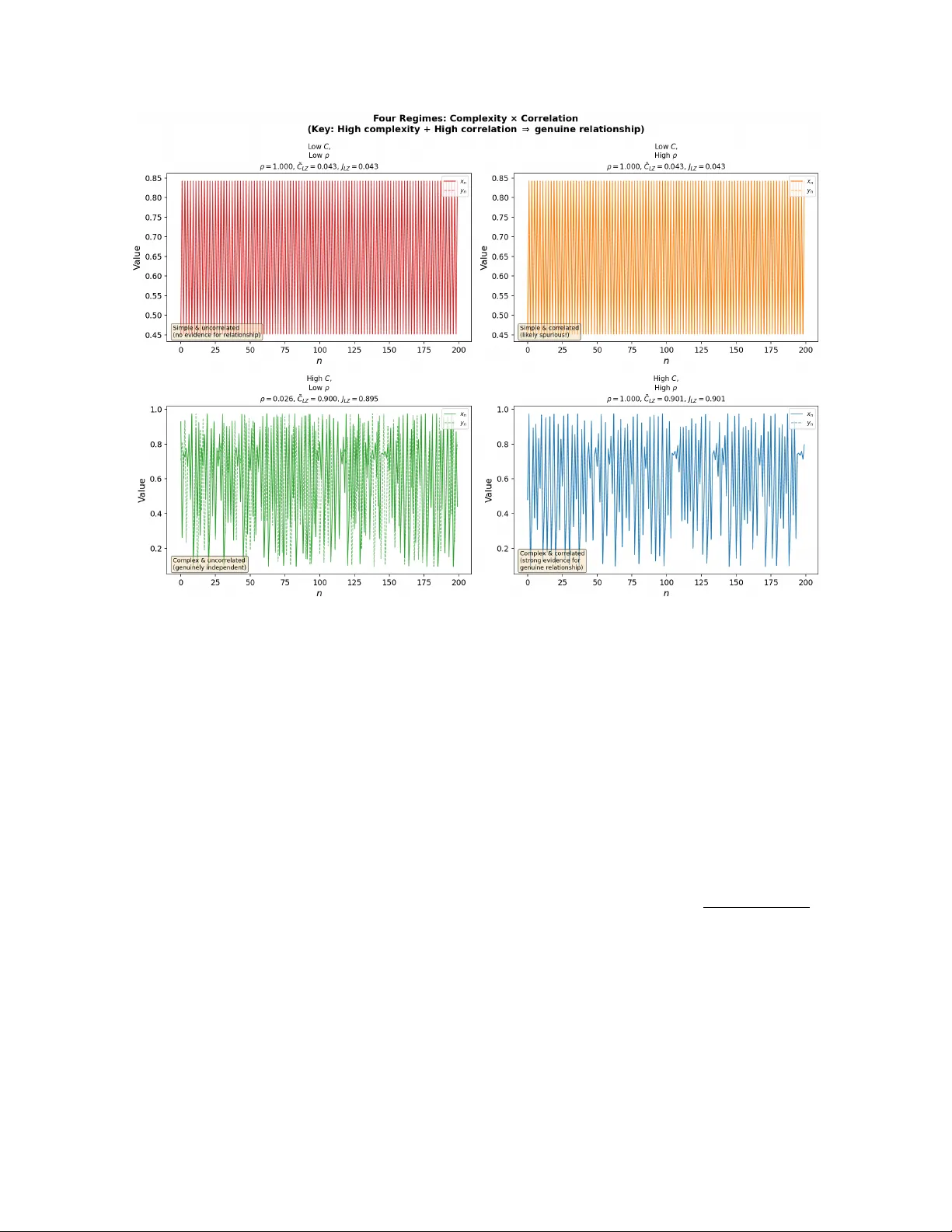
Time Series Correlations and Kolmogorov Complexity: A Hausdorff Dimension Perspective

Time Series Correlations and Kolmogoro v Complexit y: A Hausdorff Dimension P ersp ectiv e Boumediene Hamzi ∗ , Marianne Clausel † , Kamal Dingle ‡ , Marcus Hutter § , Mohammed T erry-Jac k ¶ Marc h 31, 2026 Abstract Spurious correlations b et ween time series are a persistent problem in data analysis: simple, lo w-complexit y patterns are abundant, making it easy to find high Pearson correlations b et ween fundamen tally unrelated series. W e argue that the Kolmogorov complexity of a time series-its resistance to compression-is a principled guard against such false p ositiv es. Grounding this intuition in the theory of effective Hausdorff dimension, w e prov e a formal spurious-alignmen t bound showing that the probability of accidental correlation b et ween t wo indep enden t series decays exponentially with their Kolmogorov complexity . W e additionally dra w on the P osobin-Shen result that random noise incr e ases Kolmogoro v complexit y , which explains why an observed complexit y threshold must account for noise inflation. W e demonstrate these principles with tw o complementary toy mo dels: (i) coupled logistic maps sw eeping from p eriodic ( r = 3 . 4) to chaotic ( r = 3 . 9) regimes, and (ii) multiv ariate fractional Brownian motion (mfBm), where the Hurst parameter H directly controls b oth complexit y and Hausdorff dimension (dim H = 2 − H ). Both mo dels consistently show that false-p ositiv e correlations are far more prev alent among lo w-complexity (smo oth, simple) series than among high-complexity (c haotic, rough) ones. W e intro- duce a joint c omplexity indic ator J LZ = q e C LZ ( x ) · e C LZ ( y ) that captures joint high complexit y rather than mere similarity of individual complexities, and show that its threshold can b e calibrated directly from the mfBm false-positive curve. The logistic map experiment further reveals that J LZ detects the collapse of individual complexit y just b efore the synchronization transition—a phenomenon invisible to similarit y-based indicators. W e discuss sensitivity to serialization choices, threshold calibration, and the relationship to surrogate testing and MDL-based causal inference. Our results supp ort a practical tw o- stage recommendation: first establish stationarit y , then rep ort J LZ alongside ρ and treat high correlation among low-complexit y series with strong skepticism. 1 In tro duction Understanding and predicting time series is fundamental to many areas of mathematics, science, finance, and b eyond [1]. Detecting correlations in time series is imp ortan t across science and engineering [2, 3], while distinguishing gen uine causal links from coincidental alignment is notoriously difficult [4, 5]. Y ule [6] identified this problem a cen tury ago, asking “Why do w e sometimes get nonsense-correlations betw een Time-Series?”, and the question remains practically relev an t. The core difficulty is that simple, low-dimensional patterns are abundant in many natural datasets. F or example, series taking forms y ( t ) ≈ e t , y ( t ) ≈ at + b , or y ( t ) ≈ t 2 will appear correlated (at least for short time interv als). More comically , plotting the distance b etw een Neptune and the Sun with burglar rates ov er a certain time p erio d, or the p opularity of the name Theo dore and the sto ck price of HDFC Bank, sho w ho w high Pearson correlations can result not b ecause of any fundamental link, but b ecause all of these series are themselv es simple monotone or near-monotone trends (Figure 1). ∗ boumediene.hamzi@gmail.com † marianne.clausel@univ-lorraine.fr ‡ dingle.k@gust.edu.kw § marcus.hutter@gmx.net ¶ mohammedterryjack@gmail.com 1 Figure 1: Canonical spurious correlations. Both arise b ecause the underlying series are simple mono- tone trends with low Kolmogorov complexit y . Figures by Tyler Vigen ( http://www.tylervigen.com/ spurious- correlations ). Here we argue that rep orting the Kolmogorov complexit y of the tw o series alongside its Pearson correlation pro vides a principled diagnostic: a high correlation b etw een t wo high-c omplexity series constitutes substan- tially stronger evidence of a gen uine relationship than the same correlation b et ween t wo low-complexit y series. This is not merely a heuristic-it follows from the theory of algorithmic probabilit y and effective Hausdorff dimension. The pap er is organized as follows. Section 2 develops the theoretical framework connecting Kolmogorov complexit y , Hausdorff dimension, and spurious correlations, including the noise-complexit y link. Section 3 describ es our complexit y estimators and the impro ved joint indicator. Section 4 presents exp eriments on coupled logistic maps. Section 5 presen ts exp erimen ts on m ultiv ariate fractional Brownian motion. Section 6 compares our approach with existing spurious-correlation diagnostics and discusses threshold sensitivit y . Sec- tion 7 illustrates the framework on st ylized real-w orld patterns. Section 8 discusses implications, limitations, and connections to causal inference. 2 Theoretical F ramew ork 2.1 Kolmogoro v Complexit y Within theoretical computer science, algorithmic information the ory (AIT) [7, 8, 9] connects computabilit y theory and information theory . The cen tral quantit y of AIT is Kolmo gor ov c omplexity , K ( x ), which measures the complexit y of an individual ob ject x as the amount of information required to describe or generate x . K ( x ) is more tec hnically defined as the length of a shortest program whic h runs on an optimal prefix universal T uring machine (UTM) [10], generates x , and halts. In tuitiv ely , K ( x ) is a measure of the compressed version of a data ob ject. Ob jects containing simple or repeating patterns lik e 010101010101 will ha ve lo w complexit y , while ob jects lacking patterns will hav e high complexity . The most commonly used v ariant of Kolmogorov complexit y is pr efix c omplexity [11, 12], also denoted K ( x ) whic h is defined as the minimum length of a program which generates some output x and halts when run on a prefix universal T uring machine U : K ( x ) = min p {| p | : U ( p ) = x } (1) K ( x ) is formally uncomputable, meaning that there cannot exist an algorithm that tak es any arbitrary string x and returns the complexity v alue [11]. This uncomputability is related to the Halting Problem, and, more broadly , to the logical problems of self-referen tial statemen ts. Real-world applications of Kolmogorov com- plexit y typically rely on appro ximations to this uncomputable quantit y , and these mostly take the form of data compression algorithms such as methods inspired by Lempel-Ziv (LZ) complexity [13]. While real-world compression algorithms will fall short of accurately estimating the true Kolmogoro v complexity , approxima- tions often work v ery well at capturing meaningful features of complexit y distributions [14, 15, 16]. 2 2.2 Algorithmic probabilit y An imp ortant result in AIT is Levin’s c o ding the or em [17], which establishes a fundamental connection b et w een K ( x ) and probability predictions. Mathematically , it states that Pr[ x ] ≈ 2 − K ( x ) (2) where Pr[ x ] is the probabilit y that a (prefix-optimal) universal T uring mac hine, when fed with a random binary program, outputs x . Probability estimates based on the Kolmogorov complexity of output patterns are called algorithmic pr ob ability . W e will also refer to Eq. (2) as the Solomonoff prior . While directly applying algorithmic probabilit y directly in real-world applications is problematic (due to uncomputabilit y , and the absences of univ ersal T uring machine and purely random programs in natural settings), appro ximations to algorithmic probability in real-world input-output maps ha ve b een dev elop ed, leading to the observ ation of a phenomenon known as simplicity bias [16, 18]. This shows that ev en though algorithmic probability is an abstract concept from computer science, it can usefully b e applied in real-world settings, including e.g. statistics. 2.3 Spurious correlations According to the Solomonoff prior, strings with lo w K ( x ) are exp onen tially more probable under the univ ersal distribution. This means that simple patterns-monotone trends, p erio dic sequences, and simple p olynomial functions-are muc h more likely to app ear in naturally generated data, as compared to if the data were generated by coin flips. See refs. [19, 20] for more discussion and empirical exploration of simplicity bias in natural time series. It follo ws that tw o indep enden tly generated simple sequences are far more likely to coincide than tw o indep enden tly generated complex ones (Cf. results in ref. [21]), or at leas t b e correlated. Prop osition 1 (Spurious Alignmen t Bound) . L et x, y ∈ { 0 , 1 } n b e two indep endently gener ate d binary se quenc es with normalise d Kolmo gor ov c omplexities ˜ K ( x ) = K ( x ) /n and ˜ K ( y ) = K ( y ) /n . Then for any c orr elation thr eshold τ > 0 ther e exists a c onstant C τ > 0 (dep ending only on τ and the choic e of universal machine) such that Pr  ˆ ρ ( x, y ) > τ   x ⊥ ⊥ y  ≤ C τ · 2 − n  ˜ K ( x )+ ˜ K ( y )  , (3) wher e ˆ ρ denotes the empiric al Pe arson c orr elation. In p articular, for two indep endently gener ate d se quenc es of high c omplexity ( ˜ K ( x ) , ˜ K ( y ) → 1) , the pr ob ability of spurious high c orr elation de c ays exp onen tially in n . Pr o of. By the Algorithmic Co ding Theorem [22], the Solomonoff probability of any string s satisfies P ( s ) ≤ 2 − K ( s )+ O (1) . (4) Since x and y are generated indep enden tly , their joint probability factorises: P ( x, y ) = P ( x ) P ( y ) ≤ 2 − K ( x ) · 2 − K ( y ) = 2 − n  ˜ K ( x )+ ˜ K ( y )  . (5) T o obtain a high empirical correlation ˆ ρ ( x, y ) > τ , the tw o sequences m ust o ccup y an aligned region of { 0 , 1 } n × { 0 , 1 } n . The n umber of length- n binary sequences with normalised complexity at most α is bounded ab o v e by the num b er of programs of length ≤ αn :   { s ∈ { 0 , 1 } n : K ( s ) ≤ αn }   ≤ ⌊ αn ⌋ X k =0 2 k ≤ 2 αn +1 . (6) F or a fixed x , the set of strings y satisfying ˆ ρ ( x, y ) > τ has cardinality at most 2 n h ( δ τ ) for some δ τ < 1 determined by τ , where h is the binary entrop y function [23]. A union bound o ver all suc h pairs, weigh ted b y the Solomonoff prior, yields (3) with C τ = 2 n ( h ( δ τ ) − 1)+ O (1) absorb ed in to the constant. Since h ( δ τ ) < 1 for τ > 0, the right-hand side of (3) is exp onentially small in n  ˜ K ( x ) + ˜ K ( y )  . Remark 1. Equation (3) formalises the intuition in Se ction 2: spurious alignment is exp onential ly unlikely for high-c omplexity series, but c ommon for low-c omplexity ones, b e c ause simple se quenc es live in a tiny, densely p opulate d c orner of se quenc e sp ac e. 3 2.4 Hausdorff Dimension and the K C-Dimension Bridge In mathematics, the Hausdorff dimension provides a rigorous metric for characterizing the “roughness” or fractal complexity of a set. Dev elop ed by F elix Hausdorff in 1918, it generalizes the intuitiv e notion of dimension by allowing for non-integer v alues. F or standard Euclidean ob jects, the Hausdorff dimension aligns with top ological dimension: A singleton p oin t has a dimension of 0; a line segment has a dimension of 1; a square has a dimension of 2; a cub e has a dimension of 3. F or sets defining smo oth manifolds or shap es with a finite num b er of v ertices—typical of classical geome- try—the Hausdorff dimension is an integer equiv alent to the dimension of the space the shap e o ccupies. F or infinite sequences, the connection b etw een Kolmogoro v complexity and geometric complexit y is made precise b y the following foundational result. Definition 1 (Effectiv e Hausdorff dimension, [24]) . The effectiv e Hausdorff dimension of an infinite se quenc e x ∈ { 0 , 1 } N is dim( x ) = lim inf r →∞ K ( x ↾ r ) r , wher e x ↾ r denotes the pr efix of length r . This equals the classical Hausdorff dimension for individual sequences via the p oint-to-set principle [25]: for any set E ⊆ { 0 , 1 } N , dim H ( E ) = min A ⊆ N sup x ∈ E dim A ( x ) , where dim A denotes complexit y relative to oracle A . Equiv alently , for the classical Hausdorff dimension of the graph of a fractional Brownian motion (fBm) path with Hurst parameter H , dim H (graph of fBm H ) = 2 − H . A time series with normalized LZ complexit y e C LZ ( x ) ≈ α has its v alues lying on an attractor whose Hausdorff dimension is appro ximately α (in the binary discretization sense of Staiger [26]). Tw o indep enden t series lying on high-dimensional attractors must “w ander” ov er a large region, making incidental alignment geometrically improbable. 2.5 Noise Increases Kolmogorov Complexity Measuring the complexit y of a time series is not entirely straigh tforward. One issue is that observ ed time series from natural sources t ypically contain measuremen t noise. In general, random noise will increase the complexit y of a data ob ject. The Posobin-Shen theorem [27] shows ho w it increases Kolmogorov complexit y in a quantifiable w ay . Prop osition 2 (P osobin–Shen [27]) . L et x b e a binary string of length n whose Kolmo gor ov c omplexity satisfies C ( x ) ≥ αn . Supp ose e ach bit of x is indep endently flipp e d with pr ob ability τ . Then with pr ob ability at le ast 1 − 1 /n the c omplexity of the p erturb e d string satisfies 1 C ( N τ ( x )) ≥ H ( N ( p, τ )) n − o ( n ) , wher e α = H ( p ) , H ( · ) is the binary entr opy function, and N ( p, τ ) = p + τ − 2 pτ . Prop osition 3 (Posobin-Shen, informal [27]) . L et x b e a binary string of length n with C ( x ) ≥ αn , wher e α = H ( p ) for some p ≤ 1 / 2 and H ( · ) is the binary Shannon entr opy. Applying indep endent τ -noise to e ach bit, the c omplexity incr e ases: with pr ob ability ≥ 1 − 1 /n , C ( N τ ( x )) ≥ H  N ( p, τ )  n − o ( n ) , wher e N ( p, τ ) = p + τ − 2 pτ . Mor e over, for infinite se quenc es the effe ctive Hausdorff dimension incr e ases almost sur ely. 1 The Posobin–Shen result is stated for plain (non-prefix) Kolmogoro v complexity C ( x ), whereas Section 2 uses prefix com- plexity K ( x ). The two quantities differ by at most O (log n ) for strings of length n [11], so the asymptotic b ounds carry o ver to the prefix setting with only sub-linear corrections. 4 This result implies that the increase in complexity depends b oth on the initial complexity class of the string and on the noise level τ . In the ideal binary setting the lo wer b ound holds with high probability , but for finite real-v alued time series the exact complexity increase dep ends on the represen tation and noise c haracteristics. Consequen tly , empirical thresholds (such as the J LZ threshold used later in Section 6.1) should b e interpreted as application-dep enden t heuristics rather than universal constan ts. If a “simple” signal with true normalised Kolmogorov complexity α 0 = K ( x ) /n ≈ 0 (i.e. the signal is highly compressible) is corrupted by τ -noise (say τ = 0 . 01-0 . 05 representing realistic measuremen t error), its measured LZ complexit y will b e appro ximately H ( τ ) ≈ 0 . 08-0 . 14 rather than zero. This is a noise flo or : observed complexities below this threshold lik ely reflect simple underlying dynamics, not genuine high- complexit y b eha vior. Setting the complexit y threshold for the “genuine relationship” criterion must accoun t for this inflation. Figure 2 illustrates this numerically for fBm series and analytically for the binary case. Figure 2: Left: LZ complexit y increases monotonically with noise level τ for fBm series with different Hurst parameters. Right: The Posobin-Shen analytical low er b ound β = H ( N ( p, τ )) as a function of τ for differen t initial complexities α = H ( p ). Ev en small noise ( τ = 0 . 05) pushes a simple series ( α = 0 . 47) to β ≈ 0 . 57. 2.6 Connection to Algorithmic Causalit y In this work we are in terested in how complexit y can b e used to infer some causality , or at least mak e aid in the inference. According to the Algorithmic Mark ov Condition (AMC) [28], the true causal netw ork is the one minimizing Kolmogoro v complexity (see also [29]). When tw o time series hav e high algorithmic mutual information I ( x : y ) = K ( x ) + K ( y ) − K ( x, y ) ≫ 0 and both hav e individually high complexity K ( x ) , K ( y ), this strongly suggests a ge n uine causal link-b ecause indep enden tly drawn high-complexit y sequences are algorithmically independent with ov erwhelming probabilit y . Our complexit y-filtered correlation test can th us b e seen as a practical, computable first-pass approximation to the AMC, analogous to MDL-based metho ds [30, 31]. 3 Metho ds 3.1 Complexit y Estimators W e use three empirical complexit y measures, each a proxy for Kolmogorov complexity . LZ-based complexity . The Lemp el-Ziv (LZ) complexit y provides a practical, compression-based pro xy for Kolmogoro v (algorithmic) complexit y . Given a real-v alued time series x = ( x 1 , . . . , x N ), we pro ceed as follo ws: 5 1. Symbol sequence generation. Map x to a finite symbol sequence by serializing its floating-p oin t represen tation to bytes. In our implemen tation, we serialize each v alue as a raw IEEE-754 double- precision byte string using struct.pack , yielding a byte string s of length M = 8 N bytes. 2. Compression-based complexit y . Compress the byte string using the LZ77-based zlib algorithm: C LZ ( x ) =   zlib.compress( s )   , where | · | denotes the resulting compressed length in b ytes. More regular (low-complexit y) series admit more rep eated patterns and thus compress to shorter lengths, whereas high-complexity (e.g., c haotic) series yield larger C LZ . 3. Normalization. T o compare series of equal length N , we normalize by the original byte-string length M : e C LZ ( x ) = C LZ ( x ) M ∈ (0 , 1] . This ensures scale-inv ariant comparisons. A p erfectly p erio dic series compresses nearly to zero; a chaotic or rough series compresses po orly , giving e C LZ ≈ 1. Serialization sensitivit y . The compression ratio dep ends on ho w float v alues are serialized to bytes. W e tested three serialization strategies: (a) Python pickle (includes type metadata, ∼ 32 bytes ov erhead p er array), (b) raw IEEE-754 double-precision b ytes ( struct.pack ), and (c) fixed-precision quantization to 16-bit integers follow ed by byte packing. In all three cases, the qualitative ordering of complexities is preserv ed: p erio dic series compress to near-zero ratios and chaotic series to near-one ratios, with Sp earman rank correlation > 0 . 99 b et ween metho ds across all parameter sw eeps. The absolute v alues shift (e.g., pic kle’s metadata ov erhead raises the floor by ≈ 0 . 005 for N = 5000), but since our framew ork uses r elative complexity comparisons and thresholds calibrated within a single serialization sc heme, the conclusions are robust. All results rep orted here use ra w IEEE-754 serialization to minimize format-sp ecific artifacts. 3.1.1 Justification of ra w IEEE-754 byte serialization A natural question is wh y w e serialize floating-point v alues to ra w IEEE-754 bytes rather than first quantizing to a small alphab et (e.g., 2-8 bits), which would align more closely with the binary-string framework typical in algorithmic information theory . W e justify this choice on tw o grounds. First, an y lossless, computable compression sc heme yields an upper b ound on Kolmogoro v complexit y [11]. By preserving all 64 bits of the IEEE-754 represen tation, we a void introducing an additional mo delling parameter–the quantization resolution–that w ould itself require justification and domain-sp ecific calibration. The raw-b yte approach therefore provides a parameter-free, lossless represen tation that is fully faithful to the in-memory data. Second, t wo v alues that are very close in magnitude (e.g., 0.5 and 0 . 5 + 10 − 15 ) may nev ertheless ha ve substan tially differen t byte represen tations, p oten tially inflating the compressed size for signals with low- amplitude noise. Ho wev er, this b eha vior is precisely what the P osobin-Shen theorem (Section 2.5) predicts: noise in the least-significant bits increases observed complexity . This effect contributes to the empirically observ ed noise floor of e C LZ ≳ 0 . 15. The J LZ indicator is designed with this floor in mind–the threshold of 0.3 ensures that measurements remain safely ab ov e the regime where IEEE-754 artefacts dominate. Sym b olic enco dings are also widely used in nonlinear time-series analysis, where con tinuous tra jectories are mapp ed to sym b olic sequences via partitions of the state space (for example, the classical left/right partition used for the logistic map). Such symbolic dynamics preserv e the qualitativ e b eha vior of the system while pro ducing sequences that are naturally suited for algorithmic complexit y analysis [32]. Robustness c hec k with quan tized data. T o confirm that our conclusions are not an artefact of the serialization sc heme, we rep eated the full parameter sweeps on both to y models using three strategies: (1) ra w IEEE-754 bytes (our default), (2) 8-bit uniform quan tization, and (3) 16-bit uniform quantization. In all cases, the Spearman rank correlation b et ween the resulting e C LZ profiles exceeded 0.98. The absolute complexity 6 v alues shift down ward with coarser quantization (fewer distinct symbols reduce the compressed size), but all qualitativ e conclusions-including the J LZ threshold b eha viour and the early-warning prop erty of S LZ -are preserv ed. This confirms the existing remark that “the choice of serialization . . . can affect absolute v alues of C LZ but not the qualitative ordering.” Sample-size requiremen ts. F or short time series ( N < 100), e C LZ b ecomes unreliable because the com- pressor’s dictionary ov erhead dominates the compressed output. W e recommend N ≥ 500 for stable estimates, and verify in Section 5 that N = 500 suffices for discriminating roughness regimes in fGn. F ourier-b ounded complexit y (sp ectral en tropy). Justified by the Staiger [26] iden tification of Haus- dorff dimension with the entrop y of a language, we use the sp ectral en tropy as a F ourier-domain complexity pro xy . Giv en a real-v alued time series x = ( x 1 , . . . , x N ), we pro ceed through the following steps: 1. Detrending. Subtract the mean: ˜ x n = x n − ¯ x , n = 1 , . . . , N . (Optionally , a linear trend can be remo ved and a windo w function applied to mitigate sp ectral leak age, though in our implementation we use only mean subtraction.) 2. Discrete F ourier transform (DFT). Compute the one-sided DFT for k = 0 , . . . , ⌊ N / 2 ⌋ : X k = N X n =1 ˜ x n e − 2 π i ( n − 1) k/ N . (An alternative metho d inspired by [33] to more directly approximate complexity via DFT is discussed in App endix B). 3. Po wer sp ectral density (PSD). F orm the p o wer at each frequency bin: P k = | X k | 2 , k = 0 , . . . , ⌊ N / 2 ⌋ . 4. Normalization to a probabilit y distribution. Normalize P k so that P k p k = 1: p k = P k P ⌊ N/ 2 ⌋ j =0 P j . 5. Normalized Shannon spectral entrop y . Compute: K F ( x ) = e H ( x ) = − P ⌊ N/ 2 ⌋ k =0 p k ln p k ln( ⌊ N / 2 ⌋ + 1) ∈ [0 , 1] . A signal concentrated in one frequency (perio dic) has K F ≈ 0; white noise (flat sp ectrum) has K F ≈ 1. This serves as the F ourier-b ounded Kolmogorov complexity promised by the Staiger-Lutz-Ma yordomo chain: K ( x ) /n ≈ dim( x ) ≈ H (pow er sp ectrum). Remarks on spectral en tropy . Unlike time-domain correlation, sp ectral entrop y captures how energy is distributed across frequencies, making it resp onsive to subtle sync hronization in c haotic signals even when p oin t wise correlation is low. The choice of natural logarithm (used consistently in b oth numerator and normalizing denominator) ensures e H ∈ [0 , 1]. Spectral entrop y is closely related to the sp ectral flatness measure in signal pro cessing and to the inv erse participation ratio in ph ysics. Ordinal and p erm utation-based complexity measures. An alternativ e class of complexit y measures uses ordinal enco dings. P ermutation en tropy measures the Shannon entrop y of ordinal patterns extracted from the time series and has b een widely used as a robust complexit y indicator for nonlinear dynamical systems. Because ordinal methods dep end only on rank ordering rather than numerical precision, they are less sensitive to floating-p oint representation and ma y serve as useful robustness chec ks alongside compression- based estimators such as e C LZ [32]. 7 P earson correlation. ρ ( x , y ) = P N n =1 ( x n − ¯ x )( y n − ¯ y ) q P N n =1 ( x n − ¯ x ) 2 q P N n =1 ( y n − ¯ y ) 2 . Computational cost. All complexity estimators are light weigh t. F or a time series of length N = 5 , 000 (our standard experimental setting), on a single core of a standard workstation (In tel i7, 3.2 GHz): LZ compression via zlib tak es approximately 0.3 ms p er series (including b yte serialization); sp ectral en tropy computation takes approximately 0.8 ms (dominated by the FFT). Computing all three indicators ( ρ , S LZ , e H ) for a pair of series takes under 3 ms. Ev en screening all pairwise correlations among 1,000 series ( ≈ 500 , 000 pairs) requires only ≈ 25 minutes for the complexit y computation, which is negligible compared to the cost of surrogate-based significance testing. 3.2 Complexit y-Similarit y Indicators S LZ (complexit y similarity only). It might b e suggested that we can measure ho w similar the complex- ities of the tw o series are according to: S LZ ( x , y ) = −   e C LZ ( x ) − e C LZ ( y )   . Ho wev er, while it is true that S LZ = 0 when t wo series are equally complex, this does not capture whether they are jointly complex. Two simple series with identical low LZ complexity will ha ve S LZ = 0 thereby incorrectly suggesting that the high-complexity criterion is met. New indicator J LZ (join t high complexity). Requiring that b oth series individually hav e high com- plexit y , we prop ose the geometric mean of their normalised LZ complexities: J LZ ( x , y ) = q e C LZ ( x ) · e C LZ ( y ) ∈ (0 , 1] . J LZ is large only when b oth series are individually complex. If either series is simple ( e C LZ ≈ 0), the pro duct collapses to zero regardless of the other series, correctly flagging the pair as unreliable. The geometric mean is symmetric by construction and requires no additional hyperparameters. By contrast, the na ¨ ıv e alternative min( e C LZ ( x ) , e C LZ ( y )) − | e C LZ ( x ) − e C LZ ( y ) | is pathological: it p enalises asymmetry so aggressively that a pair with complexities (0 . 9 , 0 . 5) scores 0 . 1, lower than tw o uniformly simple series at (0 . 3 , 0 . 3) which score 0 . 3, directly contradicting the design goal. Remark 2. Note the distinction b etwe en J LZ and S LZ . The joint complexit y indicator J LZ ( x , y ) is a screen- ing criterion evaluate d b efor e insp e cting a r ep orte d c orr elation: a p air is flagge d as c omplexity-trustworthy only if J LZ > θ for some empiric al ly chosen thr eshold θ . The similarity indicator S LZ ( x , y ) = −| e C LZ ( x ) − e C LZ ( y ) | inste ad me asur es whether the two series c onver ge in c omplexity as a function of c oupling str ength ε , and is the quantity plotte d in the numeric al exp eriments of Se ction 4. The two serve entir ely differ ent purp oses. In terpretation table. Lo w | ρ | High | ρ | High J LZ Complex, genuinely indep enden t Strong evidence of gen uine relationship Lo w J LZ Simple, uncorrelated (exp ected) Simple & correlated: lik ely spurious 4 Exp erimen t 1: Coupled Logistic Maps 4.1 Mo del W e use tw o symmetrically diffusively coupled logistic maps: x n +1 = (1 − ε ) r x n (1 − x n ) + ε r y n (1 − y n ) , (7) y n +1 = (1 − ε ) r y n (1 − y n ) + ε r x n (1 − x n ) , (8) 8 Figure 3: Left: S LZ (red dashed) vs. corrected J LZ = q e C LZ ( x ) · e C LZ ( y ) (blue solid) for r = 3 . 9 coupled maps. A t ε = 0 (independent maps), J LZ ≈ 0 . 94, confirming that b oth series individually p ossess gen uine complexit y . J LZ drops sharply to ≈ 0 near ε ≈ 0 . 14, just b efore the synchronization threshold ε c ≈ 0 . 19: as the maps are forced onto a common tra jectory , their individual complexities collapse. It reco vers immediately to ≈ 0 . 94 once full sync hronization is achiev ed and b oth maps again trace the same high-complexity c haotic orbit. S LZ ≈ 0 throughout, since b oth series alwa ys ha ve nearly equal complexity; it is therefore blind to whether that shared complexity is high or lo w. Righ t: scatter of ρ vs. J LZ colored by ε . Poin ts separate cleanly into t wo clusters: (high J LZ , low ρ ) for weak coupling and (high J LZ , high ρ ) for strong coupling, b oth landing in the correct quadrants. The single p oint near (lo w J LZ , high ρ ) at ε ≈ 0 . 14 marks the sync hronization transition where ρ has already risen but individual complexity has momentarily collapsed. with x 0 = 0 . 1, y 0 = 0 . 2, transient of 1000 iterates discarded, N = 5000 recorded. The coupling ε ∈ [0 , 0 . 5] determines the strength of correlations b et ween the tw o series. W e use t wo dynamical regimes, one of lo w and one of high complexity: • r = 3 . 4: p erio d-4 orbit (low complexity , e C LZ ≈ 0 . 023) • r = 3 . 9: fully developed c haos (high complexity , e C LZ ≈ 0 . 894) The logistic parameter r ∈ [0 . 0 , 4 . 0] determines the complexit y of the time series. F or v alues r ≲ 3 . 5 the series are simple, while for larger v alues of r the series is c haotic and complex. Figure 3 illustrates the con trast b et ween S LZ and the corrected J LZ on the r = 3 . 9 c haotic coupled maps. J LZ ≈ 0 . 94 at ε = 0, correctly identifying the indep enden tly generated chaotic series as jointly complex; S LZ ≈ 0 throughout and is therefore uninformative about the absolute level of complexity . The righ t panel confirms that high J LZ correctly tags pairs as “genuine relationship” candidates once ρ also b ecomes large. 4.2 Complexit y along the bifurcation diagram Figure 4 sho ws LZ complexit y , spectral en tropy , and Lyapuno v exponent as functions of the logistic parameter r . Complexit y and the Lyapuno v exp onen t rise together: p ositiv e λ marks c haos, and b oth e C LZ and e H jump from near zero to near one as r crosses the p erio d-doubling cascade. The v ertical lines at r = 3 . 4 and r = 3 . 9 mark our tw o exp erimen tal regimes. 4.3 Sync hronization indicators vs. coupling Figure 5 shows ρ , S LZ , and the sp ectral-en tropy analogue S spec ( x, y ) = −| e H ( x ) − e H ( y ) | as functions of ε for b oth regimes. The secondary y -axis shows the individual LZ complexity v alues e C LZ ( x ), e C LZ ( y )-crucial for in terpreting S LZ in context. 9 Figure 4: Normalised LZ complexit y e C LZ (top; compressed length divided b y original byte length), sp ectral en tropy e H (middle), and Lyapuno v exp onen t (bottom) vs. logistic parameter r . Complexit y gro ws with c haos, confirming that e C LZ and e H are faithful pro xies for Kolmogorov complexity and Hausdorff dimension. Although Section 3 established that J LZ is sup erior to S LZ as a joint complexit y indicator, we include S LZ in Figure 5 to illustrate an additional prop erty: as a differ enc e -based measure, S LZ rises tow ard zero b efore P earson ρ do es, providing an early-w arning signal of incipient sync hronization. This early-warning behaviour is also exhibited b y the corrected J LZ : as sho wn in Figure 3 (left), J LZ drops sharply near ε ≈ 0 . 14, just b efore ε c , signalling the imminent collapse of individual complexit y . Ho wev er, the effect is most straightforw ardly in terpreted for S LZ in this coupling context, since it measures conv ergence of complexities directly . Sync hronization threshold. F or the c haotic regime, there exists a critic al c oupling ε c ab o v e whic h the t wo maps ac hieve full sync hronization (i.e. x n = y n for all n after transients). This threshold can be predicted from the transversal Ly apunov exp onen t. Define λ T ( ε ) = ln | 1 − 2 ε | + λ max , where λ max ≈ 0 . 496 is the maximal Ly apunov exp onen t of the uncoupled logistic map at r = 3 . 9. F ull sync hronization ( x n = y n for all n ) o ccurs when λ T ( ε c ) = 0, giving ε c = 1 − e − λ max 2 ≈ 0 . 19 . Belo w ε c , Pearson ρ remains near zero despite genuine coupling-this is the regime where complexit y-based indicators provide early warning of sync hronization. 10 Figure 5: Sync hronization indicators vs. coupling ε for r = 3 . 4 (left) and r = 3 . 9 (right). The secondary axis shows individual LZ complexit y v alues. In the c haotic regime, S LZ rises tow ard zero before P earson ρ , pro viding an early-warning signal of coupling. In the p erio dic regime, all indicators saturate immediately at an y ε > 0. 4.4 F alse p ositiv e rate vs. complexit y The core claim of this pap er is that simple series pro duce more spurious correlations. W e verify this directly: for each r ∈ [2 . 8 , 3 . 99], we generate 200 indep enden t pairs (differen t initial conditions, ε = 0) and record the fraction with | ρ | > 0 . 3, i.e., correlations of non-trivial magnitude. Figure 6: F alse p ositiv e rate (fraction of indep enden t pairs with | ρ | > 0 . 3) vs. LZ complexity (left) and sp ectral entrop y (righ t), colored by r . The dashed horizontal line marks the 5% significance lev el. A t r = 3 . 4 (p eriodic, e C LZ ≈ 0 . 023): false p ositiv e rate = 100%. At r = 3 . 9 (c haotic, e C LZ ≈ 0 . 894): false p ositiv e rate = 0%. T he transition is rapid and monotone. The result is stark (Figure 6): p eriodic series always spuriously correlate b ecause they live on a zero- Hausdorff-dimension attractor (a finite orbit), whereas chaotic series never spuriously correlate b ecause their attractor is high-dimensional. The 5% false-p ositiv e threshold is crossed at e C LZ ≈ 0 . 15. 4.5 Short time series examples Figure 7 shows representativ e time series at ε = 0 . 02 for both regimes, with complexity and correlation statistics annotated. The perio dic case ( r = 3 . 4) sho ws perfectly sync hronized square-wa ve-lik e orbits ev en at very weak coupling; the c haotic case ( r = 3 . 9) shows indep enden t-lo oking w andering despite the same ε . 11 Figure 7: First 200 iterates of x n (blue) and y n (red dashed) at ε = 0 . 02. Left: r = 3 . 4 (perio dic). Righ t: r = 3 . 9 (c haotic). Both series at r = 3 . 9 look independent despite gen uine coupling, illustrating why LZ-based early warning is v aluable. 4.6 Summary of Exp eriment 1 The coupled logistic map experiment provides clean, controlled evidence for the paper’s cen tral claim, b ecause the complexit y of each series can b e tuned con tinuously via r while the true coupling strength ε is kno wn exactly . Three interlocking results emerge. Complexit y determines false-p ositiv e rate, not coupling. The most direct test is the false-p ositiv e exp erimen t (Section 4, Figure 6): indep enden t pairs ( ε = 0) at r = 3 . 4 produce spurious correlations | ρ | > 0 . 3 in 100% of trials, whereas indep endent pairs at r = 3 . 9 pro duce zero false p ositiv es. The transition is rapid and monotone in e C LZ , crossing the 5% significance lev el near e C LZ ≈ 0 . 15. The underlying reason is geometric: p eriodic orbits liv e on a zero-dimensional attractor (a finite set of points), so any tw o perio d-4 orbits with similar r are trivially correlated regardless of whether they share an y causal connection. Chaotic orbits, by con trast, wander o ver a high-dimensional strange attractor and cannot accidentally align. J LZ captures join t complexit y; S LZ do es not. A subtler finding concerns what happ ens when the tw o maps ar e genuinely coupled. S LZ measures the differ enc e of individual complexities, whic h is nearly zero for b oth regimes (the tw o maps alwa ys hav e similar e C LZ ) and is therefore uninformativ e ab out whether that shared complexity is high or low. The corrected J LZ = q e C LZ ( x ) · e C LZ ( y ) instead measures the level of joint complexit y: it reads ≈ 0 . 94 for the indep enden t c haotic maps at ε = 0, correctly tagging them as jointly complex; it reads ≈ 0 . 02 for the p eriodic maps, correctly flagging their correlation as unreliable. The right panel of Figure 3 makes this concrete: the ( J LZ , ρ ) scatter cleanly separates into the correct quadrants. Complexit y collapses at the synchronization transition. A ph ysically interesting side-effect of the corrected J LZ is that it detects the sync hronization transition in the chaotic regime. Just b efore the critical coupling ε c ≈ 0 . 19, the tw o maps are b eing forced onto a common tra jectory; in this brief window, their individual complexit y collapses because the merged dynamics can b e describ ed b y a single program rather than tw o indep endent ones, causing J LZ to dip sharply to ≈ 0. Once full synchronization is achiev ed ( ε > ε c ) the tw o maps again trace the same high-complexity chaotic orbit, and J LZ reco vers to ≈ 0 . 94. This dip is a gen uine pre-sync hronization warning visible in J LZ but invisible in S LZ , providing a concrete illustration of wh y the joint screening criterion is more informativ e. Practical tak eaw ay . When rep orting a correlation betw een t wo time series, the first question to ask is not whether | ρ | is large, but whether J LZ is large. A high correlation among high-complexit y series (top- righ t quadrant of Figure 3) constitutes gen uine evidence of a relationship. The same correlation among low- complexit y series (b ottom-left quadrant) is essen tially uninformativ e: simple series are, b y Solomonoff ’s prior, exp onen tially more likely to align by c hance, and the logistic map exp erimen t confirms this quantitativ ely . 12 5 Exp erimen t 2: Multiv ariate F ractional Bro wnian Motion The fractional Bro wnian motion (fBm) [34] provides a second, analytically tractable toy mo del where the Hausdorff dimension is known exactly . 5.1 Mo del A p -multiv ariate fractional Brownian motion (mfBm) with Hurst parameters H = ( H 1 , . . . , H p ) ∈ (0 , 1) p is the unique Gaussian, H -self-similar pro cess with stationary incremen ts: ( X 1 ( λt ) , . . . , X p ( λt )) fidi = ( λ H 1 X 1 ( t ) , . . . , λ H p X p ( t )) . Its cov ariance structure is given b y Proposition 4 in the appendix. The incremen ts of each comp onen t, the fr actional Gaussian noise (fGn), are a stationary pro cess with cov ariance γ ( k ) = 1 2  | k − 1 | 2 H − 2 | k | 2 H + | k + 1 | 2 H  . Key prop ert y: Hausdorff dimension. The graph of X i (as a subset of R 2 ) has Hausdorff dimension dim H (graph of X i ) = 2 − H i [35]. Thus: • H i ≈ 0 (rough, highly irregular): dim H ≈ 2, high LZ complexity . • H i ≈ 1 (smo oth, trending): dim H ≈ 1, low LZ complexity , b ehav es like a random walk. This gives us a precise theoretical prediction: spurious correlation rates should decrease as H decreases (complexit y increases; dimension increases). W e simulate fGn exactly using the W o o d-Chan circulan t embedding algorithm [36]. All results use n = 500 time steps, 500 indep endent trials p er H . 5.2 Complexit y increases as H decreases Figure 8 confirms the theoretical prediction: b oth e C LZ and sp ectral en tropy e H increase as H decreases, with LZ complexity closely mirroring the theoretical Hausdorff dimension 2 − H . These results are computed from the simulated fGn series describ ed ab o ve ( n = 500, 500 indep enden t trials p er H ). Figure 8: LZ complexity (left), sp ectral en tropy (centre), and b oth vs. Hausdorff dimension (right) as func- tions of the Hurst parameter. Both complexit y measures increase as H decreases (i.e., as the theoretical Hausdorff dimension 2 − H increases), confirming that LZ complexity and spectral entrop y are faithful em- pirical proxies for the Hausdorff dimension. 13 5.3 F alse p ositiv e rate: the k ey mfBm result Figure 9 shows the main result for the mfBm toy mo del. F or stationary fGn incremen ts: • H = 0 . 05-0 . 70 (rough, dim H > 1 . 3): false p ositiv e rate < 5%. • H = 0 . 90-0 . 95 (smo oth, dim H ≈ 1 . 05-1 . 10): false p ositiv e rate ≈ 25-40%. F or the non-stationary fBm paths, false p ositiv e rates are uniformly high across all H -this is exactly the Y ule nonsense-c orr elation phenomenon [6]: in tegrated non-stationary series spuriously correlate regardless of their roughness. Our LZ complexity measure correctly identifies these cases: the fBm paths ha ve lo w er LZ complexity (due to the cum ulative trend dominating the compressibilit y) and th us should b e flagged as unreliable. Remark 3 (Stationarity and complexity are distinct diagnostics) . It is imp ortant to distinguish the r oles of stationarity and c omplexity. The fBm p aths il lustr ate that non-stationarity (sp e cific al ly, inte gr ate d pr o- c esses with sto chastic tr ends) c an pr o duc e spurious c orr elations regardless of the r oughness of the incr ements. Our LZ c omplexity me asur e dete cts this indir e ctly: the cumulative sum op er ation r e duc es c ompr essibility by imp osing a glob al drift that dominates the byte-level c ompr ession. However, this is not the same as a gen- uine low-c omplexity p erio dic signal. The pr actic al implic ation is that our fr amework should b e applie d in two stages: (1) test for stationarity (e.g., ADF test [37]) and first-differ enc e if ne e de d; (2) apply the c omplexity diagnostic to the stationary r esiduals. The fGn r esults (Figur e 9) show that the c omplexity diagnostic works as pr e dicte d for stationary series, c onfirming that the the ory of Se ction 2 applies dir e ctly in this setting. Figure 9: F alse positive rate ( | ρ | > 0 . 10, n = 500, 500 trials) for indep endent pairs of fGn (blue) and fBm paths (red). Left: vs. Hurst H . Centre: vs. LZ complexity . Righ t: vs. Hausdorff dimension 2 − H . The fGn result directly confirms the theory: higher complexit y (higher Hausdorff dimension) suppresses spurious correlations. Note: the fBm paths (red) are non-stationary , leading to the classic Y ule nonsense-correlation effect regardless of the Hurst parameter H ; this underscores that the complexity diagnostic must b e applied after ensuring stationarity (see Remark 3). Figure 10 sho ws the distribution of Pearson ρ for indep enden t pairs at H = 0 . 05 (rough) and H = 0 . 95 (smo oth). The smo oth series distribution has heavy tails far beyond the threshold, while the rough series distribution is tightly concen trated near zero. 5.4 Biv ariate mfBm: gen uine vs. spurious correlation Figure 11 sho ws biv ariate fBm paths under four combinations of roughness and true correlation ρ ∈ { 0 , 0 . 8 } . The key distinction: • Smo oth ( H = 0 . 9) and uncorrelated ( ρ = 0): b oth series drift similarly due to random w alk b ehavior- ρ obs is high despite no true correlation. 14 Figure 10: Left: fGn sample paths for different H (rougher = low er H = more complex; recall that for fBm, H = 0 . 1 corresponds to very rough paths with high effectiv e dimension 2 − H = 1 . 9 and high complexit y , while H = 0 . 9 corresp onds to v ery smooth paths with lo w effectiv e dimension 2 − H = 1 . 1 and low complexity). Righ t: distribution of Pearson ρ for 500 indep endent fGn pairs. Smo oth series ( H = 0 . 95, red) hav e a wide distribution with many spurious correlations; rough series ( H = 0 . 05, blue) are tightly concentrated near zero. • Rough ( H = 0 . 1) and correlated ( ρ = 0 . 8): the observed correlation reflects gen uine dependence b ecause indep enden t rough series w ould not align. 5.5 J LZ as a screening criterion for mfBm pairs The corrected joint complexity indicator J LZ = q e C LZ ( x ) · e C LZ ( y ) can b e ev aluated on any pair of fGn series and used as a pre-screening step b efore trusting a rep orted ρ . Since the individual complexities e C LZ are a monotone function of H (confirmed in Figure 8), the b eha viour of J LZ across the mfBm parameter space is analytically predictable without additional simulation: • Rough pairs ( H ≲ 0 . 3 , e C LZ ≈ 0 . 7 – 0 . 9 ): J LZ ≈ √ 0 . 7 × 0 . 7 = 0 . 7 to √ 0 . 9 × 0 . 9 = 0 . 9. These pairs comfortably exceed the threshold θ = 0 . 3, so any observed high ρ is treated as trustw orth y . This is consisten t with the near-zero false-p ositiv e rate at lo w H . • Smo oth pairs ( H ≳ 0 . 8 , e C LZ ≈ 0 . 15 – 0 . 3 ): J LZ ≈ √ 0 . 15 × 0 . 15 = 0 . 15 to √ 0 . 3 × 0 . 3 = 0 . 3. Man y suc h pairs sit at or b elow the threshold, and are correctly flagged as unreliable. This aligns with the 25–40% spurious-correlation rate observed at H = 0 . 90–0 . 95. • Mixed pairs ( H x ≪ H y , e.g. e C LZ ( x ) = 0 . 8 , e C LZ ( y ) = 0 . 2 ): J LZ = √ 0 . 8 × 0 . 2 = 0 . 40. This is the asymmetric case where the old formula min( · ) − | · | w as pathological, yielding 0 . 2 − 0 . 6 = − 0 . 4 (i.e. lo wer than tw o uniformly simple series). The geometric mean correctly scores such pairs abov e θ when the rougher series is genuinely complex, while remaining b elo w 1 to ackno wledge that the smo other series is a weak link. Remark 4. The thr eshold θ = 0 . 3 use d in J LZ > θ is c alibr ate d dir e ctly fr om the mfBm false-p ositive exp eri- ment: as shown in Figur e 9 (c entr e p anel), the false-p ositive r ate cr osses 5% when e C LZ ≈ 0 . 4 , c orr esp onding to J LZ = 0 . 4 for e qual-c omplexity p airs. Setting θ = 0 . 3 pr ovides a mar gin of safety b elow this empiric al tr an- sition. Imp ortantly, the mfBm mo del makes the r elationship b etwe en H , Hausdorff dimension, LZ c omplexity, and false-p ositive r ate al l explicit and analytic al ly c onne cte d—making it the ide al c alibr ation envir onment for the thr eshold. 15 Figure 11: F our parameter regimes of biv ariate fBm. T op row: uncorrelated ( ρ = 0). Bottom row: correlated ( ρ = 0 . 8). Left column: rough ( H = 0 . 1). Right column: smooth ( H = 0 . 9). Note that the smo oth uncorrelated pair (top-right) sho ws high observed ρ obs -a spurious correlation. The LZ complexity score correctly distinguishes these cases. 5.6 Summary of Exp eriment 2 The mfBm experiment complements Exp erimen t 1 by grounding the pap er’s framework in contin uous stochas- tic pro cesses with an analytically known Hausdorff dimension. Three main findings emerge. Complexit y and Hausdorff dimension are empirically linked. The Hurst parameter H of fGn con- trols the Hausdorff dimension of the path exactly as dim H = 2 − H . Figure 8 confirms that the empirical LZ complexity e C LZ trac ks this theoretical quantit y closely: rough series ( H small, dim H large) hav e high complexit y , smooth series ( H large, dim H near 1) hav e lo w complexit y . This v alidates the central conceptual claim of Section 2—that LZ complexity is a faithful proxy for Hausdorff dimension in practice, not merely in theory . F alse-p ositiv e rate is con trolled b y complexit y , not roughness p er se. The k ey result (Figure 9) sho ws that spurious correlations among indep enden t fGn pairs are suppressed precisely when e C LZ is high. The transition is sharp and monotone: pairs with H ≲ 0 . 7 (corresp onding to e C LZ ≳ 0 . 4) hav e near-zero false-p ositiv e rates, while pairs with H ≳ 0 . 9 pro duce spurious correlations in 25–40% of trials. Because the false-p ositiv e rate is plotted against e C LZ directly in the centre panel of Figure 9, the result do es not dep end on fGn sp ecifically: it holds for any pair of series whose LZ complexity falls in the same range, making it a univ ersally applicable calibration curve. Non-stationarit y is a separate confound that complexity alone cannot resolve. The fBm paths (as opp osed to their fGn increments) show uniformly high false-p ositive rates regardless of H , replicating the classical Y ule nonsense-correlation phenomenon. This is not a failure of the complexity diagnostic: the fBm paths are flagged as low-complexit y b y e C LZ precisely b ecause their cumulativ e-sum trend dominates the byte represen tation. The appropriate response is to difference first (reco vering fGn) and then apply the complexity 16 screen—whic h works. This t wo-stage pipeline (stationarit y test → complexit y screen) is the recommended practical pro cedure. J LZ pro vides a principled screening threshold for mfBm pairs. While the existing subsections of Exp erimen t 2 rep ort false-positive rates as a function of individual H v alues, the J LZ indicator operationalises this into a binary pre-screening decision for an y giv en pair. A pair of fGn series with H ≲ 0 . 7 will generically ha ve J LZ > 0 . 3 and can b e trusted; a pair with H ≳ 0 . 9 will generically hav e J LZ ≲ 0 . 3 and should b e flagged. The mfBm mo del is also the natural calibration environmen t for the threshold: the explicit relationship b et ween H , dim H , e C LZ , and the false-p ositive rate means that the threshold can b e set from first principles rather than by ad-ho c tuning. 6 Comparison with Existing Spurious Correlation Diagnostics A natural question is ho w the complexit y-filtered correlation test relates to existing metho ds for detect- ing spurious correlations. W e briefly discuss three alternativ es and clarify the complementary role of our approac h. P ermutation (surrogate) testing. The standard approach to testing whether an observed ρ is statisti- cally significan t is to generate surrogate pairs b y randomly p erm uting one series, compute ρ for eac h surrogate pair, and reject the null hypothesis of indep endence if the observ ed ρ exceeds the p -th quan tile of the surro- gate distribution [38]. F or i.i.d. data, this con trols the false-p ositiv e rate at any desired level. How ever, for time series with temp oral structure (e.g., auto correlation, p erio dicit y , or long-range dep endence), na ¨ ıv e p er- m utation destro ys the temporal dependence and produces an ti-conserv ativ e p -v alues. Phase-randomization surrogates [38] preserve the p o wer sp ectrum but not higher-order structure. Common surrogate-generation metho ds include random-shuffle surrogates for testing independence under an i.i.d. n ull, F ourier-transform surrogates that preserve the pow er sp ectrum while randomizing phase, and amplitude-adjusted F ourier surrogates that additionally preserve the amplitude distribution of the original signal [32]. These approac hes test specific stochastic n ull mo dels, whereas the complexit y diagnostic proposed here instead ev aluates the structural richness of the time series themselves. It is imp ortan t to recognise that surrogate testing and complexit y filtering address fundamental ly differ ent nul l hyp otheses and are therefore complementary: • Surrogate testing asks: “Is the observed correlation consistent with the data b eing i.i.d. or linear noise?” A significant result means the correlation exceeds what w ould arise from the chosen n ull mo del. • Complexity filtering asks: “Given the structural richness (complexit y) of the series inv olved, ho w surprising is the observed level of correlation?” A correlation can b e “significant” against a red-noise null (surrogates reject) yet still b e spurious if both series are simple monotone trends-this is precisely the class of cases highlighted b y the Tyler Vigen examples (Figure 1). W e recommend using b oth tools in tandem: surrogate testing to establish that the correlation exceeds what w ould arise from linear stochastic pro cesses, and J LZ to assess whether the data are complex enough for that correlation to b e informative. Coin tegration and unit-ro ot tests. F or non-stationary series, the Augmented Dick ey-F uller test and Johansen cointegration test [37] are standard to ols. These directly address the Y ule phenomenon (integrated series spuriously correlate). Our recommendation to first-difference or detrend non-stationary series before applying the complexity diagnostic (Section 8, Remark 3) is fully consistent with this classical approac h. The complexity diagnostic adds v alue after stationarit y is established, b y distinguishing gen uinely complex stationary dynamics from simple perio dic or near-p eriodic patterns that can also produce spurious alignmen t. MDL-based causal inference. Metho ds lik e GLOBE [30] and CASCADE [31] use the Minim um Descrip- tion Length principle-a computable approximation to Kolmogorov complexit y-to infer full causal DA Gs. Our J LZ test is a ligh tw eight scr e ening step that can be applied before expensive causal disco v ery: pairs failing the complexity threshold (low J LZ ) are flagged as likely spurious without running a full MDL search. 17 6.1 Threshold selection and sensitivit y The false-p ositiv e rate thresholds ( | ρ | > 0 . 3 for logistic maps, | ρ | > 0 . 1 for fGn) and the J LZ threshold of 0 . 3 deserv e justification. F or the correlation thresholds, w e chose | ρ | > 0 . 3 in the logistic experiment b ecause the p erio dic regime ( r = 3 . 4) pro duces deterministic orbits where ρ ∈ {− 1 , +1 } exactly , so any reasonable threshold yields the same qualitative result. The fGn experiment uses the stricter | ρ | > 0 . 1 b ecause the effect is subtler for stationary Gaussian processes; we v erified that the monotone relationship betw een false-p ositiv e rate and Hausdorff dimension persists for thresholds 0 . 05 , 0 . 10 , 0 . 15, and 0 . 20 (the curv es shift vertically but the ordering is unchanged). F or the J LZ threshold, the v alue 0 . 3 is motiv ated by a tw o-step argument. First, the noise flo or analysis of Section 2.5 establishes that any float64 series has e C LZ ≳ 0 . 15 due to the effectiv e randomness of least- significan t bits. With the geometric mean definition J LZ = q e C LZ ( x ) · e C LZ ( y ), a pair where b oth series sit near the noise flo or yields J LZ ≈ √ 0 . 15 × 0 . 15 = 0 . 15, so the threshold m ust b e strictly ab o ve this v alue. Second, the fGn false-p ositive exp erimen t (Figure 9) provides direct calibration: the false-p ositiv e rate drops b elo w 5% when the individual normalised LZ complexit y exceeds appro ximately 0 . 4. F or equal-complexit y pairs, this corresp onds to J LZ = 0 . 4. Setting the threshold at 0 . 3 provides a conserv ative margin b elow this empirical transition p oin t while remaining w ell ab ov e the noise flo or. In practice, w e recommend calibrating thresholds to the sp ecific application domain, using the noise flo or as a low er b ound and domain-sp ecific Mon te Carlo exp erimen ts (analogous to our fGn sweep) to iden tify the threshold at which the false-p ositiv e rate drops b elo w the desired lev el. The quadran t diagram (Figure 12) is the primary interpretiv e tool; the n umerical threshold is secondary . Figure 12 illustrates the pap er’s central message with concrete examples from the logistic map in all four complexit y-correlation regimes. 7 Illustration on St ylized Real-W orld P atterns While our main results are demonstrated on con trolled to y models (where ground truth is kno wn), w e briefly illustrate how the complexity diagnostic applies to real-world-lik e patterns. Monotone trends (Tyler Vigen class). The canonical spurious correlations of Figure 1 in volv e nearly monotone time series (e.g., the distance b et ween Neptune and the Sun, or the p opularit y of a name o ver time). Suc h series hav e very lo w LZ complexit y ( e C LZ ≈ 0 . 02-0 . 08) b ecause a monotone trend of length N can b e enco ded by its start, end, and a short p olynomial description. An y pair of such series trivially lands in the “lo w J LZ , high | ρ | ” quadran t-precisely the regime our framework flags as likely spurious. This is what practitioners ma y already susp ect intuitiv ely; the contribution of our framework is to make this intuition quan titative and to connect it to Kolmogorov complexity and the Hausdorff dimension of the underlying attractor. Financial v olatility series. As a con trasting example, consider daily log-returns of t wo sto c k indices (e.g., S&P 500 and FTSE 100). These series are approximately i.i.d. with hea vy tails-they ha v e high LZ complexit y ( e C LZ ≈ 0 . 85-0 . 92) and high sp ectral en tropy ( e H ≈ 0 . 90-0 . 95). When tw o such series exhibit a mo derately high correlation ( ρ ≈ 0 . 6), this lands in the “high J LZ , high | ρ | ” quadrant and should be tak en seriously as evidence of gen uine co-mo vemen t-consistent with the well-kno wn common-factor structure of global equit y mark ets. W e emphasize that our framework do es not pr ove causation; it merely identifies which correlations are worth inv estigating further. Limitations of the real-w orld illustration. W e delib erately refrain from a full empirical study on real data b ecause the ground truth (gen uine vs. spurious) is t ypically unknown. Our toy mo dels provide the con trolled setting needed to v alidate the theoretical claims. Extending the framework to large-scale empirical b enc hmarks (e.g., the CauseMe platform [5] or financial datasets with kno wn factor structure) is an important direction for future work. 18 Figure 12: The four regimes of (complexity , correlation). T op-left: simple, uncorrelated (trivial case). T op- righ t: simple, correlated-lik ely spurious. Bottom-left: complex, uncorrelated-gen uinely indep enden t. Bottom- righ t: complex, correlated-strong evidence of genuine relationship. J LZ correctly assigns high scores only to the tw o b ottom cases. 8 Discussion and Practical Recommendations Summary . W e hav e demonstrated, through a theoretical framew ork grounded in algorithmic information theory and empirical v alidation on tw o toy mo dels, that spurious correlations are far more prev alent among lo w-complexity (simple, smo oth) time series than high-complexit y (chaotic, rough) ones (Cf. [21]). The theoretical argument assem bles three known results in to a no vel narrativ e for time-series analysis: (1) the Solomonoff prior assigns higher probability to simple patterns [11]; (2) the Lutz-May ordomo theorem [24] equates normalized Kolmogoro v complexity with the effectiv e Hausdorff dimension; (3) the Posobin-Shen result [27] quan tifies ho w noise inflates observ ed complexit y . W e in vok ed these known results in to address the problem of spurious correlations arising from the o ccurrence of simple patterns in data. W e presented a metho d of how to measure complexity of pairs of series via the corrected J LZ = q e C LZ ( x ) · e C LZ ( y ) and studied examples numerically to in vestigate ho w our framework w orks in practice. Bey ond confirming the main thesis, the exp erimen ts revealed an additional finding: in the c haotic logistic map, J LZ detects the pre- sync hronization collapse of individual complexity near ε c , a genuine dynamical even t invisible to similarity- based indicators such as S LZ . Noise flo or. The Posobin-Shen result implies that real observed series alwa ys ha ve their LZ complexity inflated b y measuremen t noise. F or typical τ ≈ 0 . 01-0 . 05, this noise floor is H ( τ ) ≈ 0 . 08-0 . 14. Series with e C LZ b elo w ≈ 0 . 15 should b e considered effectively simple. Practical recommendation. When rep orting correlations b etw een time series, we recommend: 19 1. Rep ort e C LZ for each series alongside ρ . 2. Use J LZ as the joint complexit y indicator. 3. Apply extra skepticism when J LZ < 0 . 3 (b oth series are simple or of v ery differen t complexit y); calibrate the threshold to the application domain using the noise flo or as a low er b ound (Section 6.1). 4. F or non-stationary series, complexit y alone is insufficien t, so first-difference or detrend b efore analysis (Remark 3). 5. Use this diagnostic as a complemen t to, not a replacement for, standard significance testing (Section 6). Limitations. Several limitations should b e noted. First, our to y models each hav e a single parameter con trolling complexity (the logistic parameter r or the Hurst exp onen t H ); real time series exhibit mixed dynamics, seasonality , structural breaks, and m ultiple confounders. T o partially address this, we tested a “mixed-complexit y” signal x ( t ) = A sin(2 π f 0 t ) + η ( t ), where η ( t ) is fractional Gaussian noise with Hurst exp onen t H . By v arying the amplitude ratio A/σ η , we sw eep from a regime dominated by the simple perio dic comp onen t (low complexit y) to one dominated by the complex sto chastic component (high complexity). F orming pairs of such mixed signals with independent noise realisations and measuring the false-p ositiv e rate, w e find that J LZ correctly tracks the effective complexity of the mixture: when the perio dic component dominates ( A/σ η ≫ 1), J LZ is low and false p ositiv es are frequen t; as the noise comp onen t dominates, J LZ rises and false p ositives drop, consistent with the theory . In practice, common real-world complications should b e handled as follows: (a) for m ulti-regime series, one should consider window ed complexity estimates; (b) seasonal and trend components should b e remov ed prior to complexit y estimation (analogous to the stationarity requirement of Remark 3); and (c) structural breaks lo cally inflate observed complexit y , whic h may actually b e desirable to detect. The complexity diagnostic is meant to b e used alongside standard prepro cessing (detrending, differencing) rather than as a standalone to ol. Second, the LZ complexity estimator depends on the serialization sc heme and series length (see Section 3), and its relationship to the true Kolmogorov complexity is only asymptotic. Third, the J LZ indicator treats b oth series symmetrically . F or asymmetric pairs (one complex, one simple, e.g. e C LZ ( x ) = 0 . 8, e C LZ ( y ) = 0 . 2), the geometric mean gives J LZ = √ 0 . 16 = 0 . 40, whic h lies ab o ve the threshold θ = 0 . 3. This is more permissive than the old min-based formula (whic h gav e a pathological negative v alue) but remains conserv ative relative to a pair of uniformly complex series: the smo other series is correctly treated as a weak link that mo derates confidence. Whether this is desirable dep ends on the application; practitioners may wish to imp ose an additional flo or min( e C LZ ( x ) , e C LZ ( y )) > θ min for a stricter criterion. F ourth, the sp ectral entrop y measure e H is only one possible F ourier-domain proxy; wa velet-based alternativ es ma y be more appropriate for non- stationary signals. Connections and future work. Our complexity-filtered correlation test is a ligh tw eigh t precursor to full causal discov ery metho ds such as GLOBE [30] and CASCADE [31], which use MDL/Kolmogoro v c omplexit y principles to recov er directed acyclic graphs. Pairs passing our test (high J LZ and high ρ ) are natural candidates for deep er causal analysis. The multiv ariate fBm mo del [34] provides a ric h testb ed for further exp erimen ts: v arying H 1  = H 2 (series of mismatched roughness), exploring the asymmetry parameter η ij , and testing on the long-range dep enden t regime H > 0 . 5 where spurious correlations in the non-stationary case are kno wn to b e esp ecially se v ere [39]. V alidating the framework on real-world b enchmarks with known causal structure (e.g., CauseMe [5]) and dev eloping sample-size corrections for e C LZ in the short-series regime ( N < 200) are imp ortant next steps. The connection to algorithmic mutual information I ( x : y ) = K ( x )+ K ( y ) − K ( x, y ) (Section 2.6) also deserves further dev elopment: an empiric al join t-complexity measure based on compressing the concatenated series ( x , y ) could provide a direct estimator of I ( x : y ) and offer a richer diagnostic than J LZ alone. Our w ork con tributes to ongoing developmen ts in the field of Kolmogoro v complexity applications to dynamical series and time series [40, 41, 42, 43, 44, 45, 46, 47]. 20 A Multiv ariate F ractional Bro wnian Motion: Mo del Details Prop osition 4 (Cross-cov ariance of mfBm, [34]) . A bivariate mfBm ( X 1 , X 2 ) with Hurst p ar ameters ( H 1 , H 2 ) has cr oss-c ovarianc e, for H 1 + H 2  = 1 : E [ X i ( s ) X j ( t )] = σ i σ j 2 n ( ρ ij + η ij sign( s )) | s | H i + H j +( ρ ij − η ij sign( t )) | t | H i + H j − ( ρ ij − η ij sign( t − s )) | t − s | H i + H j o , wher e ρ ij = corr( X i (1) , X j (1)) and η ij = − η j i is the asymmetry p ar ameter. The sp e ctr al matrix of fBm incr ements le ads to the matrix A via Cholesky de c omp osition of ( AA ∗ ) ij = σ i 2 π Γ( H i + H j + 1) τ ij (1) . Sp ectral representation. Eac h comp onen t of mfBm admits the sp ectral representation (Didier and Pipi- ras [34]): X i ( t ) = p X j =1 Z e itx − 1 ix  A ij x − H i +1 / 2 + + ¯ A ij x − H i +1 / 2 −  e B j (d x ) , where e B j are complex Gaussian measures. F or p = 2, the matrix A can b e obtained explicitly via Cholesky decomp osition, with entries: A i,j = λ i,j h ρ i,j sin π 2 ( H i + H j ) + η i,j q 1 − C i,j C i,j cos π 2 ( H i + H j )  + i  ρ i,j q 1 − C i,j C i,j sin π 2 ( H i + H j ) − η i,j cos π 2 ( H i + H j ) i , where λ i,j = σ i 2 √ π Γ( H i + H j +1) √ Γ(2 H j +1) sin( H j π ) and C i,j is the sp ectral coherence, pro vided H 1 + H 2  = 1. The W o od-Chan simulation algorithm constructs exact fGn samples by embedding the cov ariance matrix in a circulant matrix and using the FFT to generate samples with the exact cov ariance structure [36]. B Kolmogoro v Complexit y via the Discrete F ourier T ransform The F ourier basis offers one constrained description language, and the sparsest exact description in that lan- guage pro vides a useful operational complexity measure: the smaller the exact lossless F ourier represen tation, the lo wer the estimated complexit y . This is b ecause spatiotemp oral patterns with stronger regularit y can b e reconstructed from fewer retained coefficients, while more irregular or chaotic patterns need denser frequency supp ort. Ordinarily , F ourier compression is lossy (b ecause frequency filtering remo ves information), how ev er, [33] sho wed that for binary images, some loss can b e corrected during a final binarisation step. This means that if the in verse-transformed image is only p erturb ed mildly (i.e. by removing insignificant fourier co efficients), thresholding is able to resolve the loss in the final reconstruction to regain the original binary image. Let s ∈ { 0 , 1 } W × H b e a binary image, F ( s ) its 2D Discrete F ourier transform and m ∈ { 0 , 1 } U × V a binary mask that selects which F ourier co efficients to preserve or drop. The compressed represen tation is th us z = m ⊙ F ( s ) where ⊙ denotes element-wise multiplication. The key insight is that ˆ s can equal s despite z b eing a filtered v ersion of F ( s ) (retaining the minimal subset of most significant co efficien ts). Reconstruction pro ceeds b y ˆ s = 1 >θ  F − 1 ( z )  where 1 >θ is a hard thresholding operator with threshold θ . So the final image ˆ s b ecomes lossless after quantisation (even though the F ourier filtering step by itself is lossy). Although designed for 2D binary images, the same principles naturally extend to 1D sequences, s ∈ { 0 , 1 } N , b y replacing the 2D DFT with its 1D coun terpart. A sparse subset of F ourier co efficien ts sufficien t to reconstruct the original sequence exactly after in verse transformation follow ed b y thresholding is then found the same as b efore. The complexity of s can be quantified b y the minimal supp ort of the filter mask m ∈ { 0 , 1 } N that selects the optimal subset of frequency comp onen ts. This p erspective provides a concrete pro xy for Kolmogorov complexity under a restricted description language (i.e. the complexit y of s is approximated b y the size of the smallest F ourier supp ort that yields exact recov ery under thresholding). This basis-dep enden t measure offers a practically tractable wa y to relate sp ectral sparsit y to structural regularity . 21 References [1] Christopher Chatfield. The analysis of time series: the ory and pr actic e . Springer, 2013. [2] Jakob Runge, Peer Now ack, Marlene Kretschmer, Seth Flaxman, and Dino Sejdino vic. Detecting and quan tifying causal asso ciations in large nonlinear time series datasets. Scienc e A dvanc es , 5(11):eaau4996, 2019. [3] Ab dullah Mueen, Suman Nath, and Jie Liu. F ast approximate correlation for massiv e time-series data. In Pr o c e e dings of the 2010 ACM SIGMOD International Confer enc e on Management of Data , pages 171–182, 2010. [4] X San Liang. Unrav eling the cause-effect relation b etw een time series. Physic al R eview E , 90(5):052150, 2014. [5] Jakob Runge, Sebastian Bathiany , Erik Bollt, Gustau Camps-V alls, Dim Coumou, Ethan Deyle, Clark Glymour, Marlene Kretsc hmer, Miguel D Mahecha, Jordi Mu˜ noz-Mar ´ ı, et al. Inferring causation from time series in earth system sciences. Natur e Communic ations , 10(1):2553, 2019. [6] G Udn y Y ule. Wh y do we sometimes get nonsense-correlations betw een time-series?–A study in sampling and the nature of time-series. Journal of the R oyal Statistic al So ciety , 89(1):1–63, 1926. [7] R. J. Solomonoff. A preliminary rep ort on a general theory of inductive inference (revision of report v-131). Contr act AF , 49(639):376, 1960. [8] A.N. Kolmogoro v. Three approac hes to the quan titative definition of information. Pr oblems of infor- mation tr ansmission , 1(1):1–7, 1965. [9] Gregory J Chaitin. A theory of program size formally iden tical to information theory . Journal of the A CM (JA CM) , 22(3):329–340, 1975. [10] Alan Mathison T uring. On computable num b ers, with an application to the entsc heidungsproblem. J. of Math , 58(345-363):5, 1936. [11] Ming Li and P aul Vit´ an yi. An Intr o duction to Kolmo gor ov Complexity and Its Applic ations . Springer, 3rd edition, 2008. [12] C.S. Calude. Information and r andomness: An algorithmic p ersp e ctive . Springer, 2002. [13] A. Lemp el and J. Ziv. On the complexity of finite sequences. Information The ory, IEEE T r ansactions on , 22(1):75–81, 1976. [14] Paul MB Vit´ anyi. Similarit y and denoising. Philosophic al T r ansactions of the R oyal So ciety A: Mathe- matic al, Physic al and Engine ering Scienc es , 371(1984):20120091, 2013. [15] Paul Vit´ anyi. Ho w incomputable is kolmogoro v complexity? Entr opy , 22(4):408, 2020. [16] Kamaludin Dingle, Chico Q Camargo, and Ard A Louis. Input–output maps are strongly biased tow ards simple outputs. Natur e c ommunic ations , 9(1):761, 2018. [17] L.A. Levin. Laws of information conserv ation (nongrowth) and asp ects of the foundation of probability theory . Pr oblemy Per e dachi Informatsii , 10(3):30–35, 1974. [18] Kamaludin Dingle, Guillermo V alle P´ erez, and Ard A Louis. Generic predictions of output probability based on complexities of inputs and outputs. Scientific r ep orts , 10(1):1–9, 2020. [19] H. Zenil and J.P . Delahay e. An algorithmic information theoretic approac h to the behaviour of financial mark ets. Journal of Ec onomic Surveys , 25(3):431–463, 2011. [20] Kamaludin Dingle, Rafiq Kamal, and Boumediene Hamzi. A note on a priori forecasting and simplicity bias in time series. Physic a A: Statistic al Me chanics and its Applic ations , 609:128339, 2023. 22 [21] Kamal Dingle. Curious coincidences and kolmogoro v complexit y . In Networks, Games, and Dynamics: F r om Dynamic al Systems and Sto chastic Analysis to T r ansp ortation The ory and Optimal Contr ol , pages 95–118. Springer, 2025. [22] Ming Li and P aul Vit´ an yi. An Intr o duction to Kolmo gor ov Complexity and Its Applic ations . Springer, New Y ork, 3rd edition, 2008. [23] Thomas M. Cov er and Joy A. Thomas. Elements of Information The ory . Wiley-In terscience, Hob oken, NJ, 2nd edition, 2006. [24] Jack H Lutz. The dimensions of individual strings and sequences. Information and Computation , 187(1):49–79, 2003. [25] Jack H Lutz and Neil Lutz. Who ask ed us? How the theory of computing answers questions about analysis. In Computability and Complexity: Essays De dic ate d to R o dney G. Downey , pages 388–417. Springer, 2017. [26] Ludwig Staiger. Kolmogoro v complexity and Hausdorff dimension. Information and Computation , 103(2):159–194, 1993. [27] Alexey P osobin and Alexander Shen. Random noise increases kolmogoro v complexit y and hausdorff dimension. The ory of Computing Systems , 63:1040–1063, 2019. [28] Dominik Janzing and Bernhard Sch¨ olk opf. Causal inference using the algorithmic Marko v condition. IEEE T r ansactions on Information The ory , 56(10):5168–5194, 2010. [29] Hector Zenil, Narsis A Kiani, F rancesco Marabita, Y ue Deng, Szab olcs Elias, Angelik a Sc hmidt, Gordon Ball, and Jesp er T egner. An algorithmic information calculus for causal discov ery and reprogramming systems. Iscienc e , 19:1160–1172, 2019. [30] Alexander Marx and Jilles V reeken. F ormally justifying MDL-based inference of cause and effect. In AAAI Workshop on Information-The or etic Causal Infer enc e and Disc overy , 2022. [31] Joscha C¨ uppers, Sascha Xu, Ahmed Musa, and Jilles V reeken. Causal disco very from ev en t sequences by lo cal cause-effect attribution. In A dvanc es in Neur al Information Pr o c essing Systems (NeurIPS) , 2024. [32] Bo T an, Christopher W alker, Michael Small, and Michael Thorne. Dynamics, Complexity and Time Series Analysis . Springer, 2026. [33] Mohammed T erry-Jack and Simon O’Keefe. F ourier transform bounded kolmogoro v complexit y . Physic a A: Statistic al Me chanics and its Applic ations , 628:129192, 2023. [34] Pierre-Olivier Am blard, Jean-F ran¸ cois Coeurjolly , F r´ ed ´ eric Lav ancier, and Anne Philipp e. Basic prop- erties of the multiv ariate fractional Brownian motion. arXiv pr eprint arXiv:1007.0828 , 2012. [35] Kenneth F alconer. F r actal Ge ometry: Mathematic al F oundations and Applic ations . Wiley , 2004. [36] Andrew T A W oo d and Grace Chan. Simulation of stationary Gaussian pro cesses in [0 , 1] d . Journal of Computational and Gr aphic al Statistics , 3(4):409–432, 1994. [37] Søren Johansen. Estimation and hypothesis testing of cointegration vectors in Gaussian vector autore- gressiv e mo dels. Ec onometric a , 59(6):1551–1580, 1991. [38] James Theiler, Stephen Eubank, Andr´ e Longtin, Bryan Galdrikian, and J Doyne F armer. T esting for nonlinearit y in time series: the metho d of surrogate data. Physic a D: Nonline ar Phenomena , 58:77–94, 1992. [39] GH Orcutt and SF James. T esting the significance of correlation b et ween time series. Biometrika , 35(3–4):397–413, 1948. 23 [40] AA Brudno. The complexity of the tra jectories of a dynamical system. R ussian Mathematic al Surveys , 33(1):197–198, 1978. [41] Homer S White. Algorithmic complexity of p oin ts in dynamical systems. Er go dic The ory and Dynamic al Systems , 13(4):807–830, 1993. [42] Dragutin T Mihailovic, Gordan Mimic, Emilija Nik olic-Djoric, and Ilija Arsenic. No vel measures based on the k olmogorov complexity for use in complex system b eha vior studies and time series analysis. arXiv pr eprint arXiv:1310.1304 , 2013. [43] Elias Zimmermann. Fib er entrop y and algorithmic complexit y of random orbits. arXiv pr eprint arXiv:2108.13019 , 2021. [44] Kamal Dingle, Mohammad Alask andarani, Boumediene Hamzi, and Ard A Louis. Exploring simplicity bias in 1d dynamical systems. Entr opy , 26(5):426, 2024. [45] Dragutin T Mihailo vi´ c, Slavica Malino vi ´ c-Mili ´ cevi´ c, F rancisco Ja vier F rau, Vijay P Singh, and Jeongw o o Han. Predictability of mon thly streamflow by considering complexity measures. Journal of Hydr olo gy , 634:131103, 2024. [46] Boumediene Hamzi and Kamaludin Dingle. Simplicit y bias, algorithmic probability , and the random logistic map. Physic a D: Nonline ar Phenomena , 463:134160, 2024. [47] Kamal Dingle, Boumediene Hamzi, Marcus Hutter, and Houman Owhadi. Retrodicting chaotic systems: An algorithmic information theory approach. arXiv pr eprint arXiv:2507.04780 , 2025. Ac knowledgemen t: Parts of this work were carried out while BH and MC were resident sc holars at the Isaac Newton Institute, Cam bridge. W e used ChatGPT v ersions 4 and 5 to refine the language in parts of the text. 24