Learning from imperfect quantum data via unsupervised domain adaptation with classical shadows

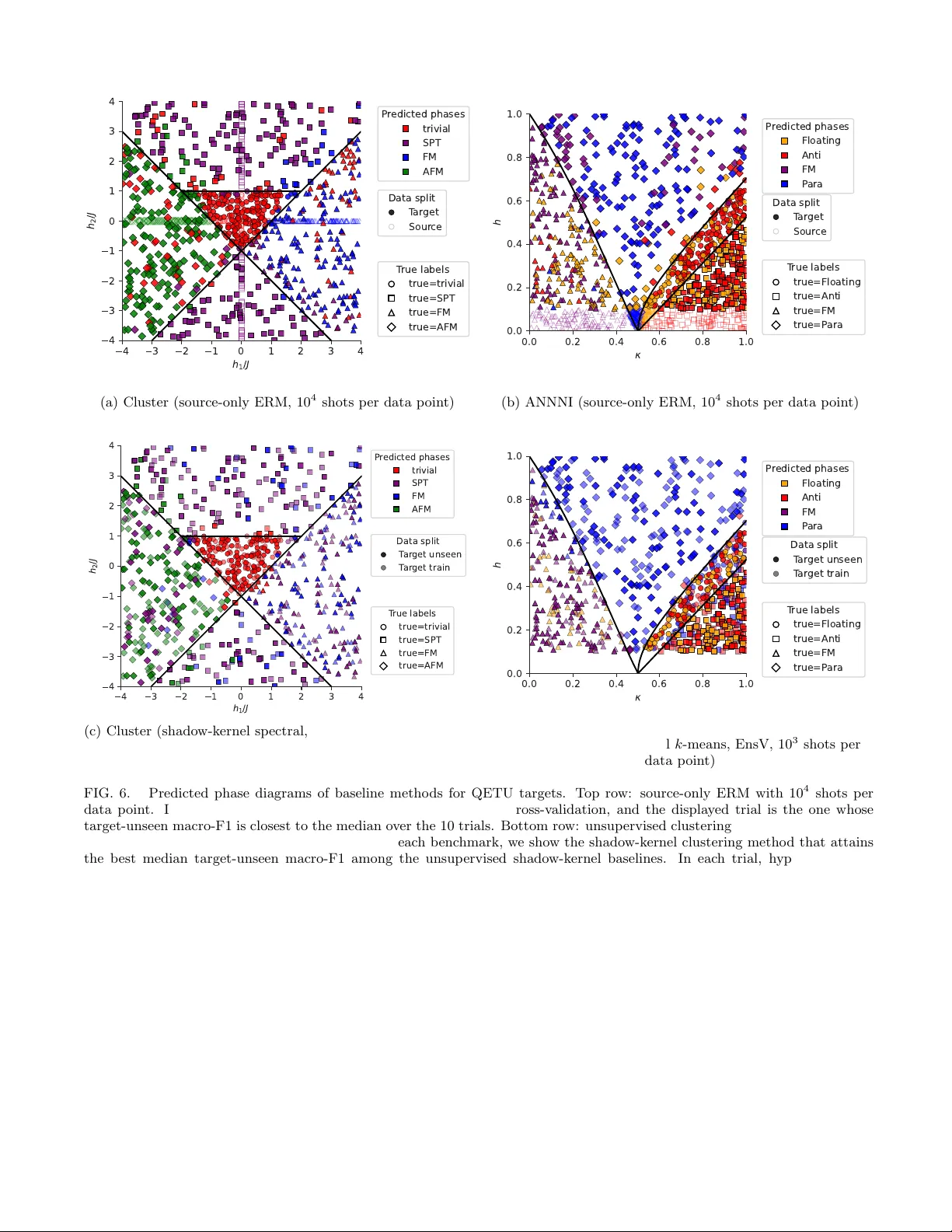
Learning from imp erfect quan tum data via unsup ervised domain adaptation with classical shado ws Kosuk e Ito, 1, 2 , ∗ Akira T anji, 3 Hiroshi Y ano, 2 Y udai Suzuki, 4, 5, 2 and Naoki Y amamoto 2, 3 1 A dvanc e d Material Engine ering Division, T oyota Motor Corp oration, 1200 Mishuku, Susono, Shizuoka 410-1193, Jap an 2 Quantum Computing Center, Keio University, Hiyoshi 3-14-1, Kohoku, Y okohama, Kanagawa 223-8522, Jap an 3 Dep artment of Applie d Physics and Physic o-Informatics, Keio University, Hiyoshi 3-14-1, Kohoku, Y okohama, Kanagawa 223-8522, Jap an 4 Institute of Physics, ´ Ec ole Polyte chnique F´ ed´ er ale de L ausanne (EPFL), L ausanne, Switzerland 5 Centr e for Quantum Scienc e and Engine ering, ´ Ec ole Polyte chnique F´ ed´ er ale de L ausanne (EPFL), L ausanne, Switzerland Learning from quan tum data using classical machine learning models has emerged as a promising paradigm tow ard realizing quantum adv antages. Despite extensiv e analyses on their performance, clean and fully labeled quantum data from the target domain are often una v ailable in practical scenarios, forcing models to be trained on data collected under conditions that diﬀer from those encoun tered at deplo yment. This mismatch highlights the need for new approac hes b eyond the common assumptions of prior work. In this w ork, w e address this issue by employing an unsup ervised domain adaptation framework for learning from imperfect quantum data. Sp eciﬁcally , b y leveraging classical representations of quantum states obtained via classical shado ws, w e p erform unsup ervised domain adaptation en tirely within a classical computational pipeline once measurements on the quan tum states are executed. W e numerically ev aluate the framew ork on quan tum phases of matter and entanglemen t classiﬁcation tasks under realistic domain shifts. Across b oth tasks, our metho d outp erforms source-only non-adaptiv e baselines and target-only unsup ervised learning approaches, demonstrating the practical applicability of domain adaptation to realistic quantum data learning. I. INTR ODUCTION Learning from quantum data with classical machine learning has emerged as a promising route for extract- ing useful information from complex quantum systems including man y-b ody quantum systems. A k ey motiv a- tion b ehind this approach is that the access to quan- tum data changes the computational landscap e of pre- diction tasks, p otentially rendering classically-hard tasks tractable. Recen t theoretical w ork has sho wn that, for suitable problems, learning with quantum data can be eﬃcien t ev en when the corresp onding task without such data is classically in tractable [1–4]. Complemen tary ex- p erimen tal eﬀorts hav e also b egun to supp ort the practi- cal relev ance of this paradigm b y showing that learning can b e p erformed directly on nontrivial quan tum data acquired on quan tum hardware [5, 6]. Among the to ols that make this setting practical, clas- sical shadows provide a compact classical represen tation of quan tum states obtained from randomized measure- men ts, enabling the same measuremen t record to b e reused for many do wnstream estimation tasks without full tomography [7 – 9]. More broadly , recent studies on learning from quantum measurement data include prop- ert y prediction, quantum phase classiﬁcation, adaptive measuremen t-based quan tum state classiﬁcation, learn- ing directly from exp erimen tal quan tum data, shado w- based modeling, and task-agnostic pretraining for quan- tum prop erty estimation [6, 10 – 16]. ∗ kosuk e.ito@quantum.k eio.ac.jp Despite this progress, the assumptions of matched data distributions and abundan t lab els are rarely satisﬁed in realistic applications. In practice, lab eled data are often av ailable only in easier regimes such as numeri- cally tractable parameter regions or w ell-con trolled ex- p erimen ts. By contrast, the target regime is t ypically the one in which reliable lab els are hard to obtain, since cer- tiﬁcation is computationally exp ensiv e or exp erimen tal con trol and characterization are limited, leading to shifts in the underlying parameter distribution. At the same time, the target data are sub ject to v arious sources of noise, including ﬁnite-shot noise, imp erfect state prepa- ration, readout errors and hardware noise [17]. These mismatc hes naturally induce domain shift betw een the data a v ailable for training and the data encountered in the target regime. Although out-of-distribution general- ization has b een established for sp eciﬁc tasks in quantum- pro cess learning and has also b een demonstrated empiri- cally in several man y-b ody state and prop erty prediction tasks [18 – 22], extending learning protocols for quan tum data to broader and more realistic forms of domain shift is an important step to ward robust and practically useful quan tum-data learning. In this work, we address this challenge through un- sup ervise d domain adaptation (UDA) [23–26]. Note that adversarial domain-adaptation ideas hav e previ- ously b een explored for quantum phase classiﬁcation from ground-state data within classical framew ork [27]. Here, we instead study the practically relev ant setting in which lab eled source-domain quan tum data and unla- b eled target-domain quan tum data, represented by clas- sical shadows, are av ailable, with the tw o domains dif- fering in the distribution of observ ed states and, p oten- 2 tially , in the eﬀectiv e relation betw een observed states and lab els. Since classical shadow pro vides classical data ob jects, adaptation and prediction can b e carried out en tirely within a classical computational pip eline once randomized measurements hav e b een p erformed, with- out full state reconstruction or further quantum resources during training. This makes classical shado ws a natural in terface betw een quantum exp erimen ts and UD A. W e ev aluate the prop osed framew ork on t w o repre- sen tative tasks under realistic domain shifts: quan tum phase classiﬁcation [2, 15, 27] and en tanglement classi- ﬁcation [28 – 31]. In the phase-classiﬁcation b enchmarks, the shift arises from mismatched Hamiltonian-parameter regions together with imp erfect ground-state prepara- tion and hardware noise. In the entanglemen t b ench- marks, the shift is induced by diﬀerences in system size, state-generation pro cedures and subsystem parti- tions. Through these experiments, w e sho w that UD A on shado w data improv es predictive p erformance relative to b oth source-only baselines and target-only unsupervised baselines under realistic distribution shifts. These results supp ort UD A as a practical route to ward more robust learning from imperfect quan tum data. The rest of this paper is organized as follows. In Sec. I I, w e formulate the learning problem from the viewp oint of UD A for quan tum data and explain ho w classical shad- o ws naturally yield classical datasets suitable for this set- ting. In Sec. I II, we present the prop osed UDA pip eline for classical-shado w data. In Sec. IV, w e rep ort numeri- cal results on the represen tative learning tasks considered in this work. Finally , Sec. V concludes with a discussion of the main ﬁndings and future directions. Additional n umerical details are provided in the App endix. I I. PR OBLEM SETUP A. Unsup ervised domain adaptation for unlabeled imp erfect quan tum data Let H n := ( C 2 ) ⊗ n b e the n -qubit Hilb ert space and let S ( H n ) denote the set of densit y operators on H n . This work considers the task of predicting a classical la- b el Y ∈ Y from an input quan tum state. T ypical set- tings include classiﬁcation Y = { 1 , 2 , . . . , C } and regres- sion Y = R . Conceptually , the label is assumed to be determined b y an underlying ideal state ρ ideal ∈ S ( H n ) through an unkno wn rule, suc h as a deterministic lab el- ing map ℓ : S ( H n ) → Y satisfying Y = ℓ ( ρ ideal ), or more generally a conditional distribution Q ( Y | ρ ideal ) of the join t input-lab el distribution ( ρ ideal , Y ) ∼ Q . F or ex- ample, the task of classifying quan tum phases of matter considers ρ ideal as a ground state and Y as its phase label (see Sec. IV for details). In realistic situations, ho wev er, the observed states in the target regime typically include errors: ev en when a family of ideal states exists in theory , the actual states ma y b e distorted b y exp erimen tal imperfections, residual coheren t errors, algorithmic imperfections and hardware errors in quan tum devices. As a result, the observ ed state and the label are generically gov erned b y a diﬀerent, unkno wn distribution, ( ρ t , Y t ) ∼ Q t  = Q, (1) where the sup erscripts/subscripts t denote the target data hereafter. Hence, the task in a realistic scenario can b e reduced to estimating the label Y t from the ob- serv ed state ρ t follo wing the unkno wn rule Q t ( Y t | ρ t ). In a simple case, the observ ed state is related to the ideal state as ρ t = E  ρ ideal  , (2) where E is an unknown eﬀectiv e quantum c hannel that characterizes the imp erfections. In this case, the join t distribution of the observ ed state and the lab el is related to the ideal one as Q t (( ρ t , Y t ) ∈ A ) = Q (( ρ ideal , Y ) ∈ T − 1 ( A )) for any even t A ⊂ S ( H n ) × Y , where T ( ρ ideal , y ) := ( E ( ρ ideal ) , y ). In general, since im- p erfection is not necessarily represen ted by a ﬁxed chan- nel E indep endent of the underlying state ρ ideal , we focus on the general target distribution Q t ( ρ t , Y t ). F urthermore, the primary interest often lies in a regime in whic h many quantum states can b e prepared and mea- sured, while reliable lab els are diﬃcult or infeasible to obtain. This diﬃcult y can arise from the aforementioned imp erfections or from the high computational cost for certifying lab els due to classical intractabilit y . This is further exacerbated when the target system is c halleng- ing to con trol and c haracterize or a v ailable quantum- computing resources are insuﬃcien t to generate lab els at scale. Accordingly , learning from unlabeled imp erfect target quan tum data is of signiﬁcan t imp ortance; this is the main motiv ation of our work. More concretely , we assume access to the quantum state ρ t without lab el Y t with underlying distribution ( ρ t , Y t ) ∼ Q t . Although purely unsup ervised learning approac hes based only on the unlabeled target data are also conceiv able [2, 32, 33], they can b e unreliable in the presence of imp erfections. Indeed, as demonstrated in the numerical experiments in Sec. IV, imperfect quan- tum data can substantially degrade the performance of suc h unsupervised baselines. Ev en if lab eled target data are unav ailable, it is of- ten realistic to ha v e access to a related but diﬀeren tly distributed lab eled dataset obtained in a more accessible regime. Examples include regimes in which (i) the quan- tum experiment or quan tum sim ulation is reliable and la- b els can be certiﬁed with mo derate eﬀort, or (ii) classical sim ulation remains tractable and lab els can b e computed. That is, w e hav e access to additional lab eled data with the underlying distribution ( ρ s , Y s ) ∼ Q s  = Q t , whic h we refer to as the source data. Throughout the manuscript, the sup erscripts/subscripts s will denote source data. In addition to diﬀerences in the resp ective state’s marginal distributions Q s ρ and Q t ρ of the source and the target do- mains across the accessible regimes, imp erfections in the 3 Source domain ( ρ s , Y s ) ∼ Q s T arget domain ρ t ∼ Q t ρ UD A FIG. 1. Schematic illustration of unsup ervised domain adap- tation (UD A) for quantum data. (Upp er) The labeled source domain and the unlab eled target domain follow diﬀerent dis- tributions; as a consequence, the decision b oundary learned on the source domain is generally misaligned with the target data. (Lo wer) A feature-extraction map is learned so that the resulting representation preserv es lab el-relev ant structure while reducing domain-speciﬁc discrepancies, enabling a de- cision rule that transfers from the source to the target do- main. One such method is a domain-adv ersarial training as describ ed in Sec. I I I. target data-generation pro cess can alter the relation be- t ween an observed state and the underlying ideal state that determines the label. Consequen tly , even when the same observed state ρ app ears in b oth domains, the con- ditional distribution can diﬀer, Q t ( Y | ρ )  = Q s ( Y | ρ ). F or example, if ρ t = E ( ρ ideal ) while ρ s = ρ ideal , then the same observ ed ρ can originate from diﬀeren t ideal states across domains. The ab ov e setting, where a predictor is learned to p er- form w ell on the unlabeled target domain by exploiting lab eled data from a related but diﬀeren t source domain, is kno wn in machine learning as unsup ervise d domain adaptation (UDA) [23–26]. In UD A, each data domain of source/target data is called source/target domain. Fig. 1 sc hematically summarizes this setting. In the original state space, the source and target domains can exhibit a substantial distribution mismatch, so that a predictor trained only on labeled source data ma y fail to general- ize to the target domain. UD A addresses this issue by learning a feature representation in which label-relev an t structure is retained while domain-sp eciﬁc v ariation is suppressed, thereb y improving transfer to unlab eled tar- get data. In particular, the presen t UDA setting is not restricted to the so-called cov ariate-shift Q s ρ  = Q t ρ under Q t ( Y | ρ ) = Q s ( Y | ρ ), but it also allows for the concept shift Q t ( Y | ρ )  = Q s ( Y | ρ ) [34]. B. Classical dataset consisting of classical shado ws A practically relev ant setting restricts the access of classical learning mo dels to classical information ob- tained from quan tum input states. In particular, the setup do es not assume full access to the quantum state ρ suc h as p erforming tomography . Instead, each quan tum state is measured locally to pro duce partial classical data, and then a classical learning algorithm is applied to the resulting classical datasets. This framework is motiv ated by practical constraints. Main taining a large collection of quantum states as a rep eatedly accessible database would require quantum memory at scale, and end-to-end quan tum learning mod- els require coherent access to quantum data and nontriv- ial exp erimental ov erhead. By contrast, storing classical information extracted from quan tum states is compati- ble with current and near-term experimental w orkﬂows and oﬀers an additional practical beneﬁt: once a clas- sical database is constructed, the same records can b e reused for m ultiple downstream purp oses, including esti- mating many diﬀerent target properties ev en after data acquisition [7, 35, 36]. While the learning stage remains classical, a p otential quan tum adv antage or a practical quan tum utilit y can still b e exp ected when constructing the classical dataset from quan tum data is prohibitiv e for purely classical metho ds. This exp ectation stems from the fact that some tasks are classically eﬃcient with the aid of quantum data while classically hard without data [1, 3, 4, 37]. Suc h a regime ma y also arise even when the av ailable quan tum data are mo derately imp erfect. Realizing this p otential adv an tage in the actual learning task, how ev er, still requires eﬀectiv e metho ds that can exploit suc h data. The fo cus of this w ork is to pro vide suc h a metho d within the UDA framework. Among several measurement proto cols, a particularly simple and exp erimentally feasible option is the P auli classical shadow [7], where single-qubit random Pauli measuremen ts are performed to eﬃciently store classical snapshots of quantum data. Although Cliﬀord classical shado ws [7] or entangled measuremen ts across m ultiple copies of the state [5, 38] oﬀer stronger theoretical guar- an tees, this work adopts Pauli classical shadows as the data-extraction metho d due to their ease of implementa- tion and compatibility with near-term exp erimental plat- forms. The proto col pro ceeds as follows. Giv en an n -qubit state ρ , T indep endent measurement shots are collected. In P auli classical shadow [7], a random measurement set- ting is c hosen for eac h shot j ∈ { 1 , . . . , T } : P j = ( P 1 ,j , . . . , P n,j ) ∈ { X, Y , Z } n . (3) Eac h qubit lab eled i is then measured in the eigenbasis of P i,j , and the corresp onding outcome bit b i,j ∈ { 0 , 1 } 4 ρ s i ρ t j Shado w meas. Shado w meas. Source domain quantum data T arget domain quantum data ( S T s ( ρ s i ) , y s ) S T t ( ρ t j ) z ˜ z Φ s Φ t F eatures computed from classical shadows − λ ∇ θ f L dom ∇ θ f L Y ∇ θ Y L Y − λ ∇ θ Y L dom ∇ θ dom L dom CNN F eature extractor G θ f h DSBN BN s BN t A s w s A t w t Lab el classiﬁer Domain discriminator D θ dom C θ Y Lab el prediction ˆ y Domain prediction ˆ d Loss L Y Loss L dom GRL FIG. 2. Learning pipeline for unsup ervised domain adaptation from classical shado w datasets based on CDAN. The input is the labeled source data ( S T s ( ρ s i ) , y ) ∈ D s N s or the unlabeled target data S T s ( ρ s j ) ∈ D t N t , eac h consisting of P auli classical shado w. A feature map Φ d con verts eac h shadow record to an input feature tensor z whose size may dep end on the domain d . The feature extractor G θ f consists of an input-size adapter A d w d to conv ert z to a ﬁxed-shap e input ˜ z follow ed by a CNN that tak es ˜ z as input. The CNN includes DSBN lay ers BN d . The latent feature h = G θ f ( z ) is con verted to the label probability distribution via a lab el classiﬁer C θ Y to give a lab el prediction ˆ y by taking the argmax. The Kronec ker pro duct of h and the lab el probability distribution is fed into a domain discriminator D θ dom , which outputs a prediction of which domain the given data b elongs to. While the feature extractor and the lab el classiﬁer are trained to minimize the label classiﬁcation loss L Y using lab eled source examples, they are sim ultaneously trained to maximize the domain discrimination loss L dom via GRL. The domain discriminator is adversarially trained to minimize L dom . This w a y , the lab el-conditional latent feature distributions o ver the tw o domains are made similar while keeping the class-lab el distinguishability . is recorded. The eigenstate of eac h qubit after measure- men t in the chosen setting can b e represented as | s i,j ⟩ ∈ {| 0 ⟩ , | 1 ⟩ , | + ⟩ , |−⟩ , | i+ ⟩ , | i −⟩} , (4) where | 0 ⟩ , | 1 ⟩ are Z -eigenstates, |±⟩ are X -eigenstates, and | i ±⟩ are Y -eigenstates. Hence, the classical snapshot of j -th shot with the measurement setting P j can b e enco ded as the pro duct state as | s j ⟩ := N n i =1 | s i,j ⟩ . W e denote the resulting classical shadow data b y S T ( ρ ) :=  ( P j , b j )  T j =1 ≡  | s i,j ⟩ : i ∈ { 1 , . . . , n } , j ∈ { 1 , . . . , T }  , (5) where b j := ( b 1 ,j , . . . , b n,j ). The key p oin t is that S T ( ρ ) is a purely classical ob ject that can b e stored and reused. Moreo ver, by p ost-pro cessing the classical snap- shots, man y diﬀerent properties of ρ can b e estimated from the same shadow dataset, without reconstructing ρ itself. Within this setup, our goal is hence summarized as classical learning of the prediction rule Q t ( Y t | ρ t ) from the unlab eled target-domain classical data D t N t :=  S T t ( ρ t j )  N t j =1 , ρ t j i . i . d . ∼ Q t ρ , (6) with the aid of the lab eled source-domain classical data D s N s :=  ( S T s ( ρ s i ) , y s i )  N s i =1 , ( ρ s i , y s i ) i . i . d . ∼ Q s , (7) where, in general, the joint distributions diﬀer, ( ρ s , Y s ) ∼ Q s , ( ρ t , Y t ) ∼ Q t , Q s  = Q t . Accordingly , this work adopts the UDA viewp oin t to address learning from unlab eled P auli classical shado ws of imperfect quantum data. The next section speciﬁes ho w classical-shadow-deriv ed features are constructed and ho w UD A ob jectiv es are instantiated in the learn- ing pip eline. I II. UNSUPER VISED DOMAIN AD APT A TION METHODS F OR CLASSICAL SHADOW D A T ASET This section presen ts the learning methods for UD A using Pauli classical shado w datasets. F or concreteness, w e form ulate the pip eline focusing on the classiﬁcation tasks, although it can b e generalized to the regression. W e ﬁrst introduce the ov erall pip eline of the metho d and then describe its main comp onen ts in detail. Since target lab els are unav ailable in UDA, we also introduce a lab el- free mo del-selection strategy for h yp erparameter tuning later in Sec. I I I E. 5 A. Whole pip eline Fig. 2 summarizes the whole pip eline with ov erall data ﬂow. The classical shado w of eac h quantum data is used to extract an input feature tensor. This fea- ture tensor is pro cessed b y a neural feature extractor trained join tly with a label classiﬁer and a domain dis- criminator within the conditional domain adversarial net- w ork (CDAN) framework [39]. The adversarial ob jectiv e promotes representations that remain discriminative for the prediction task while remaining approximately in- v ariant to domain shifts betw een the source and target datasets. More concretely , given a classical shado w record S T d ( ρ d ) from eac h domain d ∈ { s , t } , w e ﬁrst compute a feature tensor z = Φ d ( S T d ( ρ d )) by applying a classical p ost-processing map Φ d as detailed in Sec. I II B. Here, the map Φ d ma y b e domain dep enden t in general if each domain has distinct size of the underlying quan tum sys- tem. A domain-dep endent input-size adapter A d w d is then applied to obtain ˜ z = A d w d z to resolve the size diﬀerence if needed (see Sec. I II C). The resulting representation is subsequently pro cessed b y a conv olutional neural net- w ork (CNN) e G d θ d CNN to pro duce the laten t embedding, whose dep endence on d comes from the domain-sp eciﬁc batc h normalization (DSBN) [40] la yers of CNN. As de- scrib ed in Sec. I II C, each batch normalization lay er BN is replaced by a domain speciﬁc one BN d to accommo- date for the statistical diﬀerence betw een the domains. The resulting feature extractor G d θ f reads h = G d θ f ( z ) = e G d θ d CNN ( A d w d z ) , where θ f denotes the whole trainable parameters of the feature extractor including the input-size adapters and CNNs for both domains. The lab el classiﬁer C θ Y consists of a single linear la yer with trainable param ters θ Y and the softmax lay er to output class probabilit y distribution ( p θ f , θ Y ( y | z )) y = C θ Y ( h ) . The lab el loss L Y is ev aluated only on the lab eled source examples. In CDAN, the input u = vec  h ⊗ p θ f , θ Y ( ·| z )  is fed into the domain discriminator D θ dom , where ⊗ de- notes the Kroneck er pro duct and θ dom denotes the train- able parameters. The discriminator also consists of a single linear lay er and the softmax la yer to output the probabilit y q θ f , θ Y , θ dom ( d | z ) = ( D θ dom ( u ) ( d = s) 1 − D θ dom ( u ) ( d = t) . The discriminator is trained on both source and target examples so that the head param ters θ dom are updated to decrease the domain loss L dom , while the feature ex- tractor G d θ f is up dated to increase the domain loss L dom via the gradien t rev ersal la yer (GRL) as describ ed in Sec. I I I D. The resulting forward mapping is depicted in Fig. 3. S T s / t ( ρ s / t ) Φ s / t − − − − → z G s / t θ f − − − − → h C θ Y − − − − → p θ f , θ Y ( ·| z ) argmax − − − − − − → ˆ y , v ec  h ⊗ p θ f , θ Y ( ·| z )  argmax ◦ D θ dom − − − − − − − − − − − → ˆ d , FIG. 3. The forward mapping of the whole pip eline. B. Input feature tensor from classical shado ws Eac h classical shado w record S T ( ρ ) is ﬁrst mapp ed in to an input represen tation z for the do wnstream neu- ral netw ork. Classical shado ws pro vide sample-eﬃcient estimates of exp ectation v alues for a large set of lo cal observ ables through classical p ost-processing. Accord- ingly , the representation z can b e regarded as an input feature tensor constructed from estimated local observ- ables, where the sp eciﬁc c hoice of observ ables is guided b y the learning task and the structural properties of the underlying quantum data. More sp eciﬁcally , let { O α } α b e a collection of observ- ables. F rom S T ( ρ ), we can compute estimators [ ⟨ O α ⟩ ρ for ⟨ O α ⟩ ρ := T r[ O α ρ ]. Then, we deﬁne a feature map z = Φ d ( S T d ( ρ d )) :=  [ ⟨ O d α ⟩ ρ  α with eac h observ able set { O d α } α for domain d. Those observ ables should b e chosen so that z captures label- relev ant information while remaining feasible to estimate with the a v ailable n umber of shots T d . In particular, for quantum data whose system is de- ﬁned on a lattice, it is natural to organize the fea- tures as a tensor aligned with the lattice [2]. Let Λ = { 1 , ..., L 1 } ⊗ · · · ⊗ { 1 , ..., L D } denote the D -dimensional lattice of size L 1 × · · · × L D , and write each site as i ∈ Λ. F or simplicity , w e fo cus on features constructed from t wo- site reduced densit y matrices. The extension to general r -site reduced density matrices is straightforw ard. F or eac h site i ∈ Λ, choose an ordered subset Λ i = { j (1) i , . . . , j ( M ) i } ⊂ Λ \{ i } . W e assume that | Λ i | = K or 0 with a ﬁxed n umber K . F or example, for a 1D lattice Λ = { 1 , . . . , L } with the open b oundary condition, one ma y tak e up to the k -nearest-neighbor sites Λ ( k ) i = ( { i + 1 , . . . , i + k } ( i = 1 , . . . , L − k ) ∅ ( i = L − k + 1 , . . . , L ) , (8) where K = k holds in this case. F or each single-qubit P auli op erator P ∈ { I , X , Y , Z } , let P i denote the | Λ | -qubit operator with weigh t one that 6 acts as P on site i and as the iden tity on ev ery other site. W e also ﬁx an ordering { ( P , Q ) ∈ { I , X , Y , Z } 2 : ( P , Q )  = ( I , I ) } = { ( P ( a ) , Q ( a ) ) } 15 a =1 . (9) Then, for eac h pair ( i , j ) with j ∈ Λ i , we estimate the 15 nontrivial tw o-site P auli exp ectation v alues ˆ c ( a ) i , j := \ ⟨ P ( a ) i Q ( a ) j ⟩ ρ , a = 1 , . . . , 15 . (10) These co eﬃcien ts completely c haracterizes the t wo-site reduced density matrix of sites i , j through its P auli- basis expansion. F or eac h i and m = 1 , . . . , K , deﬁne the 15-dimensional vector ˆ c ( m ) i :=  ˆ c (1) i , j ( m ) i , . . . , ˆ c (15) i , j ( m ) i  ⊤ ∈ R 15 . (11) W e then deﬁne the feature v ector at site i b y concate- nating these v ectors ov er all j ∈ Λ i : z i :=  ( ˆ c (1) i ) ⊤ , . . . , ( ˆ c ( M ) i ) ⊤  ⊤ ∈ R 15 M . (12) Equiv alently , the feature tensor entries can b e written explicitly as z i , l := ˆ c ( a ) i , j ( m ) i ( l = 15( m − 1) + a, m = 1 , . . . , K , a = 1 , . . . , 15) . (13) Th us, the full feature tensor is z = ( z i ,l ) ∈ R L 1 ×···× L D × 15 K . (14) This tensor can b e fed directly into a D -dimensional CNN, with i treated as the spatial index and l as the input-c hannel index. W e can also fed the feature ten- sor z to one-dimensional CNN b y vectorizing i . This represen tation allows the CNN to learn nonlinear func- tions of lo cal reduced states inv olving correlations cap- tured b y Λ i . Especially , for D = 1 with Λ ( k ) i deﬁned b y Eq. (8), w e denote the resulting feature map S T ( ρ ) 7→ z b y Φ 1 k , whic h can tak e into accoun t correlations up to k -nearest-neigh b or. In our numerics for one dimensional systems in Sec. IV A, we use this family of lo cal reduced- densit y feature maps with an appropriate choice of k for eac h task. C. Domain-sp eciﬁc batc h normalization and input-size adapter Our CNN feature extractor contains batch normaliza- tion (BN) lay ers, which normalize in termediate activ a- tions using batc h statistics and learned aﬃne parame- ters. In UD A, sharing BN lay ers across domains can b e sub optimal b ecause activ ation statistics can diﬀer sub- stan tially betw een the source and target domains. T o accoun t for this, we employ DSBN [40], which maintains separate BN parameters and running statistics for the source and target domains. Concretely , eac h BN lay er is replaced by a pair BN s and BN t with indep endent aﬃne parameters and running momen ts, and the appropriate branc h is selected according to the domain of each input. The remaining con volutional weigh ts are shared. In addition, some datasets inv olv e diﬀerent input di- mensions across domains, for example, due to diﬀeren t feature constructions or diﬀerent num b ers of lo cal ob- serv ables. T o handle this setting within a uniﬁed arc hi- tecture, we in tro duce a trainable linear input-size adapter A s / t w s / t that maps eac h domain input in to a common di- mension: ˜ z = ( A s w s z , ( z from the source domain) , A t w t z , ( z from the target domain) , where ˜ z has a ﬁxed dimension shared b y b oth domains. When the source and target inputs already hav e the same dimension, we set A s w s = A t w t = I and omit this adapter. Fig. 2 includes this input-adaptation stage as an explicit comp onen t when needed. With DSBN and input-size adapter, the feature extrac- tor b ecomes domain conditioned. One ma y decomp ose θ f in to shared CNN parameters θ sh CNN and the domain- sp eciﬁc parts as θ f = ( θ sh CNN , θ BN s CNN , θ BN t CNN , w s , w t ). F or brevit y , w e use the shorthand G s / t θ f for the feature ex- tractor and do not expand domain-dependent parameters explicitly in the subsequent notation. D. Conditional domain adv ersarial netw ork W e next describ e the details of CD AN. In the original domain-adv ersarial neural netw ork (DANN) formulation for UD A [24], the discriminator directly takes the la- ten t feature h as input, thereby encouraging alignmen t of the latent marginal distributions of b oth domains. How- ev er, such marginal alignment can b e insuﬃcien t when the data distribution has complex m ulti-mo dal struc- tures [39]. CD AN w as in ven ted to address this issue b y conditioning the discriminator on the predicted class probabilities [39]. Concretely , CD AN feeds u = v ec  h ⊗ p θ f , θ Y ( ·| z )  , in to the discriminator D θ dom to take into accoun t the lab el-conditional latent distribution. F urthermore, we emplo y the en trop y conditioning to suppress the con tri- bution of uncertain predictions. The uncertaint y of a probabilit y distribution ( p ( y )) y is quantiﬁed b y the en- trop y H ( p ) = − P y p ( y ) log p ( y ), and the en tropy-a ware w eight w ( z ) = 1 + e − H ( p θ f , θ Y ( ·| z )) is applied. Hence, the 7 domain loss is deﬁned as L dom ( θ f , θ Y , θ dom ) = E ρ s ∼ Q s ρ h − w ( z s ) log D θ dom  u s  i + E ρ t ∼ Q t ρ h − w ( z t ) log  1 − D θ dom  u t  i , (15) while the lab el loss L Y is computed only on lab eled source examples: L Y ( θ f , θ Y ) = E ( ρ s ,y s ) ∼ Q s h − log p θ f , θ Y  y = y s | z  i . The o v erall training ob jective follows the standard ad- v ersarial formulation, where the discriminator minimizes L dom , while the feature extractor and the lab el classiﬁer minimize L Y and sim ultaneously confuse the discrim- inator. With a trade-oﬀ hyperparameter λ > 0 and L ( θ f , θ Y , θ dom ) := L Y ( θ f , θ Y ) − λ L dom ( θ f , θ Y , θ dom ), this corresp onds to the minimax problem min ( θ f , θ Y ) L ( θ f , θ Y , θ dom ) , (16) max θ dom L ( θ f , θ Y , θ dom ) . (17) In practice, this is implemen ted b y the bac kpropagation with a GRL inserted b et ween the discriminator and the rest of the netw ork. W riting the updates in a sto c hastic gradien t descen t (SGD) form with learning rate η > 0 using mini-batch estimates b L Y , b L dom , we hav e θ dom ← θ dom − η ∇ θ dom b L dom , (18) θ f ← θ f − η  ∇ θ f b L Y − λ ∇ θ f b L dom  , (19) θ Y ← θ Y − η ( ∇ θ Y b L Y − λ ∇ θ Y b L dom  . (20) E. Mo del selection without target labels Hyp erparameter tuning and ep o c h selection are non- trivial in the UDA setting, since target labels are una v ail- able and standard cross-v alidation on the target domain cannot be applied. Consequen tly , mo del selection m ust rely on lab el-free signals computable from unlab eled tar- get data, p ossibly together with lab eled source data. A v ariety of such criteria ha v e been prop osed in the litera- ture, including source domain-based metho ds [24, 41 – 43] and target domain-based methods [44 – 47]. Among these, w e employ tw o of the target domain-based metho ds b e- lo w. W e proceed as follows. F or each candidate h yp er- parameter conﬁguration, w e train a CD AN mo del us- ing labeled source data and unlab eled target data. Let M 1 , . . . , M K denote the resulting trained mo dels. F or eac h model M m and each unlab eled target example z t , w e compute the output lab el prediction probabilit y dis- tribution p M m ( y | z t ). W e then ev aluate the follo wing lab el-free criteria on the target domain data: • InfoMax [45, 47]. Information Maximization (In- foMax) uses input-output mutual information max- imization as a matric [45, 47, 48]. InfoMax bal- ances lo w conditional entrop y on individual target examples with high marginal entrop y of the av erage prediction, which discourages degenerate solutions that collapse all predictions to a single class. Con- cretely , deﬁne the target predictiv e entrop y H tgt ( M m ) = E ρ t ∼ Q t ρ  H  p M m ( ·| z t )  , and the marginal entrop y of the av erage prediction H  E ρ t ∼ Q t ρ [ p M m ( ·| z t )]  . The InfoMax score is then an empirical estimation of I tgt ( M m ) = H  E ρ t ∼ Q t ρ [ p M m ( ·| z t )]  − H tgt ( M m ) , and mo dels with larger v alues of I tgt ( M m ) are pre- ferred. • EnsV [47]. Ensemble-based V alidation (EnsV) se- lects a mo del that best agrees with the consensus b eha vior across candidate mo dels on the unlab eled target data [47]. In EnsV, w e treat the ensem ble- a verage prediction ¯ p ( y | z t ) = 1 M M X m =1 p M m ( y | z t ) as a virtual teac her and select the mo del with the largest agreement with ¯ p . Intuitiv ely , this fav ors mo dels that match the stable predictions shared across conﬁgurations, while reducing sensitivit y to idiosyncratic behaviors of any single run. W e can use an arbitrary quan tiﬁcation of the agreemen t be- t ween each candidate mo del and ¯ p dep ending on the purp ose. A simple implemen tation uses the a verage inner pro duct A ( M m ) = E ρ ∼ Q t ρ  ⟨ p M m ( ·| z t ) , ¯ p ( ·| z t ) ⟩  . F or classiﬁcations, we can use a classiﬁcation score metric such as macro-F1 score regarding ¯ p as the ground truth, as we do in the n umerics in Sec. IV. IV. NUMERICAL RESUL TS This section ev aluates the UD A pip eline introduced in Sec. I II on t wo quan tum-data classiﬁcation tasks: clas- siﬁcation of quantum phases of matter and classiﬁcation of entangled states. W e brieﬂy describe the common settings used in the follo wing numerical exp erimen ts. W e ﬁrst generate the underlying quantum states b y randomly sampling N s = 400 labeled source samples and N t = 800 unlab eled 8 target samples, with the n umbers of samples balanced across classes, and then keep these quan tum states ﬁxed throughout 10 trials. In each trial, the target samples are randomly split ev enly in to t wo subsets: 400 samples are used as unlab eled target-train data for adaptation, and the remaining 400 samples are held out as unseen target data for score ev aluation. Th us, the subset of target sam- ples used for adaptation v aries across trials. In eac h trial, the en tire pip eline is executed end-to-end, including (i) generating classical-shadow measuremen t data, (ii) con- structing shado w-based classical features, (iii) training mo dels, and (iv) selecting a mo del without target lab els using the methods in Sec. II I E. The rep orted p erformance metrics are the median, the mean and standard deviation of the macro-F1 score of the unseen target data o v er these 10 trials. In our n u- merics, w e use a one-dimensional CNN with DSBN for the feature extractor, and linear heads for both class pre- diction and domain discrimination in the UDA pip eline sp eciﬁed in Sec. I I I. The detailed implemen tation is given in App endix A. W e use the Adam optimizer [49] to train the mo dels. The hyperparameter grids are E ∈ { 200 , 300 , 400 , 500 , 600 , 700 , 800 , 900 , 1 , 000 } , B ∈ { 20 , 50 , 80 } , η ∈ { 10 − 6 , 5 × 10 − 6 , 10 − 5 , 5 × 10 − 5 , 10 − 4 } , (21) where E , B and η are the n umber of epo chs, the mini- batc h size, and the learning rate, resp ectively . F or CD AN, the domain-loss w eight λ is additionally swept o ver λ ∈ { 0 . 5 , 1 . 0 , 1 . 5 } . (22) The target-domain quantum data include state- preparation imp erfections, while the source-domain quan tum data are taken to b e clean. State-preparation imp erfections are in troduced in a task-dependent manner and are speciﬁed for each task. W e compare the UDA metho d with the following tw o baselines that do not p erform domain adaptation: (i) Sour c e-only empiric al risk minimization (ERM). This baseline corresp onds to training the same CNN feature extractor and a linear classiﬁer only on labeled source data, and then applying the re- sulting mo del to the target data without adapta- tion. F or mo del selection, w e use cross-v alidation on the source domain. More precisely , for each hy- p erparameter conﬁguration and candidate num b er of epo chs in (21), w e select the b est setting using three-fold cross-v alidation on the source dataset, and then reﬁt the mo del on the full source data with a selected hyperparameter (ii) Unsup ervise d le arning on the tar get via the shadow kernel. A natural lab el-free approac h is to apply unsup ervised learning directly to the target shad- o ws by using a similarit y meas ure betw een classical shado ws. W e use the shadow kernel [2] k sh  S T t ( ρ t j ) , S T t ( ρ t j ′ )  := exp   τ T 2 t T t X l,l ′ =1 exp   γ n n X j,j ′ =1 T r( σ j,l σ j ′ ,l ′ )     , (23) where σ j,l := 3 | s j,l ⟩ ⟨ s j,l | − I , and construct the tar- get Gram matrix K t j j ′ := k sh  S T ( ρ t j ) , S T ( ρ t j ′ )  ∈ R N t × N t . (24) W e then run kernel-based clustering (k ernel k - means and spectral clustering) on K t . The kernel h yp erparameters are sw ept ov er τ ∈ { 0 . 01 , 0 . 1 , 1 . 0 , 3 . 0 } , γ ∈ { 0 . 01 , 0 . 1 , 1 . 0 } . (25) Although lab el information is not a v ailable within the unsupervised learning, cluster indices are re- ordered after training using the hidden target la- b els to maximize the score for comparison with the UD A metho d. Of course, the target lab els are never used in the training or mo del selection. A. Classiﬁcation of quan tum phase of matter In this subsection, we consider phase classiﬁcation tasks on quantum many-bo dy datasets of 1D cluster mo del, 1D axial next-nearest-neighbor Ising (ANNNI) mo del [50], toric co del [51] and color co de [52] systems. Eac h data p oin t is asso ciated with the ground state of a Hamiltonian of the system. Although we conduct the classiﬁcation on the data of ﬁnite-size systems, the task is to predict the quantum phase of the corresponding ground state deﬁned in the thermo dynamic limit. In this task, domain adaptation is motiv ated b y the practical discrepancy b et w een lab eled data and the data of interest at deplo yment. Lab eled source data are typi- cally a v ailable in regimes where the Hamiltonian is easier to sim ulate or the states are easier to prepare, whereas the target regime can b e harder b oth to prepare accu- rately and to lab el b y an accurate computation. More- o ver, the target data can diﬀer from the source data not only because the Hamiltonian parameters are distributed diﬀeren tly , but also b ecause the prepared states are only appro ximate ground states and are further aﬀected by hardw are noise suc h as depolarizing errors. Therefore, ev en when the target task is the same phase classiﬁca- tion problem, a mo del trained only on lab eled source data need not generalize well to the unlab eled target do- main, making unsup ervised domain adaptation a natural framew ork in our setting. 9 4 3 2 1 0 1 2 3 4 h 1 / J 4 3 2 1 0 1 2 3 4 h 2 / J 0.0 0.2 0.4 0.6 0.8 1.0 F idelity (a) Cluster mo del 0.0 0.2 0.4 0.6 0.8 1.0 0.0 0.2 0.4 0.6 0.8 1.0 h 0.0 0.2 0.4 0.6 0.8 1.0 F idelity (b) ANNNI mo del FIG. 4. Ground-state subspace ov erlap of the target domains for (a) Cluster and (b) ANNNI mo dels with QETU-based algo- rithmic state-preparation imp erfection. Each panel shows F G ( x ) = ⟨ ψ | Π G ( x ) | ψ ⟩ at the corresp onding Hamiltonian parameters. Only target domains are shown b ecause source states are exact in these simulations. 1. Cluster Hamiltonian The Cluster Hamiltonian is deﬁned as H = n X j =1  J Z j − h 1 X j X j +1 − h 2 X j − 1 Z j X j +1  , (26) whic h supp orts m ultiple phases including a symmetry- protected topological (SPT), trivial, ferromagnetic, and an ti-ferromagnetic phases dep ending on the parameters x = ( h 1 /J, h 2 /J ). W e consider a system of n = 15 spins. In this mo del, we use the input feature map Φ 1 k with k = 1 deﬁned in Sec. I II B as a minimal choice. a. Err or mo dels. W e mo del algorithmic imp erfec- tions by replacing the ideal ground state with a sup erp o- sition of lo w-energy eigenstates. Let G ( x ) ⊂ H n denote the low-energy subspace that w e use as the ground-state subspace at parameter x , and let Π G ( x ) b e the pro jector on to it. Since all phases of this mo del are gapp ed phases, G ( x ) is taken as the span of the low est d 0 eigenstates, where d 0 matc hes the degen- eracy of the ground states in the thermo dynamic limit. Concretely , we use d 0 = 4 in the SPT phase, d 0 = 2 in the ferromagnetic and the anti-ferromagnetic phases, and d 0 = 1 in the trivial phase. Then, we quantify the al- gorithmic imperfection in the preparation of the ground state | ψ ⟩ at the parameter x by its ov erlap with the sub- space G ( x ) F G ( x ) = ⟨ ψ | Π G ( x ) | ψ ⟩ . F or each Hamiltonian parameter x , we compute the low- est N exc + 1 eigenpairs with N exc = 40 using sparse exact diagonalization based on the implicitly restarted Lanczos metho d via SciPy [53, 54]. Sp eciﬁcally , w e mo del a tw o-stage imp erfect state- preparation pip eline and consider t wo target-state con- structions obtained by truncating this pipeline at diﬀer- en t stages. • The ﬁrst construction mo dels the output of the ini- tial preparation stage b efore any subsequent spec- tral ﬁltering. W e therefore denote the state by | ψ raw ( x ) ⟩ , where “raw” indicates the ra w output of the initial state preparation routine. Namely , w e use this model to represen t a generic output of appro ximate ground-state preparation routines that only partially reach the desired lo w-energy sec- tor. F or instance, near-term ground-state prepa- ration algorithms such as the v ariational quan- tum eigensolver, quan tum imaginary time ev olu- tion, and adiabatic state preparation [55 – 57] may pro duce such states. In suc h settings, ﬁnite circuit depth, imp erfect optimization, or limited evolution time can lea ve non-negligible excited-state contami- nation. T o model this scenario, the ﬁdelity parame- ter f is drawn uniformly from the in terv al [0 . 2 , 0 . 4]; then, the states | v g ⟩ and | v e ⟩ are uniformly sampled from G ( x ) and its orthogonal complemen t within the span of the computed eigenv ectors, resp ectively . Concretely , the raw target state is deﬁned as | ψ raw ( x ) ⟩ = p f | v g ⟩ + p 1 − f | v e ⟩ . • The second construction extends the same pip eline to the early fault-tolerant regime, where more ad- v anced quantum algorithms b ecome accessible. As a representativ e example, we consider a sp ectral ﬁltering step tailored to this setting. Given an ini- tial state with nonzero ov erlap with the ground or 10 lo w-energy subspace, such metho ds suppress high- energy comp onents while amplifying the desired o verlap [58, 59]. Accordingly , this construction rep- resen ts the same imp erfect initial preparation fol- lo wed by an additional ﬁltering stage, and therefore t ypically yields a higher ov erlap with G ( x ) than the ra w state in the ﬁrst mo del. In particular, we apply the QETU-based sp ec- tral ﬁlter prop osed in Ref. [59] to the input state | ψ raw ( x ) ⟩ . W e use a ﬁlter P k deg  cos  ˜ H ( x ) / 2  constructed from ev en Chebyshev p olynomials of up to degree k deg = 40, where ˜ H ( x ) is an aﬃne- transformed Hamiltonian whose sp ectrum is con- tained in [ η , π − η ] with η = 0 . 05. The resulting target state is | ψ QETU ( x ) ⟩ = P k deg  cos  ˜ H ( x ) / 2  | ψ raw ( x ) ⟩    P k deg  cos  ˜ H ( x ) / 2  | ψ raw ( x ) ⟩    . In the generation of n umerical data, we do not sim- ulate the QETU circuit itself. Instead, the induced sp ectral ﬁlter is directly applied to the computed eigenstates. F or the p olynomial P k deg , we need an estimate of the spectral gap [59] and hence use a ﬁxed gap estimate ∆ est = 1 for all x . F urther de- tails of b oth target constructions are given in Ap- p endix B. Fig. 4(a) sho ws the resulting target-state o verlap F G ( x ) with the subspace G ( x ). After either algorithmic imp erfection is applied, hardw are-type noise is included by applying single-qubit dep olarizing noise and measuremen t bit-ﬂip noise with rates p depol = 0 . 1 and p ﬂip = 0 . 01. b. Domain shift. In the source domain, the Hamil- tonian parameters are sampled from R s := { ( h 1 /J, 0) | − 4 ≤ h 1 /J ≤ 4 } ∪ { (0 , h 2 /J ) | − 4 ≤ h 2 /J ≤ 4 } , where the source region is chosen as the union of tw o ex- actly solv able lines [60, 61]. The features are computed from exact exp ectation v alues of the clean ground states without any error, corresponding to exact sim ulation or to the limit T s → ∞ . In fact, when the source states are classically simulable, exact computation of the exp ecta- tion v alues can be easier than sampling. W e denote the resulting source dataset by R s -Exact- ∞ . The target-domain parameters are sampled from R t = { ( h 1 /J, h 2 /J ) | − 4 ≤ h 1 /J, h 2 /J ≤ 4 }\ R s , whic h induces a distribution shift in the Hamiltonian pa- rameters. Moreo ver, the target states are generated b y the t wo-stage imp erfect state-preparation pip eline abov e. That is, we either stop at the ra w preparation stage and use | ψ raw ( x ) ⟩ , or we further apply the QETU ﬁl- ter to obtain | ψ QETU ( x ) ⟩ . In both cases, the resulting states are sub ject to hardw are-t yp e noise as describ ed in Sec. IV A 1 a. The target features are then computed from Pauli classical shadows with T t = 10 3 or 10 4 shots p er data p oin t. The resulting target datasets are de- noted by R t -Ra w-10 3 , R t -Ra w-10 4 , R t -QETU-10 3 , and R t -QETU-10 4 , for the four combinations considered here. c. R esults and discussion. T able I(a) shows that UD A consistently outp erforms the source-only ERM in all four settings. F or Ra w targets, the median macro- F1 impro ves from 0 . 664 to 0 . 857 at T t = 10 3 and from 0 . 686 to 0 . 878 at T t = 10 4 . F or QETU targets, it im- pro ves from 0 . 678 to 0 . 896 at T t = 10 3 and from 0 . 746 to 0 . 922 at T t = 10 4 . The corresponding means show the same trend: for Ra w targets, the score improv es from 0 . 657 ± 0 . 093 to 0 . 855 ± 0 . 030 at T t = 10 3 and from 0 . 693 ± 0 . 085 to 0 . 873 ± 0 . 025 at T t = 10 4 , while for QETU targets it impro ves from 0 . 676 ± 0 . 107 to 0 . 870 ± 0 . 069 at T t = 10 3 and from 0 . 733 ± 0 . 102 to 0 . 889 ± 0 . 064 at T t = 10 4 under EnsV, indicating that the improv ement is visible not only in the median trial but also in the av er- age performance ov er trials. Thus, the main gain comes from adaptation rather than from merely increasing the n umber of target shots. Indeed, in b oth the Ra w and QETU settings, UDA with EnsV at T t = 10 3 already exceeds the source-only baseline at T t = 10 4 . At a ﬁxed shot n umber, the QETU targets are also slightly easier than the Ra w targets, which is consistent with the ad- ditional sp ectral-ﬁltering stage improving the low-energy o verlap b efore the hardw are-type noise is applied. It is also noteworth y that, although the setups are not directly comparable b ecause the system sizes, dataset construc- tions, and ev aluation metrics diﬀer, the UDA medians at T t = 10 3 are already numerically comparable to the clean sup ervised test accuracy rep orted for the cluster bench- mark in Ref. [15], whic h is 84 . 0% for 200 training states with 4,000 shado ws p er state. In this sense, adaptation on imp erfect unlabeled target data already reac hes the same n umerical regime as recen t clean-data supervised phase-classiﬁcation studies. The comparison with the shadow-k ernel baselines in T able I(b) further highlights the adv antage of UDA. The b est kernel-method baseline reaches medians of only 0 . 652 for Raw targets and 0 . 683 for QETU targets at T t = 10 3 , b oth far b elo w UDA at the same shot n umber. Remark that the results of the shadow-k ernel methods are rep orted only for T t = 10 3 . This is because comput- ing the shado w k ernel in Eq. (24) inv olves a double sum o ver the T t snapshots, and hence the computational cost scales quadratically in T t . Increasing the num b er of tar- get shots from 10 3 to 10 4 therefore mak es this step 10 2 times more exp ensive. Accordingly , the T t = 10 4 results are omitted for these baselines. The predicted phase diagrams in Figs. 5(a) and 6(a), (c) are consistent with the ab ov e obser- v ation of the o verall classiﬁcation score. UDA reco v ers the o v erall four-phase structure ov er most of the target region, including correct extension aw a y from the source-supp orted solv able lines, whereas the source-only 11 ERM degrade substantially once one mo ves oﬀ those lines. More sp eciﬁcally , Fig. 4(a) shows that the target-state o verlap is highest in the cen tral region but is appreciably reduced o ver broad outer sectors. Ev en in those regions a w ay from the near-unit-ov erlap part of the target domain, UD A results in Fig. 5(a) still shows correct phase assignment o ver muc h of the parameter space. By con trast, the source-only and shado w-k ernel baselines in Fig. 6(a) and 6(c) deteriorate muc h more visibly there. This indicates that the UDA mo del is not merely tracking the absolute ov erlap with G ( x ), but can still extract phase-discriminative information from imperfect shadow data once the domain shift is handled appropriately . The remaining UD A errors are concen trated mainly near the phase boundaries and in parts of the outer sectors, whic h is also consistent with the standard observ ation in clean sup ervised QCNN studies that the hardest p oin ts tend to lie near phase transitions [15]. Regarding mo del selection, EnsV and InfoMax p erform comparably for this benchmark, though EnsV gives the b est median in all four settings, while InfoMax gives the b est mean only for the QETU target with T t = 10 4 . This suggests that both criteria can identify strong mo dels in this relativ ely structured b enc hmark, with EnsV sho wing sligh tly m ore stable trial-to-trial behavior. 2. ANNNI mo del The ANNNI model is deﬁned as H = − J 1 n − 1 X j =1 X j X j +1 − J 2 n − 2 X j =1 X j X j +2 − B n X j =1 Z j , (27) whic h has ferromagnetic phase, antiphase, ﬂoating phase, and paramagnetic phase depending on the parameters x = ( κ, h ) with κ = − J 2 /J 1 and h = B /J 1 [50]. Es- p ecially , ﬂoating phase is a gapless phase with p ow er- la w-decaying correlations and is not guaranteed to be eﬃcien tly classiﬁed by classical shadows [2]. W e also consider n = 15 spins. In this mo del, w e use the in- put feature map Φ 1 k with k = 4 deﬁned in Sec. II I B to capture correlations of distant sites. a. Err or mo dels. W e use the same error mo del of the algorithmic imp erfection and the hardware-t yp e noise as that for the cluster model speciﬁed in Sec. IV A 1 a. F or the gapp ed phases, as in the cluster model, G ( x ) is tak en as the span of the lo west d 0 eigenstates, where d 0 is chosen to match the ground-state degeneracy of that phase in the thermo dynamic limit. Accordingly , we use d 0 = 2 in the ferromagnetic phase, d 0 = 4 in the an ti-phase, and d 0 = 1 in the paramagnetic phase. F or the gapless ﬂoating phase, G ( x ) is tak en as the span of eigenstates in the band E ≤ E 0 + 3( E 1 − E 0 ) , where E 0 and E 1 are the smallest and second-smallest eigen v alues at x . As for an estimate ∆ est of the sp ectral gap for the construction of QETU-based sp ectral ﬁlter, w e use 0 . 01 in this mo del. Fig. 4 (b) sho ws the resulting target state o verlap F G ( x ) with the subspace G ( x ). The remaining parameters are the same as those for the cluster model. b. Domain shift. In the source domain, the Hamil- tonian parameters are sampled from R s := { ( κ, h ) | 0 ≤ κ ≤ 1 , 0 ≤ h ≤ 0 . 1 } , and the features are computed from exact exp ectation v alues of the clean ground states without any error, as in the cluster-mo del setting ab ov e. W e denote the result- ing source dataset b y R s -Exact- ∞ . This source region is chosen as a relatively simple low-ﬁeld regime, while the target domain should cov er the broader parameter region. The target-domain parameters are s ampled from R t := { ( κ, h ) | 0 ≤ κ ≤ 1 , 0 ≤ h ≤ 1 } \ R s , whic h induces a distribution shift in the Hamiltonian pa- rameters. Moreo ver, the target states are generated b y the same t wo-stage imp erfect state-preparation pipeline as in the cluster-mo del setting, with the ANNNI-sp eciﬁc c hoice of G ( x ) and ∆ est sp eciﬁed in Sec. IV A 2 a. That is, we either stop at the raw preparation stage and use | ψ raw ( x ) ⟩ , or we further apply the QETU ﬁlter to ob- tain | ψ QETU ( x ) ⟩ . In b oth cases, the resulting states are further sub ject to hardware-t yp e noise. The target fea- tures are then computed from Pauli classical shadows with T t = 10 3 or 10 4 shots p er data p oint. The resulting target datasets are denoted by R t -Ra w-10 3 , R t -Ra w-10 4 , R t -QETU-10 3 , and R t -QETU-10 4 . c. R esults and discussion. The ANNNI b enc hmark is clearly more c hallenging than the Cluster b enchmark, and T able I(a) sho ws a corresp ondingly larger gap be- t ween UDA and the baselines. F or Ra w targets, the me- dian macro-F1 improv es from 0 . 468 to 0 . 813 at T t = 10 3 and from 0 . 539 to 0 . 855 at T t = 10 4 . F or QETU targets, it impro v es from 0 . 531 to 0 . 830 at T t = 10 3 and from 0 . 594 to 0 . 856 at T t = 10 4 . The corresponding means also impro v e substantially: for Ra w targets, the score impro ves from 0 . 495 ± 0 . 084 to 0 . 812 ± 0 . 027 at T t = 10 3 and from 0 . 529 ± 0 . 064 to 0 . 846 ± 0 . 029 at T t = 10 4 , while for QETU targets it improv es from 0 . 527 ± 0 . 096 to 0 . 826 ± 0 . 036 at T t = 10 3 and from 0 . 598 ± 0 . 049 to 0 . 845 ± 0 . 047 at T t = 10 4 under EnsV, sho wing that the adv antage of UD A is reﬂected not only in the median but also in the av erage score o ver trials. Hence, as in the cluster mo del, UDA already ac hieves strong p erformance with 10 3 target shots, and increasing the shot num b er to 10 4 yields a further improv ement. The gain from 10 3 to 10 4 is especially visible in the Ra w setting, while the QETU setting is already close to saturation at 10 3 , which suggests that the remaining dif- ﬁcult y is dominated more by the domain shift and the phase geometry than by measurement noise alone, once the target states are partially improv ed by ﬁltering. By con trast, the source-only ERM remains muc h less accu- rate in every setting, showing that lab eled data from the 12 T ABLE I. Phase-classiﬁcation results measured b y the macro-F1 score for the unseen target data. En tries are mean ± standard deviation o ver 10 trials with eac h mo del selection method, and the median is shown in paren theses. T able (a) reports the results of the source-only ERM and UDA, while T able (b) reports the results of the unsup ervised clustering methods based on the shado w kernel. The dataset lab els follow the common format (domain sp eciﬁcation)-(state/noise setting)- T t , where the ﬁrst part sp eciﬁes which region of the underlying data-generating parameters is sampled, the second part sp eciﬁes how the quantum data are constructed in that domain, and the last part gives the num b er of measuremen t shots p er data point. Accordingly , the lab els in (a) are written as source dataset → target dataset, whereas those in (b) show only the target dataset because the shadow-k ernel baselines use no source data. F or the cluster and ANNNI mo dels, R s and R t denote the source and target Hamiltonian-parameter regions, Ex act- ∞ means that the source features are computed from exact exp ectation v alues of clean ground states, and QETU(Raw)- T t sp eciﬁes the target-state construction together with the num b er of target shots per data p oin t. F or the toric and color codes, D 1 and D ≤ d/ 2 sp ecify the source and target ranges of the random-circuit depth, Clean and Noisy indicate whether the stabilizer circuits are simulated without or with the injected device-inspired noise mo del, and the ﬁnal n umber again denotes the num b er of shots per data p oint. F or eac h row in (a), the b est mean and the best median among the three metho ds are shown in bold indep enden tly . F or eac h ro w in (b), the b est mean and the best median among the six entries are shown in b old indep endently . (a) Source-only ERM and the UD A T ask Source only ERM UD A Cross v alidation EnsV InfoMax Cluster R s -Exact- ∞ → R t -Ra w-10 3 0 . 657 ± 0 . 093 0 . 855 ± 0 . 030 0 . 844 ± 0 . 029 (0 . 664) ( 0 . 857 ) (0 . 849) Cluster R s -Exact- ∞ → R t -QETU-10 3 0 . 676 ± 0 . 107 0 . 870 ± 0 . 069 0 . 856 ± 0 . 065 (0 . 678) ( 0 . 896 ) (0 . 870) Cluster R s -Exact- ∞ → R t -Ra w-10 4 0 . 693 ± 0 . 085 0 . 873 ± 0 . 025 0 . 862 ± 0 . 024 (0 . 686) ( 0 . 878 ) (0 . 863) Cluster R s -Exact- ∞ → R t -QETU-10 4 0 . 733 ± 0 . 102 0 . 889 ± 0 . 064 0 . 905 ± 0 . 028 (0 . 746) ( 0 . 922 ) (0 . 914) ANNNI R s -Exact- ∞ → R t -Ra w-10 3 0 . 495 ± 0 . 084 0 . 812 ± 0 . 027 0 . 730 ± 0 . 084 (0 . 468) ( 0 . 813 ) (0 . 735) ANNNI R s -Exact- ∞ → R t -QETU-10 3 0 . 527 ± 0 . 096 0 . 826 ± 0 . 036 0 . 737 ± 0 . 053 (0 . 531) ( 0 . 830 ) (0 . 722) ANNNI R s -Exact- ∞ → R t -Ra w-10 4 0 . 529 ± 0 . 064 0 . 846 ± 0 . 029 0 . 722 ± 0 . 121 (0 . 539) ( 0 . 855 ) (0 . 755) ANNNI R s -Exact- ∞ → R t -QETU-10 4 0 . 598 ± 0 . 049 0 . 845 ± 0 . 047 0 . 722 ± 0 . 052 (0 . 594) ( 0 . 856 ) (0 . 722) T oric co de D 1 -Clean-500 → D ≤ d/ 2 -Noisy-500 0 . 779 ± 0 . 011 0 . 834 ± 0 . 028 0 . 886 ± 0 . 019 (0 . 784) (0 . 840) ( 0 . 883 ) Color co de D 1 -Clean-500 → D ≤ d/ 2 -Noisy-500 0 . 745 ± 0 . 022 0 . 841 ± 0 . 033 0 . 897 ± 0 . 043 (0 . 747) (0 . 832) ( 0 . 889 ) (b) Unsup ervised clustering using shado w k ernel T ask k -means Sp ectral PCA + k -means EnsV InfoMax EnsV InfoMax EnsV InfoMax Cluster R t -Ra w-10 3 0 . 657 ± 0 . 079 0 . 657 ± 0 . 079 0 . 648 ± 0 . 027 0 . 648 ± 0 . 027 0 . 584 ± 0 . 071 0 . 556 ± 0 . 043 (0 . 628) (0 . 628) ( 0 . 652 ) ( 0 . 652 ) (0 . 583) (0 . 573) Cluster R t -QETU-10 3 0 . 596 ± 0 . 067 0 . 655 ± 0 . 050 0 . 684 ± 0 . 029 0 . 680 ± 0 . 024 0 . 619 ± 0 . 046 0 . 592 ± 0 . 055 (0 . 573) (0 . 677) ( 0 . 683 ) ( 0 . 683 ) (0 . 635) (0 . 611) ANNNI R t -Ra w-10 3 0 . 628 ± 0 . 082 0 . 671 ± 0 . 070 0 . 707 ± 0 . 014 0 . 705 ± 0 . 014 0 . 583 ± 0 . 039 0 . 566 ± 0 . 034 (0 . 615) (0 . 694) ( 0 . 706 ) (0 . 698) (0 . 577) (0 . 555) ANNNI R t -QETU-10 3 0 . 692 ± 0 . 081 0 . 661 ± 0 . 087 0 . 696 ± 0 . 032 0 . 696 ± 0 . 037 0 . 558 ± 0 . 039 0 . 547 ± 0 . 028 ( 0 . 725 ) (0 . 706) (0 . 704) (0 . 703) (0 . 562) (0 . 547) T oric D ≤ d/ 2 -Noisy-500 0 . 441 ± 0 . 176 0 . 488 ± 0 . 195 0 . 537 ± 0 . 033 0 . 526 ± 0 . 022 0 . 493 ± 0 . 104 0 . 762 ± 0 . 014 (0 . 342) (0 . 368) (0 . 533) (0 . 526) (0 . 472) ( 0 . 761 ) Color D ≤ d/ 2 -Noisy-500 0 . 469 ± 0 . 158 0 . 465 ± 0 . 166 0 . 538 ± 0 . 030 0 . 535 ± 0 . 021 0 . 499 ± 0 . 072 0 . 710 ± 0 . 028 (0 . 385) (0 . 352) (0 . 535) (0 . 535) (0 . 485) ( 0 . 705 ) 13 4 3 2 1 0 1 2 3 4 h 1 / J 4 3 2 1 0 1 2 3 4 h 2 / J P r edicted phases trivial SPT FM AFM Data split T ar get unseen T ar get train Sour ce T rue labels true=trivial true=SPT true=FM true=AFM (a) Cluster (UDA, EnsV) 0.0 0.2 0.4 0.6 0.8 1.0 0.0 0.2 0.4 0.6 0.8 1.0 h P r edicted phases Floating Anti FM P ara Data split T ar get unseen T ar get train Sour ce T rue labels true=Floating true=Anti true=FM true=P ara (b) ANNNI (UDA, EnsV) FIG. 5. Predicted phase diagrams for QETU-based targets obtained by UDA at T = 10 4 shots p er data point. The displa yed trial is selected as follo ws: for each of the 10 trials, select a mo del by EnsV using only target-train predictions, and then c ho ose the trial whose target-unseen macro-F1 is closest to the median ov er the 10 trials. source region are informative but insuﬃcient to bridge the substan tial shift to the imperfect target domain. It is again noteworth y that, although the setups are not di- rectly comparable, the UD A medians at both T t = 10 3 and T t = 10 4 are in the same numerical range as the clean sup ervised test accuracies rep orted for the ANNNI b enc hmark in Ref. [15]; namely , 85 . 8% with 200 train- ing states and 80 . 2% with 20 training states with 4,000 and 2,500 shado ws per state. Thus, even under domain shift and imperfect target-state generation, UDA reac hes a performance level comparable in magnitude to recent clean sup ervised phase-classiﬁcation studies. The target-only shado w-kernel baselines are again clearly inferior. F or the Raw target at T t = 10 3 , the b est kernel baseline attains a median of 0 . 706, and for the QETU target the b est median is 0 . 725. These v al- ues remain well below CD AN with EnsV, whose medians are 0 . 813 and 0 . 830, resp ectiv ely . Thus, although the target data contains some cluster structure, unlab eled k ernel clustering alone is not suﬃcient in this imperfect and distribution-shifted regime. As in the cluster-mo del b enc hmark, w e report the shadow-k ernel metho ds only for T t = 10 3 b ecause of the quadratic scaling in T t . The predicted phase diagrams in Figs. 5(b) and 6(b), (d) are consisten t with the ab o v e obser- v ations. UD A recov ers the o verall ANNNI phase structure reasonably well, including a recognizable ﬂoating-phase region. This is non trivial b ecause the ﬂoating phase is gapless and has long-range correlations, making classiﬁcation from ﬁnite-shot classical shadows more challenging than in gapped phases. Fig. 6(d) illustrates that the shadow-k ernel k -means re- sult for the QETU target reﬂects this limitation through substan tially stronger confusion among the ﬂoating, an- tiphase, and ferromagnetic regions than in UD A. More sp eciﬁcally , Fig. 4(b) sho ws that the target-state o ver- lap is far from uniform and is visibly reduced o ver broad parts of the target region, including large areas ab ov e and around the ﬂoating-phase wedge. Nevertheless, Fig. 5(b) still reco vers the w edge-shap ed ﬂoating region and the surrounding ordered phases ov er most of the domain. By con trast, the source-only and shado w-kernel baselines in Fig. 6(b) and 6(d) show muc h stronger confusion in those same parts of the parameter space. Th us, again, go od target p erformance is obtained not only where the o verlap is relatively high, but also in substantial re- gions where the target states remain noticeably imp er- fect. Most remaining UDA errors are concen trated near the phase b oundaries, which is again consistent with the clean sup ervised QCNN literature and with the in trinsic diﬃcult y of phase recognition near critical regions [15]. The diﬀerence b et ween EnsV and InfoMax is muc h more pronounced here than in the cluster-mo del b ench- mark. Across all four ANNNI settings in T able I, EnsV giv es uniformly higher target-unseen mean and median macro-F1 than InfoMax. This suggests that, for this b enc hmark, robustness of mo del selection is more im- p ortan t than selecting a p ossibly better but less sta- ble individual candidate. One p ossible in terpretation is that EnsV and InfoMax emphasize diﬀerent tradeoﬀs. EnsV uses ensemble-a v eraged predictions across candi- date mo dels, whic h can make the selection more robust to unstable candidates. In con trast, because InfoMax ev alu- ates candidates mo del by mo del, it can b e more sensitive to mismatch betw een the unlab eled selection score and the true target-unseen performance, although it can in principle reco ver a p eak-p erforming model. The presen t ANNNI results suggest that the candidate mo dels v ary 14 4 3 2 1 0 1 2 3 4 h 1 / J 4 3 2 1 0 1 2 3 4 h 2 / J P r edicted phases trivial SPT FM AFM Data split T ar get Sour ce T rue labels true=trivial true=SPT true=FM true=AFM (a) Cluster (source-only ERM, 10 4 shots p er data p oin t) 0.0 0.2 0.4 0.6 0.8 1.0 0.0 0.2 0.4 0.6 0.8 1.0 h P r edicted phases Floating Anti FM P ara Data split T ar get Sour ce T rue labels true=Floating true=Anti true=FM true=P ara (b) ANNNI (source-only ERM, 10 4 shots p er data p oin t) 4 3 2 1 0 1 2 3 4 h 1 / J 4 3 2 1 0 1 2 3 4 h 2 / J P r edicted phases trivial SPT FM AFM Data split T ar get unseen T ar get train T rue labels true=trivial true=SPT true=FM true=AFM (c) Cluster (shadow-k ernel sp ectral, EnsV, 10 3 shots p er data p oin t) 0.0 0.2 0.4 0.6 0.8 1.0 0.0 0.2 0.4 0.6 0.8 1.0 h P r edicted phases Floating Anti FM P ara Data split T ar get unseen T ar get train T rue labels true=Floating true=Anti true=FM true=P ara (d) ANNNI (shadow-k ernel k -means, EnsV, 10 3 shots p er data p oint) FIG. 6. Predicted phase diagrams of baseline methods for QETU targets. T op row: source-only ERM with 10 4 shots p er data point. In each trial, the model is selected b y source-domain cross-v alidation, and the display ed trial is the one whose target-unseen macro-F1 is closest to the median ov er the 10 trials. Bottom row: unsupervised clustering baselines based on the shado w kernel with 10 3 shots p er data p oin t. F or each benchmark, we sho w the shadow-k ernel clustering metho d that attains the b est median target-unseen macro-F1 among the unsupervised shado w-kernel baselines. In each trial, h yp erparameters are selected by the corresp onding unlab eled criterion using only target-train data, and the displa yed trial is the one whose target-unseen macro-F1 is closest to the median ov er the 10 trials. enough in qualit y that the robustness of EnsV is more b eneﬁcial than the p eak-mo del selection capability of In- foMax in this b enc hmark. 3. T oric c o de and c olor c o de datasets The toric code mo del [51] is deﬁned as H = − X s A s − X p B p , (28) with A s = Q j ∈ s X j and B p = Q j ∈ p Z j . Here s and p de- note stars and plaquettes of a square lattice, resp ectiv ely . The color code mo del [52] is deﬁned as H = − X f  S X f + S Z f  , (29) with S X f = Q j ∈ f X j and S Z f = Q j ∈ f Z j . Here f denotes the faces of a triv alent, three-colorable lattice. T o generate datasets for these mo dels, we follo w a pro- cedure similar to Ref. [2], where topological and trivial 15 phases are realized b y applying geometrically lo cal ran- dom quantum circuits to distinct reference states. In the top ological phase, data p oints are obtained by prepar- ing ground states of the corresp onding Hamiltonians and subsequen tly applying a low-depth geometrically lo cal random quantum circuit acting on neighboring qubits of the underlying lattice. F or the trivial phase, we instead start from a pro duct state and apply the same class of geometrically lo cal random quantum circuits. T o enable large-scale n umerical simulations, with 98 qubits (code distance d = 7) for the toric code and 91 qubits (code distance d = 11) for the color co de, b oth co de states are simulated using a stabilizer sim ulator based on the Gottesman–Knill theorem. The data are serialized in to one-dimensional conﬁgurations following the qubit order- ing of qecsim [62] and used as input to a one-dimensional CNN. In these mo dels, we use the input feature map Φ 1 k with k = 1 deﬁned in Sec. I I I B based on the abov e one- dimensional mapping. a. Err or mo dels. Within the procedure outlined ab o v e, algorithmic state-preparation imperfections based on low-energy sup erp ositions are not incorporated be- cause they do not preserve stabilizer structure. In- stead, we emulate realistic hardware noise b y execut- ing the stabilizer circuits on a fak e bac kend that repro- duces device c haracteristics of an IBM Quantum pro- cessor, fake kawasaki [63], including qubit connectivity , a v ailable gate sets, and calibration-derived noise mo dels. In the target domain, w e appro ximate the ab o ve device noise as a mixture of P auli channels and inject this noise in to the sim ulated circuits, whereas the source domain uses clean stabilizer circuits without this additional noise. b. Domain shift. As a shift in the distribution of the underlying ground states, we v ary the depth of the geo- metrically lo cal random circuits applied to the states. In the source domain, the circuit depth is ﬁxed to one lay er, while the depth is sampled at random up to at most one half of the co de distance in the target domain, result- ing in the source and target data dra wn from diﬀeren t regions of the ground states. F ollowing the conv ention used for the cluster and ANNNI datasets, w e denote the source dataset b y D 1 - Clean-500 and the target dataset by D ≤ d/ 2 -Noisy-500. Here, D 1 indicates a ﬁxed one la y er for the geometri- cally lo cal random-circuit, while D ≤ d/ 2 means that the depth is sampled up to one half of the co de distance d . “Clean” refers to stabilizer sim ulations without the ad- ditional device-noise mo del, and “Noisy” includes the device-inspired P auli-channel noise. Also, the ﬁnal num- b er denotes the num b er of measuremen t shots p er data p oin t. c. R esults and discussion. T able I(a) shows that UD A consistently outp erforms the source-only ERM for b oth codes. F or the toric co de, the median macro-F1 im- pro ves from 0 . 784 to 0 . 840 with EnsV and to 0 . 883 with InfoMax, and the corresp onding means are 0 . 779 ± 0 . 011, 0 . 834 ± 0 . 028, and 0 . 886 ± 0 . 019, resp ectively . F or the color co de, the median impro v es from 0 . 747 to 0 . 832 and 0 . 889, with corresponding means 0 . 745 ± 0 . 022, 0 . 841 ± 0 . 033, and 0 . 897 ± 0 . 043. Thus, the adv antage of UDA is visible not only in the median but also in the a verage p erformance ov er trials, with InfoMax achieving the b est ov erall results for b oth mo dels. This improv ement is obtained with only 500 shots per data p oint, which is substantially fewer than in the clus- ter and ANNNI b enc hmarks. A plausible interpretation is that, compared with those b enchmarks, the present setting is aﬀected by a milder eﬀectiv e error and do- main shift, since it do es not include additional algorith- mic state-preparation errors. It is also notable that the impro vemen t is observ ed even for the large system sizes, reac hing 98 qubits for the toric code and 91 qubits for the color co de. These results indicate that the proposed ap- proac h remains eﬀectiv e for large-scale systems sub ject to hardw are noise and distribution shifts of the under- lying ground states. Moreov er, unlik e the previous one- dimensional tasks, these are intrinsically t wo-dimensional mo dels. Nevertheless, the prop osed pip eline remains ef- fectiv e ev en when the data are serialized and processed b y a one-dimensional CNN, indicating that, for this task, robust phase classiﬁcation do es not app ear to rely on an arc hitecture that is explicitly tailored to the underlying t wo-dimensional lattice geometry . The comparison with the target-only unsup ervised clustering methods using shado w-kernel in T able I(b) further highlights the adv antage of UDA. F or the toric co de, the b est k ernel-metho d baseline attains a median of 0 . 761, while the corresponding UD A result reac hes 0 . 883. F or the color co de, the b est kernel baseline attains a me- dian of 0 . 705, again well b elo w the UDA result of 0 . 889. Hence, although the target data con tain enough structure for target-only unsup ervised learning to achiev e nontriv- ial p erformance, direct clustering on the target shado ws remains clearly inferior to adaptation with lab eled source data. F or b oth the toric and color co des, InfoMax gives the b est mean and median scores among the UD A mo dels, whereas EnsV remains weak er though still substan tially b etter than the baselines. This suggests that, in contrast to the ANNNI b enchmark where EnsV w as more reli- able, the milder eﬀectiv e error and domain shift, as de- scrib ed in the earlier interpretation, can mak e InfoMax’s conﬁdence-seeking tendency beneﬁcial rather than mis- leading. B. Classiﬁcation of en tangled states As a complementary task, we consider multi-partite en tanglement classiﬁcation of multi-qubit systems. The classiﬁcation and certiﬁcation of entanglemen t classes are cen tral problems in quantum information sci- ence. F or example, detecting multipartite en tanglemen t enables the b enc hmarking of a device’s capabilit y to gen- erate the in tended quantum states, while the con trolled 16 T ABLE II. Entanglemen t-classiﬁcation results measured b y the macro-F1 score for the unseen target data. Same conv entions as in T able I, except that the dataset labels are written as follows: for m ultipartite separable(Sep)/entangl ement(En t) classiﬁcation tasks, (system size, partition size, partition structure)-(noise setting); for GHZ/W classes classiﬁcation tasks, (system size, state-generation pro cedure)-(noise setting). In all tasks, the n umbers of source and target shots per data point are ﬁxed to T s = T t = 500. (a) Source-only ERM and the UD A T ask Source only ERM UD A Cross V alidation EnsV InfoMax Multipartite Sep/En t 0 . 796 ± 0 . 180 0 . 667 ± 0 . 278 0 . 903 ± 0 . 040 (8,3,ﬁx)-Clean → (16,3,random)-Noisy (0 . 844) (0 . 852) ( 0 . 898 ) Multipartite Sep/En t 0 . 387 ± 0 . 024 0 . 924 ± 0 . 031 0 . 949 ± 0 . 016 (16,6,ﬁx)-Clean → (16,3,random)-Noisy (0 . 382) (0 . 930) ( 0 . 940 ) GHZ/W classes 0 . 446 ± 0 . 088 0 . 886 ± 0 . 021 0 . 904 ± 0 . 030 (8,slo cc)-Clean → (16,slocc)-Noisy (0 . 453) (0 . 886) ( 0 . 917 ) GHZ/W classes 0 . 924 ± 0 . 026 0 . 937 ± 0 . 023 0 . 906 ± 0 . 080 (16,pauli)-Clean → (16,slo cc)-Noisy (0 . 925) ( 0 . 942 ) (0 . 930) (b) Unsup ervised clustering using shado w k ernel T ask k -means Sp ectral PCA + k -means EnsV InfoMax EnsV InfoMax EnsV InfoMax Multipartite Sep/En t 0 . 499 ± 0 . 203 0 . 522 ± 0 . 196 0 . 526 ± 0 . 023 0 . 524 ± 0 . 024 0 . 577 ± 0 . 030 0 . 646 ± 0 . 115 (16,3,random)-Noisy (0 . 349) (0 . 463) (0 . 521) (0 . 518) (0 . 579) ( 0 . 584 ) GHZ/W classes 0 . 557 ± 0 . 286 0 . 474 ± 0 . 251 0 . 538 ± 0 . 039 0 . 546 ± 0 . 041 0 . 692 ± 0 . 146 0 . 940 ± 0 . 010 (16,slo cc)-Noisy (0 . 365) (0 . 359) (0 . 534) (0 . 531) (0 . 634) ( 0 . 942 ) pro duction and v eriﬁcation of gen uine multipartite en- tanglemen t is widely regarded as a key indicator of func- tional p erformance [64, 65]. F urthermore, identifying en- tanglemen t structures in thermal or ground states oﬀers insigh t in to the classical sim ulability of man y-b ody sys- tems [64]. Despite its imp ortance, quantifying and c haracteriz- ing m ultipartite entanglemen t are challenging tasks. F ull state tomography can pro vide detailed information about generated states and their en tanglement structure, but its resource requiremen ts scale unfav orably with system size, rendering the approach impractical for larger sys- tems. In addition, v arious en tanglement measures and witnesses hav e b een developed for classiﬁcation and certi- ﬁcation; ho wev er, these measures are not alwa ys suﬃcien t to distinguish diﬀerent forms of multipartite entangle- men t and can b e ineﬃcient to ev aluate in practice [6, 66] Mac hine learning, b y contrast, provides a ﬂexible framew ork for extracting relev an t features directly from quan tum states and has b een shown to outperform the direct use of such quan tities in certain settings [6, 28– 31]. This motiv ates us to examine our UD A approac h in this task. Sp eciﬁcally , w e consider tw o discrimination tasks: (1) distinguishing b etw een multipartite separable and gen uinely entangled states, and (2) distinguishing b et w een GHZ- and W-type entanglemen t under v aria- tions in system size, state-generation pro cedures, and subsystem partitions. Classical-shado w features are com- puted from randomized single-qubit P auli measuremen ts, with the n umbers of source and target shots p er data p oin t ﬁxed to T s = T t = 500. F or b oth tasks, we use the input feature map Φ 1 k with k = 3 deﬁned in Sec. I I I B. The same CD AN-based unsup ervised domain adaptation pip eline is subsequently applied. 1. Multip artite sep ar able/entangle d states classiﬁc ation. W e classify quantum states according to whether they are multipartite separable or m ultipartite entangled. a. Err or mo dels. In order to account for hardw are noise inherent in practical settings suc h as device b ench- marking and man y-b o dy exp eriments, w e in tro duce noise in to the target domain. As discussed below, the target domain is a more experimentally demanding regime, in- v olving larger systems and partitions, and more complex partition structures, and is therefore more susceptible to suc h noise. Sp eciﬁcally , we apply single-qubit depolar- izing noise and measurement bit-ﬂip noise to the target domain, with rates p depol = 0 . 1 and p ﬂip = 0 . 01. b. Domain shift. Since classifying multipartite en- tanglemen t states in larger systems and under nontrivial partitions is imp ortan t in practical settings [67 – 69], we examine tw o domain shifts in addition to the ab ov e noise in the target domain. The ﬁrst domain shift arises from a v ariation in system size and partition structure. The source domain contains 8-qubit tripartite separable states in which the subsys- tems are deﬁned by a ﬁxed partition and each subsystem 17 is a Haar-random pure state, together with 8-qubit Haar- random tripartite entangled states. The target domain con tains 16-qubit tripartite separable states in which the partition is sampled uniformly at random for each state, together with 16-qubit tripartite entangled states. The second domain shift arises from a v ariation in par- tition size and partition structure. The source domain consists of 16-qubit six-partite separable states with a ﬁxed partition and 16-qubit six-partite entangled states, while the target domain is iden tical to that of the ﬁrst setting. T o simplify the dataset labels used b elow, we write eac h dataset in this task by (system size, partition size, partition structure)-(noise setting). F or example, (16,6,ﬁx)-Clean denotes the dataset of 16-qubit states with a ﬁxed six-part partition and no injected noise, while (16,3,random)-Noisy denotes the dataset of 16-qubit tri- partite states with a randomly sampled partition under the noise model. c. R esults and discussion. The t wo multipartite separabilit y benchmarks in T able II illustrate t wo qual- itativ ely diﬀerent transfer regimes. In the ﬁrst setting, (8 , 3 , ﬁx)-Clean → (16 , 3 , random)-Noisy , the source-only ERM already attains a reasonably strong median of 0 . 844, indicating that the basic distinction b etw een tri- partite separable and m ultipartite en tangled states trans- fers to some exten t across the increase in system size. Ho wev er, its mean and standard deviation, 0 . 796 ± 0 . 180, sho w that this transfer is highly unstable across trials. UD A with InfoMax impro ves both the t ypical and av- erage p erformance to 0 . 903 ± 0 . 040 with median 0 . 898, whereas UDA with EnsV reaches a similar median, 0 . 852, but a muc h w orse mean and a very large v ariance, 0 . 667 ± 0 . 278. Th us, in this setting the main beneﬁt of UDA is not only a higher median score, but also a mark ed stabilization of transfer when combined with an appropriate target-lab el-free mo del-selection criterion. In the second setting, (16 , 6 , ﬁx)-Clean → (16 , 3 , random)-Noisy , the contrast is even sharp er. Here the source-only ERM collapses to 0 . 387 ± 0 . 024 with median 0 . 382, while UDA improv es the score to 0 . 924 ± 0 . 031 with median 0 . 930 for EnsV and to 0 . 949 ± 0 . 016 with median 0 . 940 for InfoMax. This is the clearest separabilit y b enc hmark in which non-adaptive transfer fails systematically . A natural in terpretation is that training on six-partite separabilit y do es not transfer well to tripartite separability ev en at ﬁxed system size, b ecause the geometry of the separable class changes substantially when the partition size and partition structure are altered. In other w ords, the issue is not merely additional noise, but a substan tial change in the eﬀective class structure seen by the classiﬁer. Once unlabeled target data are incorp orated, how ev er, CD AN can adapt the represen tation and reco ver a high-accuracy lab eled predictor. The comparison with the target-only unsup ervised baselines in T able I I(b) further clariﬁes the role of source sup ervision. F or the common target dataset (16 , 3 , random)-Noisy , the b est shado w-kernel baseline attains only 0 . 646 ± 0 . 115 with median 0 . 584. Th us, the target-domain structure alone is not suﬃcient for reliable target classiﬁcation in this task. The large gap b et ween these scores and those of UDA shows that lab eled source information remains essential, but it must b e transferred in an adapted manner rather than b y direct source-only training. The tw o settings also highligh t the imp ortance of target-lab el-free model selection in UDA for quantum data. The comparison betw een EnsV and InfoMax sug- gests that, in this b enc hmark, the main limitation of EnsV is its tendency to align with the ensem ble-av eraged predictions across candidate mo dels rather than to iden- tify the b est individual mo del. Consequently , when strong individual candidates exist but the ensemble av- erage is not itself strong, EnsV can miss the p eak- p erforming mo del. InfoMax, b y contrast, ev aluates can- didates mo del by model, so it can reco ver suc h a model when its unlab eled score aligns well with target-unseen p erformance, although this can come at the price of greater instability . In the present separable/entangled states classiﬁcation b enc hmarks, the results suggest that strong individual candidate mo dels exist and are cap- tured more eﬀectively b y InfoMax than b y EnsV, esp e- cially in the more diﬃcult transfer settings. 2. GHZ/W entanglement classes. The GHZ class and W class are deﬁned as the sets of quantum states reachable from the canonical n -qubit GHZ or W state through sto c hastic lo cal op erations and classical communication (SLOCC) [70, 71]. a. Err or mo dels. As in the multipartite separa- ble/en tangled classiﬁcation tasks, w e in tro duce hardw are noise in to the target domain. As discussed below, the exp erimen tal diﬃculty arises from larger systems and broader state-generation families, making the target do- main more susceptible to hardw are noise. Speciﬁcally , w e emplo y the same noise mo del as in the previous tasks. b. Domain shift. Motiv ated b y the extensive studies on the classiﬁcation of GHZ and W classes for m ultiqubit systems and families of SLOCC-equiv alent states [29, 70– 72], w e consider tw o domain shifts as w ell as the abov e noise in the target domain. The ﬁrst domain shift arises from a v ariation in system size. The source domain consists of 8-qubit GHZ and W class states generated by random SLOCC, and the target domain consists of 16-qubit GHZ/W class states also generated b y random SLOCC. The second domain shift arises from a v ariation in state-generation pro cedures, so that the source and tar- get data are eﬀectively sampled from diﬀerent parameter regions. The source domain consists of 16-qubit GHZ and W class states created by applying Pauli op erators sam- pled uniformly at random, and the target domain again 18 consists of 16-qubit GHZ and W class states generated using random SLOCC. W e write each dataset in this task by (system size, state-generation pro cedure)-(noise setting). F or exam- ple, (16,pauli)-Clean denotes the dataset of 16-qubit clean states in GHZ/W classes generated by random P auli op erations, while (16,slo cc)-Noisy denotes the dataset of 16-qubit noisy states in GHZ/W classes gen- erated in random SLOCC. c. R esults and discussion. The results are summa- rized in T able I I. In the ﬁrst setting, UDA substantially outp erforms the source-only ERM, indicating that do- main adaptation is b eneﬁcial when the domain shift sig- niﬁcan tly degrades transfer to the target domain. In the second setting, ho wev er, the source-only ERM al- ready p erforms strongly , and UDA with the InfoMax do es not improv e on it. This suggests that domain adap- tation do es not necessarily lead to improv emen ts when the source model already transfers well to the target domain. F or b oth settings, the unsup ervised baseline ac hieves higher scores than UDA, sho wing that cluster- ing directly on target-domain data can sometimes cap- ture the class structure more eﬀectively , although it do es not provide lab eled predictors. This suggests a p otential future direction to incorp orate metho ds that com bines target-domain clustering with domain adaptation [73– 75], where clustering captures the target-domain class structure while the adapted model provides a lab eled pre- dictor, leading to further p erformance improv emen ts in suc h tasks. V. CONCLUSION Realistic learning problems with quantum data rarely pro vide fully labeled, in-distribution, and p erfectly pre- pared samples. This challenge is esp ecially relev ant in man y-b o dy settings, where useful quantum data may b e accessible ev en when exact classical simulation or lab eling is costly , and where classical shado ws provide a ﬂexible and sample-eﬃcien t interface b et ween quan- tum exp eriments and classical learning [1, 6, 7]. In this w ork, w e studied this setting from the viewp oin t of un- sup ervised domain adaptation and prop osed a concrete pip eline that com bines classical-shado w-based feature ex- traction, a CDAN-based adaptation mo del, and lab el-free mo del selection. The resulting approach learns predictors for unlab eled and imperfect target domains by lev erag- ing lab eled data from related but shifted source domains together with unlabeled target data. Across the phase-classiﬁcation and entanglemen t- classiﬁcation b enc hmarks, the prop osed pip eline sub- stan tially improv es ov er the source-only ERM baseline and, in man y cases, also o v er target-only unsup ervised learning using the shado w k ernel. The simulated do- main shifts include Hamiltonian-parameter mismatch, as w ell as changes in system size, partition structure, and state-generation pro cedure, together with imp erfect state preparation and hardw are-type noise. F or the quantum phase classiﬁcation b enc hmarks, UD A attains high target p erformance even when the target states hav e non uniform and sometimes visibly re- duced ov erlap with the ground-state subspace. In partic- ular, it already achiev es strong accuracy at T t = 10 3 and impro ves further at T t = 10 4 , with the resulting phase di- agrams reco vering the ov erall cluster and ANNNI phase structure o ver most of the target region, including the gapless ﬂoating phase in ANNNI. Although the setups are not directly comparable, these target-domain accu- racies are already comparable to recent clean sup ervised QCNN results [15]. F or the toric-co de and color-co de b enc hmarks, UDA remains eﬀective even at 98 and 91 qubits with only 500 shots p er data p oin t. Most of the remaining classiﬁcation errors in the cluster and ANNNI mo dels are concentrated near phase b oundaries and in the most diﬃcult parts of the target domain. Impro v- ing robustness in such b oundary regions is therefore an imp ortan t direction for future inv estigation. The entanglemen t classiﬁcation b enc hmarks further sho w that the b eneﬁt of UDA can be esp ecially pro- nounced in practically diﬃcult transfer settings. F or m ultipartite separable versus entangled states classiﬁca- tion, UDA mark edly improv es the target p erformance, most notably in the sev ere partition-mismatc hed trans- fer (16 , 6 , ﬁx)-Clean → (16 , 3 , random)-Noisy , where the source-only baseline is particularly p o or and UDA raises the macro-F1 to around 0 . 95 in T able II. Again, these results are obtained already with only 500 shots p er data point. In this task, UDA also clearly outp erforms target-only unsup ervised clustering with the shado w ker- nel. By contrast, the GHZ/W b enc hmarks show a dif- feren t pattern. UDA is b eneﬁcial in the harder size- shifted setting, but target-only unsupervised clustering with the shadow kernel p erforms even b etter, and in the (16 , pauli)-Clean → (16 , slo cc)-Noisy setting the source- only mo del already transfers strongly . This suggests that, for some tasks, exploiting target-side class structure can b e more imp ortant than domain alignmen t alone. A t the same time, the results sho w that the choice of lab el-free mo del-selection metric is also imp ortan t. In the spin-c hain b enchmarks, esp ecially for ANNNI, EnsV is more reliable, whereas in the multipartite Sep/Ent task InfoMax performs b etter and yields the strongest results. T aken together, these results indicate that UD A can re- main highly eﬀective ev en under substantial imp erfec- tions, while its ﬁnal p erformance dep ends materially on ho w the adapted mo del is selected without target lab els. Sev eral directions deserv e further study . On the metho dological side, it will b e imp ortan t to com bine domain adaptation with more adv anced methods and stronger lab el-free mo del-selection strategies to further impro ve p erformance and stability [76, 77]. On the appli- cation side, exploring more realistic quan tum many-bo dy tasks and larger-scale b enchmarks represents a natural next step, including systems for whic h classical sim u- 19 lation becomes infeasible and quantum hardware is re- quired to generate the data. Finally , v alidation on near- term quantum devices will b e an imp ortan t step tow ard establishing domain adaptation as a practical tool for learning from imp erfect quan tum data, esp ecially in view of recent progress on classical learning from quantum ex- p erimen tal data in many-bo dy settings [6]. A CKNOWLEDGEMENT This work w as supported b y MEXT Quantum Leap Flagship Program Gran ts No. JPMXS0118067285 and No. JPMXS0120319794. App endix A: Neural-net w ork architectures F or repro ducibility , w e list the PyT orch implemen ta- tion of the CNN feature extractor, classiﬁer, and domain discriminator used in the n umerics. In the actual imple- men tation, eac h batch normalization lay er is replaced by a domain-sp eciﬁc batch normalization lay er. Listing 1. PyT orch implementation of the neural-net work mo dules used in the numerics. import torch.nn as nn import torch.nn.functional as F class FeatureExtractor(nn.Module): def __init__(self, input_shape, **kwargs): super().__init__() # --- CNN ----- T, C = input_shape C_out = 2*(C+1) self.conv1 = nn.Conv1d(C, C_out, 3, padding=1) self.bn1 = nn.BatchNorm1d(C_out) C_in = C_out C_out = 2 * C_in self.conv2 = nn.Conv1d(C_in, C_out, 3, padding=1) self.bn2 = nn.BatchNorm1d(C_out) self.pool1 = nn.MaxPool1d(2) C_in = C_out C_out = 2 * C_in self.conv3 = nn.Conv1d(C_in, C_out, 3, padding=1) self.bn3 = nn.BatchNorm1d(C_out) C_in = C_out self.conv4 = nn.Conv1d(C_in, C_out, 3, padding=1) self.bn4 = nn.BatchNorm1d(C_out) self.pool2 = nn.MaxPool1d(2) C_out = 2 * C_in self.conv5 = nn.Conv1d(C_in, C_out, 3, padding=1) self.bn5 = nn.BatchNorm1d(C_out) self.pool3 = nn.MaxPool1d(2) length = input_shape[0] // 8 self.flatten = nn.Flatten() feature_dim = C_out // 4 self.fc1 = nn.Linear(C_out * length, feature_dim) self.out_dim = feature_dim def forward(self, x): # x: [B, T, 15] x = x.transpose(1, 2) # -> [B, 15, T] x = F.relu(self.bn1(self.conv1(x))) x = F.relu(self.bn2(self.conv2(x))); x = self. pool1(x) x = F.relu(self.bn3(self.conv3(x))) x = F.relu(self.bn4(self.conv4(x))); x = self. pool2(x) x = F.relu(self.bn5(self.conv5(x))); x = self. pool3(x) x = self.flatten(x) return F.relu(self.fc1(x)) # [B, 64] class Classifier(nn.Module): def __init__(self, num_classes: int, input_dim: int): super().__init__() self.fc = nn.Linear(input_dim, num_classes) def forward(self, x): return self.fc(x) class DomainDiscriminator(nn.Module): def __init__(self, input_dim): super().__init__() self.fc = nn.Linear(input_dim, 2) def set_fc(self, input_dim): self.fc = nn.Linear(input_dim, 2) def forward(self, x): return self.fc(x) App endix B: Construction of random and QETU target states This appendix gives the detailed construction of the target states used for the algorithmic imp erfection mo del. Let { ( E m ( x ) , | ϕ m ( x ) ⟩ ) } m denote the computed low-energy eigenpairs at parameter x , ordered b y increasing energy . Ra w target states are constructed ﬁrst. W e randomly dra w the o verlap parameter f uniformly from [0 . 2 , 0 . 4], sample | v g ⟩ uniformly from the unit sphere of G ( x ), and sample | v e ⟩ uniformly from the unit sphere of the orthog- onal complement of G ( x ) within the span of the com- puted eigenv ectors. W e then set | ψ raw ( x ) ⟩ = p f | v g ⟩ + p 1 − f | v e ⟩ . Equiv alently , in the computed eigenbasis, | ψ raw ( x ) ⟩ = X m a (0) m ( x ) | ϕ m ( x ) ⟩ , where the coeﬃcients satisfy X m ∈ I G ( x ) | a (0) m ( x ) | 2 = f , and I G ( x ) is the set of indices corresp onding to G ( x ). The second construction is motiv ated b y QETU [59]. In QETU, quan tum signal pro cessing of e − i ˜ H is used 20 to implemen t an even p olynomial approximation to a step-function s pectral ﬁlter in the v ariable cos  e H / 2  , where e H is a rescaled Hamiltonian whose sp ectrum lies in [ η , π − η ]. W e tak e η = 0 . 05. In an ideal circuit implemen- tation, obtaining a high-quality ground-state ﬁlter re- quires a p olynomial degree that scales as O (∆ − 1 log ϵ − 1 ) in terms of a low er b ound ∆ on the sp ectral gap and target accuracy ϵ , and the same order of queries to the Hamiltonian-sim ulation primitive. Moreov er, since the ﬁlter is implemented nonunitarily , successful preparation is conditioned on the ﬂag-qubit outcome. In the present n umerical exp eriments, how ever, we do not simulate this circuit-lev el postselection pro cess or the implemen tation error of Hamiltonian simulation. Instead, we directly ap- ply the induced spectral ﬁlter in the computed eigenbasis, assuming that the error of the Hamiltonian simulation is negligible. T o deﬁne the ﬁlter, we ﬁrst rescale the Hamiltonian as e H ( x ) = c 1 ( x ) H ( x ) + c 2 ( x ) I , with c 1 ( x ) = π − 2 η E est max ( x ) − E lb 0 ( x ) , c 2 ( x ) = η − c 1 ( x ) E lb 0 ( x ) , (B1) where E lb 0 ( x ) = E 0 ( x ) − ε 0 is a w orst-case estimated lo wer b ound of the minimum eigenv alue E 0 ( x ) of H ( x ) when w e ha ve its estimate with precision ε 0 / 2. W e use ε 0 = 0 . 01. Here E est max ( x ) is taken to b e a trivial upp er b ound on ∥ H ( x ) ∥ . F or the cluster mo del, we use E est max ( x ) = n | J | + ( n − 1) | h 1 | + ( n − 2) | h 2 | , and for the ANNNI mo del, w e use E est max ( x ) = ( n − 1)  | J | + | h 1 |  + n | h 2 | . Next, w e sp ecify the transition window of the ﬁlter using a ﬁxed gap estimate ∆ est . W e use ∆ est = 1 for the cluster model and ∆ est = 0 . 01 for the ANNNI mo del. W e then deﬁne λ est 0 ( x ) = c 1 ( x ) E ub 0 ( x ) + c 2 ( x ) , λ est 1 ( x ) = λ est 0 ( x ) + c 1 ( x )∆ est , (B2) where E ub 0 ( x ) = E 0 ( x ) + ε 0 . The ﬁlter itself is taken to b e an even Cheb yshev p oly- nomial of degree k deg = 40, P 40 ( z ) = 20 X k =0 α k T 2 k ( z ) , whose co eﬃcien ts are obtained b y a discrete minimax design on Chebyshev grids. The design interv als are de- termined by z max = cos η 2 , z min = cos π − η 2 , and z + ( x ) = cos b µ ( x ) − b ∆( x ) / 2 2 , z − ( x ) = cos b µ ( x ) + b ∆( x ) / 2 2 , (B3) where b ∆( x ) = 0 . 9 c 1 ( x )∆ est , b µ ( x ) = λ est 0 ( x ) + λ est 1 ( x ) 2 . (B4) The coeﬃcients are chosen so that P 40 ( z ) appro ximates 1 on [ z + ( x ) , z max ] and 0 on [ z min , z − ( x )], under the global constrain t | P 40 ( z ) | ≤ 0 . 999 on [ z min , z max ]. Finally , deﬁne b m ( x ) = P 40  cos c 1 ( x ) E m ( x ) + c 2 ( x ) 2  a (0) m ( x ) . (B5) The QETU target state is then | ψ QETU ( x ) ⟩ = P m b m ( x ) | ϕ m ( x ) ⟩ ∥ P m b m ( x ) | ϕ m ( x ) ⟩∥ . (B6) This normalized ﬁltered state is used for generating R t - QETU- T t target dataset in the numerical simulation. [1] H.-Y. Huang, M. Broughton, M. Mohseni, R. Babbush, S. Boixo, H. Neven, and J. R. McClean, P ow er of data in quan tum machine learning, Nature Communications 12 , 2631 (2021). [2] H.-Y. Huang, R. Kueng, G. T orlai, V. V. Alb ert, and J. Preskill, Prov ably eﬃcient mac hine learning for quan- tum many-bo dy problems, Science 377 , eabk3333 (2022). [3] R. Molteni, C. Gyurik, and V. Dunjk o, Exponential quan tum adv antages in learning quantum observ ables from classical data, np j Quantum Information 12 , 19 (2026). [4] V. Boko v, L. Kohl, S. Schmitt, and V. Dunjko, Machine learning with minimal use of quan tum computers: Prov- able adv antages in learning under quan tum privileged in- formation (luqpi), arXiv:2601.22006 (2026). [5] H.-Y. Huang, M. Brough ton, J. Cotler, S. Chen, J. Li, M. Mohseni, H. Neven, R. Babbush, R. Kueng, J. Preskill, and J. R. McClean, Quantum adv an tage in learning from exp erimen ts, Science 376 , 1182 (2022). [6] G. Cho and D. Kim, Mac hine learning on quantum exp er- 21 imen tal data to ward solving quan tum man y-b ody prob- lems, Nature Communications 15 , 7552 (2024). [7] H.-Y. Huang, R. Kueng, and J. Preskill, Predicting many prop erties of a quan tum system from very few measure- men ts, Nature Physics 16 , 1050 (2020). [8] A. Elb en, S. T. Flammia, H.-Y. Huang, R. Kueng, J. Preskill, B. V ermersch, and P . Zoller, The random- ized measurement to olb o x, Nature Reviews Physics 5 , 9 (2023). [9] T. Zhang, J. Sun, X.-X. F ang, X.-M. Zhang, X. Y uan, and H. Lu, Exp erimental quantum state measurement with classical shadows, Ph ysical Review Letters 127 , 200501 (2021). [10] H. W ang, M. W eb er, J. Izaac, and C. Y.-Y. Lin, Pre- dicting prop erties of quan tum systems with conditional generativ e mo dels, arXiv:2211.16943 (2022). [11] Y. Du, Y. Y ang, T. Liu, Z. Lin, B. Ghanem, and D. T ao, Shado wNet for Data-Centric Quan tum System Learning, arXiv:2308.11290 (2023). [12] A. T anji, H. Y ano, and N. Y amamoto, Quantum phase classiﬁcation via partial tomography-based quan tum hy- p othesis testing, Scientiﬁc Rep orts 16 , 4555 (2026). [13] J. Y ao and Y.-Z. Y ou, ShadowGPT: Learning to Solve Quan tum Many-Body Problems from Randomized Mea- suremen ts, arXiv:2411.03285 (2024). [14] Y. T ang, H. Xiong, N. Y ang, T. Xiao, and J. Y an, T o- w ards LLM4QPE: Unsup ervised pretraining of quantum prop ert y estimation and a b enc hmark, in The Twelfth International Confer enc e on L e arning R epr esentations (2024). [15] P . Bermejo, P . Braccia, M. S. Rudolph, Z. Holmes, L. Cincio, and M. Cerezo, Quantum con volutional neural net works are eﬀectively classically simulable, arXiv:2408.12739 (2024). [16] Z. Li and K. T erashi, Quantum decision trees with infor- mation entrop y , arXiv:2502.11412 (2025). [17] C. Cao, F. M. Gambetta, A. Montanaro, and R. A. San- tos, Un veiling quantum phase transitions from traps in v ariational quan tum algorithms, np j Quantum Informa- tion 11 , 93 (2025). [18] M. C. Caro, H.-Y. Huang, N. Ezzell, J. Gibbs, A. T. Sorn b orger, L. Cincio, P . J. Coles, and Z. Holmes, Out- of-distribution generalization for learning quan tum dy- namics, Nature Communications 14 , 3751 (2023). [19] J. L. Pereira, Q. Zhuang, and L. Banchi, Out-of- distribution generalization for learning quantum c han- nels with lo w-energy coherent states, PRX Quantum 6 , 040306 (2025). [20] S. Monaco, O. Kiss, A. Mandarino, S. V allecorsa, and M. Grossi, Quantum phase detection generalization from marginal quantum neural netw ork mo dels, Physical Re- view B 107 , L081105 (2023). [21] Y.-D. W u, Y. Zhu, Y. W ang, and G. Chirib ella, Learning quan tum properties from short-range correlations using m ulti-task netw orks, Nature Comm unications 15 , 8796 (2024). [22] R. Rende, L. L. Viteritti, F. Becca, A. Scardicchio, A. Laio, and G. Carleo, F oundation neural-netw orks quan tum states as a uniﬁed ansatz for multiple hamil- tonians, Nature Communications 16 , 7213 (2025). [23] S. Ben-David, J. Blitzer, K. Crammer, A. Kulesza, F. P ereira, and J. W. V aughan, A theory of learning from diﬀeren t domains, Machine Learning 79 , 151 (2010). [24] Y. Ganin, E. Ustinov a, H. Ajak an, P . Germain, H. Laro c helle, F. Laviolette, M. Marchand, and V. Lem- pitsky , Domain-adversarial training of neural net w orks, Journal of Machine Learning Research 17 , 1 (2016). [25] M. Long, Y. Cao, J. W ang, and M. Jordan, Learning transferable features with deep adaptation netw orks, in Pr o c e e dings of the 32nd International Confer enc e on Ma- chine L e arning , Pro ceedings of Machine Learning Re- searc h, V ol. 37 (PMLR, Lille, F rance, 2015) pp. 97–105. [26] G. Wilson and D. J. Co ok, A survey of unsup ervised deep domain adaptation, ACM T ransactions on In telli- gen t Systems and T echnology 11 , 1 (2020). [27] P . Huembeli, A. Dauphin, and P . Wittek, Identifying quan tum phase transitions with adversarial neural net- w orks, Phys. Rev. B 97 , 134109 (2018). [28] Y.-J. Luo, J.-M. Liu, and C. Zhang, Detecting gen uine m ultipartite entanglemen t via machine learning, Ph ys. Rev. A 108 , 052424 (2023). [29] S. V. Vintsk evich, N. Bao, A. Nomerotski, P . Stankus, and D. A. Grigoriev, Classiﬁcation of four-qubit en tan- gled states via mac hine learning, Ph ysical Review A 107 , 032421 (2023). [30] D. Koutn ´ y, L. Gin´ es, M. Mo cza la-Dusano wsk a, S. H¨ oﬂing, C. Schneider, A. Predo jevi´ c, and M. Je ˇ zek, Deep learning of quan tum entanglemen t from incomplete measuremen ts, Science Adv ances 9 , eadd7131 (2023). [31] Y. Huang, L. Che, C. W ei, F. Xu, X. Nie, J. Li, D. Lu, and T. Xin, Direct entanglemen t detection of quan tum systems using machine learning, np j Quantum Informa- tion 11 , 29 (2025). [32] L. Morais, T. Pernam buco, R. G. Pereira, A. Canabarro, D. O. Soares-Pinto, and R. Chav es, Distinguishing or- dered phases using machine learning and classical shad- o ws, arXiv:2501.17837 (2025). [33] M. Khosro jerdi, A. Cuccoli, P . V errucchi, and L. Banc hi, Unsup ervised learning to recognize quantum phases of matter, arXiv:2510.14742 (2025). [34] J. G. Moreno-T orres, T. Raeder, R. Alaiz-Ro dr ´ ıguez, N. V. Chawla, and F. Herrera, A unifying view on dataset shift in classiﬁcation, Pattern Recognition 45 , 521 (2012). [35] H.-Y. Huang, Learning quan tum states from their classi- cal shadows, Nature Reviews Physics 4 , 81 (2022). [36] G. Boyd, B. Ko czor, and Z. Cai, High-dimensional sub- space expansion using classical shadows, Physical Review A 111 , 022423 (2025). [37] L. Lewis, H.-Y. Huang, V. T. T ran, S. Lehner, R. Kueng, and J. Preskill, Impro ved mac hine learning algorithm for predicting ground state properties, Nature Communica- tions 15 , 895 (2024). [38] H.-Y. Huang, R. Kueng, and J. Preskill, Information- theoretic b ounds on quantum adv antage in machine learning, Phys. Rev. Lett. 126 , 190505 (2021). [39] M. Long, Z. Cao, J. W ang, and M. I. Jordan, Conditional adv ersarial domain adaptation, in A dvanc es in Neur al In- formation Pr o c essing Systems , V ol. 31 (2018) pp. 1647– 1657. [40] W.-G. Chang, T. Y ou, S. Seo, S. Kw ak, and B. Han, Domain-sp eciﬁc batch normalization for unsup ervised domain adaptation, in Pr o c e e dings of the IEEE/CVF Confer enc e on Computer Vision and Pattern R e c o gnition (2019) pp. 7354–7362. [41] Y. Ganin and V. Lempitsky , Unsup ervised domain adap- tation b y backpropagation, in Pr o c e e dings of the 32nd International Confer enc e on Machine L e arning , Proceed- ings of Mac hine Learning Research, V ol. 37 (PMLR, Lille, 22 F rance, 2015) pp. 1180–1189. [42] M. Sugiy ama, M. Krauledat, and K.-R. M ¨ uller, Co v ariate shift adaptation b y importance w eighted cross v alidation, Journal of Machine Learning Research 8 , 985 (2007). [43] K. Y ou, X. W ang, M. Long, and M. I. Jordan, T ow ards accurate model selection in deep unsup ervised domain adaptation, in Pr o c e e dings of the 36th International Con- fer enc e on Machine L e arning , Pro ceedings of Machine Learning Researc h, V ol. 97 (PMLR, 2019) pp. 7124–7133. [44] P . Morerio, J. Cav azza, and V. Murino, Minimal-en tropy correlation alignment for unsup ervised deep domain adaptation, arXiv:1711.10288 (2017). [45] K. Musgrav e, S. Belongie, and S.-N. Lim, Three new v al- idators and a large-scale benchmark ranking for unsuper- vised domain adaptation, arXiv:2208.07360 (2022). [46] K. Saito, D. Kim, P . T eterwak, S. Sclaroﬀ, T. Darrell, and K. Saenko, T une it the right wa y: Unsup ervised v alida- tion of domain adaptation via soft neigh b orhoo d density , in Pr o ce edings of the IEEE/CVF International Confer- enc e on Computer Vision (ICCV) (2021) pp. 9184–9193. [47] D. Hu, M. Luo, J. Liang, and C.-S. F o o, T ow ards reliable mo del selection for unsup ervised domain adaptation: An empirical study and a certiﬁed baseline, in Advanc es in Neur al Information Pr oc essing Systems , V ol. 37 (2024) pp. 135883–135903. [48] J. Bridle, A. Heading, and D. MacKay , Unsup ervised classiﬁers, m utual information and ’phantom targets’, in A dvanc es in Neural Information Pr o c essing Systems , V ol. 4 (Morgan-Kaufmann, 1991). [49] D. P . Kingma and J. Ba, Adam: A metho d for sto chas- tic optimization, in International Confer ence on L e arning R epr esentations (ICLR) (2015). [50] R. J. Elliott, Phenomenological discussion of magnetic ordering in the heavy rare-earth metals, Phys. Rev. 124 , 346 (1961). [51] A. Y. Kitaev, F ault-tolerant quan tum computation by an yons, Annals of Physics 303 , 2 (2003). [52] H. Bom bin a nd M. A. Martin-Delgado, T op ological quan- tum distillation, Physical Review Letters 97 , 180501 (2006). [53] P . Virtanen, R. Gommers, T. E. Oliphant, M. Hab er- land, T. Reddy , D. Cournap eau, E. Burovski, P . Pe- terson, W. W eck esser, J. Brigh t, S. J. v an der W alt, M. Brett, J. Wilson, K. J. Millman, N. Ma yoro v, A. R. J. Nelson, E. Jones, R. Kern, E. Larson, C. J. Carey , ˙ I. P o- lat, Y. F eng, E. W. Moore, J. V anderPlas, D. Laxalde, J. P erktold, R. Cimrman, I. Henriksen, E. A. Quin tero, C. R. Harris, A. M. Archibald, A. H. Rib eiro, F. Pe- dregosa, P . v an Mulbregt, and SciPy 1.0 Contributors, Scip y 1.0: F undamental algorithms for scien tiﬁc comput- ing in python, Nature Metho ds 17 , 261 (2020). [54] R. B. Lehoucq, D. C. Sorensen, and C. Y ang, ARP ACK Users’ Guide: Solution of L ar ge-Sc ale Eigenvalue Pr ob- lems with Implicitly R estarted Arnoldi Metho ds (SIAM, Philadelphia, P A, 1998). [55] A. Peruzzo, J. McClean, P . Shadb olt, M.-H. Y ung, X.-Q. Zhou, P . J. Lo ve, A. Aspuru-Guzik, and J. L. O’Brien, A v ariational eigenv alue solver on a photonic quantum pro cessor, Nature Communications 5 , 4213 (2014). [56] M. Motta, C. Sun, A. T. K. T an, M. J. O’Rourke, E. Y e, A. J. Minnich, F. G. S. L. Brand˜ ao, and G. K. L. Chan, Determining eigenstates and thermal states on a quan- tum computer using quantum imaginary time evolution, Nature Physics 16 , 205 (2020). [57] T. Albash and D. A. Lidar, Adiabatic quantum compu- tation, Reviews of Mo dern Physics 90 , 015002 (2018). [58] L. Lin and Y. T ong, Near-optimal ground state prepara- tion, Quantum 4 , 372 (2020). [59] Y. Dong, L. Lin, and Y. T ong, Ground-state prepara- tion and energy estimation on early fault-tolerant quan- tum computers via quantum eigen v alue transformation of unitary matrices, PRX Quantum 3 , 040305 (2022). [60] P . Pfeuty , The one-dimensional Ising model with a trans- v erse ﬁeld, Annals of Physics 57 , 79 (1970). [61] P . Smacc hia, L. Amico, P . F acchi, R. F azio, G. Flo- rio, S. Pascazio, and V. V edral, Statistical mechanics of the cluster Ising mo del, Ph ysical Review A 84 , 022304 (2011). [62] D. K. T uc kett, T ailoring surfac e c o des: Improve- ments in quantum err or c orr e ction with biase d noise , Ph.D. thesis, Universit y of Sydney (2020), (qecsim: h ttps://github.com/qecsim/qecsim). [63] IBM Quantum, F akeKa w asaki (latest version) | IBM Quan tum Do cumen tation, https://quantum. cloud.ibm.com/docs/en/api/qiskit- ibm- runtime/ fake- provider- fake- kawasaki , accessed: 2026-03-20. [64] N. F riis, G. Vitagliano, M. Malik, and M. Hub er, Entan- glemen t certiﬁcation from theory to exp eriment, Nature Reviews Physics 1 , 72 (2019). [65] N. F riis, O. Marty , C. Maier, C. Hemp el, M. Holz¨ apfel, P . Jurcevic, M. B. Plenio, M. Hub er, C. Ro os, R. Blatt, et al. , Observ ation of en tangled states of a fully controlled 20-qubit system, Physical Review X 8 , 021012 (2018). [66] L. Schatzki, A. Arrasmith, P . J. Coles, and M. Cerezo, En tangled datasets for quan tum machine learning, arXiv:2109.03400 (2021). [67] A. J. F uchs, E. Brunner, J. Seong, H. Kw on, S. Seo, J. Bae, A. Buc hleitner, and E. G. Carnio, Machine- learning certiﬁcation of multipartite en tanglemen t for noisy quantum hardw are, New Journal of Ph ysics 27 , 074501 (2025). [68] Y. Zhou, Q. Zhao, X. Y uan, and X. Ma, Detecting m ul- tipartite entanglemen t structure with minimal resources, np j Quantum Information 5 , 83 (2019). [69] R. Zander and C. K.-U. Beck er, Benchmarking m ulti- partite entanglemen t generation with graph states, Ad- v anced Quantum T echnologies 8 , 2400239 (2025). [70] W. Dur, G. Vidal, and J. I. Cirac, Three qubits can be en tangled in tw o inequiv alent wa ys, Physical Review A 62 , 062314 (2000). [71] A. Miy ak e, Classiﬁcation of m ultipartite en tangled states b y multidimensional determinan ts, Ph ysical Review A 67 , 012108 (2003). [72] L. Chen and Y. X. Chen, Classiﬁcation of ghz-type, w - t yp e, and ghz- w -type multiqubit entanglemen t, Physical Review A 74 , 062310 (2006). [73] S. J. Pan, I. W. Tsang, J. T. Kw ok, and Q. Y ang, Do- main adaptation via transfer comp onent analysis, IEEE T ransactions on Neural Netw orks 22 , 199 (2011). [74] M. Long, J. W ang, J. Sun, and P . S. Y u, Domain in- v ariant transfer k ernel learning, IEEE T ransactions on Kno wledge and Data Engineering 27 , 1519 (2015). [75] D. T uia and G. Camps-V alls, Kernel manifold alignment for domain adaptation, PLoS One 11 , e0148655 (2016). [76] Z. Y ue, Q. Sun, and H. Zhang, Make the u in UDA mat- ter: Inv ariant consistency learning for unsup ervised do- main adaptation, in Thirty-seventh Confer ence on Neur al Information Pr o cessing Systems (2023). 23 [77] H. Qu and S. M. Xie, Connect later: Improving ﬁne- tuning for robustness with targeted augmentations, in Pr o c e e dings of the 41st International Confer enc e on Ma- chine L e arning , Pro ceedings of Machine Learning Re- searc h, V ol. 235 (PMLR, 2024) pp. 41769–41786.

Learning from imperfect quantum data via unsupervised domain adaptation with classical shadows

Original Paper

Comments & Academic Discussion

Leave a Comment

Original Paper

Related Papers

Comments & Academic Discussion

Leave a Comment