Weighted Sum-Rate Maximization for RIS-UAV-assisted Space-Air-Ground Integrated Network with RSMA

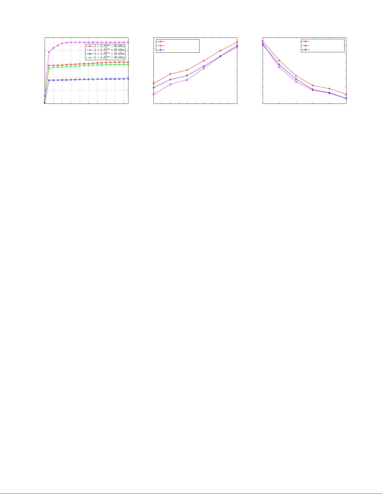
W eighted Sum-Rate Maximization for RIS-U A V -assisted Space-Air -Ground Inte grated Network with RSMA Jian He ∗ , Cong Zhou ∗ , Shuo Shi ∗ ∗ School of Electronics and Information Engineering, Harbin Institute of T echnology , Harbin, China Abstract —In this paper , a rate-splitting multiple ac- cess (RSMA) based joint optimization framework f or the space–air–ground integrated network (SA GIN) is proposed, where the satellite and base stations employ unif orm planar array (UP A) antennas for signal transmission, and unmanned aerial vehicles (U A Vs) relay the satellite signals. Earth stations (ESs) and user equipments (UEs) recei ve signals from satellite and base stations (BSs), respecti vely , r esulting in mutual interference. W e first model the channels and signals in this scenario and analyse the interference at BSs and UEs. Then, W e formulate a joint op- timization problem aimed at maximizing the weighted sum-rate, in volving beamforming, RIS-U A V deployment and phase shifts, and rate splitting. However , this problem is highly non-con vex. T o tackle this challenge, we apply a block coordinate descent (BCD) approach to decompose the problem and employ the weighted minimum mean square error (WMMSE) method to transform the non-con vex objective function. F or the rate-splitting sub- problem, a greedy algorithm is proposed and a successi ve con vex approximation (SCA) algorithm is used for beamforming . Besides, the alter nating direction method of multipliers (ADMM) algorithm is employed for the RIS phase-shift problem with unit- modulus constraints, and an exhaustive search method is adopted for the complex U A V positioning and orientation. Simulation results validate that the proposed algorithm achieves superior performance in terms of user weighted sum-rate. I . I N T RO D U C T I O N W ith the rapid growth of global communication services, the demand for ubiquitous, high-data-rate, and lo w-latency com- munications has been continuously increasing [1]. Ho wever , traditional terrestrial communication networks are constrained by geographical en vironments, infrastructure limitations, and natural disasters, making it dif ficult to achiev e seamless cov- erage in complex or remote areas [2] [3]. T o address these challenges, the space–air–ground integrated network (SA GIN) [4] has been recognized as one of the ke y architectures for 6G. By integrating satellite, aerial, and terrestrial netw orks, SA GIN enables global, three-dimensional, and intelligent communica- tion connectivity [5]. In this architecture, terrestrial networks handle high-density and high-data-rate demands, space-based networks provide global cov erage, and aerial platforms offer dynamic coverage compensation. Howe ver , the integration of multi-layer heterogeneous systems in SAGIN also introduces significant challenges in resource coordination and interfer - ence management. The dynamic mobility of aerial platforms and the comple xity of communication channels further in- crease the difficulty of system design and optimization [6]. Among various enabling technologies, unmanned aerial vehicles (U A Vs) hav e emerged as key relay nodes in SA- GIN due to their flexible deployment and controllable mobil- ity , which enhance coverage and link quality [7]. In recent years, the concept of integrating reconfigurable intelligent surfaces (RIS) with U A Vs, forming a RIS-U A V architecture, has attracted gro wing attention [8]. By adjusting the phase shifts of its reflecting elements, the RIS can intelligently reconfigure the propagation environment [9], while the U A V’ s three-dimensional mobility allows dynamic adjustment of the reflection position, thereby establishing virtual line-of-sight (LoS) links in complex terrains. Meanwhile, rate-splitting multiple access (RSMA), as a nov el multiple access scheme, can effecti vely manage multi-user interference and impro ve spectral efficienc y through message splitting and partial in- terference decoding [10]. Incorporating RSMA into SAGIN can significantly enhance system performance. Ho wever , it also introduces strong coupling among beamforming design, U A V deployment, and RIS phase-shift optimization, leading to a highly non-con ve x problem. This paper in vestigates a joint optimization framework for satellite and terrestrial beamforming, RIS-U A V three-dimensional deployment, and RSMA rate allocation to enhance the overall performance of the communication system. I I . S Y S T E M M O D E L The system model is illustrated in the Fig.1. W ithin the cov erage area of a low earth orbit (LEO) satellite, there are numerous terrestrial cells, each comprising a BS, an earth station (ES), an RIS-U A V and multiple UEs. The LEO satellite serves the ESs, each of which is assisted by a dedicated RIS-U A V to enhance the signal quality . Meanwhile, the BS equipped with a UP A, using the same frequency f as the LEO satellite, provides downlink services to the UEs. Moreover , the LEO satellite is also equipped with the UP A. A. Channel Model Satellite downlink model: In the downlink, the LEO satel- lite, located at an altitude of H S and consisting of N S = N S x × N S y antennas, serves K ESs within the same time slot. Hence, with k ∈ K ≜ { 1 , 2 , ..., K } , the channel between the LEO satellite and k -th ES can be expressed as h k = s N S G ( φ k, 1 ) β k ξ k · a S ( θ ES S ,k , ϕ ES S ,k ) , ∀ k ∈ K , (1) Cell 1 Cell K ,1 k  ,2 k  BS 1 ES 1 UE 1,1 UE 1, L UE K ,1 UE K , L BS K ES K Central axis Beam Other Cel ls ... LEO S a te llite Desir e d Link Interferi ng Link Coverag e Area Fig. 1: System model of considered SA GIN. where β k and ξ k denote the free-space path loss and rain attenuation, respectiv ely . The β k can be obtained using the expression β k = (4 π d ES k /λ ) 2 with d ES k and λ denoting the distance from the satellite to the k -th ES and the wa velength, respectiv ely . The dB form of ξ k follows a log-normal distri- bution ln( ξ dB k ) ∼ N ( µ, σ 2 ) [11]. In addition, G ( φ k, 1 ) in (1) denotes the receiv e antenna gain at the ES as [12] G dBi ( φ ) =      G dBi max − 0 . 0025( D · φ λ ) 2 , φ ∈ [0 , φ m ) 32 − 25 log ( φ r ) , φ ∈ [ φ m , φ r ] max(32 − 25 log φ, − 10) , φ ∈ ( φ r , π ] , (2) where G max = η ( πD /λ ) 2 denotes the maximum antenna gain. In addition, φ m = 20( λ/D ) p G dBi max − 32 − 25 log ( φ r ) and φ r = 15 . 85( D /λ ) − 0 . 6 . Furthermore, a S ( θ ES S ,k , ϕ ES S ,k ) ∈ C N S × 1 in (1), with θ ES S ,k ∈ [0 , π / 2] and ϕ ES S ,k ∈ [ − π , π ] denoting the ele vation and azimuth angles of the ES, represents the steering vector a S ( θ ES S ,k , ϕ ES S ,k ) = 1 √ N S a S ,x ( θ ES S ,k , ϕ ES S ,k ) ⊗ a S ,y ( θ ES S ,k , ϕ ES S ,k ) , (3) where a S ,x ( θ ES S ,k , ϕ ES S ,k ) ∈ C N Sx × 1 and a S ,y ( θ ES S ,k , ϕ ES S ,k ) ∈ C N Sy × 1 are channel response vectors in two directions, re- spectiv ely . Moreover , with N x ≜ { 1 , 2 , ..., N S x } and N y ≜ { 1 , 2 , ..., N S y } , the elements of them can be expressed as: [ a S ,x ( θ ES S ,k , ϕ ES S ,k )] n x = e ȷ 2 π λ d 0 ( n x − 1) sin θ ES S ,k cos ϕ ES S ,k , ∀ n x ∈ N x , (4) [ a S ,y ( θ ES S ,k , ϕ ES S ,k )] n y = e ȷ 2 π λ d 0 ( n x − 1) sin θ ES S ,k sin ϕ ES S ,k , ∀ n y ∈ N y , (5) where d 0 represents the inter-antenna spacing. Furthermore, the channel from the satellite to the k -th RIS-U A V with height H R can be represented by G k ∈ C N R × N S with N R = N R x × N R y denoting the number of elements of the RIS. In addition, denoting the channel from the k -th RIS-U A V to the ES and the RIS phase shift matrix by g k ∈ C N R × 1 and Ψ k ∈ C N R × N R , the equiv alent channel ˜ h k ∈ C N S × 1 can be expressed as ˜ h H k = h H k + g H k Ψ k G k , ∀ k ∈ K , (6) where Ψ k = diag ( e ȷψ k, 1 , e ȷψ k, 2 , ...e ȷψ k,N R ) . Besides, we as- sume that the k -th U A V is aligned with the central axis of the parabolic antenna at the k -th ES, i.e., φ k, 2 = 0 . BS downlink model: The BS equipped with N B = N B x × N B y antennas UP A in the k -th cell pro vides services to L UEs with single antenna in the same time slot. Particularly , we denote the height of UP A by H B and assume that all UEs serviced by the k -th BS are at the same height as the k -th ES. Moreov er, with L ≜ { 1 , 2 , ..., L } , the ele vation and azimuth angles of the l -th UE relati ve to the UP A of BS are denoted by θ U k,l and ϕ U k,l , respecti vely . Hence, the channel from the BS to the l -th UE v k,l ∈ C N B × 1 can be expressed as v k,l = λ √ N B 4 π d U k,l · b ( θ U k,l , ϕ U k,l ) , ∀ k ∈ K , l ∈ L , (7) where d U k,l represents the distance from the BS to l -th UE. There are two ways to ignore the energy leakage from the BS to RIS-U A V : we can deploy the U A V at a suf ficiently high altitude, or orient the RIS reflection surface to ward the ES while placing the BS on the backside of the RIS. Interfering link model: W e use f k,l , q k,l and u k to repre- sent the channel gain from the satellite to UE, from RIS-U A V to UE and from the BS to the ES, and it is obvious that they are similar to h k , g k and v k,l , respectiv ely . Assuming that the array plane at the satellite lies in the x- y plane which is parallel to the ground plane, the coordinate of the k -th ES is giv en by Q E , S 0 k = ( x E k , y E k , z E k ) T in this 3D Cartesian coordinate system defined by S 0 . Analogously , the coordinate of l -th UE of k -th cell in S B k is giv en by Q U , S B k k,l = ( x U k,l , y U k,l , z U k,l ) T . Similarly , the coordinate system S R k is defined such that the k -th RIS lies in the x-y plane, with its facing direction aligned with the z- axis. Furthermore, gi ving the rotation matrix and translation vector from S 0 to S R k by R R k ∈ R R ≜ { R R k } K k =1 and t R k ∈ t R ≜ { t R k } K k =1 , respecti vely , the ele vation and azimuth angle can be obtained to calculate g k , G k , f k,l , q k,l and u k . B. Signal Model Both the satellite and the BSs employ RSMA for signal transmission. Denoting common and priv ate steam by s S c and s S k , the signal transmitted by the satellite can be expressed as x S = w S c s S c + K X k =1 w S k s S k , ∀ k ∈ K ≜ 1 , 2 , ..., K , (8) where the w S c and w S k ∈ C N S × 1 represent the beamforming vector . Similarly , the signal of the k -th BS can be gi ven by x B k = w B k, c s B k, c + L X l =1 w B k,l s B k,l , ∀ k ∈ K , (9) where the w B k, c and w B k,l ∈ C N B × 1 denote the beamforming vector at the k -th BS. With ˜ f H k,l denoting the channel from satellite to l -th UE as (10), the received signal at the ES and UE can be e xpressed as (11) and (12), where n E k and n U k,l denotes the Additiv e White Gaussian Noise (A WGN). ˜ f H k,l = f H k,l + q H k,l Ψ k G k . (10) W ith E {| s S k | 2 } = 1 and E {| s B k,l | 2 } = 1 , the associated signal- to-interference-plus-noise ratio (SINR) can be expressed as γ E,c k = | ˜ h H k w S c | 2 K P j =1 | ˜ h H k w S j | 2 + | u H k w B k,c | 2 + L P j =1 | u H k w B k,j | 2 + P E k , (13) y E k = ˜ h H k x S + u H k x B k + n E k = ˜ h H k w S c s S c | {z } common signal + ˜ h H k w S k s S k | {z } priv ate signal + ˜ h H k K X j  = k w S j s S j | {z } multi-ES interference + u H k w B k, c s B k, c + u H k L X j =1 w B k,j s B k,j | {z } interference from k -th BS + n E k . (11) y U k,l = v H k,l x B k + ˜ f H k,l x S + n U k,l = v H k,l w B k, c s B k, c | {z } common signal + v H k,l w B k,l s B k,l | {z } priv ate signal + v H k,l L X j  = l w B k,j s B k,j | {z } multi-UE interference + ˜ f H k,l w S c s S c + ˜ f H k,l K X j =1 w S j s S j | {z } interference from satellite + n U k,l . (12) γ E,p k = | ˜ h H k w S k | 2 K P j  = k | ˜ h H k w S j | 2 + | u H k w B k,c | 2 + L P j =1 | u H k w B k,j | 2 + P E k , (14) γ U,c k,l = | v H k,l w B k, c | 2 L P j =1 | v H k,l w B k,j | 2 + | ˜ f H k,l w S c | 2 + K P j =1 | ˜ f H k,l w S j | 2 + P U k,l , (15) γ U,p k,l = | v H k,l w B k,l | 2 L P j  = l | v H k,l w B k,j | 2 + | ˜ f H k,l w S c | 2 + K P j =1 | ˜ f H k,l w S j | 2 + P U k,l , (16) where P E k and P U k,l denote the noise power . Moreover , the rates of common streams are represented by r E k and r U k,l , and the total rates of the ES and UE can be expressed as R E k = r E k + log 2 (1 + γ E,p k ) , (17) R U k,l = r U k,l + log 2 (1 + γ U,p k,l ) . (18) C. Pr oblem F ormulation W e assign the weight as P K k =1 P L l =0 α k,l = 1 and the problem can be formulated as ( P1 ) max Ξ ˜ f ( Ξ ) = K X k =1 α k, 0 R E k + K X k =1 L X l =1 α k,l R U k,l (P1.a) s.t. r E k , r U k,l ≥ 0 , ∀ k ∈ K , ∀ l ∈ L , (P1.b) K X k =1 r E k ≤ min k log 2 (1 + γ E,c k ) , (P1.c) L X l =1 r U k,l ≤ min l log 2 (1 + γ U,c k,l ) , ∀ k ∈ K , (P1.d) ∥ w S c ∥ 2 + K X k =1 ∥ w S k ∥ 2 ≤ P S max , (P1.e) ∥ w B k, c ∥ 2 + L X l =1 ∥ w B k,l ∥ 2 ≤ P B max , ∀ k ∈ K , (P1.f) 0 ≤ ψ k,j < 2 π , ∀ k ∈ K , j = 1 , 2 , ..., N R , (P1.g) ( R R k ) T R R k = I , det( R R k ) = 1 , ∀ k ∈ K (P1.h) Q R , S 0 k ∈ X k , ∀ k ∈ K , (P1.i) [ Q S , S R k ] 3 , [ Q E , S R k k ] 3 > 0 , ∀ k ∈ K , (P1.j) R E k ≥ R E min , R U k,l ≥ R U min , ∀ k ∈ K , l ∈ L . (P1.k) where Ξ ≜ { w S , w B , Ψ , r E , r U , R R , t R } with w S ≜ ( w S c , w S 1 , ... w S K ) , w B ≜ ( w B 1 , c , w B 1 , 1 , ... w B K,L ) , Ψ ≜ ( Ψ 1 , Ψ 2 , ..., Ψ K ) , r E ≜ ( r E 1 , r E 2 , ..., r E K ) and r U ≜ ( r U 1 , 1 r U 1 , 2 , ..., r U K,L ) . Constrains (P1.b)(P1.c) and (P1.d) ensure that the rates of common streams are finite and non-negati ve. Additionally , (P1.e) and (P1.f) are the maximum transmit power constraints at the satellite and BSs, respecti vely . (P1.g) corresponds to the phase constraint of the RIS. Moreover , constrain (P1.h) ensures that R R k is a valid rotation matrix which preserves lengths and angles. (P1.i) is the position constrain. Besides, (P1.j) indicates that both the satellite and k - th ES are in the forw ard half-space. (P1.k) is the QoS constrain of the ESs and UEs. I I I . P RO P O S E D A L G O R I T H M T o resolv e this complex problem, we employ the WMMSE approach to transform it into an equi valent form, and at the same time employ block coordinate descent (BCD) algorithm to split (P1) into se veral more manageable sub-problems, which can be solved by con verting its objecti ve function and constraints into con vex forms. A. Optimizing { r E , r U } Given { w S , w B , Ψ , R R , t R } The sub-problem (P1.1) can be formulated as follows with { w S , w B , Ψ , R R , t R } within the feasible region. ( P1.1 ) max r E , r U K X k =1 α k, 0 r E k + K X k =1 L X l =1 α k,l r U k,l (P1.1.a) s.t. ( P1.b ) , ( P1.c ) , ( P1.d ) , ( P1.k ) . (P1.1.b) T o facilitate analysis, the constraints (P1.b) and (P1.k) are organized as r E k ≥ max { 0 , R E min − log 2 (1 + γ E,p k ) } , (19) r U k,l ≥ max { 0 , R U min − log 2 (1 + γ U,p k,l ) } . (20) Hence, the problem (P1.1) with constrains (P1.c), (P1.d), (19) and (20) can be solved by a greedy algorithm as follo ws. First, the rate is allocated to each ES or UE to satisfy all the lower -bound constraints. Then, under the condition that the upper-bound constraints are met, the remaining rate is fully allocated to the ES or UE with the highest weight. B. Equivalent F orm of the Pr oblem (P1) When optimizing the remaining variables, we define Υ ≜ { w S , w B , Ψ , R R , t R } and employ the WMMSE algorithm to transform problem (P1) into the following form [13]. ( P2 ) min Υ , µ , ω K X k =1 L X j =0 α k,j ( ω k,j e k,j − log ( ω k,j )) (P2.a) s.t. ( P1.e ) − ( P1.k ) , (P2.b) where e k,j = E [ | µ k,j y k,j − s k,j | 2 ] , and can be expanded as e k, 0 = | µ k, 0 | 2 ( K X j =1 | ˜ h H k w S j | 2 + | u H k w B k, c | 2 + L X j =1 | u H k w B k,j | 2 + P E k ) − 2 Re { µ k, 0 ˜ h H k w S k } + 1 , (21) e k,l = | µ k,l | 2 ( L X j =1 | v H k,l w B k,j | 2 + | ˜ f H k,l w S c | 2 + K X j =1 | ˜ f H k,l w S j | 2 + P U k,l ) − 2 Re { µ k,l v H k,l w B k,l } + 1 , ∀ l ∈ L . (22) In each optimization iteration, we update µ and ω : µ ∗ k, 0 = ˜ h H k w S k K P j =1 | ˜ h H k w S j | 2 + | u H k w B k, c | 2 + L P j =1 | u H k w B k,j | 2 + P E k , (23) µ ∗ k,l = v H k,l w B k,l L P j =1 | v H k,l w B k,j | 2 + | ˜ f H k,l w S c | 2 + K P j =1 | ˜ f H k,l w S j | 2 + P U k,l , (24) e ∗ k,j = e k,j ( Υ , µ ∗ k,j ) , ω ∗ k,j = 1 e ∗ k,j . (25) Then, we can optimize Υ by solving the following problem. ( P3 ) min Υ K X k =1 L X j =0 α k,j ω ∗ k,j e ∗ k,j (P3.a) s.t. ( P2.b ) . (P3.b) C. Optimizing { w S , w B } Given { r E , r U , Ψ , R R , t R } The sub-problem (P3.1) can be formulated as follows. ( P3.1 ) min w S , w B f ( w S , w B ) (P3.1.a) s.t. ( P1.c ) − ( P1.f ) , ( P1.k ) , (P3.1.b) where f ( w S , w B ) can be expanded as (26). In addition, the constraint (P1.k) can be reformulated as Γ E k ( K P j  = k | ˜ h H k w S j | 2 + | u H k w B k,c | 2 + L P j =1 | u H k w B k,j | 2 + P E k ) ≤ f S , (27) Γ U k,l ( L P j  = l | v H k w B k,j | 2 + | ˜ f H k,l w S c | 2 + K P j =1 | ˜ f H k,l w S j | 2 + P U k,l ) ≤ f B , (28) where Γ E k = 2 ( R E min − r E k ) − 1 and Γ U k,l = 2 ( R U min − r U k,l ) − 1 . Moreov er, the abov e f S and f B are the first-order T aylor expansions of | ˜ h H k w S k | 2 and | v H k,l w B k,l | 2 at point w S ∗ k and w B ∗ k,l , respectiv ely . f S = | ˜ h H k w S ∗ k | 2 + 2 Re { ˜ h H k w S ∗ k ˜ h H k ( w S k − w S ∗ k ) } , (29) f B = | v H k,l w B ∗ k,l | 2 + 2 Re { v H k,l w B ∗ k,l v H k,l ( w B k,l − w B ∗ k,l ) } . (30) Additionally , defining Γ E,c ≜ 2 P K k =1 r E k − 1 and Γ U,c k ≜ 2 P L l =1 r U k,l − 1 , the constraints (P1.c)(P1.d) can be written as Γ E,c ( K P j =1 | ˜ h H k w S j | 2 + | u H k w B k,c | 2 + L P j =1 | u H k w B k,j | 2 + P E k ) ≤ f S,c , (31) Γ U,c k ( L P j =1 | v H k,l w B k,j | 2 + | ˜ f H k,l w S c | 2 + K P j =1 | ˜ f H k,l w S j | 2 + P U k,l ) ≤ f B,c , (32) where f S,c and f B,c are the first-order T aylor expansions of | ˜ h H k w S c | 2 and | v H k,l w B k, c | 2 that are similar to above (29) and (30). At this point, the objective function (26) can be solved by the CVX toolbox. D. Optimizing Ψ Given { w S , w B , r E , r U , R R , t R } The sub-problem can be formulated as ( P3.2 ) min Ψ g ( Ψ ) (P3.2.a) s.t. ( P1.c )( P1.d )( P1.g )( P1.k ) , (P3.2.b) where g ( Ψ ) is e xpanded as (33) and can be rearranged as g ( ζ ) = m + K X k =1 K +( K +1) L X j =1 | ζ T k c k,j | 2 + K X k =1 ( K +1)( L +1) X j =1 Re { ζ T k d k,j } , (34) where ζ ≜ [ ζ 1 , ζ 2 , ..., ζ K ] and m represents the com- plex constant unrelated to ζ . Furthermore, the constraints (P1.c)(P1.d)(P1.k) can be reformulated as Γ E,c ( K X j =1 | h H k w S j + ζ T k diag( g H k ) G k w S j | 2 + | u H k w B k,c | 2 (35) + L X j =1 | u H k w B k,j | 2 + P E k ) ≤ g S,c , Γ U,c k ( L X j =1 | v H k,l w B k,j | 2 + | f H k,l w S c + ζ T k diag( q H k,l ) G k w S c | 2 (36) + K X j =1 | f H k,l w S j + ζ T k diag( q H k,l ) G k w S j | 2 + P U k,l ) ≤ | v H k,l w B k, c | 2 , Γ E k ( K X j  = k | h H k w S j + ζ T k diag( g H k ) G k w S j | 2 + | u H k w B k,c | 2 (37) + L X j =1 | u H k w B k,j | 2 + P E k ) ≤ g S , Γ U k,l ( L X j  = l | v H k,l w B k,j | 2 + | f H k,l w S c + ζ T k diag( q H k,l ) G k w S c | 2 (38) + K X j =1 | f H k,l w S j + ζ T k diag( q H k,l ) G k w S j | 2 + P U k,l ) ≤ | v H k,l w B k,l | 2 , where g S,c and g S are the first-order T aylor expansions of | ˜ h H k w S c | 2 and | ˜ h H k w S k | 2 at ζ ∗ . Additionally , (P1.g) can be rewritten as | [ ζ k ] i | = 1 , ∀ k ∈ K , i = 1 , 2 , ..., N R . (39) Using alternating direction method of multipliers (ADMM) to handle (39) with a positi ve penalty parameter ρ [14], (P3.2) can be reformulated as ( P3.3 ) min ζ , Z , Y g ( ζ ) + ρ 2 ∥ ζ − Z + Y ∥ 2 − ρ 2 ∥ Y ∥ 2 (P3.3.a) s.t. ( 35 )( 36 )( 37 )( 38 ) , (P3.3.b) ζ = Z , (P3.3.c) [ | Z | ] k,i = 1 , ∀ k ∈ K , i = 1 , 2 , ..., N R . (P3.3.d) f ( w S , w B ) = K X k =1 α k, 0 ω k, 0 ( | µ k, 0 | 2 ( K X j =1 | ˜ h H k w S j | 2 + | u H k w B k, c | 2 + L X j =1 | u H k w B k,j | 2 ) − 2 Re { µ k, 0 ˜ h H k w S k } )+ K X k =1 L X l =1 α k,l ω k,l ( | µ k,l | 2 ( L X j =1 | v H k,l w B k,j | 2 + | ˜ f H k,l w S c | 2 + K X j =1 | ˜ f H k,l w S j | 2 ) − 2 Re { µ k,l v H k,l w B k,l } ) (26) g ( Ψ ) = K X k =1 α k, 0 ω k, 0 ( | µ k, 0 | 2 K X j =1 | ( h H k + g H k Ψ k G k ) w S j | 2 − 2 Re { µ k, 0 ( h H k + g H k Ψ k G k ) w S k } )+ K X k =1 L X l =1 α k,l ω k,l | µ k,l | 2 ( | ( f H k,l + q H k,l Ψ k G k ) w S c | 2 + K X j =1 | ( f H k,l + q H k,l Ψ k G k ) w S j | 2 ) (33) In each iteration of ADMM, the update methods for each variable are as follows: ζ ∗ = arg min ζ g ( ζ ) + ρ 2 ∥ ζ − Z + Y ∥ 2 , (40) Z ∗ = arg min [ | Z | ] k,i =1 ∥ ζ ∗ − Z + Y ∥ 2 , (41) Y ∗ = Y + ζ ∗ − Z ∗ . (42) When updating Z , there is an analytical solution as [ Z ] k,i = [ ζ ∗ ] k,i + [ Y ] k,i | [ ζ ∗ ] k,i + [ Y ] k,i | . (43) The iteration terminates when both the primal and dual residuals, expressed as ∥ ζ − Z ∥ and ρ ∥ Z − Z ∗ ∥ , satisfy the required accuracy . E. Optimizing R R , t R Given { w S , w B , Ψ , r E , r U } Giv en any feasible { w S , w B , r E , r U , Ψ } and omitting vari- ables unrelated to R R and t R , the sub-problem can be formu- lated as ( P3.4 ) min R R , t R h ( R R , t R ) (P3.4.a) s.t. ( P1.c )( P1.d ) , ( P1.h ) − ( P1.k ) , (P3.4.b) where the objective function h ( R R , t R ) takes the same form as g ( Ψ ) . It is difficult to design a low-complexity algorithm to optimize R R and t R . Howe ver , when the U A V’ s attitude and position accuracy are limited or not strictly required, it is feasible to design an exhausti ve search algorithm. First, we reduce the dimensionality of the optimization variables. According to (P1.h), we can process R R k using the Euler angle decomposition as R R k = R R k,x ( β k,x ) R R k,y ( β k,y ) R R k,z ( β k,z ) , (44) where β k,x , β k,y and β k,z represent the rotation angles around the x , y and z -axes, respectively . Thus, we only need to trav erse the three rotation angles to optimizing R R k . Then, according to (P1.i), we represent the central axis of the k -th parabolic antenna as a straight line in S 0 . Therefore, the coordinates of the RIS can be expressed as Q R , S 0 k = t R k = Q E , S 0 k + b k p k , ∀ k ∈ K , (45) where p k denotes the unit direction vector of the k -th central axis, and b k determines the position of the RIS along the central axis. Furthermore, b k should satisfy the constraint as − H min / [ p k ] 3 ≤ b k ≤ − H max / [ p k ] 3 , ∀ k ∈ K . (46) By follo wing this alternating optimization procedure, the optimal solution to Problem (P3.4) can be obtained. F . Comple xity Analysis It is observed that the complexity of the greedy algo- rithm for solving (P1.1) is linear . In addition, (P3.1) is a quadratically constrained quadratic program (QCQP), which can be transformed into a second-order cone programming (SOCP). The computational complexity of solving an SOCP depends on the number of the second-order cone (SOC) constraints k soc , the dimension of the optimization variables m soc , and the dimension of the SOC constraints n soc , and can be expressed as O ( k 1 / 2 soc ( m 3 soc + m 2 soc P k soc i =1 n soc + P k soc i =1 n 2 soc )) [15]. Therefore, The computational complexity of solving (P3.1) can be approximately expressed as O ( K 7 / 2 L 1 / 2 ( N S + LN B ) 3 log(1 /ϵ C )) , with ϵ C denoting the target optimization precision, when N S , N B ≫ K , L . Similarly , since the up- dates of Z and Y ha ve closed-form solutions, the com- putational comple xity of solving (P3.3) mainly depends on the update of ζ , and can be approximately expressed as O ( K 7 / 2 L 1 / 2 N 3 R log(1 /ϵ D )) , when N R ≫ K , L . Moreo ver , when solving (P3.4), the precision of distance and angle affect the complexity , which is given by O ((1 /ϵ E 1 ) 3 · 1 /ϵ E 2 ) . I V . N U M E R I C A L R E S U L T S A. P arameter Setup and Benchmark Schemes Unless specified otherwise, the parameters of the simula- tions are set as follows. The satellite provides services to the ESs in K = 3 cells. Meanwhile, in each cell, the BS serves L = 2 UEs for data transmission. Both the BS and the satellite are equipped with N S = N B = 8 × 8 = 64 antennas and operate at a frequency of f = 28 GHz. In addition, the RIS-U A V is equipped with N R = 8 × 8 = 64 reflecting elements and the inter-antenna spacing of all UP As is set to half of the wa velength, i.e., d 0 = λ/ 2 . The maximum transmit po wers of the BS and the satellite are set to P B max = 30 dBm and P S max = 5 W , respectiv ely . For simplicity , the noise powers at both the ESs and the UEs are set to P E k , P U k,l = − 80 dBm , ∀ k ∈ K , l ∈ L . Moreov er , the parameters related to rain attenuation are set to µ = − 3 . 125 and σ = 1 . 591 . Under various conditions, we compared the proposed al- gorithm with two benchmark schemes. 1) No-rate-splitting 1 3 5 7 9 11 13 15 17 19 Number of iterations 0 0.5 1 1.5 2 2.5 Weighted sum rate(bit/s/Hz) (a) W eighted sum rate versus iteration num- bers. 20 21 22 23 24 25 26 27 28 29 30 Maximum transmit power of the BS(dBm) 1.2 1.4 1.6 1.8 2 2.2 2.4 Weighted sum rate(bit/s/Hz) Proposed scheme No-rate-splitting scheme No-RIS scheme (b) W eighted sum rate versus maximum transmit power of the BS. 2 3 4 5 6 7 Number of UEs in each cell 0.8 1 1.2 1.4 1.6 1.8 2 2.2 2.4 Weighted sum rate(bit/s/Hz) Proposed scheme No-rate-splitting scheme No-RIS scheme (c) W eighted sum rate versus number of UEs in each cell. Fig. 2: Performance ev aluation of the proposed algorithm scheme : This benchmark scheme is based on the proposed algorithm but excludes the rate-splitting step, aiming to ev al- uate the system performance in the absence of the common stream. 2) No-RIS sc heme : This benchmark scheme is designed to ev aluate the system performance without RIS assistance. B. P erformance Analysis Fig.2a illustrates the con ver gence behaviour of the proposed algorithm under v arious conditions. It can be observed that the algorithm con verges within a finite number of iterations under all settings. Moreover , An increase in the number of UEs or a reduction in transmit power lead to a decrease in the weighted sum rate, primarily due to the reduction in the SINR. Specifically , an increase in the number of UEs not only intensifies interference but also implies that the same transmit power must be distributed among more UEs. Fig.2b and Fig.2c illustrate the trends of the weighted sum rate for the three schemes as the BS transmit po wer and the number of UEs vary , respectiv ely . It can be observed that the weighted sum rate of all three schemes increases with higher transmit po wer or fe wer UEs. In addition, the proposed scheme outperforms the other two schemes, demonstrating that rate splitting and RIS-UA V can provide significant performance gains in this system. V . C O N C L U S I O N S In this paper , we proposed an RIS-U A V -assisted approach to enhance the performance of SA GIN with RSMA, and for - mulated a joint optimization problem in volving beamforming, RIS phase shifts, and the U A V’ s position and orientation. Moreov er, we de veloped a two-layer iterati ve algorithm, where the original problem was decomposed into multiple sub- problems in the outer loop. Furthermore, we designed solution methods for each sub-problem. Numerical results validate the con vergence of the proposed algorithm and demonstrate its performance advantages compared with other schemes. R E F E R E N C E S [1] C.-X. W ang, X. Y ou, X. Gao, X. Zhu, Z. Li, C. Zhang, H. W ang, Y . Huang, Y . Chen, H. Haas, J. S. Thompson, E. G. Larsson, M. D. Renzo, W . T ong, P . Zhu, X. Shen, H. V . Poor , and L. Hanzo, “On the road to 6g: V isions, requirements, key technologies, and testbeds, ” IEEE Communications Surveys & T utorials , vol. 25, no. 2, pp. 905–974, 2023. [2] O. Kodheli, E. Lagunas, N. Maturo, S. K. Sharma, B. Shankar , J. F . M. Montoya, J. C. M. Duncan, D. Spano, S. Chatzinotas, S. Kisselef f, J. Querol, L. Lei, T . X. V u, and G. Goussetis, “Satellite communi- cations in the new space era: A survey and future challenges, ” IEEE Communications Surve ys & T utorials , vol. 23, no. 1, pp. 70–109, 2021. [3] C. Zhou, S. Shi, C. W u, and S. W ei, “Energy efficient uav-assisted communication with joint resource allocation and trajectory optimization in noma-based internet of remote things, ” W ireless Networks , v ol. 30, no. 6, pp. 5361–5374, 2024. [4] J. Liu, Y . Shi, Z. M. Fadlullah, and N. Kato, “Space-air -ground integrated network: A survey , ” IEEE Communications Surveys & T utorials , vol. 20, no. 4, pp. 2714–2741, 2018. [5] Y . Xiao, Z. Y e, M. W u, H. Li, M. Xiao, M.-S. Alouini, A. Al-Hourani, and S. Cioni, “Space-air-ground integrated wireless networks for 6g: Basics, key technologies, and future trends, ” IEEE J ournal on Selected Ar eas in Communications , vol. 42, no. 12, pp. 3327–3354, 2024. [6] S. Y u, X. Gong, Q. Shi, X. W ang, and X. Chen, “Ec-sagins: Edge- computing-enhanced space–air–ground-integrated networks for internet of vehicles, ” IEEE Internet of Things J ournal , vol. 9, no. 8, pp. 5742– 5754, 2022. [7] C. Zhou, S. Shi, C. W u, and Z. Xu, “Noma empo wered energy efficient data collection and wireless power transfer in space-air-ground integrated networks, ” China Communications , vol. 20, no. 8, pp. 17–31, 2023. [8] X. Liu, Y . Y u, F . Li, and T . S. Durrani, “Throughput maximization for ris-uav relaying communications, ” IEEE T ransactions on Intelligent T ransportation Systems , vol. 23, no. 10, pp. 19 569–19 574, 2022. [9] Q. W u, S. Zhang, B. Zheng, C. Y ou, and R. Zhang, “Intelligent reflecting surface-aided wireless communications: A tutorial, ” IEEE T ransactions on Communications , v ol. 69, no. 5, pp. 3313–3351, 2021. [10] Y . Mao, O. Dizdar , B. Clerckx, R. Schober, P . Popovski, and H. V . Poor , “Rate-splitting multiple access: Fundamentals, survey , and future research trends, ” IEEE Communications Surve ys & T utorials , v ol. 24, no. 4, pp. 2073–2126, 2022. [11] ITU-R, “Recommendation ITU-R P .618-14: Propagation data and pre- diction methods required for the design of Earth-space telecommuni- cation systems, ” International T elecommunication Union, T ech. Rep. P .618-14, Aug. 2023. [12] ITU-R, “Reference radiation pattern APEREC026V01, Recommenda- tion ITU-R S.465-6, ” International T elecommunication Union, T ech. Rep. S.465-6, 2022. [13] Q. Shi, M. Razaviyayn, Z.-Q. Luo, and C. He, “ An iteratively weighted mmse approach to distributed sum-utility maximization for a mimo interfering broadcast channel, ” IEEE T ransactions on Signal Processing , vol. 59, no. 9, pp. 4331–4340, 2011. [14] J. Liang, P . Stoica, Y . Jing, and J. Li, “Phase retrie val via the alternat- ing direction method of multipliers, ” IEEE Signal Pr ocessing Letters , vol. 25, no. 1, pp. 5–9, 2017. [15] M. Beko, “Efficient beamforming in cognitiv e radio multicast transmis- sion, ” IEEE T ransactions on Wir eless Communications , vol. 11, no. 11, pp. 4108–4117, 2012.