Parametric generalized spectrum for heavy-tailed time series

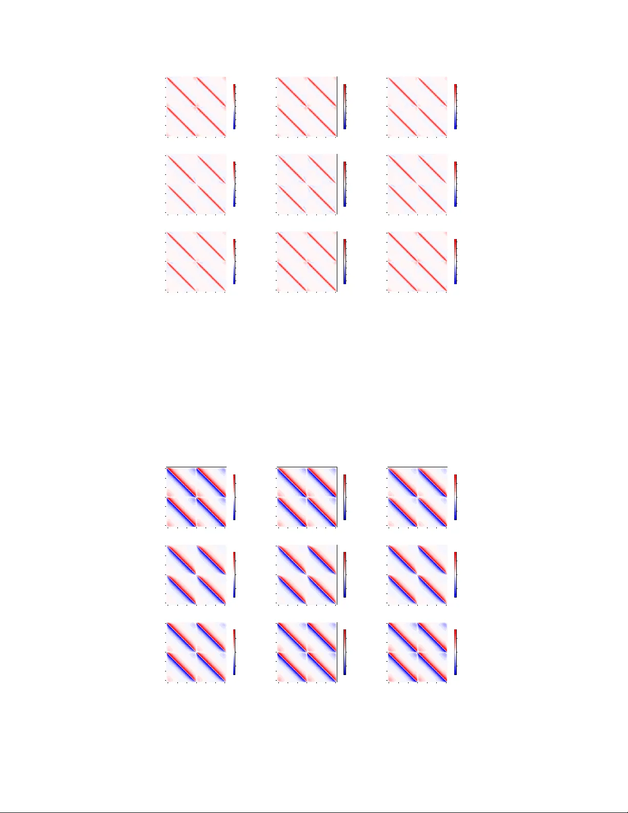
P ARAMETRIC GENERALIZED SPECTR UM FOR HEA VY -T AILED TIME SERIES B Y Y U I C H I G OT O 1 A N D G A S P A R D B E R N A R D 2 1 Faculty of Mathematics , K yushu Univer sity, yuichi.goto@math.kyushu-u.ac.jp 2 Institute of Statistical Science , Academia Sinica, gaspar dbernar d@as.edu.tw Recently , sev eral spectra hav e emerged, designed to encapsulate the dis- tributional characteristics of non-Gaussian stationary processes. This article introduces parametric families of generalized spectra based on the charac- teristic function, alongside inference procedures enabling √ n -consistent es- timation of the unkno wn parameters in a broad class of parametric models. These spectra capture non-linear dependencies without requiring that the un- derlying stochastic processes satisfy any moment assumptions. Crucially , this approach facilitates frequency domain analysis for heavy-tailed time series, including possibly non-causal Cauchy autoregressiv e models and discrete- stable integer-v alued autore gressiv e models. T o the best of our knowledge, the latter models have not been studied theoretically in the literature. By estimating parameters across both causal and non-causal parameter spaces, our method automatically identiﬁes the causal or non-causal structure of Cauchy autoregressiv e models. Furthermore, our estimator does not depend on smoothing parameters since it is based on the integrated periodogram asso- ciated with the generalized spectrum. As applications, we dev elop goodness- of-ﬁt tests, moving average unit-root tests, and tests for non-inv ertibility . W e study the ﬁnite-sample performance of the proposed estimators and tests via Monte Carlo simulations, and apply the methodology to estimation and fore- casting of a measles count dataset. W e e valuate ﬁnite-sample performance using Monte Carlo simulations and illustrate the practical value of the proce- dure with an application to measles case-count estimation and forecasting. 1. Introduction. Spectral methods are widely employed in the analysis of time series data and ha ve found applications in v arious real-world scenarios. In the context of Gaussian processes, the classical spectrum, based on second-order moments, completely captures the distributional characteristics of the time series. Consequently , it stands as one of the most successful techniques for analyzing Gaussian time series data. Howe ver , spectral methods that rely on the classical spectrum, although valid for non-Gaussian processes, suf fer from se veral limitations. First, they fail to capture the distributional characteristics of non-Gaussian processes, as they can only detect linear dependencies and not non-linear ones. Second, these methods require certain moment assumptions to hold, which is in practice often problematic when dealing with dataset known for exhibiting heavy-tailed behaviors such as ﬁnancial data. T o address these issues, se veral new spectra hav e been introduced. One notable advance- ment is the introduction of the g eneralized spectr al density , based on the characteristic func- tion, as proposed by Hong ( 1999 ). Hong ( 1999 ) established the rates of con v ergence of the kernel estimator of the spectrum with respect to the integrated mean squared error while Fokianos and Pitsillou ( 2017 ) and Fokianos and Pitsillou ( 2018 ) dev eloped a test for inde- pendence based on this spectrum. T ests for in v ertibility of v ector autoregressi ve (AR) models with non-Gaussian innov ations based on the generalized spectrum hav e been proposed by Chen et al. ( 2017 ). The spectra based on the joint distrib ution function and copula ha v e been explored by Hong ( 2000 ), later named Laplace spectral density kernel and copula spectral density kernel , respectiv ely , by Dette et al. ( 2015 ). Hong ( 2000 ) and Lee and Rao ( 2012 ) proposed goodness-of-ﬁt tests for the Laplace spectral density , whereas Dette et al. ( 2015 ) 1 2 and Kley et al. ( 2016 ) studied the problem of estimating these spectra. Li ( 2008 ), Li ( 2012 ), Hagemann ( 2013 ), and Li ( 2021 ) studied the Laplace spectrum and quantile spectrum in relation to the copula spectral density kernel. Additionally , V an Hecke et al. ( 2018 ) proposed spectra based on Spearman’ s ρ and Kendall’ s τ . For a comprehensiv e re view on spectral methods, refer to von Sachs ( 2020 ). Ne vertheless, the majority of literature has primarily focused on the development of non- parametric methods, except for Chen et al. ( 2017 ) and V elasco ( 2022 ), leaving the question of explicit closed-form expressions for parametric generalized spectra largely unexplored. Notably , V elasco ( 2022 ) studied the parameter estimation of a non-causal and non-inv ertible parametric inﬁnite-order moving av erage (MA( ∞ )) model with i.i.d. or martingale difference errors based on the generalized spectrum of residuals. An important dif ference with our ap- proach is that V elasco ( 2022 ) does not le verage the closed form of generalized spectra and its study does not encompass moving average (MA) models with unit roots since the recip- rocal of the linear ﬁlter of an inﬁnite-order MA model is used for the calculation of residual from observ ations. Another crucial difference between our results and V elasco ( 2022 ) is that, although the existence of the generalized spectrum itself does not require moment assump- tions, the consistency results for the parametric estimators proposed in V elasco ( 2022 ) still rely on rather stringent ﬁnite-moment conditions. In contrast, our procedure accommodates heavy-tailed inno v ations. Our primary aim in this article is to deri ve explicit forms for the generalized spectra of processes for which the classical deﬁnition of the spectra cannot be used. This includes non- causal and/or non-in vertible processes as well as processes exhibiting inﬁnite variance. Sub- sequently , we tackle the question of estimating the unknown parameters in some models where the closed-form expressions for the parametric generalized spectra allo ws it. Our pa- rameter estimation strategy relies on minimizing a least squares criterion quantifying the discrepancy between the parametric model and the periodogram of the generalized spectrum. It is worth mentioning that our estimation method does not require the use of any smoothing parameter for kernel estimates, a distinct adv antage. T raditionally , the periodogram, while widely used, lacks consistency as an estimator of the spectral density . Consequently , the smoothed periodogram, incorporating some band- width parameter , is typically employed to achiev e consistency . Howe v er , the choice for the bandwidth parameters signiﬁcantly impacts the estimates. T o circumv ent these dif ﬁculties, it is common to consider functionals of the spectra instead. This approach is dev eloped in, for example, Section 7.6 of Brillinger ( 1981 ), Dahlhaus ( 1985 ), and Section 6 of T aniguchi and Kakizaw a ( 2000 ). Notably , the integrated copula spectral density kernel has been recently studied by Goto et al. ( 2022 ). Furthermore, Chiu ( 1988 ) and Preuss et al. ( 2013 ) discussed inference based on some least squares difference for the classical spectral density and the time-v arying spectral density , respectiv ely . Our methodology enables the application of spectral methods to hea vy-tailed time se- ries models, encompassing (continuous) MA and AR models with error processes following stable distrib utions and non-neg ativ e inte ger-v alued MA (INMA) and non-negati v e integer - v alued AR (IN AR) models with error processes follo wing discrete stable distributions. Constructing heavy-tailed non-negati v e integer-v alued time series presents a unique chal- lenge. In practice, count-valued datasets tend to exhibit a few distinctive features. In partic- ular , they are often both ov er-dispersed (i.e., the variance substantially exceeds the mean) and zero-inﬂated (i.e., zeros are overrepresented in the dataset). Nevertheless, there exists an extensi v e literature on non-negativ e integer-v alued time series, including popular mod- els such as the integer-v alued autoregressi v e (INAR) model McKenzie ( 1985 ); Al-Osh and Alzaid ( 1991 ); Latour ( 1997 ) and the integer -valued generalized autoregressi v e conditional heteroscedasticity (INGARCH) model Ferland et al. ( 2006 ). Comprehensiv e revie ws of re- cent de velopments can be found in Da vis et al. ( 2021 ). P ARAMETRIC GENERALIZED SPECTR UM FOR HEA VY -T AILED TIME SERIES 3 INGARCH models require at least that the conditional mean exists, since the model is deﬁned through the autoregressi ve structure of the conditional e xpectation. Gorgi ( 2020 ) e x- plored an INGARCH model based on the beta-neg ativ e binomial distrib ution, which accom- modates heavy tails; howe v er , ﬁnite variance is still assumed to guarantee the ﬁniteness of the asymptotic variance of the estimator . Conv ersely , the IN AR model seems to be able to accommodate hea vy tails by assuming heavy-tailed disturbance processes, but the lack of a zero-median property due to its non-ne gati ve inte ger -valued nature makes the direct applica- tion of the least absolute de viation method problematic. On this note, a major dif ﬁculty in applying LAD to the INAR model stems from the stepwise nature of the conditional median in the integer-v alued setting. In particular , the conditional median of Z t | Z t − 1 = z is not linear in z , which makes centering to enforce a zero-median property more delicate. Note that this issue is speciﬁc to settings that combine integer -v alued models with the absence of a ﬁnite ﬁrst moment. Therefore, to our best knowledge, non-negati v e integer -valued time series models with hea vy-tails ha v e not been de veloped so far . One of the aims of this contrib ution is to propose methods that can be readily applied in such scenarios. As a compelling application of our method, we address the analysis of heavy-tailed integer -v alued data. Figure 1 displays the time series and Hill plots for the measles dataset obtained from Liboschik et al. ( 2017 ). The empirical evidence strongly suggests the pres- ence of heavy tails, with ev en the mean being undeﬁned, as hinted by the Hill estimator plot displayed in Figure 1 . 0 100 200 300 400 500 600 0 50 100 150 Time series of measles cases time index number of cases 50 100 150 200 250 0.0 0.5 1.0 1.5 2.0 2.5 Hill plot for measles cases number of upper order statistics estimated value f or tail index Hill estimator F I G 1 . T ime series plot (left) and Hill plot (right) of the measles dataset. It should also be noted that generalized spectrum is also linked to the notion of distance corr elations , but we do not discuss this fact in detail here. Further details can be found in Davis et al. ( 2018 ); Edelmann et al. ( 2019 ); W an and Davis ( 2022 ), and references therein. It is note worthy that non-causal and non-in vertible autoregressi ve moving average (ARMA) processes possess a causal in vertible representation with the same (classical) spec- tral density as the original process ( Brockwell and Davis , 2009 , p.125–127). In particular, for Gaussian ARMA processes, the causality and in vertibility is required to ensure identiﬁ- ability . For non-Gaussian ARMA processes, for k ≥ 3 , k -th order spectrum is identiﬁable for non-causal and non-in vertible ARMA processes ( V elasco and Lobato , 2018 , Theorem 1). Howe ver , the k -th order spectrum requires at least ﬁnite k -th order moments to exist, which is an assumption that cannot be satisﬁed under heavy tails. Hecq and V elasquez- Gaviria ( 2025 ) identiﬁed non-causal and non-in vertible ARMA models by ﬁrst estimating their causal and in v ertible representation, and then determining the optimal parameters that 4 minimize a chosen criterion across all possible representations. Unlike this approach, our proposed method directly estimates parameters across the causal and non-causal parameter space. Consequently , the resulting estimates automatically identify the causal or non-causal structure of the model. W e ﬁrst deri ve closed-form expressions for the generalized spectrum of processes in sev- eral rele vant parametric heavy-tailed time series models, including the integer -v alued mod- els mentioned earlier . W e then study parameter identiﬁability and propose root- n consistent estimators. Unlike con v entional spectral approaches, our assumptions and proofs extend to generalized spectral densities that may fail to be Hölder continuous—a feature of discrete stable processes—thereby ensuring the v alidity of our methodology in heavy-tailed settings where standard regularity conditions break do wn. The or ganization of the rest of the paper is as follows. Section 2 revie ws the generalized spectrum and its fundamental properties. Section 3 deri ves explicit forms of the generalized spectrum for sev eral models and discusses the identiﬁability of parametric families. Sec- tion 4 presents estimation methods for parametric families of the generalized spectra and in v estigates their statistical properties. Section 5 is dev oted to goodness-of-ﬁt tests for given parametric families. Section 6 dev elops unit-root and non-in vertibility tests for MA models. Section 7 demonstrates the ﬁnite-sample performance of the proposed methods. Section 8 illustrates the utility of our proposed methods via real data analysis. Supplemental material provides proofs of all results and additional ﬁgures and simulation results. 2. Generalized spectrum. W e start by deﬁning the generalized spectrum and stating a fe w of its general properties for a strictly stationary process { Z t } . The generalized spectrum (of order two) is deﬁned, for λ ∈ R and ( u, v ) ∈ R 2 , as f ( λ ; u, v ) : = 1 2 π ∞ X ℓ = −∞ Co v  e iuZ t + ℓ , e − iv Z t  exp ( − iℓλ ) , (1) where i : = √ − 1 , under the summability condition P ∞ ℓ = −∞   Co v  e iuZ t + ℓ , e − iv Z t    < ∞ for all ( u, v ) ∈ R 2 holds. Note that we adopt the con v ention that Co v  e iuZ t + ℓ , e − iv Z t  : = E  e iuZ t + ℓ + iv Z t  − E  e iuZ t + ℓ  E  e iv Z t  . Since ( 1 ) is based on characteristic functions, the construction does not require that { Z t } satisfy any moment assumption. Moreover , unlike the classical spectrum based on the au- tocov ariance function, the generalized spectrum can capture nonlinear serial dependence. It can be readily checked that, from its deﬁnition, the generalized spectrum satisﬁes the follow- ing properties, for any ( u, v ) ∈ R 2 and λ ∈ R , f ( λ ; u, v ) = f ( λ + 2 π ; u, v ) , f ( λ ; u, v ) = f ( − λ ; v , u ) , f ( λ ; u, v ) = f ( − λ ; − u, − v ) , f ( λ ; u, − u ) ∈ R . It is worth mentioning that the pairwise time re versibility of Z t —meaning that the joint distributions of ( Z t , Z t + ℓ ) and ( Z t + ℓ , Z t ) are identical for any ℓ ∈ Z —is equi valent to the spectral symmetry condition f ( λ ; u, v ) = f ( λ ; v , u ) for all ( u, v ) ∈ R 2 and λ ∈ R . Note that if { Z t } is an i.i.d. process, ( 1 ) reduces to f i . i . d . ( λ ; u, v ) : = Cov  e iuZ t , e − iv Z t  / (2 π ) and, thus, the generalized spectrum for any i.i.d. process is a constant function with respect to λ ∈ [ − π , π ] for ﬁxed ( u, v ) ∈ R 2 . P ARAMETRIC GENERALIZED SPECTR UM FOR HEA VY -T AILED TIME SERIES 5 W e now introduce the generalized spectrum of order k , deﬁned for ( λ 1 , . . . , λ k − 1 ) ∈ [0 , 2 π ] k − 1 and ( u 1 , . . . , u k ) ∈ R k as f ( λ 1 , . . . , λ k − 1 ; u 1 , . . . , u k ) : = 1 (2 π ) k − 1 ∞ X ℓ 1 ,...,ℓ k − 1 = −∞ Cum  e iu 1 Z t + ℓ 1 , · · · , e iu k − 1 Z t + ℓ k − 1 , e iu k Z t  exp   − i k − 1 X j =1 ℓ j λ j   , where Cum( Z 1 , · · · , Z k ) is the cumulant of order ℓ deﬁned as Cum( Z 1 , · · · , Z k ) : = X ( ν 1 ,...,ν p ) ( − 1) p − 1 ( p − 1)! E   Y j ∈ ν 1 Z ν 1   . . . E   Y j ∈ ν p Z ν p   . The summation P ( ν 1 ,...,ν p ) extends over all partitions ( ν 1 , . . . , ν p ) of { 1 , 2 , · · · , k } (see Brillinger 1981 , p.19). W e assume that { Z t } satisﬁes the following necessary summabil- ity condition ∞ X ℓ 1 ,...,ℓ k − 1 = −∞    Cum  e iu 1 Z t + ℓ 1 , · · · , e iu k − 1 Z t + ℓ k − 1 , e iu k Z t     < ∞ for all ( u 1 , . . . , u k ) ∈ R k . It is worth noting that Lemma 2.1. of Goto et al. ( 2023 ) implies that the geometrically α -mixing strictly stationary process satisﬁes, for any q ∈ N and any k ∈ N , ∞ X ℓ 1 ,...,ℓ k − 1 = −∞   1 + k − 1 X j =1 | ℓ j | q   × sup ( u 1 ,...,u k ) ∈ R k    Cum  e iu 1 Z t + ℓ 1 , · · · , e iu k − 1 Z t + ℓ k − 1 , e iu k Z t     < ∞ . (2) When considering v arious time series models in Section 3 where stationarity and geomet- ric α -mixing properties have not been established in the literature, we will typically pro vide a similar property , ensuring the existence of generalized spectra. 3. Parametric generalized spectrum. For speciﬁc stochastic processes associated with classical time series models, the explicit form of the generalized spectrum is of particular interest. In this section, we present se veral important e xamples of such parametric spectra. 3.1. Continuous-valued models. W e ﬁrst consider various natural continuous-valued time series models. Throughout this section and the subsequent analysis, we denote by B the backshift oper ator . W e start by deriving a closed form for the generalized spectra in the Cauchy MA(1) and AR(1) models. E X A M P L E 1 . The possibly non-in vertible MA(1) model with Cauchy innov ations and coef ﬁcient a ∈ R 0 : = R \ { 0 } is deﬁned as Z t = (1 − a − 1 B ) ε t , where { ε t } follo ws an i.i.d. Cauchy distrib ution with scale parameter δ > 0 . The generalized spectrum of { Z t } is gi ven by f θ ( λ ; u, v ) = − 1 2 π exp  − δ ( | u | + | v | )( | a − 1 | + 1)  (2 cos λ + 1) + 1 2 π exp  − δ | u + v | ( | a − 1 | + 1)  6 + 1 2 π exp  − δ ( | v a − 1 | + | v + a − 1 u | + | u | )  exp ( − iλ ) + 1 2 π exp  − δ ( | ua − 1 | + | u + a − 1 v | + | v | )  exp ( iλ ) . It is crucial to establish identiﬁability of the model parameters from this parametric fam- ily of generalized spectra. This property is what allows us to perform consistent parameter estimation. L E M M A 1 . In the Cauchy MA(1) model, the vector of parameters θ : = ( a, δ ) ⊤ is identi- ﬁable fr om the g eneralized spectr a. E X A M P L E 2 . The possibly non-causal AR(1) model with Cauchy innov ations and coef- ﬁcient a ∈ R \ {− 1 , 1 } is deﬁned as Z t = aZ t − 1 + ε t , where { ε t } follows an i.i.d. centered Cauchy distribution with scale parameter δ > 0 . The generalized spectrum of this model is gi ven by f θ ( λ, u, v ) = 1 2 π ∞ X ℓ = −∞ C ℓ,a,δ ( u, v ) e − iℓλ , where, for a such that | a | < 1 , C ℓ,a,δ ( u, v ) : = ( exp  − δ 1 −| a |  | ua ℓ + v | + | u | (1 − | a | ℓ )   − exp  − δ ( | u | + | v | ) 1 −| a |  ℓ ≥ 0 C | ℓ | ,a,δ ( v , u ) ℓ < 0 . (3) and for a such that | a | > 1 , C ℓ,a,δ ( u, v ) : = ( exp  − δ | a − 1 | 1 −| a − 1 |  | v a − ℓ + u | + | v | (1 − | a − ℓ | )   − exp  − δ ( | u | + | v | ) | a − 1 | 1 −| a − 1 |  ℓ ≥ 0 C | ℓ | ,a,δ ( v , u ) ℓ < 0 . (4) L E M M A 2 . In the Cauchy AR(1) model, the vector of parameters θ : = ( a, δ ) ⊤ is identi- ﬁable fr om the g eneralized spectr a. Note that, in C ℓ,a,δ ( u, v ) for ℓ > 0 , u and v correspond to the future Z t + ℓ and the current Z t , respectiv ely . The term | ua ℓ + v | in ( 3 ) illustrates that the coefﬁcient a ℓ af fects the v ariable u associated with the future, reﬂecting the causal direction of dependence. In contrast, the term | v a − ℓ + u | in ( 4 ) indicates that the coefﬁcient a − ℓ af fects the v ariable v associated with the current observ ation, reﬂecting the non-causal direction of dependence. L E M M A 3 . The Cauchy AR(1) model enjoys geometrically α -mixing pr operty . Next, we deri ve the generalized spectra for Gaussian MA(1) and AR(1) models. W e con- sider these models due to their extremely classical nature. P ARAMETRIC GENERALIZED SPECTR UM FOR HEA VY -T AILED TIME SERIES 7 E X A M P L E 3. The MA(1) model with Gaussian innovations deﬁned as Z t = (1 − a − 1 B ) ε t , where { ε t } follo ws an i.i.d. centered normal distribution with variance σ 2 . The generalized spectral density is gi ven by f θ ( λ ; u, v ) = 1 2 π exp  − σ 2 2 ( u 2 + v 2 )( a − 2 + 1)  ×  exp  − σ 2 uv ( a − 2 + 1)  − 1 + 2  exp  σ 2 uv a − 1  − 1  cos λ  , where θ : = ( a, σ 2 ) ⊤ such that | a | > 1 and σ 2 > 0 . L E M M A 4 . In the Gaussian MA(1) model, the vector of parameters θ : = ( a, σ 2 ) ⊤ is identiﬁable fr om the g eneralized spectr a. E X A M P L E 4 . The AR(1) model with Gaussian innov ations and coef ﬁcient a such that | a | < 1 is deﬁned as Z t = aZ t − 1 + ε t , where { ε t } follo ws an i.i.d. centered normal distribution with variance σ 2 . The generalized spectrum of this model is gi ven by f θ ( λ, u, v ) = 1 2 π ∞ X ℓ = −∞ C ℓ,a,σ 2 ( u, v ) e − iℓλ , where C ℓ,a,σ 2 ( u, v ) : = e − σ 2 2(1 − a 2 ) ( u 2 + v 2 )  e − σ 2 1 − a 2 uv a | ℓ | − 1  . L E M M A 5 . In the Gaussian AR(1) model, the vector of par ameters θ : = ( a, σ 2 ) ⊤ is iden- tiﬁable fr om the g eneralized spectr a. An important observ ation is that the spectra of Gaussian MA and AR models satisfy the symmetry condition f ( λ, u, v ) = f ( λ, v , u ) , reﬂecting the time-rev ersibility of the process. This implies that the roles of the future variable (associated with u ) and the current variable (associated with v ) can be interchanged without altering the spectrum. 3.2. Discr ete-valued models. Next, we consider heavy-tailed integer -v alued time se- ries models. When constructing a discrete time series model with inﬁnite v ariance, various discrete-v alue distributions with inﬁnite v ariance are av ailable, such as beta-negati v e bino- mial and zeta distrib utions. Howe ver , the characteristic functions of these distributions are often quite complex. One discrete-v alued distribution with inﬁnite variance that possesses a simple characteristic function is the discrete stable distributions introduced by Steutel and v an Harn ( 1979 ). The random v ariable W is said to follow a discrete stable distribution with scale parameter δ > 0 and exponent α ∈ (0 , 1] if the probability generating function (pgf) is giv en by , for x ∈ C such that | x | ≤ 1 , E  x W  = exp {− δ (1 − x ) α } . Thus, the characteristic function of the discrete stable distribution is giv en by E  e isW  = exp {− δ (1 − e is ) α } . If α = 1 , W follows a Poisson distribution. The tail beha vior is characterized by Christoph and Schreiber ( 1998 , Theorem 1) as P( W ≥ n ) = O ( n − α ) , which implies that the fractional moment E ( W m ) is ﬁnite if and only if m < α . 8 The parameters of the discrete-stable innov ations admit straightforward interpretations for count-v alued data. The scale parameter δ directly affects the probability that an innov ation equals zero and is therefore closely linked to the degree of zero inﬂation in the series. By con- trast, the e xponent α gov erns tail hea viness and is thus directly related to the o ver -dispersion of the process. Discrete-stable innov ations therefore provide a ﬂexible mechanism for model- ing the distinctiv e features of count-valued time series. W e consider INMA and INAR models deﬁned through the use of the binomial thinning operator , denoted “ ◦ ” and deﬁned as p ◦ Z t = ( P Z t i =1 Y i,t if Z t > 0 0 if Z t = 0 , for some stochastic process Z t and with { Y i,t } i.i.d. (w .r .t. i and t ) Bernoulli random v ari- ables with parameter p . The binomial thinning operators aims at generalizing the notion of regression coefﬁcient to integer -v alued models, mimicking their effect on the expectation, since E( p ◦ Z t ) = p E( Z t ) (granted that E( Z t ) is ﬁnite). −6 −4 −2 0 2 4 6 −6 −4 −2 0 2 4 6 Real part of spectrum for Example 6 u v −0.15 −0.10 −0.05 0.00 0.05 0.10 0.15 −6 −4 −2 0 2 4 6 −6 −4 −2 0 2 4 6 Imaginary part of spectrum for Example 6 u v −0.15 −0.10 −0.05 0.00 0.05 0.10 0.15 F I G 2 . Heatmaps of the r eal part (left panel) and the imaginary part (right panel) of the spectrum for the causal inte ger -valued AR(1) model in Example 6 , with parameters δ = 2 , p = 0 . 3 , α = 0 . 7 , and λ = 0 . 785 . E X A M P L E 5 . The integer -v alued MA(1) model with discrete stable innov ations is giv en by Z t = p ◦ ε t − 1 + ε t , where “ ◦ ” is the binomial thinning operator deﬁned earlier. { ε t } follows i.i.d. discrete stable distribution with parameters α ∈ (0 , 1] and scale par ameter δ > 0 , and { Y i,k } is independent of { ε t } . Note that the characteristic function of Bernoulli distribution is giv en by E  e isY i,k  = 1 − p + pe is . The generalized spectrum of { Z t } can be expressed as f θ ( λ ; u, v ) : = − 1 2 π exp  − δ  ( p α + 1)  (1 − e iu ) α + (1 − e iv ) α  (2 cos λ + 1) + 1 2 π exp  − δ ( p α + 1)(1 − e i ( u + v ) ) α  + 1 2 π exp  − δ h p α (1 − e iv ) α +  1 − e iv (1 − p + pe iu )  α + (1 − e iu ) α i e − iλ + 1 2 π exp  − δ h p α (1 − e iu ) α +  1 − e iu (1 − p + pe iv )  α + (1 − e iv ) α i e iλ . P ARAMETRIC GENERALIZED SPECTR UM FOR HEA VY -T AILED TIME SERIES 9 The follo wing lemma establishes the crucial identiﬁability property , allo wing to conduct parameter estimation based on the generalized spectrum. L E M M A 6 . In the causal inte ger -valued MA(1) model, the vector of parameters θ θ θ : = ( δ, α, p ) is identiﬁable fr om the generalized spectr a. E X A M P L E 6. The integer-v alued AR(1) with discrete stable inno vations is gi v en by Z t = p ◦ Z t − 1 + ε t . The binomial thinning operator ◦ and the discrete stable distribution are deﬁned as in the pre vious example. The generalized spectrum is f θ ( λ, u, v ) = 1 2 π ∞ X ℓ = −∞ C ℓ,p,δ,α ( u, v ) e − iℓλ , with C ℓ,p,δ,α ( u, v ) : = exp  − δ 1 − p α n (1 − e iu ) α (1 − p αℓ ) +  1 − e iv  1 − p ℓ + p ℓ e iu  α o  − exp  − δ 1 − p α  (1 − e iu ) α + (1 − e iv ) α   for ℓ ≥ 0 C ℓ,p,δ,α ( u, v ) : = C | ℓ | ,p,δ,α ( v , u ) for ℓ < 0 . Here, we used the explicit form of the joint pgf gi v en by: E  u X t  = exp  − δ (1 − u ) α 1 − p α  (5) and E  u X t + ℓ v X t  = exp  − δ (1 − v (1 − p ℓ (1 − u ))) α 1 − p α − δ (1 − u ) α 1 − p αℓ 1 − p α  for ℓ ≥ 0 . (6) Figure 2 sho ws the plot of this spectrum. The proofs of ( 5 ) and ( 6 ) are deferred to Sub- section A.9 . The next lemma guarantees stationarity and the existence of the generalized spectrum. L E M M A 7. If p ∈ (0 , 1) , the inte ger -valued AR(1) model admits a unique strictly station- ary solution, which is er godic. Moreo ver , the inte ger -valued AR(1) model enjoys geometri- cally β -mixing pr operty . R E M A R K 1 . From the proof of Lemma 7 , it is interesting to note that the integer-v alued AR(1) process Z t also follows a discrete stable distribution with exponent α ∈ (0 , 1] and scale parameter δ / (1 − p α ) . Even if such result can be found in the literature, we chose to include here a short and explicit proof for the sake of clarity . Note also at this point that it has been shown–see for instance Corollary 5 in Szücs ( 2024 ) or remark 3 in Basrak et al. ( 2013 )–that the process is in fact geometrically ergodic , which by Theorem 3.7 of Bradley ( 2005 ) directly implies geometrically β -mixing property . The follo wing lemma provides the usual crucial identiﬁcation result. L E M M A 8. In the inte ger -valued AR(1) model, the vector of parameters θ θ θ : = ( δ, α, p ) is identiﬁable fr om the g eneralized spectr a. 10 4. Estimation of unknown parameter . In the previous section, we introduced the para- metric families of generalized spectra. This section is dedicated to the estimation of the un- kno wn parameters of parametric models, based on the generalized spectrum. The parametric family F is deﬁned, for some positiv e integer d and parameter space Θ ⊂ R d , as F : = { f θ ( λ ; u, v ); θ ∈ Θ } . W e assume the following about the parametric family of generalized spectra and about the parameter space. A S S U M P T I O N 1. ( a ) The parameter space Θ is a compact subset of R d . ( b ) The parametric generalized spectrum f θ ( λ ; u, v ) ∈ F is identiﬁable, that is, for given constant L > 0 , f θ ( λ ; u, v ) = f θ ′ ( λ ; u, v ) for all λ ∈ [0 , 2 π ] and ( u, v ) ∈ [ − L, L ] 2 implies θ = θ ′ . ( c ) Let S ⊂ [ − L, L ] 2 be a closed set such that its ε -neighborhood S ε : = { ( u, v ) ∈ [ − L, L ] 2 ; dist(( u, v ) , S ) ≤ ε } satisﬁes Leb( S ε ) = O ( ε ) as ε ↓ 0 , wher e Leb( S ε ) is the Lebesgue measur e of S ε and dist(( u, v ) , S ) : = inf ( x,y ) ∈S ∥ ( u, v ) − ( x, y ) ∥ 2 . Mor eover , ther e exist constants α , β , γ ∈ (0 , 1] , τ ≥ 0 and C ′ > 0 such that, for every ε > 0 , | f θ ( λ ; u, v ) | ≤ C ′ for all ( λ, u, v , θ ) ∈ [0 , 2 π ] × [ − L, L ] 2 × Θ (7) and, for all ( λ, u, v ) , ( λ ′ , u ′ , v ′ ) ∈ [0 , 2 π ] × ([ − L, L ] 2 \ S ε ) and all θ , θ ′ ∈ Θ , | f θ ( λ ; u, v ) − f θ ′ ( λ ′ ; u ′ , v ′ ) | ≤ C ′ ε − τ  | λ − λ ′ | α + ∥ ( u, v ) − ( u ′ , v ′ ) ∥ β + ∥ θ − θ ′ ∥ γ  . (8) W e say that f θ ( λ ; u, v ) is Uniformly Bounded and Partially Hölder continuous except for S , abbr eviated as UBPH( S , τ , α, β , γ ), if the above conditions hold. The assumptions (a) and (b) are e xtremely common. Assumption (c) is necessary to ap- proximate an inte gral by its corresponding Riemann sum at the proper rate. Usually , to obtain the proper rate of con v ergence, Hölder continuity is typically assumed. Howe ver , for the gen- eralized spectra in inte ger-v alued MA and AR models, the deriv ati v es with respect to u or v behav e like u α − 1 , v α − 1 , or ( u + v ) α − 1 for some exponent α ∈ (0 , 1] . This behavior is not compatible with the assumption of uniform Hölder continuity , as the deriv ati ves of the gen- eralized spectra are unbounded around the points u = 0 , v = 0 , and u + v = 0 (mod 2 π ). T o address this issue, we decompose the domain into two parts: (i) a good r e gion , where Hölder continuity holds uniformly , and (ii) a bad r e gion , deﬁned as an ε -neighborhood of the singular set, whose Lebesgue measure is suf ﬁciently small ( S ε in Assumption 1. (c)). This decomposition allo ws us to control the contribution of the singularities while retaining quan- titati ve bounds on the approximation error . In Assumption 1 , the exponents α, β , γ quantify the complexity of the inference problem associated with the global regularity a way from the singularity , while the e xponent τ quantiﬁes the complexity associated with the blow-up rate locally around the singularity . The generalized spectra for the integer -v alued MA(1) and AR(1) models satisfy the assumption (c). The proposed estimation procedure is based on minimizing (with respect to θ ) a suitable criterion. As our criterion, we consider the follo wing L 2 -type di ver gence function: D ( f , f θ ) : = Z 2 π 0 Z L − L Z L − L | f ( λ ; u, v ) − f θ ( λ ; u, v )) | 2 d u d v d λ. P ARAMETRIC GENERALIZED SPECTR UM FOR HEA VY -T AILED TIME SERIES 11 R E M A R K 2 . The choice of integrating over [ − L, L ] 2 with respect to ( u, v ) can seem a little odd at ﬁrst sight b ut is quite natural gi ven that the integer-v alued e xamples presented in Section 3 are periodic. As the focus of this article is integer -v alued models, we then adopt this deﬁnition for the sake of con venience. In all the examples considered in this article, we will chose L = π . R E M A R K 3 . There are instances where spectra can be zero at some λ, u, v , rendering im- possible the use of the contrast-type di ver gences based on f /f θ , including the Whittle-type di ver gence function. F or instance, f ( λ, u, 0) = f ( λ, 0 , v ) = 0 for all ( λ, u, v ) for the inte ger- v alued MA(1) and AR(1) models and the MA(1) and AR(1) models with centered Cauchy errors. In this sense, our method is signiﬁcantly more robust than the Whittle-likelihood meth- ods. These methods rely on the assumption that the spectral density is bounded away from zero, which is often imposed in classical spectral analysis. T o approximate D ( f , f θ ) , we consider D n ( I n , f θ ) : = 8 π L 2 nM 2 n n − 1 X j =1 M n X i 1 ,i 2 =1 | I n ( λ j ; u i 1 , v i 2 ) − f θ ( λ j ; u i 1 , v i 2 )) | 2 , (9) where λ j = 2 π j /n , u i 1 : = − L + 2 Li 1 /M n , v i 2 : = − L + 2 Li 2 /M n , M n ∈ N 0 some param- eter to be speciﬁed in practice and, for any λ ∈ [0 , 2 π ] and ( u, v ) ∈ R 2 , I n ( λ ; u, v ) : = 1 2 π n d n ( λ ; u ) d n ( − λ ; v ) , d n ( λ ; u ) : = n X t =1 e iuZ t e − itλ . The next lemma shows that D n ( I n , f θ ) has a non-negligible bias but ﬁrst, we need to in- troduce some extra notation. Consider sets S and S ε as in Assumption 1 ( c ′ ). W e say that the generalized spectrum of order 2, f ( λ, u, v ) is P artially Hölder continuous except for S ( PH( S , ˜ τ , ˜ α, ˜ β ) ) with exponent ˜ α associated to λ ∈ [0 , 2 π ) and with exponent ˜ β associated to ( u, v ) ∈ [ − L, L ] 2 if there exists C ′ > 0 such that | f ( λ ; u, v ) − f ( λ ′ ; u ′ , v ′ ) | ≤ C ′ ε − ˜ τ  | λ − λ ′ | ˜ α + ∥ ( u, v ) − ( u ′ , v ′ ) ∥ ˜ β  . L E M M A 9 . Consider a family of parametric gener alized spectra satisfying Assumption 1 and a stationary pr ocess Z t satisfying condition ( 2 ) for q = 1 . Assume that the gener alized spectrum of or der two of { Z t } , f ( λ, u, v ) is PH( S , ˜ τ , ˜ α, ˜ β ) . Assume mor eover that, as n → ∞ , M n → ∞ . Then, for any θ ∈ Θ , D n ( I n , f θ ) con ver ges in pr obability to ˜ D ( f , f θ ) as n → ∞ wher e ˜ D ( f , f θ ) : = D ( f , f θ ) + Z 2 π 0 Z L − L Z L − L f ( λ ; u, − u ) f ( − λ ; v , − v )d u d v d λ. As the bias R 2 π 0 R L − L R L − L f ( λ ; u, − u ) f ( − λ ; v , − v )d u d v d λ is independent of θ , D n ( I n , f θ ) can be used for the estimation of the unkno wn parameters θ . W e deﬁne the true value θ 0 and its estimator ˆ θ n by θ 0 : = arg min θ ∈ Θ D ( f , f θ )  = arg min θ ∈ Θ ˜ D ( f , f θ )  and ˆ θ n : = arg min θ ∈ Θ D n ( I n , f θ ) . (10) R E M A R K 4. Our estimator is closely related to Knight and Y u ( 2002 ) who explored pa- rameter estimation based on the joint characteristic function E  e i P p j =0 u j Z t + j  for a strictly stationary and er godic process { Z t } and a ﬁx ed constant p . Their estimator can capture the joint distribution of ( Z t , . . . , Z t + p ) . In contrast, our estimator is based on the bi v ariate char- acteristic functions of ( Z t + ℓ , Z t ) for all ℓ ∈ Z . 12 R E M A R K 5 . Klüppelberg and Mik osch ( 1994 ) in vestigated the self-normalized classical periodogram for MA( ∞ ) process, when the disturbance belongs to the domain of attraction of a stable law . Subsequently , Mikosch et al. ( 1995 ) estimated parameters of ARMA model whose error process belongs to the domain of attraction of a stable law through the use of the self-normalized periodogram. W e assume from no w on that D ( f , f θ ) has a unique minimum at θ 0 ∈ Θ . This condition is fulﬁlled if the model is correctly speciﬁed or , in other words, f ∈ F , but it can also be satisﬁed under certain forms of misspeciﬁcation. Then, the follo wing theorem sho ws that ˆ θ n is a consistent estimator of θ 0 . T H E O R E M 4.1. Consider a family of gener alized spectra satisfying Assumption 1 and a stationary pr ocess Z t satisfying condition ( 2 ) for q = 1 . Assume that the gener alized spectrum of or der two of { Z t } , f ( λ, u, v ) is PH( S , ˜ τ , ˜ α, ˜ β ) . Assume moreo ver that, as n → ∞ , M n → ∞ and that D ( f , f θ ) possesses a unique minimum. The estimator ˆ θ n con ver g es in pr obability to θ 0 as n → ∞ . In the proof of Theorem 4.1 , we sho w that the stochastic equicontinuity of D n ( I n , f θ ) − ˜ D ( f , f θ ) and the pointwise consistenc y of Lemma 9 is suf ﬁcient to yield some uniform la ws of large numbers of the form sup θ ∈ Θ    D n ( I n , f θ ) − ˜ D ( f , f θ )    P → 0 as n → ∞ . As usual, obtaining the asymptotic normality requires some more stringent regularity as- sumptions. W e show that under the assumption that f θ is twice continuously differentiable with respect to θ with deri v ati ves of UBPH, ˆ θ n is asymptotically normal with the usual para- metric con v ergence rates. A S S U M P T I O N 2. ( d ) The parametric spectrum f θ ( λ ; u, v ) is twice differ entiable with r espect to θ . Its deriva- tives ∂ 2 ∂ θ ∂ θ ⊤ f θ ( λ ; u, v ) and ∂ ∂ θ f θ ( λ ; u, v ) ar e UBPH( S , τ , α, β , γ ), wher e the absolute value on the left-hand sides of ( 7 ) and ( 8 ) is r eplaced by the norm ∥ · ∥ . ( e ) The true value θ 0 belongs to the interior of Θ . ( f ) The matrix J deﬁned in ( 11 ) is invertible . It can be easily checked that the generalized spectra for the INMA(1) and INAR(1) models satisfy Assumption 2 ( d ). R E M A R K 6 . The differentiability condition of f θ with respect to θ excludes MA and AR processes with Cauchy errors studied in Section 3 . A possible way to handle non- dif ferentiable parametric models is to replace the absolute value function | x | with a smooth approximation. For e xample, one may consider the sigmoid-based function ϕ ( x ) : = 2 log(1 + e kx ) /k − x − 2 log(2) /k , where k > 0 . Its deriv ati ve ϕ ′ ( x ) = 2 e kx / (1 + e kx ) − 1 provides a smooth approximation of the sign function. T aking k arbitrarily large, we expect the value of D n deﬁned in ( 9 ) to be nearly identical with and without smoothing. In the simulation study , we do not implement such a smoothing modiﬁcation and simply use the original absolute value function. Never - theless, the empirical results appear to support the asymptotic normality of the estimator . W e are no w ready to state the asymptotic normality result for the proposed estimator ˆ θ n . P ARAMETRIC GENERALIZED SPECTR UM FOR HEA VY -T AILED TIME SERIES 13 T H E O R E M 4.2 . Consider a family of parametric generalized spectra satisfying Assump- tions 1 and 2 and a stationary pr ocess Z t satisfying condition ( 2 ) for q = 1 . Assume that the gener alized spectrum of or der four of { Z t } is partially Hölder ( PH as in Theorem 4.1 ) with arbitrary exponents (note that it implies that second or der generalized spectrum f ( λ, u, v ) is also partially Hölder). Assume that f ( λ, u, v ) is PH( ˜ τ , ˜ α, ˜ β ) with e xponents satisfying min { α, ˜ α, β , ˜ β } max { τ , ˜ τ } + 1 > 1 / 2 . Assume ﬁnally that n → ∞ , n − 1 / 2 M n → ∞ and that D ( f , f θ ) admits a unique minimizer . Then, under these assumptions, √ n ( ˆ θ n − θ 0 ) L → N (0 , J − 1 I J − 1 ) as n → ∞ . Her e, J and I ar e deﬁned as follows: J : = − Z 2 π 0 Z L − L Z L − L f ( λ ; u, v ) ∂ 2 ∂ θ ∂ θ ⊤ f θ ( λ ; u, v )    θ = θ 0 d u d v d λ − Z 2 π 0 Z L − L Z L − L ∂ 2 ∂ θ ∂ θ ⊤ f θ ( λ ; u, v )    θ = θ 0 f ( λ ; u, v )d u d v d λ + Z 2 π 0 Z L − L Z L − L ∂ 2 ∂ θ ∂ θ ⊤  f θ ( λ ; u, v ) f θ ( λ ; u, v )     θ = θ 0 d u d v d λ. (11) and I : =( I st ) s,t =1 ,...,d , I st : = L 1 st + L 2 st + L 3 st + L 4 st . Denoting by δ ( x ) the Dirac delta function center ed in x and with the con vention d w = d u d u ′ d v d v ′ d λ d λ ′ , L 1 st , L 2 st , L 3 st , L 4 st ar e deﬁned as follows: L 1 st : =2 π Z (0 , 2 π ) 2 Z [ − L,L ] 4 h δ ( λ − λ ′ ) f ( λ ; u, v ′ ) f ( − λ ; v , u ′ ) + δ (2 π − λ − λ ′ ) f ( λ ; u, u ′ ) f ( − λ ; v , v ′ ) + f ( λ, − λ, λ ′ ; u, v , u ′ , v ′ ) i × ∂ ∂ θ s f θ ( λ ; u, v )    θ = θ 0 ∂ ∂ θ t f θ ( λ ′ ; u ′ , v ′ )    θ = θ 0 d w , L 2 st : =2 π Z (0 , 2 π ) 2 Z [ − L,L ] 4 h δ ( λ − λ ′ ) f ( λ ; u, − u ′ ) f ( − λ ; v , − v ′ ) + δ (2 π − λ − λ ′ ) f ( λ ; u, − v ′ ) f ( − λ ; v , − u ′ ) + f ( λ, − λ, − λ ′ ; u, v , − u ′ , − v ′ ) i × ∂ ∂ θ s f θ ( λ ; u, v )    θ = θ 0 ∂ ∂ θ t f θ ( λ ′ ; u ′ , v ′ )    θ = θ 0 d w , L 3 st : =2 π Z (0 , 2 π ) 2 Z [ − L,L ] 4 h δ ( λ − λ ′ ) f ( λ ; − v , v ′ ) f ( − λ ; − u, u ′ ) + δ (2 π − λ − λ ′ ) f ( λ ; − v , u ′ ) f ( − λ ; − u, v ′ ) + f ( − λ, λ, λ ′ ; − u, − v , u ′ , v ′ ) i × ∂ ∂ θ s f θ ( λ ; u, v )    θ = θ 0 ∂ ∂ θ t f θ ( λ ′ ; u ′ , v ′ )    θ = θ 0 d w , L 4 st : =2 π Z (0 , 2 π ) 2 Z [ − L,L ] 4 h δ ( λ − λ ′ ) f ( λ ; − v , − u ′ ) f ( − λ ; − u, − v ′ ) 14 + δ (2 π − λ − λ ′ ) f ( λ ; − v , − v ′ ) f ( − λ ; − u, − u ′ ) + f ( − λ, λ, − λ ′ ; − u, − v , − u ′ , − v ′ ) i × ∂ ∂ θ s f θ ( λ ; u, v )    θ = θ 0 ∂ ∂ θ t f θ ( λ ′ ; u ′ , v ′ )    θ = θ 0 d w . R E M A R K 7 . In Theorem 4.2 , note that the integration ov er frequencies in L 1 st , L 2 st , L 3 st , L 4 st is taken on the open domain (0 , 2 π ) 2 , which implies that the Dirac delta functions δ ( · ) do not take v alues on the boundary of the domain. R E M A R K 8 . In Theorem 4.2 , the regularity condition min { α, ˜ α, β , ˜ β } max { τ , ˜ τ } + 1 > 1 / 2 has a natural interpretation. If the generalized spectrum is smoother away from the singularity (larger α, ˜ α, β , ˜ β ), then one can tolerate a faster blow-up of the deriv ati ve near the singularity (larger τ , ˜ τ ), and con v ersely . In other words, the condition quantiﬁes a trade-off between global smoothness and local beha vior around the singularity in our inference problem. If Hölder continuity holds globally (i.e., τ = ˜ τ = 0 ), the condition reduces to min { α, ˜ α, β , ˜ β } > 1 / 2 . Furthermore, if the related generalized spectra are Lipschitz continuous (corresponding to α = ˜ α = β = ˜ β = 1 ), this condition is trivially satisﬁed. 5. Goodness-of-ﬁt test. In statistical analysis, it is often of interest to assess whether a ﬁtted model is appropriate. In this section, we consider a goodness-of-ﬁt test. More precisely , for a gi ven parametric family F = { f θ ( λ ; u, v ) : θ ∈ Θ } , we test the composite hypothesis H 1 : f ∈ F versus K 1 : f / ∈ F . W e observed in the pre vious section that the estimator D n ( I n , f θ ) of the distance D ( f , f θ ) suf fers from the bias term Z 2 π 0 Z L − L Z L − L f ( λ ; u, − u ) f ( λ ; − v , v ) d u d v d λ, which is dif ﬁcult to estimate by nonparametric methods. One might consider using the in- tegrated version of I n ( λ j ; u, − u ) I n ( λ j ; − v , v ) as an estimator of the bias term. Howe ver , Lemma 10 sho ws that E [ I n ( λ j ; u, − u ) I n ( λ j ; − v , v )] = f ( λ j ; u, − u ) f ( λ j ; − v , v ) + f ( λ j ; u, v ) f ( λ j ; − v , − u ) + O (1 /n ) , which indicates that I n ( λ j ; u, − u ) I n ( λ j ; − v , v ) contains a non-negligible bias. T o address this problem, we add an adjustment term A n , where A n is non-negati ve and the bias arising D n + A n is estimable. The non-negati ve restriction pre v ents potential power loss under some alternati ves. Thus, we propose the follo wing test statistic. T n = D n ( I n , f ˆ θ n ) + A n ( I n , f ˆ θ n ) − B n ( I n ) , where A n ( I n , f θ ) : = 4 π L 2 nM 2 n n − 1 X j =1 M n X i 1 ,i 2 =1 | I n ( λ j ; u i 1 , − u i 1 ) − f θ ( λ j ; u i 1 , − u i 1 ) + I n ( λ j ; − v i 2 , v i 2 ) − f θ ( λ j ; − v i 2 , v i 2 ) | 2 , P ARAMETRIC GENERALIZED SPECTR UM FOR HEA VY -T AILED TIME SERIES 15 and B n ( I n ) : = 8 π L 2 nM 2 n n − 1 X j =1 M n X i 1 ,i 2 =1  I 2 n ( λ j ; u i 1 , − u i 1 ) + I 2 n ( λ j ; − v i 2 , v i 2 ) 4 + I n ( λ j ; u i 1 , v i 2 ) ¯ I n ( λ j ; u i 1 , v i 2 ) + I n ( λ j ; u i 1 , − u i 1 ) I n ( λ j ; − v i 2 , v i 2 ) 2  . The term B n corresponds to the bias correction term. W e design T n as the estimator of the quantity D ( f , f θ 0 ) + A ( f , f θ 0 ) , where A ( f , f θ ) : = 1 2 Z 2 π 0 Z L − L Z L − L | f ( λ j ; u, − u ) − f θ ( λ j ; u, − u ) + f ( λ j ; − v , v ) − f θ ( λ j ; − v , v ) | 2 d u d v d λ. The adjustment term A n induces the follo wing biases: Z 2 π 0 Z L − L Z L − L f ( λ ; u, v ) f ( λ ; − v , − u ) + 1 2 f 2 ( λ ; u, − u ) + 1 2 f 2 ( λ ; − v , v )d u d v d λ. Among these, the second and third bias terms are directly estimable. On the other hand, the biases Z 2 π 0 Z L − L Z L − L f ( λ ; u, − u ) f ( λ ; − v , v )d u d v d λ and Z 2 π 0 Z L − L Z L − L f ( λ ; u, v ) f ( λ ; − v , − u )d u d v d λ arising from D n ( I n , f ˆ θ n ) and A n ( I n , f ˆ θ n ) , respecti vely , cannot be estimated individually but can be estimated jointly . The hypothesis can no w be rephrased as follo ws: ˜ H 1 : D 0 ( f , f θ 0 ) + A ( f , f θ 0 ) = 0 versus ˜ K 1 : D 0 ( f , f θ 0 ) + A ( f , f θ 0 ) > 0 . From the proof of Theorem 4.2 , we see that D n ( I n , f ˆ θ n ) = D n ( I n , f θ 0 ) + ∂ ∂ θ D n ( I n , f θ )    θ = θ 0 ( ˆ θ n − θ 0 ) + 1 2  ˆ θ n − θ 0  ⊤ ∂ 2 ∂ θ ∂ θ ⊤ D n ( I n , f θ )    θ = θ ∗ n  ˆ θ n − θ 0  = D n ( I n , f θ 0 ) + O p  1 n  . Thus, the plug-in ef fect is ne gligible for √ nD n ( I n , f ˆ θ n ) . Assume that A ( f , f θ ) has a unique minimum at θ 0 ∈ ˚ Θ to ensure ∂ / ( ∂ θ ) A ( f , f θ ) | θ = θ 0 = 0 . Then, by the same argument, the plug-in ef fect is negligible for √ nA n ( I n , f ˆ θ n ) . Therefore, we obtain T n = D n ( I n , f θ 0 ) + A n ( I n , f θ 0 ) − B n ( I n ) + O p  1 n  . 16 Then, the cumulant ar gument gi ves that √ n ( T n − D 0 ( f , f θ 0 ) − A ( f , f θ 0 )) con v erges in dis- tribution to a normal distribution as n → ∞ . Howe ver , the asymptotic v ariance is v ery com- plex and dif ﬁcult to obtain a precise estimate. Therefore, we employ a sub-sampling method; that is, we reject H 1 whene ver p n, 1 ≤ φ , where p n, 1 : = 1 n − b + 1 n − b +1 X t =1 I n √ bT b,t > √ nT n o and T b,t is deﬁned as T n but based on the subsample { Z t , . . . , Z t + b − 1 } . 6. Hypothesis tests for unit-root and in vertibility . In this section, we propose one- sided and two-sided hypotheses tests based on the subsampling method. Applications of the theory de v eloped in this section include testing for the existence of MA unit roots and for the non-in v ertibility for non-causal MA( d 1 + d 2 ) models with Cauchy residuals. Here, we make the assumption that the parameters of the model can be properly identiﬁed by the parametric generalized spectrum. Closed forms of generalized spectrum for Cauchy MA(1) models have been provided in Section 3 , as well as an identiﬁability result. Theorem 4.2 gi ves the asymptotic distribution of the proposed estimator . Ho we ver , for constructing the asymptotically valid tests (and conﬁdence intervals), the estimation of the asymptotic v ariance is required, which turns out to be a non-tri vial problem. Such a problem has been studied in T aniguchi et al. ( 1996 ), where variance estimation in volv ed some k ernel- based consistent estimator of Z π − π Z π − π ϕ ( λ, λ ′ ) f L 2 ( − λ, λ ′ , − λ ′ )d λ d λ ′ , where ϕ ( · , · ) is a continuous function and f L 2 ( · , · , · ) is the classical fourth order spectrum (see Proposition 1 of T aniguchi et al. 1996 ). As mentioned in the Introduction, selecting an appropriate bandwidth parameter for the smoothed periodogram poses a challenge. More- ov er , tests and conﬁdence intervals based on the estimated asymptotic variance often exhibit unsatisfactory ﬁnite-sample performance. T o address this issue, resampling methods have been in v estigated by se v eral authors. Recently , Meyer et al. ( 2020 ) introduced the hybrid pe- riodogram bootstrap for spectral means and ratio statistics based on the classical spectrum under mild conditions, highlighting the failure of the multiplicative periodogram bootstrap to capture terms in volving fourth-order spectra in variance. Kreiss and Paparoditis ( 2023 ) applied this method to Whittle likelihood estimation. Although the assumptions are mild, they still require for the classical spectrum to be non-zero, which is not necessarily satisﬁed by generalized spectra. In particular, we conﬁrmed earlier that the generalized spectral can be zero, making this approach unsuitable for our speciﬁc problem. In contrast, subsampling methods do not require such a condition and are applicable to a broad range of α -mixing processes. See Politis et al. ( 1999 ) for details. Note also that Goto et al. ( 2022 ) constructed conﬁdence bands and hypothesis tests based on the subsampling method for the integrated copula spectral density kernel. In the follo wing section, we introduce subsampling-based h y- pothesis tests. 6.1. T wo-sided hypothesis. W e start by considering the classical two-sided hypothesis testing problem formulated as H 2 : θ 0 i = κ i versus K 2 : θ 0 i  = κ i , where θ 0 = ( θ 01 , . . . , θ 0 d ) ⊤ . Then, the subsampling-based p -value can be deﬁned as p n, 2 : = 1 n − b + 1 n − b +1 X t =1 I n    √ b  ˆ θ ( i ) b,t − κ     >    √ n  ˆ θ ( i ) n − κ     o , P ARAMETRIC GENERALIZED SPECTR UM FOR HEA VY -T AILED TIME SERIES 17 where ˆ θ ( i ) b,t is the subsample estimator based on { Z t , . . . , Z t + b − 1 } . The follo wing result es- tablishes the asymptotic v alidity and consistency of this test. T H E O R E M 6.1 . Assume that the assumptions of Theorem 4.2 hold. Consider the strictly stationary pr ocess { Z t } is α -mixing with vanishing α -mixing coefﬁcient, and that the sub- sampling bloc k length b satisﬁes b/n → 0 as n → ∞ . The test which r ejects H 2 in favor of K 2 whenever p n, 2 ≤ φ has asymptotic size φ and is consistent. W e demonstrate ho w the abov e can be applied to construct the unit-root test. E X A M P L E 7. Consider MA( d 1 + d 2 ) models with Cauchy residuals for an y nonne gati ve integers d 1 and d 2 , that { Z t } satisﬁes Z t = (1 − ξ − 1 1 B ) · · · (1 − ξ − 1 d 1 B )(1 − ξ d 1 +1 B − 1 ) · · · (1 − ξ d 1 + d 2 B − 1 ) ε t , where ε t follo ws i.i.d. centered Cauchy distribution with scale parameter δ > 0 . The param- eter space Θ for ( ξ 1 , . . . , ξ d 1 + d 2 , δ ) is set to be [ L − 1 , L ] d 1 + d 2 +1 . W e moreover assume that Assumptions 1 (b) and 2 (f) hold. T esting for the presence of an MA unit root in the model comes to considering the follo wing null hypotheses and alternati ves. H 2 , ex : ξ i = 1 versus K 2 , ex : ξ i  = 1 . Denote the subsample estimator based on { Z t , . . . , Z t + b − 1 } and the full sample estimator by ˆ ξ ( i ) b,t and ˆ ξ ( i ) n , respecti vely . Our proposed test rejects H 2 , ex whene ver p n, 2 , ex ≤ φ , where p n, 2 , ex : = 1 n − b + 1 n − b +1 X t =1 I n    √ b  ˆ ξ ( i ) b,t − 1     >    √ n  ˆ ξ ( i ) n − 1     o . It is essential to note that in cases where data undergoes differencing before analysis, the risk of ov er -differencing—which leads to the presence of an MA unit root—must be carefully considered. In this regard, V elasco and Lobato ( 2018 ) and V elasco ( 2022 ) assumed the absence of MA unit roots in the conte xt of the estimation of ARMA parameters based on the higher-order classical spectrum and the generalized spectrum, respecti v ely . 6.2. One-sided hypothesis. Next, we consider for i ∈ { 1 , . . . , d } the one-sided hypothesis testing problem formulated by H 3 : θ 0 i ≤ κ i versus K 3 : θ 0 i > κ i . The subsampling based p -value can be deﬁned as p n, 3 : = 1 n − b + 1 n − b +1 X t =1 I n √ b  ˆ θ ( i ) b,t − κ i  > √ n  ˆ θ ( i ) n − κ i o , where ˆ θ b,t : = ( ˆ θ (1) b,t , . . . , ˆ θ ( d ) b,t ) ⊤ is the subsample estimator based on { Z t , . . . , Z t + b − 1 } and ˆ θ n : = ( ˆ θ (1) n , . . . , ˆ θ ( d ) n ) is the full sample estimator . T H E O R E M 6.2 . Assume that the assumptions of Theorem 4.2 hold. Consider the strictly stationary pr ocess { Z t } is α -mixing with vanishing α -mixing coefﬁcient, and the sub- sampling block length b satisﬁes b/n → 0 as n → ∞ . The test whic h rejects H 3 in favor of K 3 whenever p n, 3 ≤ φ has asymptotic level φ and is consistent. 18 Similarly , we can test the hypothesis H 4 : θ 0 i ≥ κ i versus K 4 : θ 0 i < κ i . by the test which rejects H 4 whene ver p n, 4 ≤ φ , where p n, 4 : = 1 n − b + 1 n − b +1 X t =1 I n √ b  κ i − ˆ θ ( i ) b,t  > √ n  κ i − ˆ θ ( i ) n o . W e conclude this section by demonstrating how our procedures can be used to test for non-in v ertibility . In practice, practitioners typically aim to reject the null hypothesis of non- in v ertibility for the observed process. E X A M P L E 8 . Consider MA( d 1 + d 2 ) models with Cauchy residuals in Example 7 . If | ξ 1 | , . . . , | ξ d 1 + d 2 | > 1 , we have that ε t = 1 (1 − ξ − 1 1 B ) · · · (1 − ξ − 1 d 1 B )(1 − ξ d 1 +1 B − 1 ) · · · (1 − ξ d 1 + d 2 B − 1 ) Z t =   ∞ X j =0 ξ − j 1 B j   · · ·   ∞ X j =0 ξ − j d 1 B j     − ∞ X j =0 ξ − j − 1 d 1+1 B j +1   · · ·   − ∞ X j =0 ξ − j − 1 d 1 + d 2 B j +1   Z t and thus the process is in v ertible. Therefore, the test for non-inv ertibility can be formulated as H 3 , ex : | ξ i | ≤ 1 versus K 3 , ex : | ξ i | > 1 . Then we propose the test rejects H 3 , ex whene ver p n, 3 , ex ≤ φ , p n, 3 , ex : = 1 n − b + 1 n − b +1 X t =1 I n √ b     ˆ ξ ( i ) b,t    − 1  > √ n     ˆ ξ ( i ) n    − 1 o . Note that Chen et al. ( 2017 ) considered a test for inv ertibility for vector ARMA model based on the generalized spectrum for residuals but the y do not consider the unit-root case. 7. Simulation studies. In this section, we illustrate the validity of our mathematical results through some simulation studies. W e cov er both estimation and hypothesis testing. One of the main goals is to sho w that our asymptotic results are of practical use, highlighting that a reasonably lar ge sample size is enough for our proposed procedures to perform well. Our simulation setups are designed to illustrate the rob ustness to the presence of heavy-tailed innov ations. 7.1. Estimation. 7.1.1. Real-valued models. W e ﬁrst consider the continuous case with heavy-tailed in- nov ations. More precisely , we consider the MA (1) and AR (1) processes with Cauchy inno- v ations, deﬁned in Section 3 . In the case of the AR (1) model, we consider both the causal and non-causal cases, as the generalized spectra hav e dif ferent closed form expressions in these two cases. As we sho wed in Section 3 that the parameters ( a, δ ) of the f amilies of generalized spectrum were identiﬁable in these two models, we estimate simultaneously all the compo- nents of the vectors of parameters. In the case of the AR (1) model and for the sake of reducing computation time, we only consider the frequencies associated to ℓ ∈ {− 2 , − 1 , 0 , 1 , 2 } in the generalized spectrum. P ARAMETRIC GENERALIZED SPECTR UM FOR HEA VY -T AILED TIME SERIES 19 For the (in vertible) MA (1) model, we generate 2000 time series of length n = 500 with parameter values ( a, δ ) = (0 . 8 − 1 , 1) . For the AR (1) model, we generate 2000 time series of length n = 500 with parameter values ( a, δ ) = (0 . 7 , 2) in the causal case and ( a, δ ) = (1 . 3 , 2) in the non-causal case. These choices of parameters yield the same marginal distrib utions for Z t in the AR (1) model, our aim being to illustrate that the proposed estimators distinguish between causal and non-causal processes, ev en in this challenging scenario. For each of the 2000 replications we compute the estimator ˆ θ θ θ n = (ˆ a n , ˆ δ n ) ⊤ described in ( 10 ) with parameter choices L = 3 . 14 and M n = 30 . In the case of the AR (1) models, we do not assume that | a | is larger (or smaller) than one and run the minimization process for f θ θ θ ( λ, u, v ) , deﬁned for all possible a ∈ R \ ([ − 1 . 1 , − 0 . 9] ∪ [0 . 9 , 1 . 1]) . For each of these three scenarios, we plot the histogram of ˆ θ θ θ n , compared to the tar get Gaussian distribution. Due to the complicated nature of the asymptotic variance, we use estimators based on ˆ θ θ θ n to compute the mean and empiri- cal variance of the Gaussian distribution. Since the results for the MA(1), causal AR(1), and non-causal AR(1) models are similar , we only present the ﬁgure for the non-causal AR(1) model here and defer the results for the MA(1) and causal AR(1) models to the Supplemental material. Inspection of Figure 3 tends to indicate that the limiting distribution of the pro- posed estimator is indeed asymptotically Gaussian. W e choose to simply provide here the histograms of ˆ θ θ θ n instead of √ n ( ˆ θ θ θ n − θ θ θ 0 ) , as the actual dispersion of the estimator in the ﬁnite-sample scenario considered is easier to appreciate this way . Note that we choose to plot ˆ a − 1 n in the MA (1) case, to maintain consistency between the AR and MA plots. Our method achie ved 100% accurac y in distinguishing between causal and non-causal models based on the estimated v alue of ˆ a n within our experimental setup. 0 2 4 6 1.1 1.2 1.3 1.4 1.5 a ^ Density 0 10 20 30 1.97 1.99 2.01 2.03 δ ^ Density F I G 3 . Histogr ams of ˆ a n and ˆ δ n (in green) with respect to limiting Gaussian distribution (in red) in the non- causal AR (1) model with Cauchy innovations. 2000 r eplication, n = 500 and ( a, δ ) = (1 . 3 , 2) . 7.1.2. Inte ger -valued models. W e no w consider hea vy-tailed integer -v alued models, that is, the INMA (1) and IN AR (1) processes with discrete stable innov ations, deﬁned in Section 3 . Again, it has been sho wn in Section 3 that the parameters ( α, p, δ ) of the families of generalized spectra were identiﬁable in these two models. In the case of the INAR (1) model we again only consider the frequencies associated to ℓ ∈ {− 2 , − 1 , 0 , 1 , 2 } . It has been observed that in augmented GARCH models, estimation of an exponent pa- rameter (partially) determining the heaviness of the tails of the conditional distrib ution is 20 surprisingly hard. It has been sho wn in Hamadeh and Zakoïan ( 2011 ) that e ven if asymptotic normality of the estimators could be deriv ed, ﬁnite- n performance could be rather prob- lematic due to the ﬂatness of the objecti ve function. As, in the integer -valued models we consider , α is also an exponent parameter tied to the heaviness of the tails, we suspect a similar phenomenon could be observed when trying to estimate it. In augmented GARCH models, it has been proposed by Franck and Zakoïan ( 2025 ) to restrict the search of α to a few values representing different practically rele v ant scenarios. Follo wing this rationale, we consider α ∈ { 0 . 3 , 0 . 7 , 0 . 9 } , corresponding respectively to the presence of ultra heavy- tailed , str ongly heavy-tailed and moder ately heavy-tailed inno v ations. W e do not impose any restriction of this type on the parameters p and δ . For the INMA (1) model and IN AR (1) models, we generate 2000 time series of length n = 500 with both parameter values taken as ( α, p, δ ) = (0 . 7 , 0 . 3 , 2) . W e assume that α ∈ { 0 . 3 , 0 . 7 , 0 . 9 } , p ∈ (0 , 1) , δ ∈ R + 0 and, for each of the 2000 replications we compute the estimator ˆ θ θ θ n = ( ˆ α n , ˆ p n , ˆ δ n ) ⊤ described in ( 10 ) with parameter choices L = 3 . 14 and M n = 30 . In the IN AR (1) and INMA (1) models, we achie ve a 100% selection rate with ˆ α n = 0 . 7 for each sample. W e then plot the histogram of ( ˆ p n , ˆ δ n ) , compared to the tar get Gaussian distribution (with Monte-Carlo mean and vari- ance). Since the results for the INMA(1) and INAR(1) models are similar , we only present the ﬁgure for the INAR(1) model here and defer the result for the INMA(1) model to the Supplemental material. Inspection of Figure 4 tends to indicate that the limiting distrib ution of the proposed estimator is asymptotically Gaussian. W e should highlight here that n = 500 is a rather reasonable sample size and that due to the complex nature of the optimization task and the heaviness of the tails, it is not very surprising that the histograms do not perfectly match the target Gaussian density function. W ith respect to such observations, the ﬁt appears to be here very satisf actory . 0 5 10 15 0.20 0.25 0.30 0.35 0.40 p ^ Density 0 10 20 30 40 50 1.950 1.975 2.000 2.025 δ ^ Density F I G 4 . Histograms of ˆ p n and ˆ δ n (in gr een) with r espect to limiting Gaussian distribution (in r ed) in the INAR (1) model with discrete stable innovations. 2000 replication, n = 500 and ( p, δ ) = (0 . 3 , 2) . The rate of selection of the pr oper α = 0 . 7 is a hundred per cent. 7.2. Hypothesis testing. It is well known that subsampling based methods can hav e rather problematic behavior in small samples scenarios. The main potential limitation of the asymptotic results deriv ed in Section 6 is that they are likely not to translate v ery well in prac- tical scenarios, where the sample is usually not e xtremely lar ge. The aim of this subsection is P ARAMETRIC GENERALIZED SPECTR UM FOR HEA VY -T AILED TIME SERIES 21 then to in vestigate if, e ven with a relati vely small sample, the hypothesis tests we proposed still behav e reasonably closely to what is expected gi v en the asymptotic results. First, we study the goodness-of-ﬁt test for the null hypothesis that the time series be- longs to the parametric family of INAR(1) models with discrete stable errors (see Section 3 for a closed form), against the alternativ e that it does not. W e ﬁrst simulate 400 time series of length n ∈ { 100 , 300 } following the IN AR (1) model with parameters ( α, p, δ ) = (0 . 7 , 0 . 3 , 2) , corresponding to the null hypothesis, and then generate 400 time series of length n ∈ { 100 , 300 } following the time-v arying IN AR (1) model with parameters ( α, p, δ ) = ( (0 . 7 , 0 . 3 , 2) , t ≤ n/ 2 , (0 . 7 , 0 . 7 , 2) , t > n/ 2 , corresponding to the alternativ e. W e implement the goodness-of-ﬁt test described in Section 5 . W e consider subsampling blocks of length 25 when n = 100 and of size 30 when n = 300 . W e also decide to compute the estimator of Section 4 with M n = 30 . The choice of rather small block sizes aims at making it easier to illustrate the consistency of the test under the alternati ve considered. Indeed, larger block sizes seemed to lead to a slightly slo wer con v er- gence speed of the empirical rejection probability to the asymptotic po wer . Our aim here is primarily to demonstrate that in practical scenarios with reasonably small n , the proposed test are of practical use. The parameter L is set to 3 . 14 . W e performed the test at the asymptotic le vel α = 0 . 05 . Then, we consider the unit-root test for the null h ypothesis that the time series has an MA unit root against the alternativ e that it does not. W e ﬁrst simulate 400 time series of length n ∈ { 100 , 300 } following the MA (1) model with Cauchy innov ation (see Section 3 ) with parameters ( a, δ ) = (1 , 2) , corresponding to the null hypothesis, and then 400 time series of length n ∈ { 100 , 300 } with parameters ( a, δ ) = (0 . 3 , 2) , corresponding to the alternative hypothesis. W e implement the unit-root test described in Section 6 . The various parameters in the tests are set in the same manner as for the goodness-of-ﬁt tests described earlier but this time we consider blocks of length 50 , as illustrating the consistency of the test with larger block sizes does not appear to be complicated here. For each of the scenarios, the empirical rejection probabilities are indicated in T able 1 . The inspection of the table tends to indicate that, e ven with a v ery small sample size n = 100 , the proposed tests are reasonably close to what is expected when considering their limiting distribution. Indeed, the empirical rejection probabilities under the null are satisfyingly close to the lev el constraint, while both tests seem to enjoy some power against the considered alternati ves. T A B L E 1 Empirical r ejection pr obabilities ( α = 0 . 05 ) null ( n = 100 ) alternati ve ( n = 100 ) null ( n = 300 ) alternative ( n = 300 ) goodness-of-ﬁt test 0.105 0.260 0.0650 0.660 MA unit-root test 0.0900 1.000 0.0550 1.000 8. Empirical Study . T o illustrate the practical utility of the proposed model, we analyze a measles cases count dataset ( n = 646 ), which exhibits empirical evidence of an inﬁnite mean; see Figure 1 . This dataset represents the weekly count of cases of measles observed in the Lander of North Rhine-W estphalia (Germany) between January 2001 and May 2013 and is a v ailable in the tscount R package (see Liboschik et al. 2017 ). It should be noted that quick observation of Figure 1 tends to indicate that the dataset exhibits typical behavior of 22 integer -v alued time series, with zero-inﬂation, ov er -dispersion and b ubble-like phenomenon. Due to the w ay infectious diseases propagate, it is extremely natural to assume an underlying autoregressi v e structure. Motiv ated by the behavior of the Hills estimator that hints to wards the presence of heavy-tailed innov aation, we ﬁt the discrete-stable INAR(1) model to the data. 8.1. P arameter estimation and goodness-of-ﬁt. W e di vided the sample into a training set that contains the ﬁrst n train = 400 data points and a testing set that contains the last n test = 246 data points. The model parameters are estimated using the proposed estimation procedure ( 10 ) with parameters L = 3 . 14 and M n = 30 . The estimated parameters are ˆ δ = 0 . 283 , ˆ α = 0 . 364 , and ˆ p = 0 . 560 . According to Remark 1 , the estimated process { Z t } follows a discrete stable distribu- tion. In particular , the resulting marginal distribution of Z t is discrete stable with exponent ˆ α marginal = 0 . 364 and the scale parameter ˆ δ marginal = 1 . 487 . Notably , the estimated expo- nent is substantially smaller than unity , indicating that the process admits only fractional moments. This observation justiﬁes our departure from standard Poisson or negati ve bino- mial IN AR models, which implicitly assume the existence of all moments. The fact that the scale parameter ˆ δ marginal = 1 . 487 of the mar ginal distribution of Z t is rather small is in line with the presence of zero-inﬂation in the dataset. W e then conduct the goodness-of-ﬁt test introduced in Section 5 . W e perform this test using the training set only . W e use a block length of size 40 and the exact same estimation procedure as before with L = 3 . 14 and M n = 30 . The resulting p-value is p n, 1 = 0 . 271 . Hence, at a con v entional signiﬁcance le vel such as 0 . 05 , we do not reject the null hypothesis H 1 , which provides no statistical e vidence to reject the discrete stable INAR(1) model. Note that the sample size, block sizes and v arious parameter values are reasonably close to the simulation setups that have been studied in Section 7 . W e then hav e good reason to believ e in the v alidity of our conclusion. 8.2. Pr ediction. W e next assess the one-step-ahead predictive performance of our model, using the training subsample of size n test = 246 and the estimated parameters described in the pre vious subsection. Since the mean of the process is not well deﬁned, we adopt the median-based predictor ˆ Z t | t − 1 = median  Bin( Z t − 1 , ˆ p ) + DS( ˆ δ , ˆ α ) | Z t − 1  , where median( D | Z ) denotes the median of a distribution D , conditionally to the random v ariable Z , Bin( Z t − 1 , ˆ p ) denotes the binomial distribution with number of trials Z t − 1 and success probability ˆ p , and DS( ˆ δ , ˆ α ) denotes the discrete stable distrib ution with scale param- eter ˆ δ and exponent ˆ α . Note here that the lack of linearity of the conditional median with respect to past observations makes it impossible to express the predictor as a simple shift of the median of the innov ation, as it would be the case with an expectation-based predictor . The predicti ve accurac y is ev aluated using the mean squared prediction error (MSPE), MSPE = 1 n test n X t = n train +1 ( ˆ Z t | t − 1 − Z t ) 2 = 9 . 959 . The v alue of the MSPE seems reasonably small, accounting for the over -dispersion of the process which tends to generate large errors. For for the sake of interpretability we plot the predicted one-step ahead time series with respect to the true values. Inspection of Figure 5 indicates that our predictor behav es in a satisfactory w ay . P ARAMETRIC GENERALIZED SPECTR UM FOR HEA VY -T AILED TIME SERIES 23 400 450 500 550 600 650 0 5 10 15 20 25 30 time index number of cases T r ue Predicted F I G 5 . One-step ahead predicted values of the measles data count time series (in r ed) and true value of the time series (in blue). The testing set size is n test = 246 . No w , we compare our predictor to two natural parametric candidates based on the IN AR (1) model. The ﬁrst one is a one-step ahead predictor that assumes Poisson innov a- tions, while the second one assumes a negati ve binomial model. As both of these models implicitly assume ﬁnite moments of order 1 , it makes sense to consider not only a median- based predictor (as in our previous construction) but also a classical expectation-based one. W e estimate the parameters using the spIN AR R package (see Faymon ville et al. ( 2024 ) for more details). The MSPE for each method are displayed in T able 2 . W e observe that our predictor performs signiﬁcantly better than the competitors. The slightly worst performances of expectation-based predictors are in line with the fact that heavy-tailed models provide a better ﬁt to the data set. T A B L E 2 P erformances of the various predictor s model predictor MSPE discrete stable IN AR (1) median-based 9.959 Poisson IN AR (1) median-based 22.500 negati ve binomial IN AR (1) median-based 30.500 Poisson IN AR (1) expectation-based 22.711 negati ve binomial IN AR (1) expectation-based 49.102 Funding. This research was supported by JSPS Grant-in-Aid for Early-Career Scientists, Grant Number JP23K16851 (Y .G.), and the Research Fellowship Promoting International Collaboration of the Mathematical Society of Japan (Y .G.). Additionally , the authors used ChatGPT and Gemini for proofreading and to enhance the clarity of the manuscript during the writing process. The authors maintain full responsibility for the content and accuracy of the ﬁnal manuscript. 24 SUPPLEMENT AR Y MA TERIAL Supplement to “Parametric generalized spectrum f or hea vy-T ailed time series” Appendix A contains the proofs of the equations, lemmas, and theorems. Appendix B presents additional plots of the generalized spectra. Additional simulation results for Sec- tion 7 are reported in Appendix C. REFERENCES Al-Osh, M. A. and Alzaid, A. A. (1991). Binomial autoregressi v e mo ving av erage models. Comm. Statist. Theory Methods , 7(2):261–282. Basrak, B., Kulik, R., and Palmo wski, Z. (2013). Heavy-tailed branching process with immigration. Stoch. Models , 28:413–434. Bradley , R. C. (2005). Basic properties of strong mixing conditions. a survey and some open questions. Probab . Surve y , 2:107–144. Brillinger , D. R. (1981). T ime series: Data Analysis and Theory . San Francisco: Holden-Day . Brockwell, P . J. and Davis, R. A. (2009). T ime series: theory and methods . Springer science & business media. Chen, B., Choi, J., and Escanciano, J. C. (2017). T esting for fundamental vector moving a verage representations. Quant. Econ. , 8(1):149–180. Chiu, S.-T . (1988). W eighted least squares estimators on the frequenc y domain for the parameters of a time series. Ann. Statist. , pages 1315–1326. Christoph, G. and Schreiber , K. (1998). Discrete stable random v ariables. Stat. Pr obab . Lett. , 37(3):243–247. Dahlhaus, R. (1985). Asymptotic normality of spectral estimates. J . Multivariate Anal. , 16(3):412–431. Dahlhaus, R. (2000). A likelihood approximation for locally stationary processes. Ann. Statist. , 28(6):1762–1794. Davis, R. A., Fokianos, K., Holan, S. H., Joe, H., Livse y , J., Lund, R., Pipiras, V ., and Ravishanker , N. (2021). Count time series: A methodological revie w . J. Amer . Statist. Assoc. , 116(535):1533–1547. Davis, R. A., Matsui, M., Mikosch, T ., and W an, P . (2018). Applications of distance correlation to time series. Bernoulli , 24(4A):3087–3116. Dette, H., Hallin, M., Kley , T ., and V olgushev , S. (2015). Of copulas, quantiles, ranks and spectra: An l 1 -approach to spectral analysis. Bernoulli , 21(2):781–831. Dette, H. and Wied, D. (2016). Detecting rele v ant changes in time series models. J. R. Stat. Soc. Ser . B Methodol. , 78(2):371–394. Edelmann, D., F okianos, K., and Pitsillou, M. (2019). An updated literature revie w of distance correlation and its applications to time series. Int. Stat. Rev . , 87(2):237–262. Faymon ville, M., Riffo, J., Rie ger , J., and Jentsch, C. (2024). Fspinar: An r package for semiparametric and parametric estimation and bootstrapping of integer -valued autore gressiv e (inar) models. . Ferland, R., Latour , A., and Oraichi, D. (2006). Integer -valued GARCH process. J . T ime Ser . Anal. , 27(6):923– 942. Fokianos, K. and Pitsillou, M. (2017). Consistent testing for pairwise dependence in time series. T echnometrics , 59(2):262–270. Fokianos, K. and Pitsillou, M. (2018). T esting independence for multiv ariate time series via the auto-distance correlation matrix. Biometrika , 105(2):337–352. Franck, C. and Zakoïan, J.-M. (2025). Finite moments testing in a general class of nonlinear time series models. Bernoulli , 31:2649–1674. Gorgi, P . (2020). Beta–negati ve binomial auto-regressions for modelling integer -v alued time series with extreme observations. J. R. Stat. Soc. Ser . B Methodol. , 82(5):1325–1347. Goto, Y ., Kley , T ., V an Hecke, R., V olgushe v , S., Dette, H., and Hallin, M. (2022). The integrated copula spectrum. Ann. Statist. , 50(6):3563–3591. Goto, Y ., Zhang, X., K edem, B., and Chen, S. (2023). Residual spectrum applied in brain functional connecti vity (arXiv:2305.1946). ArXiv E-prints . Hagemann, A. (2013). Robust spectral analysis (arXi v:1111.1965v2). ArXiv E-prints . Hamadeh, T . and Zakoïan, J.-M. (2011). Asymptotic properties of ls and qml estimators for a class of nonlinear garch processes. J . Statist. Plann. Infer ence , 141:488–507. Hecq, A. and V elasquez-Gaviria, D. (2025). Non-causal and non-inv ertible arma models: Identiﬁcation, estima- tion and application in equity portfolios. J . T ime Ser . Anal. , 46(2):325–352. Hong, Y . (1999). Hypothesis testing in time series via the empirical characteristic function: a generalized spectral density approach. J . Amer . Statist. Assoc. , 94(448):1201–1220. Hong, Y . (2000). Generalized spectral tests for serial dependence. J. R. Stat. Soc. Ser . B Methodol. , 62(3):557–574. P ARAMETRIC GENERALIZED SPECTR UM FOR HEA VY -T AILED TIME SERIES 25 Kley , T ., V olgushev , S., Dette, H., and Hallin, M. (2016). Quantile spectral processes: Asymptotic analysis and inference. Bernoulli , 22(3):1770–1807. Klüppelberg, C. and Mikosch, T . (1994). Some limit theory for the self-normalised periodogram of stable pro- cesses. Scand. J . Stat. , 21(4):485–491. Knight, J. L. and Y u, J. (2002). Empirical characteristic function in time series estimation. Econom. Theory , 18(3):691–721. Kreiss, J.-P . and Paparoditis, E. (2023). Bootstrapping whittle estimators. Biometrika , 110(2):499–518. Latour , A. (1997). The multi variate GIN AR (p) process. Adv . Appl. Pr obab. , 29(1):228–248. Lee, J. and Rao, S. S. (2012). The quantile spectral density and comparison based tests for nonlinear time series (arXiv:1112.2759). ArXiv E-prints . Levin, D. A. and Peres, Y . (2017). Markov chains and mixing times . Amer . Math. Soc. Li, T .-H. (2008). Laplace periodogram for time series analysis. J. Amer . Statist. Assoc. , 103(482):757–768. Li, T .-H. (2012). Quantile periodograms. J. Amer . Statist. Assoc. , 107(498):765–776. Li, T .-H. (2021). Quantile-frequency analysis and spectral measures for diagnostic checks of time series with nonlinear dynamics. J . R. Stat. Soc. Ser . C Appl. Stat. , 70(2):270–290. Liboschik, T ., Fokianos, K., and Fried, R. (2017). tscount: An R package for analysis of count time series following generalized linear models. J. Stat. Softw . , 82:1–51. McKenzie, E. (1985). Some simple models for discrete variate time series. J. Am. W ater Resour . Assoc. , 21(4):645–650. Meyer , M., Paparoditis, E., and Kreiss, J.-P . (2020). Extending the v alidity of frequency domain bootstrap methods to general stationary processes. Ann. Statist. , 48(4):2404 – 2427. Mikosch, T ., Gadrich, T ., Kluppelberg, C., and Adler , R. J. (1995). Parameter estimation for arma models with inﬁnite variance inno v ations. Ann. Statist. , 23(1):305–326. Mokkadem, A. (1988). Mixing properties of arma processes. Stoc hastic Pr ocess. Appl. , 29(2):309–315. Politis, D. N., Romano, J. P ., and W olf, M. (1999). Subsampling . Springer . Preuss, P ., V etter, M., and Dette, H. (2013). T esting semiparametric hypotheses in locally stationary processes. Scand. J. Stat. , 40(3):417–437. Rosenblatt, M. (2000). Gaussian and non-Gaussian linear time series and random ﬁelds . Springer Science & Business Media. Steutel, F . W . and van Harn, K. (1979). Discrete analogues of self-decomposability and stability . Ann. Probab . , pages 893–899. Szücs, G. (2024). Ergodic properties of subcritical multitype galton-w atson processes with immigration. ESAIM: Pr obab . and Statist. , 28:350–365. T aniguchi, M. and Kakizawa, Y . (2000). Asymptotic theory of statistical inference for time series . Springer Science & Business Media. T aniguchi, M., Puri, M. L., and K ondo, M. (1996). Nonparametric approach for non-gaussian vector stationary processes. J . Multivariate Anal. , 56(2):259–283. V an der V aart, A. W . (2000). Asymptotic statistics , volume 3. Cambridge university press. V an Hecke, R., V olgushev , S., and Dette, H. (2018). Fourier analysis of serial dependence measures. J. T ime Ser . Anal. , 39(1):75–89. V elasco, C. (2022). Estimation of time series models using residuals dependence measures. Ann. Statist. , 50(5):3039–3063. V elasco, C. and Lobato, I. N. (2018). Frequency domain minimum distance inference for possibly nonin vertible and noncausal arma models. Ann. Statist. , 46(2):555–579. von Sachs, R. (2020). Nonparametric spectral analysis of multiv ariate time series. Annu. Rev . Stat. Appl. , 7(1):361–386. W an, P . and Davis, R. A. (2022). Goodness-of-ﬁt testing for time series models via distance cov ariance. J. Econometrics , 227(1):4–24. 26 SUPPLEMENT T O “P ARAMETRIC GENERALIZED SPECTR UM FOR HEA VY -T AILED TIME SERIES” Y uichi Goto 1 and Gaspard Bernard 2 1 Faculty of Mathematics, K yushu Uni versity yuichi.goto@math.kyushu-u.ac.jp 2 Institute of Statistical Science, Academia Sinica gaspardbernard@as.edu.tw This is the supplemental material for the article “Parametric generalized spectrum for heavy-tailed time series”. Appendix A contains the proofs of the equations, lemmas, and theorems. Appendix B presents additional plots of the generalized spectra. Appendix C re- ports additional simulation results for Section 7. APPENDIX A: PR OOFS A.1. Proof of Lemma 1 . If f θ ( λ ; u, v ) = f θ ′ ( λ ; u, v ) , all the Fourier coefﬁcients must be equal. This implies that, considering the Fourier coef ﬁcient associated to exp ( − iλ ) , 1 2 π exp  − δ ( | v a − 1 | + | v + a − 1 u | + | u | )  = 1 2 π exp  − δ ′ ( | v ( a ′ ) − 1 | + | v + ( a ′ ) − 1 u | + | u | )  . No w , note that the left hand side of this identity is not differentiable on the set S a = { ( u, v ) | v = − a − 1 u } ∪ { ( u, v ) | v = 0 } ∪ { ( u, v ) | u = 0 } and that the right hand side is not dif ferentiable on the set S a ′ = { ( u, v ) | v = − ( a ′ ) − 1 u } ∪ { ( u, v ) | v = 0 } ∪ { ( u, v ) | u = 0 } . Obviously , the sets S a and S a ′ must coincide. Note that for { ( u, v ) | v = − a − 1 u } = { ( u, v ) | v = − ( a ′ ) − 1 u } to hold, we must hav e a ′ = a . Considering no w the Fourier coef ﬁcient associated to (cos( λ ) + 1) yields − 1 2 π exp  − δ ( | u | + | v | )( | a − 1 | + 1)  = − 1 2 π exp  − δ ′ ( | u | + | v | )( | ( a ′ ) − 1 | + 1)  . For u = v ≥ 0 , it giv es − 1 2 π exp  − δ 2 u ( | a − 1 | + 1)  = − 1 2 π exp  − δ ′ 2 u ( | ( a ′ ) − 1 | + 1)  . T aking the right deri v ativ e with respect to u ≥ 0 on both sides yields 2 δ ( | a − 1 | + 1) 2 π exp  − δ 2 u ( | a − 1 | + 1)  = 2 δ ′ ( | ( a ′ ) − 1 | + 1) 2 π exp  − δ ′ 2 u ( | ( a ′ ) − 1 | + 1)  . Ev aluating this last expression in u = 0 gives that δ ( | a − 1 | + 1) = δ ′ ( | ( a ′ ) − 1 | + 1) . Using a = a ′ gi ves δ = δ ′ . P ARAMETRIC GENERALIZED SPECTR UM FOR HEA VY -T AILED TIME SERIES 27 A.2. Proof of Lemma 2 . Suppose f θ ( λ ; u, v ) = f θ ′ ( λ ; u, v ) for θ = ( a, δ ) and θ ′ = ( a ′ , δ ′ ) . This implies the equality of the corresponding Fourier coef ﬁcients C ℓ,a,δ ( u, v ) = C ℓ,a ′ ,δ ′ ( u, v ) for an y ℓ, u, v . Suppose that | a | < 1 and | a ′ | > 1 . C 0 ,a,δ (1 , − 1) = C 0 ,a ′ ,δ ′ (1 , − 1) giv es γ = γ ′ , where γ = δ / (1 − | a | ) and γ ′ = δ | a − 1 | / (1 − | a − 1 | ) . Evaluating the identity C 1 ,a,δ (1 , v ) = C 1 ,a ′ ,δ ′ (1 , v ) yields | a + v | + 1 − | a | = | v a ′ − 1 + 1 | + | v | (1 − | a ′ − 1 | ) . The left hand side is non-differentiable at v = − a , while the right hand side is non- dif ferentiable at v = 0 , − a ′ . This is contradiction. Thus, a and a ′ must be in the same region, i.e., both | a | , | a ′ | < 1 or both | a | , | a ′ | > 1 . Suppose that | a | , | a ′ | < 1 . The equation C 0 ,a,δ (1 , − 1) = C 0 ,a ′ ,δ ′ (1 , − 1) yields γ = γ ′′ , where γ ′′ = δ ′ / (1 − | a ′ | ) . From the identity C 1 ,a,δ (1 , v ) = C 1 ,a ′ ,δ ′ (1 , v ) , it follows that | a + v | + 1 − | a | = | a ′ + v | + 1 − | a ′ | . The function on the left-hand side is non-differentiable at v = − a , whereas the function on the right-hand side is non-dif ferentiable at v = − a ′ . Their points of non-differentiability must coincide. Thus, a = a ′ . Finally , combined with γ = γ ′ , we obtain δ = δ ′ . A similar argument establishes the identiﬁability for the case | a | , | a ′ | > 1 A.3. Proof of Lemma 3 . The geometrically β -mixing property of the causal AR model follo ws by Mokkadem ( 1988 , Theorem 1’). For the non-causal AR model, Z t can be repre- sented as Z t = − P ∞ j =1 b j ε t + j , where b = a − 1 and | b | < 1 , it sufﬁces to check the conditions of Rosenblatt ( 2000 , Theorem 4.4.1). First, we verify the moment condition. For any γ ∈ (0 , 1) , using the inequality | P x i | γ ≤ P | x i | γ , we hav e E[ | Z t | γ ] ≤ P ∞ j =1 | b γ | j E[ | ε t + j | γ ] < ∞ . Next, we check the condition on the probability density function. Let p δ ( x ) denote the pdf of the Cauchy distrib ution with scale parameter δ > 0 . F or an y x , using Fubini’ s theorem, we hav e Z ∞ −∞ | p δ ( ξ + x ) − p δ ( ξ ) | d ξ ≤ Z ∞ −∞ Z ξ + x ξ   p ′ δ ( y )   d y d ξ ≤ Z ∞ −∞ Z ∞ −∞ I { ξ ≤ y ≤ ξ + x }   p ′ δ ( y )   d ξ d y . Since I { ξ ≤ y ≤ ξ + x } = I { y − x ≤ ξ ≤ y } , the integration with respect to ξ yields the length | x | . Thus, we obtain Z ∞ −∞ Z ∞ −∞ I { ξ ≤ y ≤ ξ + x }   p ′ δ ( y )   d ξ d y ≤ | x | Z ∞ −∞   p ′ δ ( y )   d y = 2 π δ | x | . This satisﬁes the v ariation condition (4.4.5) in Rosenblatt ( 2000 ). No w we ev aluate the decay rate W ( k , γ ) = max { A k , B k } , where A k : = P ∞ m = k d 1 1+ γ m,γ and B k = P ∞ m = k d 1 / 2 m, 2 max {| log d m, 2 | , 1 } 1 / 2 with d m,γ = P ∞ j = m +1 | b γ | j = | b γ | m +1 1 −| b γ | . The term A k is e valuated as A k = 1 (1 − | b γ | ) γ 1+ γ ∞ X m = k | b γ 1+ γ | m +1 = 1 (1 − | b γ | ) γ 1+ γ | b γ 1+ γ | k 1 − | b γ 1+ γ | . For the second term B k , note that for sufﬁciently large m , | log d m, 2 | =    log | b 2 | m +1 1 −| b 2 |    > 1 and there is some constant C > 0 such that | log d m, 2 | ≤ C m . Thus, B k = ∞ X m = k ( d m, 2 | log d m, 2 | ) 1 / 2 ≤ ( b 2 C 1 − | b 2 | ) 1 / 2 ∞ X m = k m 1 / 2 | b | m 28 ≤ ( b 2 C 1 − | b 2 | ) 1 / 2 ∞ X m = k m | b | m ≤ ( b 2 C 1 − | b 2 | ) 1 / 2 | b | k ( k − ( k − 1) | b | ) (1 − | b | ) 2 . Thus, for sufﬁciently large k , there exists a constant C ′ such that max { A k , B k } ≤ C ′ | b γ 1+ γ | k . Therefore, by Rosenblatt ( 2000 , Theorem 4.4.1), we conclude that for sufﬁciently lar ge k , α ( k ) ≤ C ′′ | b γ 1+ γ | k/ 2 . A.4. Proof of Lemma 4 . Suppose f θ ( λ ; u, v ) = f θ ′ ( λ ; u, v ) for θ = ( a, σ 2 ) and θ ′ = ( a ′ , σ ′ 2 ) . This implies the equality of the corresponding Fourier coef ﬁcients: exp  − σ 2 2 ( u 2 + v 2 )( a − 2 + 1)   exp  − σ 2 uv ( a − 2 + 1)  − 1  = exp − σ ′ 2 2 ( u 2 + v 2 )( a ′ − 2 + 1) ! h exp n − σ ′ 2 uv ( a ′ − 2 + 1) o − 1 i (12) and exp  − σ 2 2 ( u 2 + v 2 )( a − 2 + 1)  2  exp  σ 2 uv a − 1  − 1  cos λ = exp − σ ′ 2 2 ( u 2 + v 2 )( a ′ − 2 + 1) ! 2 n exp  σ ′ 2 uv a ′ − 1  − 1 o cos λ. (13) Setting v = u , equations ( 12 ) and ( 13 ) reduce to A ( u ) [ A ( u ) − 1] = A ′ ( u )  A ′ ( u ) − 1  and A ( u )  exp  σ 2 u 2 a − 1  − 1  cos λ = A ′ ( u ) n exp  σ ′ 2 u 2 a ′ − 1  − 1 o cos λ, respecti vely , where A ( u ) = exp  − σ 2 u 2 ( a − 2 + 1)  and A ′ ( u ) = exp  − σ ′ 2 u 2 ( a ′ − 2 + 1)  . The ﬁrst equation implies A ( u ) ≡ A ′ ( u ) or A ( u ) + A ′ ( u ) ≡ 1 . Suppose A ( u ) + A ′ ( u ) = 1 and A ( u )  = A ′ ( u ) . Then, from A ( √ 2) = A 2 (1) , A 2 (1) + A ′ 2 (1) = 1 also holds true. Substituting A ′ (1) = 1 − A (1) into this equation yields A (1) = 0 , 1 . This is impossible. Thus, A ( u ) = A ′ ( u ) , which implies σ 2 ( a − 2 + 1) = σ ′ 2 ( a ′ − 2 + 1) . From ( 13 ), it holds that σ 2 a − 1 = σ ′ 2 a ′ − 1 . Since σ 2 ( a − 2 + 1) σ 2 a − 1 = σ ′ 2 ( a ′ − 2 + 1) σ ′ 2 a ′ − 1 ⇔ a + 1 a = a ′ + 1 a ′ . Since x + 1 /x is strictly increasing for x > 1 , we deduce a = a ′ . Consequently , σ 2 = σ ′ 2 holds. A.5. Proof of Lemma 5 . If we assume that f θ ( λ, u, v ) = f θ ′ ( λ, u, v ) , it implies the equality of the Fourier coef ﬁcients. I.e., for all ℓ ∈ Z , C ℓ,a,σ 2 ( u, v ) = C ℓ,a ′ , ( σ ′ ) 2 ( u, v ) . For ℓ = 0 , u = v , this identity yields exp  − 2 u 2 σ 2 1 − a 2  − exp  − u 2 σ 2 1 − a 2  = exp  − 2 u 2 ( σ ′ ) 2 1 − ( a ′ ) 2  − exp  − u 2 ( σ ′ ) 2 1 − ( a ′ ) 2  . P ARAMETRIC GENERALIZED SPECTR UM FOR HEA VY -T AILED TIME SERIES 29 T aking the deri v ativ e with respect to u 2 on both sides yields 2 σ 2 1 − a 2 exp  − 2 u 2 σ 2 1 − a 2  − σ 2 1 − a 2 exp  − u 2 σ 2 1 − a 2  = 2( σ ′ ) 2 1 − ( a ′ ) 2 exp  − 2 u 2 ( σ ′ ) 2 1 − ( a ′ ) 2  − ( σ ′ ) 2 1 − ( a ′ ) 2 exp  − u 2 ( σ ′ ) 2 1 − ( a ′ ) 2  . Ev aluating now this deri v ati ve in u 2 = 0 directly implies that σ 2 1 − a 2 = ( σ ′ ) 2 1 − ( a ′ ) 2 . (14) No w , for ℓ = 1 , u = v = 1 , equality of the Fourier coef ﬁcient yields exp  − 2 aσ 2 1 − a 2  − exp  − σ 2 1 − a 2  = exp  − 2 a ′ ( σ ′ ) 2 1 − ( a ′ ) 2  − exp  − ( σ ′ ) 2 1 − ( a ′ ) 2  . Using ( 14 ) we get that for ℓ = 1 and u = v = 1 , − exp  − 2 σ 2 a 1 − a 2  = − exp  − 2( σ ′ ) 2 a ′ 1 − ( a ′ ) 2  , which directly yields a = a ′ , using again ( 14 ). Using now a = a ′ in ( 14 ) yields σ 2 = ( σ ′ ) 2 . A.6. Proof of Lemma 6 . First, note that the follo wing equalities hold. f ( λ ; u, − u ) : = − 1 2 π exp  − δ  ( p α + 1)  2(1 − e iu ) α  (2 cos λ + 1) + 1 2 π exp  − δ ( p α + 1)(1 − e i 2 u ) α  + 1 2 π exp  − δ h ( p α + 1)(1 − e iu ) α +  1 − ( e iu − pe iu + pe i 2 u )  α i 2 cos λ. This readily implies that the follo wing equalities hold: f ( π / 2; π , − π ) : = − 1 2 π exp  − δ 2 α +1 ( p α + 1)  + 1 2 π , f ( π / 2; π / 2 , − π / 2) : = − 1 2 π exp ( − 2 δ ( p α + 1)(1 − i ) α ) + 1 2 π e − δ 2 α ( p α +1) , f (2 π / 3; π , − π ) : = 1 2 π + 1 2 π exp ( − δ [( p α + 1)2 α + (2 − 2 p ) α ]) . This directly yields identiﬁability . Indeed, consider θ θ θ : = ( δ , α, p )  = ( δ ′ , α ′ , p ′ ) : = θ θ θ ′ but as- sume that their respectiv e spectral densities are such that f θ θ θ ′ ( λ ; u, v ) = f θ θ θ ( λ ; u, v ) for all ( λ, u, v ) . Now , combining f ( π / 2; π / 2 , − π / 2) and f ( π / 2; π , − π ) , we get that α = α ′ . Then, we consider f ( π / 2; π , − π ) and f (2 π / 3; π , − π ) , we get that (1 − p ′ ) α p α − (1 − p ) α ( p ′ ) α = (1 − p ) α − (1 − p ′ ) α . Assume p < p ′ and deduce a contradiction. Identiﬁability of δ follo ws immediately from any one of the abo ve displays. 30 A.7. Derivation of (3). Since Z t = P ∞ j =0 a j ε t − j and Z t + ℓ = a ℓ Z t + P ℓ − 1 j =0 a j ε t + ℓ − j for ℓ ≥ 0 , we ﬁnd E  e iuZ t  = ∞ Y j =0 E  e iua j ε t − j  = ∞ Y j =0 e − δ | ua j | = e − δ | u | 1 −| a | and E  e iuZ t + ℓ + iv Z t  =E  e i ( ua ℓ + v ) Z t  E  e iu P ℓ − 1 j =0 a j ε t + ℓ − j  = e − δ | ua ℓ + v | 1 −| a | e − δ | u | (1 −| a | ℓ ) 1 −| a | = e − δ 1 −| a | ( | ua ℓ + v | + | u | (1 −| a | ℓ )) . A.8. Derivation of (4). Since Z t − ℓ = a − ℓ Z t − P ℓ j =1 a − j ε t − ℓ + j for ℓ ≥ 0 and Z t = − P ∞ j =1 a − j ε t + j , we ﬁnd E  e iuZ t  = ∞ Y j =1 E  e − iua − j ε t + j  = ∞ Y j =1 e − δ | ua − j | = e − δ | u || a − 1 | 1 −| a − 1 | and E  e iuZ t − ℓ + iv Z t  =E  e i ( ua − ℓ + v ) Z t  E  e − iu P ℓ j =1 a j ε t − ℓ + j  = e − δ | ua − ℓ + v || a − 1 | 1 −| a − 1 | e − δ | u | (1 −| a | − ℓ ) | a − 1 | 1 −| a − 1 | = e − δ | a − 1 | 1 −| a − 1 | ( | ua − ℓ + v | + | u | (1 −| a − ℓ | )) . A.9. Proofs of Equations (5) and (6). For u ∈ [0 , 1] , it holds that E  u X t  =E ( u ε t ) E  u p ◦ X t − 1  =E ( u ε t ) E  E  u p ◦ X t − 1 | F t − 1  = exp {− δ (1 − u ) α } E  (1 − p + pu ) X t − 1  = exp {− δ (1 − u ) α } exp {− δ (1 − u ) α p α } E  (1 − p 2 + p 2 u ) X t − 2  = exp {− δ (1 − u ) α } exp {− δ (1 − u ) α p α } exp  − δ (1 − u ) α p 2 α  E  (1 − p 3 + p 3 u ) X t − 3  = exp ( − δ (1 − u ) α k − 1 X h =0 p hα ) E  (1 − p k + p k u ) X t − k  . P ARAMETRIC GENERALIZED SPECTR UM FOR HEA VY -T AILED TIME SERIES 31 By the stationarity of X t and the dominated con v ergence theorem, we obtain E  u X t  = exp ( − δ (1 − u ) α ∞ X h =0 p hα ) = exp  − δ (1 − u ) α 1 − p α  . For ℓ ∈ { 1 , 2 , . . . } , we observe E  u X t + ℓ v X t  =E  E  u X t + ℓ | F t + ℓ − 1  v X t  =E  E  u p ◦ X t + ℓ − 1 | F t + ℓ − 1  v X t  E ( u ε t + ℓ ) =E  (1 − p (1 − u )) X t + ℓ − 1 v X t  E ( u ε t + ℓ ) =E  (1 − p 2 (1 − u )) X t + ℓ − 2 v X t  E ( u ε t + ℓ ) E ((1 − p (1 − u )) ε t + ℓ − 1 ) =E   v (1 − p ℓ (1 − u ))  X t  ℓ − 1 Y h =0 E  (1 − p h (1 − u )) ε t + ℓ − h  = exp  − δ (1 − v (1 − p ℓ (1 − u ))) α 1 − p α  ℓ − 1 Y h =0 exp n − δ p hα (1 − u ) α o = exp  − δ (1 − v (1 − p ℓ (1 − u ))) α 1 − p α  exp ( − δ (1 − u ) α ℓ − 1 X h =0 p hα ) = exp  − δ (1 − v (1 − p ℓ (1 − u ))) α 1 − p α − δ (1 − u ) α 1 − p αℓ 1 − p α  . A.10. Proof of Lemma 7 . Let G t ( · ) denote the pgf of Z t . For x ∈ C such that | x | ≤ 1 , we hav e E  x Z t | Z t − 1  = (1 − p (1 − x )) Z t − 1 E ( x ε t ) . T aking expectations yields G t ( x ) = G t − 1 (1 − p (1 − x )) exp {− δ (1 − x ) α } = G 0  1 − p t (1 − x )  t − 1 Y k =0 exp n − δ p kα (1 − x ) α o . Since G 0 is continuous on | x | ≤ 1 and G 0 (1) = 1 , we obtain G t ( x ) → G ∞ ( x ) : = exp {− δ (1 − x ) α / (1 − p α ) } as t → ∞ . No w suppose Z t − 1 has the pgf G ∞ ( · ) . Then G t ( x ) = G ∞ (1 − p (1 − x )) exp {− δ (1 − x ) α } = exp  − δ p α (1 − x ) α 1 − p α − δ (1 − x ) α  = G ∞ ( x ) . Therefore G ∞ ( · ) is in variant, and choosing Z 0 ∼ G ∞ yields a strictly stationary solution. T o sho w the uniqueness, we suppose that Z t is a stationary solution with a pgf G . Then, we hav e G ( x ) = G (1 − p (1 − x )) exp {− δ (1 − x ) α } = G  1 − p t (1 − x )  t − 1 Y k =0 exp n − δ p kα (1 − x ) α o 32 = exp  − δ (1 − x ) α 1 − p α  = G ∞ ( x ) . Hence the strictly stationary distribution is unique. Irreducibility and aperiodicity of the process follo w directly from the property that the innov ation ε t has a full support on N 0 , ensuring P ( Z t = j | Z t − 1 = i ) > 0 for all i, j ∈ N 0 . The e xistence of a unique in v ariant pgf G ∞ ( x ) satisﬁes G ∞ (1) = 1 , which indicates that the in v ariant measure is a proper probability distrib ution. This establishes the positi v e recurrence of the Markov chain (see Le vin and Peres 2017 , Theorem 21.13). Consequently , the unique strictly stationary solution is ergodic ( Le vin and Peres 2017 , Theorem 21.16). Next, we sho w the process enjoys the geometrically β -mixing property . The β -mixing coef ﬁcient is deﬁned as β ( h ) : = E  sup A ∈B ∞ | P (( Z t + h , Z t + h +1 , . . . ) ∈ A | Z t ) − P (( Z t + h , Z t + h +1 , . . . ) ∈ A ) |  =E     Q h Z t − Q    TV  , where Q h Z t ( · ) denotes the conditional distribution of ( Z t + h , Z t + h +1 , . . . ) giv en Z t , Q ( · ) de- notes its unconditional distribution. ∥ · ∥ TV is the total variation distance, deﬁned as, for probability measures Q and Q ′ on a measurable space (( N ∪ { 0 } ) ∞ , B ∞ ) , ∥ Q − Q ′ ∥ TV : = sup A ∈B ∞ | Q ( A ) − Q ′ ( A ) | . For the Marko v kernel K Z 0 ( A ) : = Q (( Z 0 , Z 1 , . . . ) ∈ A | Z 0 ) for A ∈ B ∞ , the h-step ker - nel P h Z t ( z , A ) : = P ( Z t + h ∈ A | Z t ) for A ⊂ N ∪ { 0 } , the in v ariant measure π of Z t under stationarity , the tower and Mark ov properties yield Q h Z t ( A ) = Z K Z 0 ( A ) P h Z t ( dx ) and Q( A ) = Z K Z 0 ( A ) π ( dx ) . Therefore, it holds that E    Q h Z t − Q   TV  ≤ E    P h Z t − π   TV  . Let Z ∗ t be a random v ariable, independent of Z t , with distribution π and deﬁne Z ∗ t + h = p ◦ Z ∗ t + h − 1 + ε t + h for any h ∈ N . Note that we assume the counting sequences in the thinning operator and the error terms are identical for both Z t + h and Z ∗ t + h . Then, we observ e, for an y A ⊂ N ∪ { 0 } ,    P h Z t ( A ) − π ( A )    =   P ( Z t + h ∈ A | Z t ) − P  Z ∗ t + h ∈ A | Z t    ≤ P  Z t + h  = Z ∗ t + h | Z t  and E  P  Z t + h  = Z ∗ t + h | Z t  = E  P  Z t + h  = Z ∗ t + h | Z t , Z ∗ t  = E (P ( D t + h > 0 | Z t , Z ∗ t )) , where D t = | Z t − Z ∗ t | . Since D t + h follo ws conditionally on D t binomial distribution with number of trials D t and success probability p h . It holds that, for r ∈ (0 , min { α, 1 } ) , E (P ( D t + h > 0 | Z t , Z ∗ t )) =E  1 − (1 − p h ) D t  ≤ E  min { D t p h , 1 }  ≤ p rh E( D r t ) ≤ 2 p rh E( Z r t ) . Here, we used Bernoulli’ s inequality . Thus, we conclude that there exist constants C > 0 and ϱ ∈ (0 , 1) such that β ( h ) ≤ C ϱ h . P ARAMETRIC GENERALIZED SPECTR UM FOR HEA VY -T AILED TIME SERIES 33 A.11. Proof of Lemma 8 . Let f θ ( λ ; u, v ) : = f ( λ ; u, v ) with θ = ( p, δ, α ) . Suppose that f θ ( λ ; u, v ) = f θ ′ ( λ ; u, v ) for all λ ∈ [0 , 2 π ] and ( u, v ) ∈ [ − L, L ] 2 , where θ ′ = ( p ′ , δ ′ , α ′ ) . This implies C ℓ, θ ( u, v ) = C ℓ, θ ′ ( u, v ) for all ℓ ∈ Z and all ( u, v ) ∈ [ − L, L ] 2 . Deﬁne S (1) θ ( u ) : = E  u X t  and S (2) ℓ, θ ( u, v ) : = E  u X t + ℓ v X t  . Recall that these quantities admit the explicit representations gi v en in ( 5 ) and ( 6 ). Step 1: Identiﬁcation of α . For ℓ = 0 , we observe that C 0 , θ ( u, − u ) = S (2) 0 , θ ( e iu , e − iu ) −    S (1) θ ( e iu )    2 = 1 −    S (1) θ ( e iu )    2 . Hence, (15)    S (1) θ ( e iu )    = q 1 − C 0 , θ ( u, − u ) . By ( 15 ), we obtain g 1 , θ : = log p 1 − C 0 , θ ( π / 2 , − π / 2) log p 1 − C 0 , θ ( π , − π ) = log    S (1) θ ( e iπ / 2 )    log    S (1) θ ( e iπ )    = 2 − α/ 2 cos  απ 4  . Therefore, g 1 , θ = g 1 , θ ′ implies α = α ′ . Step 2: Identiﬁcation of p . From ( 15 ), we have C 1 , θ ( u, − u ) = S (2) 1 , θ ( e iu , e − iu ) − 1 + C 0 , θ ( u, − u ) , which yields S (2) 1 , θ ( e iu , e − iu ) = 1 − C 0 , θ ( u, − u ) + C 1 , θ ( u, − u ) . Then, g 2 , θ : = log(1 − C 0 , θ ( u, − u ) + C 1 , θ ( u, − u )) log p 1 − C 0 , θ ( u, − u ) = log S (2) 1 , θ ( e iu , e − iu ) log    S (1) θ ( e iu )    = 1 − p α + (1 − p ) α . Since α = α ′ has already been identiﬁed, the equality g 2 , θ = g 2 , θ ′ implies p = p ′ . Step 3: Identiﬁcation of δ . Finally , deﬁne g 3 , θ : = log q 1 − C 0 , θ ( π , − π ) = log    S (1) θ ( e iπ )    = − δ 2 α 1 − p α . Since p = p ′ and α = α ′ , the equality g 3 , θ = g 3 , θ ′ implies δ = δ ′ . Therefore, the parameter vector θ is identiﬁable. A.12. Preliminary lemma. W e provide a useful lemma, providing a closed-form ex- pression for the joint cumulants of d n ( λ ; u 1 ) . L E M M A 10 . Let { Z t } be a strictly stationary pr ocess satisfying the condition ( 2 ) with q = 1 . F or any k ∈ N \{ 1 } , it holds that Cum ( d n ( λ 1 ; u 1 ) , . . . , d n ( λ k ; u k )) =(2 π ) k − 1 ∆ n   k X j =1 λ j   f ( λ 1 , . . . , λ k − 1 ; u 1 , . . . , u k ) + O (1) , 34 wher e ∆ n ( λ ) : = P n t =1 exp {− iλt } and the err or term is uniform on ( λ 1 , . . . , λ k − 1 ) ∈ [0 , 2 π ] k − 1 and ( u 1 , . . . , u k ) ∈ R k . F or k = 1 , it holds that E d n ( λ ; u ) =      0 λ = 2 π j n for j = 1 , . . . , n − 1 , n E e iuZ t λ = 2 π k for k ∈ Z , 1 − e − inλ 1 − e − iλ E e iuZ t otherwise . Note that f ( λ 1 , . . . , λ k − 1 ; u 1 , . . . , u k ) , the generalized spectrum of order k is deﬁned in Section 2 . This lemma can be shown along the same lines of Theorem 4.3.2 in Brillinger ( 1981 ). A.13. Proof of Lemma 9 . It suf ﬁces to show that E D n ( I n , f θ ) − ˜ D ( f , f θ ) = O   n − min { α, ˜ α } + M − min { β , ˜ β } n  1 / ( τ +1) + M − 1 n + n − 1  (16) and V ar ( D n ( I n , f θ )) = O (1 /n ) (17) since, for any ε > 0 , P     D n ( I n , f θ ) − ˜ D ( f , f θ )    > ε  ≤ 1 ε E ( | D n ( I n , f θ ) − E D n ( I n , f θ ) | ) + 1 ε    E D n ( I n , f θ ) − ˜ D ( f , f θ )    ≤ 1 ε p V ar ( D n ( I n , f θ )) + 1 ε    E D n ( I n , f θ ) − ˜ D ( f , f θ )    , which tends to zero as n → ∞ . First, we prove ( 16 ). Recalling that λ j = 2 π j /n and that f ( λ, u, v ) is bounded, Lemma 10 alongside Theorem 2.3.2 in Brillinger ( 1981 ) immediately gi ves that E I n ( λ j ; u i 1 , v i 2 ) = f ( λ j ; u i 1 , v i 2 ) + O (1 /n ) and E  I n ( λ j ; u i 1 , v i 2 ) I n ( λ j ; u i 1 , v i 2 )  = f ( λ j ; u i 1 , v i 2 ) f ( − λ j ; − u i 1 , − v i 2 ) + f ( λ j ; u i 1 , − u i 1 ) f ( − λ j ; v i 2 , − v i 2 ) + f ( λ j ; u i 1 , − v i 2 ) f ( − λ j ; v i 2 , − u i 1 )∆ n (2 λ j ) ∆ n ( − 2 λ j ) /n 2 + O (1 /n ) , where the error term is uniform on ( λ 1 , . . . , λ k − 1 ) ∈ [0 , 2 π ] k − 1 and ( u 1 , . . . , u k ) ∈ R k . Recall that the difference between an integral and the corresponding Riemann sum for an α -Hölder continuous function is O ( L H K − α ) , where K is the number of subintervals and L H denotes the Hölder constant associated with the function (see, e.g., Brillinger 1981 , Lemma P5.1, p. 415). Let u i : = − L + 2 Li M n and v i : = − L + 2 Li M n for i = 1 , . . . , M n . Since we suppose Leb( S ε ) : = O ( ε ) as ε ↓ 0 , ( u i 1 , v i 2 ) ∈ S ε implies  u i 1 − L M n , u i 1 + L M n  ×  v i 2 − L M n , v i 2 + L M n  ⊂ S ε + √ 2 L M n . So, # { ( i 1 , i 2 ); ( u i 1 , v i 2 ) ∈ S ε } 4 L 2 M 2 n ≤ Leb  S ε + √ 2 L M n  and hence # { ( i 1 , i 2 ); ( u i 1 , v i 2 ) ∈ S ε } = O ( M 2 n ε + M n ) . P ARAMETRIC GENERALIZED SPECTR UM FOR HEA VY -T AILED TIME SERIES 35 Since, by the abov e argument, 8 π L 2 nM 2 n n − 1 X j =1 M n X i 1 ,i 2 =1 I { ( i 1 ,i 2 );( u i 1 ,v i 2 ) / ∈S ε } f ( λ j ; u i 1 , v i 2 ) f ( − λ j ; − u i 1 , − v i 2 ) = Z [0 , 2 π ] Z [ − L,L ] 2 \S ε f ( λ ; u, v ) f ( − λ ; − u, − v )d u d v d λ + O ε − ˜ τ n ˜ α + ε − ˜ τ M ˜ β n ! = Z [0 , 2 π ] Z [ − L,L ] 2 f ( λ ; u, v ) f ( − λ ; − u, − v )d u d v d λ + O ε − ˜ τ n ˜ α + ε − ˜ τ M ˜ β n + ε ! and 8 π L 2 nM 2 n n − 1 X j =1 M n X i 1 ,i 2 =1 I { ( i 1 ,i 2 );( u i 1 ,v i 2 ) ∈ S ε } f ( λ j ; u i 1 , v i 2 ) f ( − λ j ; − u i 1 , − v i 2 ) = O  ε + 1 M n  , we ﬁnd that 8 π L 2 nM 2 n n − 1 X j =1 M n X i 1 ,i 2 =1 f ( λ j ; u i 1 , v i 2 ) f ( − λ j ; − u i 1 , − v i 2 ) = Z [0 , 2 π ] Z [ − L,L ] 2 f ( λ ; u, v ) f ( − λ ; − u, − v )d u d v d λ + O ε − ˜ τ n ˜ α + ε − ˜ τ M ˜ β n + ε + 1 M n ! . Hence, as n and M n → ∞ and ε → 0 , E ( D n ( I n , f θ )) = 8 π L 2 nM 2 n n − 1 X j =1 M n X i 1 ,i 2 E | I n ( λ j ; u i 1 , v i 2 ) − f θ ( λ j ; u i 1 , v i 2 )) | 2 = 8 π L 2 nM 2 n n − 1 X j =1 M n X i 1 ,i 2 =1 E  I n ( λ j ; u i 1 , v i 2 ) I n ( λ j ; u i 1 , v i 2 )  − 8 π L 2 nM 2 n n − 1 X j =1 M n X i 1 ,i 2 =1 E ( I n ( λ j ; u i 1 , v i 2 )) f θ ( λ j ; u i 1 , v i 2 ) − 8 π L 2 nM 2 n n − 1 X j =1 M n X i 1 ,i 2 =1 f θ ( λ j ; u i 1 , v i 2 )E  I n ( λ j ; u i 1 , v i 2 )  + 8 π L 2 nM 2 n n − 1 X j =1 M n X i 1 ,i 2 =1 f θ ( λ j ; u i 1 , v i 2 ) f θ ( λ j ; u i 1 , v i 2 ) = Z 2 π 0 Z L − L Z L − L f ( λ ; u, v ) f ( − λ ; − u, − v ) + f ( λ ; u, − u ) f ( − λ ; v , − v )d u d v d λ − Z 2 π 0 Z L − L Z L − L f ( λ ; u, v ) f θ ( λ ; u, v )d u d v d λ − Z 2 π 0 Z L − L Z L − L f θ ( λ ; u, v ) f ( λ ; u, v )d u d v d λ 36 + Z 2 π 0 Z L − L Z L − L f θ ( λ ; u, v ) f θ ( λ ; u, v )d u d v d λ + O ( ε − max { τ , ˜ τ } n − min { α, ˜ α } + ε − max { τ , ˜ τ } M − min { β , ˜ β } n + ε + M − 1 n + n − 1 ) = ˜ D ( f , f θ ) + O ( ε − max { τ , ˜ τ } n − min { α, ˜ α } + ε − max { τ , ˜ τ } M − min { β , ˜ β } n + ε + M − 1 n + n − 1 ) . By choosing ε =  n − min { α, ˜ α } + M − min { β , ˜ β } n  1 / (max { τ , ˜ τ } +1) , we obtain ( 16 ). Next, we sho w ( 17 ). From the deﬁnition of D n ( I n , f θ ) , we know that V ar ( D n ( I n , f θ )) =E [( D n ( I n , f θ ) − E D n ( I n , f θ ))] 2 =E  8 π L 2 nM 2 n n − 1 X j =1 M n X i 1 ,i 2 =1  | I n ( λ j ; u i 1 , v i 2 ) − f θ ( λ j ; u i 1 , v i 2 ) | 2 − E | I n ( λ j ; u i 1 , v i 2 ) − f θ ( λ j ; u i 1 , v i 2 ) | 2   2  = 8 2 π 2 L 4 n 2 M 4 n n − 1 X j,j ′ =1 M n X i 1 ,i ′ 1 ,i 2 ,i ′ 2 =1 E  | I n ( λ j ; u i 1 , v i 2 ) − f θ ( λ j ; u i 1 , v i 2 ) | 2 − E | I n ( λ j ; u i 1 , v i 2 ) − f θ ( λ j ; u i 1 , v i 2 ) | 2  ) ×  | I n ( λ j ′ ; u i ′ 1 , v i ′ 2 ) − f θ ( λ j ′ ; u i ′ 1 , v i ′ 2 ) | 2 − E | I n ( λ j ′ ; u i ′ 1 , v i ′ 2 ) − f θ ( λ j ′ ; u i ′ 1 , v i ′ 2 ) | 2   = 8 2 π 2 L 4 n 2 M 4 n n − 1 X j,j ′ =1 M n X i 1 ,i ′ 1 ,i 2 ,i ′ 2 =1 Cum  | I n ( λ j ; u i 1 , v i 2 ) − f θ ( λ j ; u i 1 , v i 2 ) | 2 , | I n ( λ j ′ ; u i ′ 1 , v i ′ 2 ) − f θ ( λ j ′ ; u i ′ 1 , v i ′ 2 ) | 2  . Simple algebra gi ves Cum  | I n ( λ j ; u i 1 , v i 2 ) − f θ ( λ j ; u i 1 , v i 2 ) | 2 , | I n ( λ j ′ ; u i ′ 1 , v i ′ 2 ) − f θ ( λ j ′ ; u i ′ 1 , v i ′ 2 ) | 2  =Cum  I n ( λ j ; u i 1 , v i 2 ) I n ( λ j ; u i 1 , v i 2 ) − I n ( λ j ; u i 1 , v i 2 ) f θ ( λ j ; u i 1 , v i 2 ) − f θ ( λ j ; u i 1 , v i 2 ) I n ( λ j ; u i 1 , v i 2 ) , I n ( λ j ′ ; u i ′ 1 , v i ′ 2 ) I n ( λ j ′ ; u i ′ 1 , v i ′ 2 ) − I n ( λ j ′ ; u i ′ 1 , v i ′ 2 ) f θ ( λ j ′ ; u i ′ 1 , v i ′ 2 ) − f θ ( λ j ′ ; u i ′ 1 , v i ′ 2 ) I n ( λ j ′ ; u i ′ 1 , v i ′ 2 )  =Cum  I n ( λ j ; u i 1 , v i 2 ) I n ( λ j ; u i 1 , v i 2 ) , I n ( λ j ′ ; u i ′ 1 , v i ′ 2 ) I n ( λ j ′ ; u i ′ 1 , v i ′ 2 )  − Cum  I n ( λ j ; u i 1 , v i 2 ) I n ( λ j ; u i 1 , v i 2 ) , I n ( λ j ′ ; u i ′ 1 , v i ′ 2 )  f θ ( λ j ′ ; u i ′ 1 , v i ′ 2 ) − Cum  I n ( λ j ; u i 1 , v i 2 ) I n ( λ j ; u i 1 , v i 2 ) , I n ( λ j ′ ; u i ′ 1 , v i ′ 2 )  f θ ( λ j ′ ; u i ′ 1 , v i ′ 2 ) − Cum  I n ( λ j ; u i 1 , v i 2 ) , I n ( λ j ′ ; u i ′ 1 , v i ′ 2 ) I n ( λ j ′ ; u i ′ 1 , v i ′ 2 )  f θ ( λ j ; u i 1 , v i 2 ) + Cum  I n ( λ j ; u i 1 , v i 2 ) , I n ( λ j ′ ; u i ′ 1 , v i ′ 2 )  f θ ( λ j ; u i 1 , v i 2 ) f θ ( λ j ′ ; u i ′ 1 , v i ′ 2 ) P ARAMETRIC GENERALIZED SPECTR UM FOR HEA VY -T AILED TIME SERIES 37 + Cum  I n ( λ j ; u i 1 , v i 2 ) , I n ( λ j ′ ; u i ′ 1 , v i ′ 2 )  f θ ( λ j ; u i 1 , v i 2 ) f θ ( λ j ′ ; u i ′ 1 , v i ′ 2 ) − Cum  I n ( λ j ; u i 1 , v i 2 ) , I n ( λ j ′ ; u i ′ 1 , v i ′ 2 ) I n ( λ j ′ ; u i ′ 1 , v i ′ 2 )  f θ ( λ j ; u i 1 , v i 2 ) + Cum  I n ( λ j ; u i 1 , v i 2 ) , I n ( λ j ′ ; u i ′ 1 , v i ′ 2 )  f θ ( λ j ; u i 1 , v i 2 ) f θ ( λ j ′ ; u i ′ 1 , v i ′ 2 ) + Cum  I n ( λ j ; u i 1 , v i 2 ) , I n ( λ j ′ ; u i ′ 1 , v i ′ 2 )  f θ ( λ j ; u i 1 , v i 2 ) f θ ( λ j ′ ; u i ′ 1 , v i ′ 2 ) . W e shall only prov e that 8 2 π 2 L 4 n 2 M 4 n n − 1 X j,j ′ =1 M n X i 1 ,i ′ 1 ,i 2 ,i ′ 2 =1 Cum  I n ( λ j ; u i 1 , v i 2 ) I n ( λ j ; u i 1 , v i 2 ) , I n ( λ j ′ ; u i ′ 1 , v i ′ 2 ) I n ( λ j ′ ; u i ′ 1 , v i ′ 2 )  = O (1 /n ) (18) since the other terms can be e v aluated in the same manner . Suppose that ( ν 1 , . . . , ν p ) repre- sents an indecomposable partition of the table  d ( λ j ; u i 1 ) d ( − λ j ; v i 2 ) d ( − λ j ; − u i 1 ) d ( λ j ; − v i 2 ) d ( λ j ′ ; u i ′ 1 ) d ( − λ j ′ ; v i ′ 2 ) d ( − λ j ′ ; − u i ′ 1 ) d ( λ j ′ ; − v i ′ 2 )  . and denote ν j by { d ( ω 1 ν j ; q 1 ν j ) , d ( ω 2 ν j ; q 2 ν j ) , . . . , d ( ω # ν j ν j ; q # ν j ν j ) } . Then, Theorem 2.3.2 of Brillinger ( 1981 , p.21) and Lemma 10 yield that 8 2 π 2 L 4 n 2 M 4 n n − 1 X j,j ′ =1 M n X i 1 ,i ′ 1 ,i 2 ,i ′ 2 =1 Cum  I n ( λ j ; u i 1 , v i 2 ) I n ( λ j ; u i 1 , v i 2 ) , I n ( λ j ′ ; u i ′ 1 , v i ′ 2 ) I n ( λ j ′ ; u i ′ 1 , v i ′ 2 )  = 8 2 π 2 L 4 n 2 M 4 n n − 1 X j,j ′ =1 M n X i 1 ,i ′ 1 ,i 2 ,i ′ 2 =1 1 (2 π n ) 4 × X ( ν 1 ,...,ν p ) (2 π ) # ν 1 − 1 ∆ n # ν 1 X k =1 ω kν 1 ! f ( ω 1 ν 1 , . . . , ω (# ν 1 − 1) ν 1 ; q 1 ν 1 , . . . , q # ν 1 ν 1 ) + O (1) ! · · ·   (2 π ) # ν p − 1 ∆ n   # ν p X k =1 ω kν p   f ( ω 1 ν p , . . . , ω (# ν p − 1) ν p ; q 1 ν p , . . . , q # ν p ν p ) + O (1)   , where the summation P ( ν 1 ,...,ν p ) extends over all indecomposable partitions ( ν 1 , . . . , ν p ) of the aforementioned table. There are two types of partitions which provide the leading order of ( 18 ). The ﬁrst type are indecomposable partitions where the number of set in the partition is four . Note that then, each set has cardinality two and the frequencies are λ j ′ = 2 π − λ j or λ j so that the sum of the frequencies for each set is zero (mod 2 π ). The indecomposable partition of the type is, for example, {{ d ( λ j ; u i 1 ) , d ( λ j ′ ; u i ′ 1 ) } , { d ( − λ j ; v i 2 ) , d ( − λ j ′ ; v i ′ 2 ) } , { d ( − λ j ; − u i 1 ) , d ( − λ j ′ ; − u i ′ 1 ) } , { d ( λ j ; − v i 2 ) , d ( λ j ′ ; − v i ′ 2 ) }} 38 with λ j ′ = 2 π − λ j . For that indecomposable partition, we ha ve 8 2 π 2 L 4 n 2 M 4 n n − 1 X j,j ′ =1 M n X i 1 ,i ′ 1 ,i 2 ,i ′ 2 =1 1 (2 π n ) 4 × (2 π ) # ν 1 − 1 ∆ n # ν 1 X k =1 ω kν 1 ! f ( ω 1 ν 1 , . . . , ω (# ν 1 − 1) ν 1 ; q 1 ν 1 , . . . , q # ν 1 ν 1 ) + O (1) ! · · ·   (2 π ) # ν p − 1 ∆ n   # ν p X k =1 ω kν p   f ( ω 1 ν p , . . . , ω (# ν p − 1) ν p ; q 1 ν p , . . . , q # ν p ν p ) + O (1)   = 8 2 π 2 L 4 n 2 M 4 n n − 1 X j =1 M n X i 1 ,i ′ 1 ,i 2 ,i ′ 2 =1  f ( λ j ; u i 1 , u i ′ 1 ) f ( − λ j ; v i 2 , v i ′ 2 ) f ( λ j ; − u i 1 , − u i ′ 1 ) f ( λ j ; − v i 2 , − v i ′ 2 ) + O (1 /n )  ≤ 8 2 π 2 L 4 n sup λ,u,v | f ( λ ; u, v ) | ! 4 + O (1 /n 2 ) . The second type of leading-order partition consists in indecomposable partitions with three sets where two sets have two elements and one set has four elements and the sum of the frequencies for each set is zero (mod 2 π ) without any restriction of frequencies. The inde- composable partition satisfying the abov e is, for example, {{ d ( λ j ; u i 1 ) , d ( − λ j ; v i 2 ) } , { d ( λ j ′ ; u i ′ 1 ) , d ( − λ j ′ ; v i ′ 2 ) } , { d ( − λ j ; − u i 1 ) , d ( − λ j ′ ; − u i ′ 1 ) } , { d ( λ j ; − v i 2 ) , d ( λ j ′ ; − v i ′ 2 ) }} Then, for that indecomposable partition, we hav e 8 2 π 2 L 4 n 2 M 4 n n − 1 X j,j ′ =1 M n X i 1 ,i ′ 1 ,i 2 ,i ′ 2 =1 1 (2 π n ) 4 × (2 π ) # ν 1 − 1 ∆ n # ν 1 X k =1 ω kν 1 ! f ( ω 1 ν 1 , . . . , ω (# ν 1 − 1) ν 1 ; q 1 ν 1 , . . . , q # ν 1 ν 1 ) + O (1) ! · · ·   (2 π ) # ν p − 1 ∆ n   # ν p X k =1 ω kν p   f ( ω 1 ν p , . . . , ω (# ν p − 1) ν p ; q 1 ν p , . . . , q # ν p ν p ) + O (1)   = 8 2 π 2 L 4 n 2 M 4 n n − 1 X j,j ′ =1 M n X i 1 ,i ′ 1 ,i 2 ,i ′ 2 =1  1 2 π n f ( λ j ; u i 1 , v i 2 ) f ( λ j ′ ; u i ′ 1 , v i ′ 2 ) f ( − λ j , λ j , − λ ′ j ; − u i 1 , − v i 2 , − u i ′ 1 , − v i ′ 2 ) + O (1 /n 2 )  ≤ 8 2 π 2 L 4 2 π n sup λ,u,v | f ( λ ; u, v ) | ! 2 sup λ,λ ′ ,u,u ′ ,v ,v ′   f ( − λ, λ, − λ ′ ; − u, − v , − u ′ , − v ′ )   ! + O (1 /n 2 ) . P ARAMETRIC GENERALIZED SPECTR UM FOR HEA VY -T AILED TIME SERIES 39 Since we impose the condition ( 2 ) and other type indecomposable partitions provide faster con v ergence rate than 1 /n , we obtain the desired result. A.14. Proof of Theorem 4.1 . By Theorem 5.7 of V an der V aart ( 2000 ), it sufﬁces to sho w the uniform laws of large numbers, that is, the fact that sup θ ∈ Θ    D n ( I n , f θ ) − ˜ D ( f , f θ )    con v erges in probability to zero as n → ∞ . Our proof consist in ﬁrst pro ving the stochastic equicontinuity of { D n ( I n , f θ ) − ˜ D ( f , f θ ); θ ∈ Θ } , that is, the fact that for any η > 0 and any ε > 0 , there exists a δ > 0 such that lim sup n →∞ P sup θ ∈ Θ sup ∥ θ − θ ′ ∥≤ δ    D n ( I n , f θ ) − ˜ D ( f , f θ ) −  D n ( I n , f θ ′ ) − ˜ D ( f , f θ ′ )     > η ! < ε. Once we ha ve stochastic equicontinuity , the result holds by the follo wing argument: by compactness of Θ , there exists the ﬁnite covering set { B ( θ k , δ ); k = 1 , . . . , K δ } , where B ( θ k ; δ ) : = { θ ∈ Θ ; ∥ θ k − θ ∥ < δ } . Then, we have P  sup θ ∈ Θ    D n ( I n , f θ ) − ˜ D ( f , f θ )    > η  =P max k =1 ,...,K δ sup θ ∈ B ( θ k ; δ )    D n ( I n , f θ ) − ˜ D ( f , f θ )    > η ! ≤ P max k =1 ,...,K δ sup θ ∈ B ( θ k ; δ )    D n ( I n , f θ ) − ˜ D ( f , f θ ) −  D n ( I n , f θ k ) − ˜ D ( f , f θ k )     > η / 2 ! + P  max k =1 ,...,K δ    D n ( I n , f θ k ) − ˜ D ( f , f θ k )    > η / 2  , which, by the stochastic equicontinuity and pointwise consistency (Lemma 9 ), tends to zero. First we show the stochastic equicontinuity of { ˜ D ( f , f θ ); θ ∈ Θ } . Markov’ s inequality and the UBPH assumption of f θ ( λ ; u, v ) yield P sup θ ∈ Θ sup ∥ θ − θ ′ ∥≤ δ    ˜ D ( f , f θ ) − ˜ D ( f , f θ ′ )    > η ! ≤ 1 η sup θ ∈ Θ sup ∥ θ − θ ′ ∥≤ δ    ˜ D ( f , f θ ) − ˜ D ( f , f θ ′ )    = 1 η sup θ ∈ Θ sup ∥ θ − θ ′ ∥≤ δ   Z 2 π 0 Z L − L Z L − L | f ( λ ; u, v ) − f θ ( λ ; u, v )) | 2 − | f ( λ ; u, v ) − f θ ′ ( λ ; u, v )) | 2 d u d v d λ   ≤ 1 η sup θ ∈ Θ sup ∥ θ − θ ′ ∥≤ δ Z 2 π 0 Z L − L Z L − L | f θ ( λ ; u, v ) − f θ ′ ( λ ; u, v ) | × | 2 f ( λ ; u, v ) − f θ ( λ ; u, v ) − f θ ′ ( λ ; u, v ) | d u d v d λ ≤ 4 C ′ η  2 π (2 L ) 2 δ γ C ′ ε − τ + 2 C ′ ε  , which can be arbitrary small, for ε = δ γ / (1+ τ ) , by taking a small δ . 40 Next we sho w the stochastic equicontinuity of { D n ( I n , f θ ); θ ∈ Θ } . Under Assumption (c), f θ ( λ, u, v ) is uniformly bounded by C ′ and P sup θ ∈ Θ sup ∥ θ − θ ′ ∥≤ δ | D n ( I n , f θ ) − D n ( I n , f θ ′ ) | > η ! ≤ P  8 π L 2 nM 2 n n − 1 X j =1 M n X i 1 ,i 2 =1  | f θ ( λ j ; u i 1 , v i 2 ) − f θ ′ ( λ j ; u i 1 , v i 2 ) | ×  2 | I n ( λ j ; u i 1 , v i 2 ) | + 2 sup θ ,λ,u,v | f θ ( λ ; u, v ) |  > η  ≤ 8 π L 2 η 2 sup λ,u,v E | I n ( λ ; u, v ) | + 2 C ′ ! 1 nM 2 n n − 1 X j =1 M n X i 1 ,i 2 =1 | f θ ( λ j ; u i 1 , v i 2 ) − f θ ′ ( λ j ; u i 1 , v i 2 ) | . Since we sho wed in the proof of Lemma 9 that E  I n ( λ j ; u i 1 , v i 2 ) I n ( λ j ; u i 1 , v i 2 )  = f ( λ j ; u i 1 , v i 2 ) f ( − λ j ; − u i 1 , − v i 2 ) + f ( λ j ; u i 1 , − u i 1 ) f ( − λ j ; v i 2 , − v i 2 ) + f ( λ j ; u i 1 , − v i 2 ) f ( − λ j ; v i 2 , − u i 1 )∆ n (2 λ j ) ∆ n ( − 2 λ j ) /n 2 + O (1 /n ) , where the error term is uniform on ( λ 1 , . . . , λ k − 1 ) ∈ [0 , 2 π ] k − 1 and ( u 1 , . . . , u k ) ∈ R k , we hav e that sup λ,u,v E | I n ( λ ; u, v ) | is bounded. As f θ is UBPH( S , α, β , γ ) , we have that 1 nM 2 n n − 1 X j =1 M n X i 1 ,i 2 =1 I ( i 1 ,i 2 );( u i 1 ,v i 2 ) ∈S ε | f θ ( λ j ; u i 1 , v i 2 ) − f θ ′ ( λ j ; u i 1 , v i 2 ) | = O ( ε + 1 M n ) and that 1 nM 2 n n − 1 X j =1 M n X i 1 ,i 2 =1 I ( i 1 ,i 2 );( u i 1 ,v i 2 ) / ∈S ε | f θ ( λ j ; u i 1 , v i 2 ) − f θ ′ ( λ j ; u i 1 , v i 2 ) | ≤ 1 nM 2 n n − 1 X j =1 M n X i 1 ,i 2 =1 δ γ = δ γ we no w consider ε = 1 / M n and, taking n → ∞ we get stochastic equicontinuity . A.15. Proof of Theorem 4.2 . W e prov e this theorem in a similar manner as Theorem 3.1 of Dahlhaus ( 2000 ). By the mean v alue theorem ∂ ∂ θ D n ( I n , f θ )    θ = ˆ θ n − ∂ ∂ θ D n ( I n , f θ )    θ = θ 0 = ∂ 2 ∂ θ ∂ θ ⊤ D n ( I n , f θ )    θ = θ ∗ n  ˆ θ n − θ 0  , where θ 0 ⋛ θ ∗ n ⋛ ˆ θ n . Note that √ n∂ / ( ∂ θ ) D n ( I n , f θ )    θ = ˆ θ n = 0 when ˆ θ n belongs to the interior of Θ . When ˆ θ n belongs to the boundary of Θ , √ n∂ / ( ∂ θ ) D n ( I n , f θ )    θ = ˆ θ n tends in probability to zero since, for any ε > 0 , there exists a δ > 0 such that    ˆ θ n − θ 0    ≥ δ and thus P      √ n ∂ ∂ θ D n ( I n , f θ )    θ = ˆ θ n     > ε  ≤ P     ˆ θ n − θ 0    ≥ δ  → 0 as n → ∞ . P ARAMETRIC GENERALIZED SPECTR UM FOR HEA VY -T AILED TIME SERIES 41 The proof can no w be completed provided we can sho w that (i) ∂ 2 ∂ θ ∂ θ ⊤ D n ( I n , f θ )    θ = θ ∗ n − ∂ 2 ∂ θ ∂ θ ⊤ D n ( I n , f θ )    θ = θ 0 = o p (1) as n → ∞ , (ii) ∂ 2 ∂ θ ∂ θ ⊤ D n ( I n , f θ )    θ = θ 0 − J = o p (1) as n → ∞ , where J : = − Z 2 π 0 Z L − L Z L − L f ( λ ; u, v ) ∂ 2 ∂ θ ∂ θ ⊤ f θ ( λ ; u, v )    θ = θ 0 d u d v d λ − Z 2 π 0 Z L − L Z L − L ∂ 2 ∂ θ ∂ θ ⊤ f θ ( λ ; u, v )    θ = θ 0 f ( λ ; u, v )d u d v d λ + Z 2 π 0 Z L − L Z L − L ∂ 2 ∂ θ ∂ θ ⊤  f θ ( λ ; u, v ) f θ ( λ ; u, v )     θ = θ 0 d u d v d λ. (iii) √ n∂ / ( ∂ θ ) D n ( I n , f θ )   θ = θ 0 con v erges in distribution to a centered normal distribution with v ariance I as n → ∞ , where I : =( I st ) s,t =1 ,...,d , I st : = L 1 st + L 2 st + L 3 st + L 4 st with, for the delta function δ ( x ) and d w = d u d u ′ d v d v ′ d λ d λ ′ , L 1 st : =2 π Z [0 , 2 π ] 2 Z [ − L,L ] 4 h δ ( λ − λ ′ ) f ( λ ; u, v ′ ) f ( − λ ; v , u ′ ) + δ (2 π − λ − λ ′ ) f ( λ ; u, u ′ ) f ( − λ ; v , v ′ ) + f ( λ, − λ, λ ′ ; u, v , u ′ , v ′ ) i × ∂ ∂ θ s f θ ( λ ; u, v )    θ = θ 0 ∂ ∂ θ t f θ ( λ ′ ; u ′ , v ′ )    θ = θ 0 d w L 2 st : =2 π Z [0 , 2 π ] 2 Z [ − L,L ] 4 h δ ( λ − λ ′ ) f ( λ ; u, − u ′ ) f ( − λ ; v , − v ′ ) + δ (2 π − λ − λ ′ ) f ( λ ; u, − v ′ ) f ( − λ ; v , − u ′ ) + f ( λ, − λ, − λ ′ ; u, v , − u ′ , − v ′ ) i × ∂ ∂ θ s f θ ( λ ; u, v )    θ = θ 0 ∂ ∂ θ t f θ ( λ ′ ; u ′ , v ′ )    θ = θ 0 d w L 3 st : =2 π Z [0 , 2 π ] 2 Z [ − L,L ] 4 h δ ( λ − λ ′ ) f ( λ ; − v , v ′ ) f ( − λ ; − u, u ′ ) + δ (2 π − λ − λ ′ ) f ( λ ; − v , u ′ ) f ( − λ ; − u, v ′ ) + f ( − λ, λ, λ ′ ; − u, − v , u ′ , v ′ ) i × ∂ ∂ θ s f θ ( λ ; u, v )    θ = θ 0 ∂ ∂ θ t f θ ( λ ′ ; u ′ , v ′ )    θ = θ 0 d w L 4 st : =2 π Z [0 , 2 π ] 2 Z [ − L,L ] 4 h δ ( λ − λ ′ ) f ( λ ; − v , − u ′ ) f ( − λ ; − u, − v ′ ) + δ (2 π − λ − λ ′ ) f ( λ ; − v , − v ′ ) f ( − λ ; − u, − u ′ ) 42 + f ( − λ, λ, − λ ′ ; − u, − v , − u ′ , − v ′ ) i × ∂ ∂ θ s f θ ( λ ; u, v )    θ = θ 0 ∂ ∂ θ t f θ ( λ ′ ; u ′ , v ′ )    θ = θ 0 d w . Note that the inte gration ov er fr equencies is deﬁned on the open domain (0 , 2 π ) 2 and thus the Dirac delta functions δ ( · ) do not take v alues on the boundary of the domain. A.15.1. Pr oof of (i). Without loss of generality , it can be assumed that the set S , the exponents τ , α, β , γ and the uniform constant C ′ are the same for f θ ( λ ; u, v ) , ∂ ∂ θ f θ ( λ ; u, v ) , and ∂ 2 ∂ θ ∂ θ ⊤ f θ ( λ ; u, v ) . Then, straightforward calculations yield P sup θ ∈ Θ sup ∥ θ − θ ′ ∥≤ δ     ∂ 2 ∂ θ ∂ θ ⊤ D n ( I n , f θ ) − ∂ 2 ∂ θ ′ ∂ θ ′ ⊤ D n ( I n , f θ ′ )     > η ! ≤ 16 π L 2 η 2 sup λ,u,v E | I n ( λ ; u, v ) | + 2 C ′ ! × 1 nM 2 n n − 1 X j =1 M n X i 1 ,i 2 =1      ∂ 2 ∂ θ ′ ∂ θ ′ ⊤ f θ ( λ j ; u i 1 , v i 2 ) − ∂ 2 ∂ θ ′ ∂ θ ′ ⊤ f θ ′ ( λ j ; u i 1 , v i 2 )     + 2 C ′ | f θ ( λ j , u i 1 , u j 2 ) − f θ ′ ( λ j , u i 1 , u j 2 ) | +    ∂ ∂ θ f θ ( λ j ; u i 1 , v i 2 ) ∂ ∂ θ ⊤ f θ ( λ j ; u i 1 , v i 2 ) − ∂ ∂ θ ′ f θ ′ ( λ j ; u i 1 , v i 2 ) ∂ ∂ θ ′ ⊤ f θ ′ ( λ j ; u i 1 , v i 2 )     . No w , by the same argument as in the proof of Theorem 4.1 and using the fact that all the functions inv olv ed in the bound are UBPH , the previous expression can be arbitrarily small by choosing small δ . Thus, the stochastic equicontinuity of { ∂ 2 / ( ∂ θ ∂ θ ⊤ ) D n ( I n , f θ ) } holds. Hence, we obtain (i) since P      ∂ 2 ∂ θ ∂ θ ⊤ D n ( I n , f θ )    θ = θ ∗ n − ∂ 2 ∂ θ ′ ∂ θ ′ ⊤ D n ( I n , f θ ′ )    θ = θ 0     > η  ≤ P sup θ ∈ Θ sup ∥ θ − θ ′ ∥≤ δ     ∂ 2 ∂ θ ∂ θ ⊤ D n ( I n , f θ ) − ∂ 2 ∂ θ ′ ∂ θ ′ ⊤ D n ( I n , f θ ′ )     > η ! + P ( ∥ θ ∗ n − θ 0 ∥ > δ ) , which tends to zero as n → ∞ . A.15.2. Pr oof of (ii). By using Lemma 10 and the same arguments as in the proof of Lemma 9 , we get that as n, M n → ∞ and ε → 0 , E  ∂ 2 ∂ θ ∂ θ ⊤ D n ( I n , f θ )    θ = θ 0  = 8 π L 2 nM 2 n n − 1 X j =1 M n X i 1 ,i 2 =1 E  ∂ 2 ∂ θ ∂ θ ⊤ | I n ( λ j ; u i 1 , v i 2 ) − f θ ( λ j ; u i 1 , v i 2 )) | 2    θ = θ 0  P ARAMETRIC GENERALIZED SPECTR UM FOR HEA VY -T AILED TIME SERIES 43 = − 8 π L 2 nM 2 n n − 1 X j =1 M n X i 1 ,i 2 =1 E ( I n ( λ j ; u i 1 , v i 2 )) ∂ 2 ∂ θ ∂ θ ⊤ f θ ( λ j ; u i 1 , v i 2 )    θ = θ 0 − 8 π L 2 nM 2 n n − 1 X j =1 M n X i 1 ,i 2 =1 ∂ 2 ∂ θ ∂ θ ⊤ f θ ( λ j ; u i 1 , v i 2 ))    θ = θ 0 E  I n ( λ j ; u i 1 , v i 2 )  + 8 π L 2 nM 2 n n − 1 X j =1 M n X i 1 ,i 2 =1 ∂ 2 ∂ θ ∂ θ ⊤  f θ ( λ j ; u i 1 , v i 2 )) f θ ( λ j ; u i 1 , v i 2 )     θ = θ 0 = − Z 2 π 0 Z L − L Z L − L f ( λ ; u, v ) ∂ 2 ∂ θ ∂ θ ⊤ f θ ( λ ; u, v )    θ = θ 0 d u d v d λ − Z 2 π 0 Z L − L Z L − L ∂ 2 ∂ θ ∂ θ ⊤ f θ ( λ ; u, v ))    θ = θ 0 f ( λ ; u, v )d u d v d λ + Z 2 π 0 Z L − L Z L − L ∂ 2 ∂ θ ∂ θ ⊤  f θ ( λ ; u, v ) f θ ( λ ; u, v )     θ = θ 0 d u d v d λ + O   n − min { ˜ α,α } + M − min { ˜ β ,β } n  1 / (max { ˜ τ ,τ } +1) + M − 1 n + n − 1  , where ˜ τ , ˜ α and ˜ β denote respectively the PH exponents associated to ε , u and v for the generalized spectrum of order 2, f ( λ, u, v ) . W e can also show that V ar  ∂ 2 / ( ∂ θ ∂ θ ⊤ ) D n ( I n , f θ )  = O (1 /n ) as n → ∞ along the lines of Lemma 9 . A.15.3. Pr oof of (iii). W e show the asymptotic normality of √ n∂ / ( ∂ θ ) D n ( I n , f θ )   θ = θ 0 by the cumulant method. Recall now that we assumed–without loss of generality–that ∂ ∂ θ f θ ( λ j ; u i 1 , v i 2 ) is UBPH( S , τ , α, β , γ ) . Then, we observe that, by same arguments as in the proof of Lemma 9 , E  ∂ ∂ θ D n ( I n , f θ )    θ = θ 0  = 8 π L 2 nM 2 n n − 1 X j =1 M n X i 1 ,i 2 =1 E  ∂ ∂ θ | I n ( λ j ; u i 1 , v i 2 ) − f θ ( λ j ; u i 1 , v i 2 )) | 2    θ = θ 0  = − 8 π L 2 nM 2 n n − 1 X j =1 M n X i 1 ,i 2 =1 E ( I n ( λ j ; u i 1 , v i 2 )) ∂ ∂ θ f θ ( λ j ; u i 1 , v i 2 )    θ = θ 0 − 8 π L 2 nM 2 n n − 1 X j =1 M n X i 1 ,i 2 =1 ∂ ∂ θ f θ ( λ j ; u i 1 , v i 2 ))    θ = θ 0 E  I n ( λ j ; u i 1 , v i 2 )  + 8 π L 2 nM 2 n n − 1 X j =1 M n X i 1 ,i 2 =1 ∂ ∂ θ  f θ ( λ j ; u i 1 , v i 2 )) f θ ( λ j ; u i 1 , v i 2 )     θ = θ 0 = − Z 2 π 0 Z L − L Z L − L f ( λ ; u, v ) ∂ ∂ θ f θ ( λ ; u, v )    θ = θ 0 d u d v d λ 44 − Z 2 π 0 Z L − L Z L − L ∂ ∂ θ f θ ( λ ; u, v ))    θ = θ 0 f ( λ ; u, v )d u d v d λ + Z 2 π 0 Z L − L Z L − L ∂ ∂ θ  f θ ( λ ; u, v ) f θ ( λ ; u, v )     θ = θ 0 d u d v d λ + O   n − min { ˜ α,α } + M − min { ˜ β ,β } n  1 / (max { ˜ τ ,τ } +1) + M − 1 n + n − 1  = Z 2 π 0 Z L − L Z L − L ∂ ∂ θ | f ( λ ; u, v ) − f θ ( λ ; u, v )) | 2    θ = θ 0 d u d v d λ − Z 2 π 0 Z L − L Z L − L ∂ ∂ θ  f ( λ ; u, v ) f ( λ ; u, v )     θ = θ 0 d u d v d λ + O   n − min { ˜ α,α } + M − min { ˜ β ,β } n  1 / (max { ˜ τ ,τ } +1) + M − 1 n + n − 1  = ∂ ∂ θ D ( f , f θ )    θ = θ 0 + O   n − min { ˜ α,α } + M − min { ˜ β ,β } n  1 / (max { ˜ τ ,τ } +1) + M − 1 n + n − 1  . Since D ( f , f θ ) has a unique minimum at θ 0 ∈ ˚ Θ , √ n E  ∂ / ( ∂ θ ) D n ( I n , f θ )    θ = θ 0  = O  n 1 / 2  n − min { ˜ α,α } + M − min { ˜ β ,β } n  1 / (max { ˜ τ ,τ } +1) + n 1 / 2 M − 1 n + n − 1 / 2  . No w , note that if min { α, ˜ α, β , ˜ β } max { τ , ˜ τ } + 1 > 1 / 2 and M − 1 n = o ( n − 1 / 2 ) , then √ n E  ∂ / ( ∂ θ ) D n ( I n , f θ )    θ = θ 0  = o (1) . Next, we consider the cov ariance of ∂ / ( ∂ θ ) D n ( I n , f θ )   θ = θ 0 . Elementary calculation yield Co v  ∂ ∂ θ s D n ( I n , f θ )    θ = θ 0 , ∂ ∂ θ t D n ( I n , f θ )    θ = θ 0  = 8 2 π 2 L 4 n 2 M 4 n n − 1 X j,j ′ =1 M n X i 1 ,i ′ 1 ,i 2 ,i ′ 2 =1 Cum ∂ ∂ θ s | I n ( λ j ; u i 1 , v i 2 ) − f θ ( λ j ; u i 1 , v i 2 ) | 2    θ = θ 0 , ∂ ∂ θ t | I n ( λ j ′ ; u i ′ 1 , v i ′ 2 ) − f θ ( λ j ′ ; u i ′ 1 , v i ′ 2 ) | 2    θ = θ 0 ! = L 1 st n + L 2 st n + L 3 st n + L 4 st n , where L 1 st n : = 8 2 π 2 L 4 n 2 M 4 n n − 1 X j,j ′ =1 M n X i 1 ,i ′ 1 ,i 2 ,i ′ 2 =1 Cum  I n ( λ j ; u i 1 , v i 2 ) , I n ( λ j ′ ; u i ′ 1 , v i ′ 2 )  × ∂ ∂ θ s f θ ( λ j ; u i 1 , v i 2 ) ∂ ∂ θ t f θ ( λ j ′ ; u i ′ 1 , v i ′ 2 ) , P ARAMETRIC GENERALIZED SPECTR UM FOR HEA VY -T AILED TIME SERIES 45 L 2 st n : = 8 2 π 2 L 4 n 2 M 4 n n − 1 X j,j ′ =1 M n X i 1 ,i ′ 1 ,i 2 ,i ′ 2 =1 Cum  I n ( λ j ; u i 1 , v i 2 ) , I n ( λ j ′ ; u i ′ 1 , v i ′ 2 )  × ∂ ∂ θ s f θ ( λ j ; u i 1 , v i 2 ) ∂ ∂ θ t f θ ( λ j ′ ; u i ′ 1 , v i ′ 2 ) , L 3 st n : = 8 2 π 2 L 4 n 2 M 4 n n − 1 X j,j ′ =1 M n X i 1 ,i ′ 1 ,i 2 ,i ′ 2 =1 Cum  I n ( λ j ; u i 1 , v i 2 ) , I n ( λ j ′ ; u i ′ 1 , v i ′ 2 )  × ∂ ∂ θ s f θ ( λ j ; u i 1 , v i 2 ) ∂ ∂ θ t f θ ( λ j ′ ; u i ′ 1 , v i ′ 2 ) , L 4 st n : = 8 2 π 2 L 4 n 2 M 4 n n − 1 X j,j ′ =1 M n X i 1 ,i ′ 1 ,i 2 ,i ′ 2 =1 Cum  I n ( λ j ; u i 1 , v i 2 ) , I n ( λ j ′ ; u i ′ 1 , v i ′ 2 )  × ∂ ∂ θ s f θ ( λ j ; u i 1 , v i 2 ) ∂ ∂ θ t f θ ( λ j ′ ; u i ′ 1 , v i ′ 2 ) . Here, we assume without loss of generality that in the order four spectrum f ( λ, − λ, λ ′ ; u, v , u ′ , v ′ ) all the Hölder exponents associated to variables ( u, v , u ′ , v ′ ) are ˜ α and that the Hölder expo- nent associated to ε is ˜ τ . This fact has no importance as the exponents do not play an y role in the statement of the ﬁnal result. Lemma 10 and Lemma P5.1 of ( Brillinger , 1981 , p.415) alongside the assumption that the fourth-order generalized spectrum is Partially Hölder yield that L 1 n = 8 2 π 2 L 4 n 2 M 4 n n − 1 X j =1 M n X i 1 ,i ′ 1 ,i 2 ,i ′ 2 =1 f ( λ j ; u i 1 , u i ′ 1 ) f ( − λ j ; v i 2 , v i ′ 2 ) × ∂ ∂ θ s f θ ( λ j ; u i 1 , v i 2 )    θ = θ 0 ∂ ∂ θ t f θ (2 π − λ j ; u i ′ 1 , v i ′ 2 )    θ = θ 0 + 8 2 π 2 L 4 n 2 M 4 n n − 1 X j =1 M n X i 1 ,i ′ 1 ,i 2 ,i ′ 2 =1 f ( λ j ; u i 1 , v i ′ 2 ) f ( − λ j ; v i 2 , u i ′ 1 ) × ∂ ∂ θ s f θ ( λ j ; u i 1 , v i 2 )    θ = θ 0 ∂ ∂ θ t f θ ( λ j ; u i ′ 1 , v i ′ 2 )    θ = θ 0 + 8 2 π 2 L 4 n 2 M 4 n n − 1 X j,j ′ =1 M n X i 1 ,i ′ 1 ,i 2 ,i ′ 2 =1 2 π n f ( λ j , − λ j , λ j ′ ; u i 1 , v j 2 , u i ′ 1 , v j ′ 2 ) × ∂ ∂ θ s f θ ( λ j ; u i 1 , v i 2 )    θ = θ 0 ∂ ∂ θ t f θ ( λ j ′ ; u i ′ 1 , v i ′ 2 )    θ = θ 0 + O (1 /n 2 ) = 2 π n Z 2 π 0 Z [ − L,L ] 4 f ( λ ; u, u ′ ) f ( − λ ; v , v ′ ) ∂ ∂ θ s f θ ( λ ; u, v )    θ = θ 0 × ∂ ∂ θ t f θ (2 π − λ ; u ′ , v ′ )    θ = θ 0 d u d u ′ d v d v ′ d λ 46 + 2 π n Z 2 π 0 Z [ − L,L ] 4 f ( λ ; u, v ′ ) f ( − λ ; v , u ′ ) ∂ ∂ θ s f θ ( λ ; u, v )    θ = θ 0 × ∂ ∂ θ t f θ ( λ ; u ′ , v ′ )    θ = θ 0 d u d u ′ d v d v ′ d λ + 2 π n Z [0 , 2 π ] 2 Z [ − L,L ] 4 f ( λ, − λ, λ ′ ; u, v , u ′ , v ′ ) × ∂ ∂ θ s f θ ( λ ; u, v )    θ = θ 0 ∂ ∂ θ t f θ ( λ ′ ; u ′ , v ′ )    θ = θ 0 d u d u ′ d v d v ′ d λ d λ ′ + O  n − 1  n − min { ˜ α,α } + M − min { ˜ β ,β } n  1 / (max { ˜ τ ,τ } +1) + ( nM n ) − 1 + n − 2  and thus nL 1 n con v erges to L 1 as n → ∞ . The con v ergence of nL in to L i for i = 2 , 3 , 4 can be sho wn in the same way abov e. For any integer ℓ ≥ 3 , the ℓ -th order cumulant of ∂ /∂ θ D n ( I n , f θ )   θ = θ 0 can be ev al- uated as follo ws: For notational simplicity , deﬁne W k 1 : = I n ( λ j k ; u i k , v i ′ k ) and W k 2 : = I n ( λ j k ; u i k , v i ′ k ) . Suppose that ( ν 1 , . . . , ν p ) is an indecomposable partition of the table    d (( − 1) t 1 − 1 λ j 1 ; ( − 1) t 1 − 1 u i 1 ) d (( − 1) t 1 λ j 1 ; ( − 1) t 1 − 1 v i ′ 1 ) . . . . . . d (( − 1) t ℓ − 1 λ j ℓ ; ( − 1) t ℓ − 1 u i ℓ ) d (( − 1) t ℓ λ j ℓ ; ( − 1) t ℓ − 1 v i ′ ℓ )    and denote ν j by { d ( ω 1 ν j ; q 1 ν j ) , d ( ω 2 ν j ; q 2 ν j ) , . . . , d ( ω # ν j ν j ; q # ν j ν j ) } . For any s 1 , . . . , s ℓ ∈ { 1 , . . . , d } , it can be seen that Cum  ∂ ∂ θ s 1 D n ( I n , f θ )    θ = θ 0 , ∂ ∂ θ s 2 D n ( I n , f θ )    θ = θ 0 , · · · , ∂ ∂ θ s ℓ D n ( I n , f θ )    θ = θ 0  =  8 π L 2 nM 2 n  ℓ n − 1 X j 1 ,...,j ℓ =1 M n X i 1 ...,i ℓ ,i ′ 1 ,...,i ′ ℓ =1 Cum  ∂ ∂ θ s 1 | I n ( λ j 1 ; u i 1 , v i ′ 1 ) − f θ ( λ j 1 ; u i 1 , v i ′ 1 ) | 2    θ = θ 0 , · · · , ∂ ∂ θ s ℓ | I n ( λ j ℓ ; u i ℓ , v i ′ ℓ ) − f θ ( λ j ℓ ; u i ℓ , v i ′ ℓ ) | 2    θ = θ 0  =  8 π L 2 nM 2 n  ℓ n − 1 X j 1 ,...,j ℓ =1 M n X i 1 ...,i ℓ ,i ′ 1 ,...,i ′ ℓ =1 X t 1 ,...,t ℓ =1 , 2 | Cum ( W 1 t 1 , · · · , W ℓt ℓ ) | × ℓ Y k =1     ∂ ∂ θ s k f θ ( λ j k ; u i k , v i ′ k )    θ = θ 0     =  8 π L 2 nM 2 n  ℓ n − 1 X j 1 ,...,j ℓ =1 M n X i 1 ...,i ℓ ,i ′ 1 ,...,i ′ ℓ =1 X t 1 ,...,t ℓ =1 , 2 1 (2 π n ) ℓ ×      X ( ν 1 ,...,ν p ) (2 π ) # ν 1 − 1 ∆ n # ν 1 X k =1 ω kν 1 ! f ( ω 1 ν 1 , . . . , ω (# ν 1 − 1) ν 1 ; q 1 ν 1 , . . . , q # ν 1 ν 1 ) P ARAMETRIC GENERALIZED SPECTR UM FOR HEA VY -T AILED TIME SERIES 47 + O (1) ! · · · ×   (2 π ) # ν p − 1 ∆ n   # ν p X k =1 ω kν p   f ( ω 1 ν p , . . . , ω (# ν p − 1) ν p ; q 1 ν p , . . . , q # ν p ν p ) + O (1)        × ℓ Y k =1     ∂ ∂ θ s k f θ ( λ j k ; u i k , v i ′ k )    θ = θ 0     , where the summation P ( ν 1 ,...,ν p ) extends over all indecomposable partitions ( ν 1 , . . . , ν p ) of the aforementioned table. There exists, for an y k ∈ 0 , . . . , ℓ − 1 , the indecomposable parti- tion with the number of sets is ℓ − k but ℓ − 1 − k constraints for frequencies are required so that all ∆ n  P # ν 1 k =1 ω kν 1  , . . . , ∆ n  P # ν ℓ − k k =1 ω kν ℓ − k  equal to n . Howe v er , the number of restrictions cannot be improved by construction. Therefore, the ℓ -th order cumulant of ∂ /∂ θ D n ( I n , f θ )   θ = θ 0 is of order n − ℓ +1 and we conclude that Cum  √ n ∂ ∂ θ s 1 D n ( I n , f θ )    θ = θ 0 , √ n ∂ ∂ θ s 2 D n ( I n , f θ )    θ = θ 0 , · · · , √ n ∂ ∂ θ s ℓ D n ( I n , f θ )    θ = θ 0  = O ( n − ℓ/ 2+1 ) . A.16. Proof of Theorem 6.1 . The proof is omitted since it is (a simpler version of) the proof of Theorem 6.2 . A.17. Proof of Theorem 6.2 . W e follow the idea of the proofs of Theorem 4.1 of Goto et al. ( 2022 ) and Theorem 3 of Dette and W ied ( 2016 ). First, we sho w our test has le vel φ . Deﬁne δ i : = θ 0 i . Under the null hypothesis, we ha ve  √ n − √ b  ( δ i − κ i ) ≤ 0 and thus p n, 3 = 1 n − b + 1 n − b +1 X t =1 I n √ b  ˆ θ ( i ) b,t − δ i  > √ n  ˆ θ ( i ) n − δ i  +  √ n − √ b  ( δ i − κ i ) o ≥ 1 n − b + 1 n − b +1 X t =1 I n √ b  ˆ θ ( i ) b,t − δ i  > √ n  ˆ θ ( i ) n − δ i o =1 − H n,b  √ n  ˆ θ ( i ) n − δ i  , where H n,b ( x ) : = 1 n − b + 1 n − b +1 X t =1 I n √ b  ˆ θ ( i ) b,t − δ i  ≤ x o . Deﬁne Y n : = √ n  ˆ θ ( i ) n − δ i  and Y : = lim n →∞ Y n and Let R n and R denote the distribu- tion function of Y n and Y , respectiv ely . From Proposition 7.3.1 of Politis et al. ( 1999 ), ρ L ( H n,b , R n ) con ver ges in probability to zero as n → ∞ , where ρ L is the bounded Lips- chitz metric on the space of distribution function on R . Theorem 4.2 gives that ρ L ( R n , R ) con v erges in probability to zero as n → ∞ . Hence, ρ L ( H n,b , R ) conv erges in probability to 48 zero as n → ∞ . In the same manner as the proof of Theorem 4.1 of Goto et al. ( 2022 ), we hav e sup x ∈ R | H n,b ( x ) − R ( x ) | = o p (1) . Then, it holds that P ( p n, 3 ≤ φ ) ≤ P  1 − H n,b  √ n  ˆ θ ( i ) n − δ i  ≤ φ  ≤ P  1 − φ ≤ H n,b  √ n  ˆ θ ( i ) n − δ i  =P (1 − φ ≤ R ( Y n ) + o p (1)) , which, by the continuous mapping theorem, conv erges to P (1 − φ ≤ R ( Y )) = φ . Thus, our test has asymptotic le vel φ , that is, lim n →∞ P ( p n, 3 ≤ φ ) ≤ φ . Next, we show the consistency , that is, under the alternati ve hypothesis P ( p n, 3 ≤ φ ) → 1 as n → ∞ , or equiv alently , P ( p n, 3 > φ ) → 0 as n → ∞ . Since Y n = O p (1) , for any ε > 0 there exists M ε such that P ( | Y n | ≥ M ε ) < ε for all n . Then, it holds P ( p n, 3 > φ ) =P  1 − H n,b  √ n  ˆ θ ( i ) n − δ i  +  √ n − √ b  ( δ i − κ i )  > φ  ≤ P  1 − H n,b  − M ε +  √ n − √ b  ( δ i − κ i )  > φ  + P ( | Y n | ≥ M ε ) ≤ P  1 − R  − M ε +  √ n − √ b  ( δ i − κ i )  + o p (1) > φ  + ε, where we used sup x ∈ R | H n,b ( x ) − R ( x ) | = o p (1) again on the last line. No w , since δ i − κ i > 0 under the alternative and b/n → 0 as n → ∞ , the pre vious display is arbitrarily close to ε for large n . APPENDIX B: ADDITION AL PLO TS OF GENERALIZED SPECTRA This section presents heatmaps of the generalized spectra for the integer-v alued models discussed in Section 3. Figures 6 and 7 illustrate the real and imaginary parts of the spec- trum for the INMA(1) model (Example 5). Similarly , Figures 8 and 9 depict the spectral components for the IN AR(1) model (Example 6). P ARAMETRIC GENERALIZED SPECTR UM FOR HEA VY -T AILED TIME SERIES 49 −6 −4 −2 0 2 4 6 −6 −4 −2 0 2 4 6 Real, lambda = 0 u v −0.15 −0.10 −0.05 0.00 0.05 0.10 0.15 −6 −4 −2 0 2 4 6 −6 −4 −2 0 2 4 6 Real, lambda = 0.79 u v −0.15 −0.10 −0.05 0.00 0.05 0.10 0.15 −6 −4 −2 0 2 4 6 −6 −4 −2 0 2 4 6 Real, lambda = 1.57 u v −0.15 −0.10 −0.05 0.00 0.05 0.10 0.15 −6 −4 −2 0 2 4 6 −6 −4 −2 0 2 4 6 Real, lambda = 2.36 u v −0.15 −0.10 −0.05 0.00 0.05 0.10 0.15 −6 −4 −2 0 2 4 6 −6 −4 −2 0 2 4 6 Real, lambda = 3.14 u v −0.15 −0.10 −0.05 0.00 0.05 0.10 0.15 −6 −4 −2 0 2 4 6 −6 −4 −2 0 2 4 6 Real, lambda = 3.93 u v −0.15 −0.10 −0.05 0.00 0.05 0.10 0.15 −6 −4 −2 0 2 4 6 −6 −4 −2 0 2 4 6 Real, lambda = 4.71 u v −0.15 −0.10 −0.05 0.00 0.05 0.10 0.15 −6 −4 −2 0 2 4 6 −6 −4 −2 0 2 4 6 Real, lambda = 5.5 u v −0.15 −0.10 −0.05 0.00 0.05 0.10 0.15 −6 −4 −2 0 2 4 6 −6 −4 −2 0 2 4 6 Real, lambda = 6.28 u v −0.15 −0.10 −0.05 0.00 0.05 0.10 0.15 F I G 6 . Heatmaps of the real part of the spectrum for the causal INMA(1) model in Example 5, with parameters δ = 2 , p = 0 . 3 , α = 0 . 7 , and λ values equally spaced over [0 , 2 π ] with nine points. −6 −4 −2 0 2 4 6 −6 −4 −2 0 2 4 6 Imaginary , lambda = 0 u v −0.05 0.00 0.05 −6 −4 −2 0 2 4 6 −6 −4 −2 0 2 4 6 Imaginary , lambda = 0.79 u v −0.05 0.00 0.05 −6 −4 −2 0 2 4 6 −6 −4 −2 0 2 4 6 Imaginary , lambda = 1.57 u v −0.05 0.00 0.05 −6 −4 −2 0 2 4 6 −6 −4 −2 0 2 4 6 Imaginary , lambda = 2.36 u v −0.05 0.00 0.05 −6 −4 −2 0 2 4 6 −6 −4 −2 0 2 4 6 Imaginary , lambda = 3.14 u v −0.05 0.00 0.05 −6 −4 −2 0 2 4 6 −6 −4 −2 0 2 4 6 Imaginary , lambda = 3.93 u v −0.05 0.00 0.05 −6 −4 −2 0 2 4 6 −6 −4 −2 0 2 4 6 Imaginary , lambda = 4.71 u v −0.05 0.00 0.05 −6 −4 −2 0 2 4 6 −6 −4 −2 0 2 4 6 Imaginary , lambda = 5.5 u v −0.05 0.00 0.05 −6 −4 −2 0 2 4 6 −6 −4 −2 0 2 4 6 Imaginary , lambda = 6.28 u v −0.05 0.00 0.05 F I G 7 . Heatmaps of the imaginary part of the spectrum for the causal INMA(1) model in Example 5, with parameters δ = 2 , p = 0 . 3 , α = 0 . 7 , and λ values equally spaced over [0 , 2 π ] with nine points. 50 −6 −4 −2 0 2 4 6 −6 −4 −2 0 2 4 6 Real, lambda = 0 u v −0.1 0.0 0.1 −6 −4 −2 0 2 4 6 −6 −4 −2 0 2 4 6 Real, lambda = 0.79 u v −0.1 0.0 0.1 −6 −4 −2 0 2 4 6 −6 −4 −2 0 2 4 6 Real, lambda = 1.57 u v −0.1 0.0 0.1 −6 −4 −2 0 2 4 6 −6 −4 −2 0 2 4 6 Real, lambda = 2.36 u v −0.1 0.0 0.1 −6 −4 −2 0 2 4 6 −6 −4 −2 0 2 4 6 Real, lambda = 3.14 u v −0.1 0.0 0.1 −6 −4 −2 0 2 4 6 −6 −4 −2 0 2 4 6 Real, lambda = 3.93 u v −0.1 0.0 0.1 −6 −4 −2 0 2 4 6 −6 −4 −2 0 2 4 6 Real, lambda = 4.71 u v −0.1 0.0 0.1 −6 −4 −2 0 2 4 6 −6 −4 −2 0 2 4 6 Real, lambda = 5.5 u v −0.1 0.0 0.1 −6 −4 −2 0 2 4 6 −6 −4 −2 0 2 4 6 Real, lambda = 6.28 u v −0.1 0.0 0.1 F I G 8 . Heatmaps of the real part of the spectrum for the causal integ er-valued AR(1) model in Example 6, with parameters δ = 2 , p = 0 . 3 , α = 0 . 7 , and λ values equally spaced over [0 , 2 π ] with nine points. −6 −4 −2 0 2 4 6 −6 −4 −2 0 2 4 6 Imaginary , lambda = 0 u v −0.10 −0.05 0.00 0.05 0.10 −6 −4 −2 0 2 4 6 −6 −4 −2 0 2 4 6 Imaginary , lambda = 0.79 u v −0.10 −0.05 0.00 0.05 0.10 −6 −4 −2 0 2 4 6 −6 −4 −2 0 2 4 6 Imaginary , lambda = 1.57 u v −0.10 −0.05 0.00 0.05 0.10 −6 −4 −2 0 2 4 6 −6 −4 −2 0 2 4 6 Imaginary , lambda = 2.36 u v −0.10 −0.05 0.00 0.05 0.10 −6 −4 −2 0 2 4 6 −6 −4 −2 0 2 4 6 Imaginary , lambda = 3.14 u v −0.10 −0.05 0.00 0.05 0.10 −6 −4 −2 0 2 4 6 −6 −4 −2 0 2 4 6 Imaginary , lambda = 3.93 u v −0.10 −0.05 0.00 0.05 0.10 −6 −4 −2 0 2 4 6 −6 −4 −2 0 2 4 6 Imaginary , lambda = 4.71 u v −0.10 −0.05 0.00 0.05 0.10 −6 −4 −2 0 2 4 6 −6 −4 −2 0 2 4 6 Imaginary , lambda = 5.5 u v −0.10 −0.05 0.00 0.05 0.10 −6 −4 −2 0 2 4 6 −6 −4 −2 0 2 4 6 Imaginary , lambda = 6.28 u v −0.10 −0.05 0.00 0.05 0.10 F I G 9 . Heatmaps of the imaginary part of the spectrum for the causal inte ger-valued AR(1) model in Example 6, with parameters δ = 2 , p = 0 . 3 , α = 0 . 7 , and λ values equally spaced over [0 , 2 π ] with nine points. P ARAMETRIC GENERALIZED SPECTR UM FOR HEA VY -T AILED TIME SERIES 51 APPENDIX C: ADDITION AL SIMULA TION RESUL TS Figures 10 and 11 present the simulation results for the MA(1) and causal AR(1) models discussed in Section 7.1.1 of the main text. Figure 12 provides the simulation results for the INMA(1) model described in Section 7.1.2. 0 10 20 0.74 0.76 0.78 0.80 0.82 0.84 1 a ^ Density 0 5 10 15 0.90 0.95 1.00 1.05 1.10 δ ^ Density F I G 1 0 . Histogr ams of ˆ a − 1 n and ˆ δ n (in gr een) with r espect to limiting Gaussian distrib ution (in r ed) in the MA (1) model with Cauchy innovations. 2000 r eplications, n = 500 and ( a, δ ) = (0 . 8 − 1 , 1) . 0 2 4 6 0.5 0.6 0.7 0.8 0.9 a ^ Density 0 10 20 30 40 1.98 2.00 2.02 δ ^ Density F I G 1 1 . Histograms of ˆ a n and ˆ δ n (in green) with respect to limiting Gaussian distribution (in red) in the causal AR (1) model with Cauchy innovations. 2000 r eplications, n = 500 and ( a, δ ) = (0 . 7 , 2) . 52 0 4 8 12 0.20 0.25 0.30 0.35 0.40 p ^ Density 0 5 10 15 1.95 2.00 2.05 δ ^ Density F I G 1 2 . Histogr ams of ˆ p n and ˆ δ n (in gr een) with r espect to limiting Gaussian distribution (in r ed) in the INMA (1) model with discrete stable innovations. 2000 replication, n = 500 and ( p, δ ) = (0 . 3 , 2) . The rate of selection of the pr oper α = 0 . 7 is a hundred per cent.

Parametric generalized spectrum for heavy-tailed time series

Original Paper

Comments & Academic Discussion

Leave a Comment

Original Paper

Related Papers

Comments & Academic Discussion

Leave a Comment