Learning Certified Neural Network Controllers Using Contraction and Interval Analysis

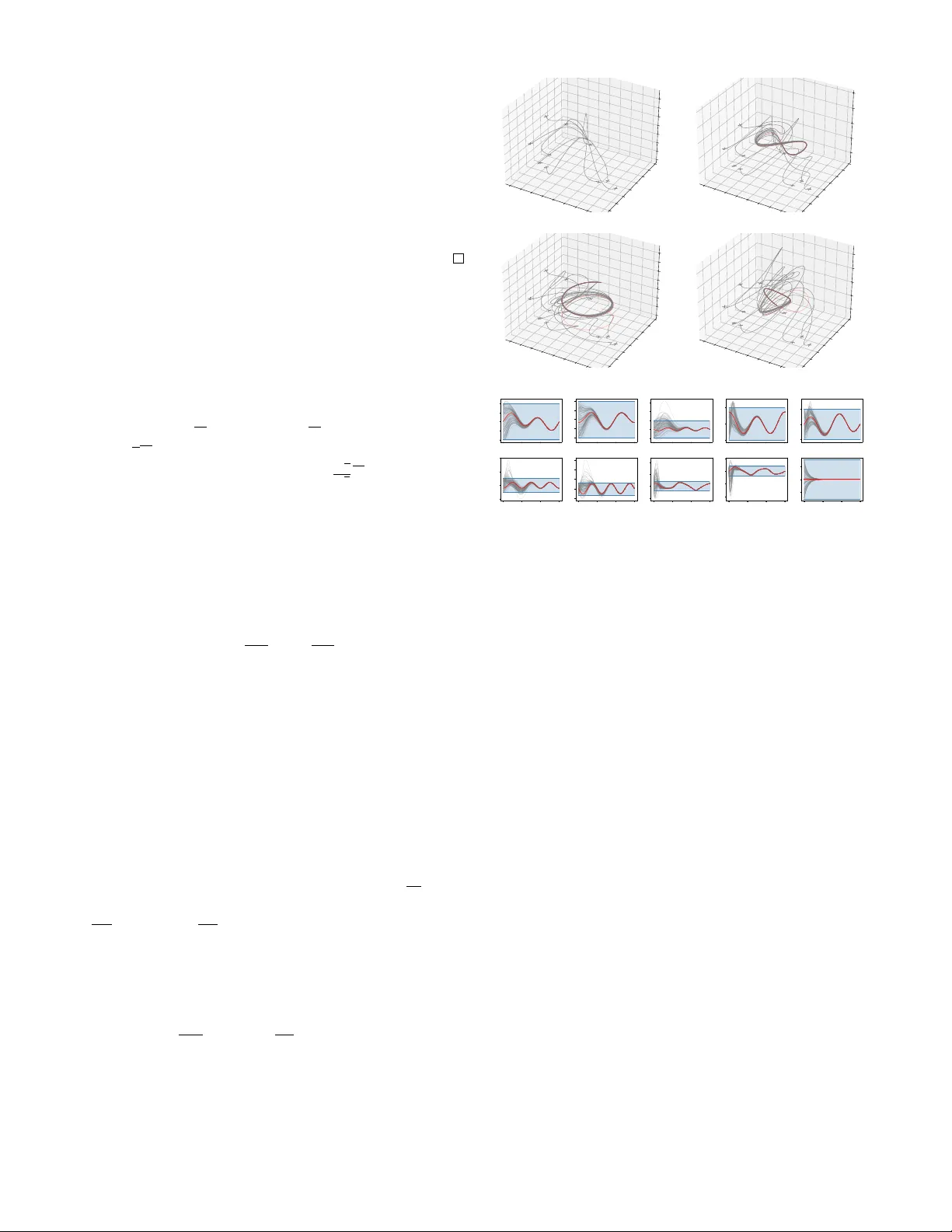
Learning Certified Neural Network Controllers Using Contraction and Interv al Analysis Akash Harapanahalli, Samuel Coogan, and Alexander Da vydo v Abstract — W e present a nov el framework that jointly trains a neural network contr oller and a neural Riemannian metric with rigorous closed-loop contraction guarantees using formal bound propagation. Dir ectly bounding the symmetric Rieman- nian contraction linear matrix inequality causes unnecessary over conservativeness due to poor dependency management. Instead, we analyze an asymmetric matrix function G , where 2 n GPU-parallelized cor ner checks of its interv al hull v erify that an entire interval subset X is a contraction region in a single shot. This eliminates the sample complexity problems encountered with pr evious Lipschitz-based guarantees. Additionally , f or control-affine systems under a Killing field assumption, our method produces an explicit tracking controller capable of exponentially stabilizing any dynamically feasible trajectory using just two forward inferences of the learned policy . Using J AX and immrax for linear bound propagation, we apply this approach to a full 10-state quadrotor model. In under 10 minutes of post-JIT training, we simultaneously learn a control policy π , a neural contraction metric Θ , and a verified 10- dimensional contraction region X . I . I N T R O D U C T I O N Learning-based methods hav e demonstrated potential for controlling complex nonlinear systems, o wing to their ability to represent and learn highly expressi ve policies that can be difficult to obtain through classical control design. Howe ver , deploying learned controllers in safety-critical applications demands rigorous guarantees on closed-loop behavior that such policies do not inherently provide. This gap between e xpressiv eness and certifiability has mo- tiv ated a growing body of work on formally verifying closed- loop beha vior of systems with neural network controllers. For instance, one can certify neural L yapunov functions for stabilization or neural control barrier functions for safety , using satisfiability modulo theory or branch-and-bound opti- mization to rigorously conclude the lack of counterexamples [1]. These exact verification approaches, howe ver , can be difficult to scale to large state spaces and deeper networks. A scalable alternative uses bound propa gation [2] to verify guaranteed ov erapproximations of the learned components. Beyond stabilization and in variance, contraction theory has provided a suite of tools suitable to tackle other chal- lenges like online tracking [3], and recent work has de- veloped neural contraction metrics [4] to help scale these methods. Howe ver , formally verifying the behavior of these contraction metrics remains a significant challenge, relying 1 Akash Harapanahalli and Samuel Coogan are with the School of Electrical and Computer Engineering, Georgia Institute of T echnology , Atlanta, GA, 30332, USA. { aharapan,sam.coogan } @gatech.edu 2 Alexander Da vydov is with the Department of Mechanical Engineering and Ken Kennedy Institute, Rice University , Houston, TX, 77005, USA. davydo v@rice.edu on Lipschitz-based sampling arguments or over -conservati ve bounding techniques [5], [6]. In this work, we use off-the- shelf neural network bound propagators, careful dependency management through the contraction condition, and an effi- cient exact characterization of the ℓ 2 -logarithmic norm of an interval matrix to jointly train neural network controllers and contraction metrics with formal guarantees. A. Pr oblem F ormulation and Contributions Consider a nonlinear control system of the form ˙ x = f ol ( t, x, u ) , (1) where x ∈ R n is the state of the system, u ∈ R m is a control input, and f ol : [0 , ∞ ) × R n × R m → R n is a C 1 smooth mapping. Our primary goal is to jointly synthesize an e xplicit feedback policy π ( x ) and a Riemannian metric M ( x ) such that the closed-loop system ˙ x = f π ( t, x ) := f ol ( t, x, π ( x )) (2) is contracting. W e also consider the special case of control- affine systems, ˙ x = f d ( x ) + g ( x ) u , where the goal extends to tracking any dynamically feasible trajectory . T o address these problems, we dev elop a no vel framework using bound propagation to jointly train a neural contraction metric and a neural network controller for nonlinear systems with formal guarantees of closed-loop contractivity . Our specific contributions are outlined: • Asymmetric Contraction Condition . W e propose an equiv alent asymmetric Riemannian contraction condition bounding the ℓ 2 -logarithmic norm of a matrix, directly in- volving the factored parameterization of the metric. While mathematically equiv alent on point-wise ev aluations, our asymmetric condition can dramatically reduce o verestima- tion error when using bound propagation tools due to better dependency management. • Certification and T raining via Bound Propagation . Using off-the-shelf bound propagators with automatic dif- ferentiation, we algorithmically obtain an interval hull of this asymmetric matrix. Applying a result from [7], we show how the maximum logarithmic norm within this interval hull can be checked with 2 n GPU parallelized corner checks. W e design a loss function in Algorithm 1 which, if nonpositi ve, certifies the contraction condition ov er an entire region X without exhaustiv e sampling. • Explicit T racking Control . In the special case where the system is control affine and the metric satisfies a Killing field condition (matching the strong CCM condition from [3, C2]), we propose a simple, explicit feedback controller u ( t, x ) = π ( x ) − π ( x ′ ( t )) + u ′ ( t ) , capable of tracking any dynamically feasible trajectory using only two forw ard inferences of the learned policy π . Notably , our method eliminates the need to search for a geodesic of the metric during online execution, and does not require any state augmentation into error coordinates. Finally , we demonstrate through a 10-state quadrotor bench- mark ho w the proposed method can certify and train explicit contracting tracking controllers, where sampling-based cer- tification would suffer from the curse of dimensionality . B. Backgr ound, Notation, and Related W ork Riemannian Metrics and Contraction Theory: Contrac- tion theory provides a geometric framework for translating infinitesimal linear properties into incremental exponential stability bounds between trajectories of the system. There is a rich literature in contraction analysis, including [8] for Riemannian spaces, [9] for a differential L yapunov function oriented framew ork, [10] for distances defined by possibly non-Euclidean norms, and [11], [3] for controller design. In this work, we focus on Riemannian geometry in R n . Let µ 2 ( · ) denote the induced ℓ 2 logarithmic norm µ 2 ( A ) = λ max ( A + A T 2 ) . For a matrix function A : R n → R n × n , let ∂ v A ( x ) = P n i =1 ∂ A ∂ x i ( x ) v i denote the directional deriv ativ e. Let X ⊆ R n be a set whose interior int X is nonempty and connected. A Riemannian metric M on X is a smooth, symmetric, positive-definite matrix function that is uniformly bounded , meaning there exist a, b > 0 such that aI ⪯ M ( x ) ⪯ bI for ev ery x ∈ X . M defines a length for piecewise-smooth paths γ : [0 , 1] → int X by integrating the Riemannian norm of the velocity: ℓ ( γ ) = R 1 0 p γ ′ ( s ) T M ( γ ( s )) γ ′ ( s )d s . This equips in t X with a distance d ( x, y ) , defined as the infimum of the lengths of all such paths in int X connecting x and y (we do not assume int X is geodesically complete, so this infimum may not be achieved by a geodesic within the space). Definition 1 (Contraction Region [8, Def. 2]) . A region of the state space X is called a contraction re gion of the v ector field f π from (2) with respect to metric M ( x ) if there exists c > 0 such that the linear matrix inequality S ( t, x ) ⪯ 0 holds uniformly ov er t ∈ [0 , ∞ ) , x ∈ X , where S ( t, x ) := M ( x ) ∂ f π ∂ x ( t, x ) + ∂ f π ∂ x ( t, x ) T M ( x ) + ∂ f π ( t,x ) M ( x ) + 2 cM ( x ) . (3) W e note that Definition 1 does not require X to be forward in variant. Definition 1 provides an important infinitesimal characterization of the follo wing property: if two trajectories contained within int X have a minimizing geodesic connect- ing them fully contained within int X , then d ( x ( t ) , y ( t )) ≤ e − ct d ( x (0) , y (0)) . This bound is useful in a number of contexts—for instance, for autonomous systems, if a contraction region is forward in variant, geodesically conv ex and complete, the flow map ϕ τ for fixed τ > 0 is a contraction mapping, and Banach’ s f ol Open-loop system (1) f π Closed-loop system (2) under policy u = π ( x ) f d Drift term for the control-affine system from (5) g Input vector fields for the control-affine system from (5) f cl Closed-loop system (8) under policy u = π ( x ) − π ( x ′ ) + u ′ X Region of the state space R n with nonempty interior in t X M Uniformly Riemannian metric o ver X Θ Upper triangular factorization satisfying M ( x ) = Θ( x ) T Θ( x ) d Metric geodesic distance associated to M π Feedback policy S Left-hand side of the contraction LMI (3) G Asymmetric contraction matrix from Definition 2 T ABLE I: Symbols and Notation fixed point theorem concludes that the system exponentially con verges to a unique equilibrium. Interval Analysis and Bound Pr opagation: Let IR de- note the set of closed intervals of R , of the form [ a, a ] := { a ∈ R : a ≤ a ≤ a } for a, a ∈ R . An interval matrix [ A ] = [ A, A ] ∈ IR m × n is a matrix where [ A ] ij = [ A ij , A ij ] ∈ IR . [ A ] is a subset of R m × n in the entrywise sense, so A ∈ [ A ] if A ij ∈ [ A ] ij for e very i = 1 , . . . , m and j = 1 , . . . , n . For the interv al matrix [ A ] , we notate its center A c ∈ R m × n as A c =  A + A  / 2 and its radius A ∆ ∈ R m × n as A ∆ =  A − A  / 2 . Giv en a matrix function A : R n → R m × n , an interval hull of A over an input set X ⊆ R n is an interval matrix [ A ] ∈ R m × n such that A ( x ) ∈ [ A ] uniformly for ev ery x ∈ X . Obtaining the smallest interval hull of A is generally an intractable noncon vex optimization problem. Instead, a general way to obtain larger valid interval hulls is through bound pr opagation , where (i) a computation tree for A is built through an abstract e valuation, and (ii) the input bound X is successiv ely propagated through the computation tree. These existing approaches ha ve varying tradeof fs of accuracy and runtime: interv al bound propagation [12], [13], which efficiently propagates lo wer and upper scalar bounds; linear bound propagation [14], which propagates linear lower and upper bounding functions; set-based methods [15] including zonotopes and star sets [16], which propagate set ov erap- proximations forward through the network; T aylor models [17] and other polynomial approximators, which propagate tighter but more computationally expensi ve representations. A fundamental issue often encountered by these various approaches is the dependency pr oblem . When a v ariable x appears multiple times in a computation graph, these methods often treat each instance as an independent v ariable, failing to capture algebraic interactions between terms. W e demonstrate this phenomenon in Example 1 in the next Section, and sho w how our asymmetric formulation mitigates these issues. I I . R I E M A N N I A N C O N T R AC T I O N V I A B O U N D P R O PAG A T I O N In prior contraction synthesis works [4], the LMI (3) is in- corporated into the training by sampling points x n across the desired contraction region X and backpropagating against λ max ( S ( t, x n )) . In this section, we use bound propagation to directly verify the contraction condition over the region X without sampling, which we use to design an explicit tracking control policy for control-affine systems. A. The Asymmetric Contraction Matrix W e first propose an asymmetric matrix that reduces the ov erestimation error from bound propagation. Definition 2 (Asymmetric Contraction Matrix) . Consider the vector field f π from (2), a Riemannian metric M ( x ) = Θ( x ) T Θ( x ) , and a fixed c > 0 . Define the asymmetric contraction matrix as the following: G ( t, x ) := Θ( x ) T  ∂ f π ( t,x ) Θ( x ) + Θ( x )  ∂ f π ∂ x ( t, x ) + cI  . (4) The follo wing lemma demonstrates how an ℓ 2 -logarithmic norm bound on G is equiv alent to the LMI (3), building off the fact that the symmetrization of G matches S (up to a factor of 2). Lemma 1 (Equiv alence) . Consider the vector field f π fr om (2) , let M ( x ) = Θ( x ) T Θ( x ) be a Riemannian metric, and c > 0 be fixed. The following are equivalent: (i) S ( t, x ) ⪯ 0 , with S defined as the LHS of the LMI (3) ; (ii) µ 2 ( G ( t, x )) ≤ 0 , with G defined as the asymmetric contraction matrix (4) . Thus, X is a contraction r e gion if and only if µ 2 ( G ( t, x )) ≤ 0 uniformly over t ∈ [0 , ∞ ) , x ∈ X . Pr oof. Expanding G and adding its transpose re veals G ( t, x ) + G ( t, x ) T = 2 c Θ( x ) T Θ( x ) + Θ( x ) T ∂ f π ( t,x ) Θ( x ) +  ∂ f π ( t,x ) Θ( x )  T Θ( x ) + Θ( x ) T Θ( x ) ∂ f π ∂ x ( t, x ) + ∂ f π ∂ x ( t, x ) T Θ( x ) T Θ( x ) . Substituting M ( x ) = Θ( x ) T Θ( x ) and ∂ f π ( x ) M ( x ) =  ∂ f π ( x ) Θ( x )  T Θ( x ) + Θ( x ) T ∂ f π ( x ) Θ( x ) using the standard matrix product rule shows that S ( t, x ) = G ( t, x ) + G ( t, x ) T . Thus, µ 2 ( G ( t, x )) = λ max  S ( t,x ) 2  is nonpositive if and only if S ( t, x ) has all nonpositive eigen values. W e note that the condition µ 2 ( G ( t, x )) ≤ 0 is different from the condition µ 2 ( F ( t, x )) ≤ − c provided in [8, Def. 2], which bounds the logarithmic norm of the generalized J a- cobian F ( t, x ) =  ∂ f π ( t,x ) Θ( x ) + Θ( x ) ∂ f π ∂ x ( t, x )  Θ( x ) − 1 . Bounding F would require propagating bounds through a matrix in version, which is difficult. Instead, the asymmetric contraction matrix (4) requires only a transpose of Θ . The follo wing analytical e xample demonstrates how while the two conditions are theoretically equiv alent, applying bound propagation strategies to G ( t, x ) instead of S ( t, x ) can dramatically reduce o verestimation error due to lost information in the symmetrization. Example 1 (Dependency management) . In the scalar case, we can easily compare the expressions (3) and (4), S = Θ 2 J + J Θ 2 + Θ ˙ Θ + ˙ ΘΘ + 2 c Θ 2 , G = Θ( ˙ Θ + Θ( J + c )) . Of course, while S = 2 G analytically , recall from Sec- tion I-B that bound propagators like interv al analysis and CR OWN directly trace the above expressions into compu- tation graphs—and the distinction between bounding S and G can become significant. The expression for G captures interactions between ˙ Θ and Θ J before premultiplying by Θ , while the expression for S multiplies before adding. For instance, e valuation of the above e xpressions over Θ ∈ [0 . 5 , 1] , ˙ Θ ∈ [ − 2 , − 1 . 5] , J ∈ [ − 1 , 1] and c = 0 . 5 giv es S ∈ [ − 5 . 75 , 1 . 5] and 2 G ∈ [ − 5 , 0] , which is a significant difference when trying to verify nonpositivity (contraction) using Lemma 1. B. Efficient P arallel Corner Checks Giv en an interv al matrix [ A ] , one way to solve max A ∈ [ A ] µ 2 ( A ) is to (i) write [ A ] = co { A k } 2 n 2 k =1 ( co is the con vex hull), where the A k consist of all 2 n 2 matrices of the form ( A k ) ij ∈ { A ij , A ij } , and (ii) note that µ 2 is conv ex, so max A ∈ [ A ] µ 2 ( A ) = max k ∈{ 1 ,..., 2 n 2 } µ 2 ( A k ) . While this exactly computes the largest logarithmic norm of the set, it scales very poorly in n . Instead, we apply a result from [7] to reduce the number of corner checks down to 2 n . For the n = 10 quadrotor in Section IV, for instance, 2 10 2 is over 10 30 corners, while 2 10 is far more practical at 1024 corners. Lemma 2 ([7, Thm 1]) . F or an interval matrix [ A ] ∈ IR n × n , max A ∈ [ A ] µ 2 ( A ) = max  µ 2 ( A c + diag( s ) A ∆ diag( s )) : s ∈ {− 1 , +1 } n  . The proof is in [7] in the context of verifying the positiv e definiteness of an interv al matrix—we make slight modifica- tions to bound the function µ 2 ( A ) = λ max ( A + A T 2 ) instead. Pr oof. W e first recall that µ 2 ( A ) = max v : | v | 2 =1 ( v T A + A T 2 v ) = max v : | v | 2 =1 v T Av . Let A ∈ [ A ] . W e can write v T Av = v T A c v + v T ( A − A c ) v . Then, since | v T ( A − A c ) v | ≤ | v | T | A − A c || v | ≤ | v | T A ∆ | v | , where | · | is the entrywise absolute value, we hav e v T Av ≤ v T A c v + | v | T A ∆ | v | . Define a sign vector s ( v ) ∈ {− 1 , +1 } n by ( s ( v )) j = sign( v j ) —then | v | = diag ( s ) v and v T Av ≤ v T A c v + v T diag( s ( v )) A ∆ diag( s ( v )) v = v T ( A c + diag( s ( v )) A ∆ diag( s ( v ))) v ≤ max { v T ( A c + diag( s ) A ∆ diag( s )) v : s ∈ {− 1 , +1 } n } . T aking a max ov er v with | v | 2 = 1 on either side and swapping the order of max , µ 2 ( A ) ≤ µ 2 ( A c + diag( s ) A ∆ diag( s )) for some sign vector s . The containment A c + diag( s ) A ∆ diag( s ) ∈ [ A ] implies equality . Algorithm 1 Certified Neural Contraction Metric Losses 1: Input : a, b > 0 metric bounds, c ≥ 0 contraction rate 2: function L O S S ( Θ , π ; X , a, b, c ) 3: [ G ] ← interval hull of G from Definition 2 over X 4: λ ← max s ∈{− 1 , +1 } n µ 2 ( G c + diag( s ) G ∆ diag( s )) 5: [ M ] ← interval hull of Θ T Θ ov er X 6: ˆ a ← min s ∈{− 1 , +1 } n − µ 2 ( − M c + diag( s ) M ∆ diag( s )) 7: ˆ b ← max s ∈{− 1 , +1 } n µ 2 ( M c + diag( s ) M ∆ diag( s )) 8: retur n max { λ, 0 } + max { a − ˆ a, 0 } + max { ˆ b − b, 0 } Remark 1 . In prior work [6], a sufficient condition to check the negativ e (semi-)definiteness of an interval matrix [ A ] constructs a matrix B bounding the Metzler majorant ⌈ A ⌉ Mzr 1 of any matrix A ∈ [ A ] , and verifies that this matrix has all eigen values with negati ve real part. Howe ver , this suf ficient condition is inherently conserv ativ e, even for single matrices. For example, A = − tv v T with t > 0 and v = [1 , . . . , 1] T ∈ R n is negati ve semidefinite yet its Metzler majorant has maximum eigenv alue equal to t ( n − 2) which is positi ve for all n > 2 and grows unbounded as t → ∞ . Applying Lemma 2 with an interv al hull of the asymmetric contraction matrix ov er a region X , we can verify that X is a contraction region through 2 n corner checks. Theorem 1. Let [ G ] ∈ IR n × n be an interval hull of the asymmetric contraction matrix G from (4) over [0 , ∞ ) × X , for fixed c > 0 and re gion X ⊆ R n . If max  µ 2 ( G c + diag( s ) G ∆ diag( s )) : s ∈ {− 1 , +1 } n  ≤ 0 , then X is a contraction re gion for the nonlinear system f π fr om (2) at rate c . Pr oof. Lemma 2 implies max x ∈ X µ 2 ( G ( t, x )) ≤ 0 , and Lemma 1 completes the proof. C. Loss for Certified Metric and P olicy T raining In Algorithm 1, we propose a loss to jointly train the policy π and the metric Θ T Θ . Corollary 1. If L O S S (Θ , π ; X, a, b, c ) ≤ 0 in Algorithm 1, for a, b, c > 0 , then (i) M ( x ) = Θ( x ) T Θ( x ) satisfies aI ⪯ M ( x ) ⪯ bI , and (ii) X is a contraction r e gion for the closed-loop system ˙ x = f π ( x ) = f ol ( x, π ( x )) fr om (2) at rate c . Pr oof. L O S S (Θ , π ; X, a, b, c ) ≤ 0 implies λ ≤ 0 , a − ˆ a ≤ 0 and ˆ b − b ≤ 0 . By Lemma 2, for every M ∈ [ M ] , ˆ a ≤ λ min (( M + M T ) / 2) 2 and λ max (( M + M T ) / 2) ≤ ˆ b implying part (i). Part (ii) follows by application of Theorem 1. A crucial step in our algorithm is obtaining the interval hulls [ G ] and [ M ] containing the output of (4) ov er an input set X . In practice, we found that linear bound propagation in 1  ⌈ A ⌉ Mzr  ij = | A ij | if i  = j and  ⌈ A ⌉ Mzr  ii = A ii . 2 Since − µ 2 ( − A ) = − λ max ( − A − A T 2 ) = λ min ( A + A T 2 ). the style of CR O WN [14], [18] provided the right balance of accuracy , scalability , and trainability . W e use the implemen- tation provided in our toolbox immrax [19] 3 in J AX [20]. J AX allo ws us to automatically (i) construct the asymmetric contraction matrix (4) using automatic dif ferentiation, (ii) trace the computation graph applying linear bound propa- gation, and (iii) backpropagate the loss from Algorithm 1 and dispatch the neural network training to the GPU. I I I . E X P L I C I T T R A C K I N G C O N T RO L D E S I G N Consider the following control-affine nonlinear system, ˙ x = f ol ( x, u ) = f d ( x ) + g ( x ) u, (5) where f d : R n → R n is a C 1 drift term and g ( x ) ∈ R n × m is a C 1 state dependent matrix. W ith some restrictions on the choice of metric M ( x ) , we can apply the methodology from the previous section to design a simple feedback controller to exponentially track any dynamically feasible trajectory within the contraction region X . Notably , we do not require any online geodesic computations like [3], [21], or any state space augmentation with the trajectory to be tracked like previous learning-based methods [4]. Corollary 2. Suppose L O S S (Θ , π ; X , a, b, c ) ≤ 0 for the nonlinear system ˙ x = f d ( x ) + g ( x ) u with hyperparameters a, b, c > 0 , satisfying the following condition: for every j = 1 , . . . , m and every x ∈ X , ∂ g j ( x ) Θ( x ) + Θ( x ) ∂ g j ∂ x ( x ) = 0 . (6) Let x ′ ( t ) be a trajectory associated with a nominal input curve u ′ ( t ) . If ther e exists an R > 0 such that the metric tube of radius R ar ound x ′ ( t ) is fully contained inside int X , i.e. , for every t ≥ 0 , { x : d ( x, x ′ ( t )) ≤ R } ⊆ int X , then any trajectory x ( t ) under the feedback policy u ( t, x ) = π ( x ) − π ( x ′ ( t )) + u ′ ( t ) (7) with initial condition d ( x (0) , x ′ (0)) ≤ R satisfies d ( x ( t ) , x ′ ( t )) ≤ e − ct d ( x (0) , x ′ (0)) , for every t ≥ 0 . Pr oof. Letting v ( t ) = u ′ ( t ) − π ( x ′ ( t )) , and f π ( t, x ) = f d ( x ) + g ( x ) π ( x ) , the closed-loop dynamics are ˙ x = f cl ( t, x ) = f π ( t, x ) + P m j =1 g j ( x ) v j ( t ) . (8) Computing the asymmetric contraction matrix from Defini- tion 2, by linearity , for t ∈ [0 , ∞ ) , x ∈ X , G cl ( t, x ) = G π ( t, x ) + Θ( x ) T  P m j =1  ∂ g j ( x ) Θ( x ) + Θ( x ) ∂ g j ∂ x ( x )  v j ( t )  , where G π ( t, x ) = Θ( x ) T  ∂ f π ( t,x ) Θ( x ) + Θ( x )  ∂ f π ∂ x ( t, x ) + cI  is the asymmetric contraction matrix of f π . The con- dition L O S S (Θ , π ; X, a, b, c ) ≤ 0 implies that we ha ve µ 2 ( G π ( t, x )) ≤ 0 by Corollary 1. By assumption (6), the second term vanishes. Thus, subadditivity of µ 2 ( · ) implies 3 https://github.com/gtfactslab/immrax µ 2 ( G cl ( t, x )) ≤ µ 2 ( G π ( t, x )) + µ 2 (0) ≤ 0 . Therefore, Lemma 1 implies X is a contraction region for the closed- loop system f cl (8) at rate c . T o conclude, since u ( t, x ′ ( t )) = u ′ ( t ) , the uniqueness of solutions implies x ′ ( t ) is the trajectory of f cl from initial condition x ′ (0) . Because x ′ is a trajectory of a contracting system with a metric tube of radius R around it contained in the open and connected set int X , there is a minimizing geodesic between x and x ′ contained in int X which shrinks exponentially at rate c [8, Thm 1]. Remark 2 (Geodesic metric tube) . The tube of radius R in Corollary 2 is analytically important, ensuring geodesic paths connecting the two trajectories are alw ays contained within the contraction region. Howe ver , computationally finding such suble vel sets of the geodesic metric is difficult due to the need to search for geodesics. For simpler guarantees, one could apply the uniform bounds on the metric to obtain ℓ 2 -ball tubes sandwiching a geodesic metric tube: if { x : ∥ x − x ′ ( t ) ∥ 2 ≤ R } ⊆ int X for R > 0 , then the radius R = √ aR geodesic metric ball is also contained in int X , and points satisfying ∥ x − x ′ (0) ∥ 2 ≤ √ a √ b R liv e within the radius R ball at time 0 . In practice, we find that controllers trained to satisfy the contraction condition within region X hav e good beha vior when geodesics and e ven the trajectories themselves leave X (see Section IV). Remark 3 (Killing field condition) . The condition (6) e xactly matches the strong CCM condition [3, C2] which requires the actuation vector fields g j to be Killing fields of the metric, ∂ g j ( x ) M ( x ) + M ( x ) ∂ g j ∂ x ( x ) + ∂ g j ∂ x ( x ) T M ( x ) = 0 , which follo ws by a similar computation as Lemma 1. Enforcing this constraint on the neural network Θ is generally challenging. Howe ver , for systems with a constant g ( x ) = B for B ∈ R n × m , we can augment the neural network with a linear layer projecting x into the orthogonal subspace to B , using a matrix B ⊥ satisfying B ⊥ B = 0 . For instance, when B = [0 , I ] T , restricting the argument of Θ to the first n − m components of x structurally satisfies (6). Remark 4 (Control contraction metrics (CCM) and complete integrability) . Follo wing the discussion in [3, p. 3], our learned metric M ( x ) = Θ( x ) T Θ( x ) and policy π provide a completely inte grable differential control la w δ u = ∂ π ∂ x ( x ) δ x , which exponentially stabilizes the variational dynamics ˙ δ x = ( ∂ f d ∂ x ( x ) + P m j =1 ∂ g j ∂ x ( x ) u ′ j ) δ x + g ( x ) δ u , along trajectories ( x ′ , u ′ ) . This can be seen by ev aluating LMI (3) directly on the closed-loop dynamics f cl (8), and simplifying the result- ing expression using the Killing field condition discussed in Remark 3 to obtain the following: M ( x )  ∂ f d ∂ x ( x ) + g ( x ) ∂ π ∂ x ( x )  + ( ⋆ ) T M ( x ) + ∂ f d ( x )+ g ( x ) π ( x ) M ( x ) + 2 cM ( x ) ⪯ 0 , which verifies the quadratic (Finsler-)L yapunov condition on V ( x, δ x ) = δx T M ( x ) δ x . In contrast, the con vex criteria from control contraction metrics (CCM) [3] instead require − 10 . 0 − 7 . 5 − 5 . 0 − 2 . 5 0 . 0 2 . 5 5 . 0 7 . 5 10 . 0 p x − 10 . 0 − 7 . 5 − 5 . 0 − 2 . 5 0 . 0 2 . 5 5 . 0 7 . 5 p y − 7 . 5 − 5 . 0 − 2 . 5 0 . 0 2 . 5 5 . 0 7 . 5 10 . 0 p z (a) Hover − 10 . 0 − 7 . 5 − 5 . 0 − 2 . 5 0 . 0 2 . 5 5 . 0 7 . 5 10 . 0 p x − 10 . 0 − 7 . 5 − 5 . 0 − 2 . 5 0 . 0 2 . 5 5 . 0 7 . 5 p y − 5 0 5 10 15 p z (b) Figure Eight − 10 . 0 − 7 . 5 − 5 . 0 − 2 . 5 0 . 0 2 . 5 5 . 0 7 . 5 10 . 0 p x − 10 . 0 − 7 . 5 − 5 . 0 − 2 . 5 0 . 0 2 . 5 5 . 0 7 . 5 p y − 7 . 5 − 5 . 0 − 2 . 5 0 . 0 2 . 5 5 . 0 7 . 5 10 . 0 p z (c) Helix − 10 . 0 − 7 . 5 − 5 . 0 − 2 . 5 0 . 0 2 . 5 5 . 0 7 . 5 10 . 0 p x − 10 . 0 − 7 . 5 − 5 . 0 − 2 . 5 0 . 0 2 . 5 5 . 0 7 . 5 p y − 5 0 5 10 15 p z (d) Trefoil Knot t − 10 − 5 0 5 10 p x t − 10 − 5 0 5 10 p y t − 10 0 10 20 30 p z t − 5 0 5 ˙ p x t − 5 0 5 ˙ p y 0 5 10 15 t − 10 0 10 20 ˙ p z 0 5 10 15 t 5 10 15 20 25 f 0 5 10 15 t − 1 0 1 2 φ 0 5 10 15 t − 2 − 1 0 1 θ 0 5 10 15 t − 1 0 1 ψ (e) States vs Time for T refoil Knot Fig. 1: Plots (a)-(d) demonstrate how 10 randomly sampled initial conditions (pictured with the × ) sampled in the verified contraction region X stabilize to the nominal trajectories pictured in red under the tracking policy from Corollary 2. Plot (e) shows the state vs time for 100 randomly sampled initial conditions starting in X for the trefoil knot (d). The nominal trajectory is in red, with the verified contraction region X in blue. While some trajectories leav e the verified region, the controller empirically behav es well, bringing them back into the region and stabilizing to the commanded trajectory . only a path inte grable dif ferential controller δu = K ( t, x ) δx , where K may not be the Jacobian of an explicit function. This comes at the cost of an implicit control policy , which requires an online search for a geodesic path between the current state and the reference. Instead, our controller pro- vides an explicit representation, where two simple forward inferences of the policy π provide the control input at minimal computational cost. I V . E X A M P L E : C O N T R AC T I N G T R A C K I N G C O N T RO L F O R 1 0 S TA T E Q UA D RO T O R In this section, we apply the methodology from the pre- vious section to design a contracting tracking controller for the 10-state quadrotor from [21], 4 ¨ p x = − τ sin θ, (9a) ¨ p y = τ cos θ sin ϕ, (9b) ¨ p z = g − τ cos θ cos ϕ, (9c) where x = [ p x , p y , p z , ˙ p x , ˙ p y , ˙ p z , τ , ϕ, θ, ψ ] T , for displace- ment [ p x , p y , p z ] T ∈ R 3 in North-East-Down con vention, [ ϕ, θ , ψ ] T ∈ R 3 the XYZ Euler-angle representation, τ ∈ R 4 The code reproducing the results is available at https://github.com/gtfactslab/neural_contraction the net (mass-normalized) thrust, and u = [ ˙ τ , ˙ ϕ, ˙ θ , ˙ ψ ] T is the control input. T o warm start the learning process, we first linearize the dynamics around the equilibrium hover point x eq = [0 , . . . , 0 , g , 0 , 0 , 0] T , u eq = [0 , 0 , 0 , 0] T , and use LQR to obtain a pair ( K , S ) , where K is the linear controller and S is the solution to the Ricatti equation. Then, given neural networks Θ res , π res , we set Θ( x ) = cholesky ( S ) T + Θ res ( x ) and π ( x ) = K ( x − x eq ) + u eq + π res ( x ) . For the residual networks themselves, we use zero-initialized MLPs both with 2 hidden layers of 128 neurons each. Θ res first projects the state onto the first 6 components, then maps to n ( n + 1) / 2 = 55 outputs populating the upper triangle of an 10 × 10 matrix, and π res maps the state to the 4 control outputs. Since the learned networks need to be smooth, we use softplus ( σ ( x ) = log(1 + e x ) ) acti vations. W e trained the following contraction region X = [ − 10 , 10] 3 × [ − 5 , 5] 3 × [ 2 g 3 , 4 g 3 ] × [ − π 8 , π 8 ] 2 × [ − π 2 , π 2 ] optimizing o ver gro wing regions n 100 X , where we checkpoint and iterate n when the loss hits 0 until n = 100 . W e partition each n -th region uniformly into 9 3 = 729 partitions ov er the ( τ , ϕ, θ ) states.729 W e use the AdamW optimizer with the loss from Algorithm 1, with a = 0 . 01 , b = 100 , c = 0 . 001 . In total, the training took a total of 1415 steps in 736 seconds, including 164 seconds for JIT compilation. 5 W e use the dif ferential flatness property of quadrotor dynamics to extract a dynamically feasible pair ( x ′ ( t ) , u ′ ( t )) based on a desired C 3 curve [ p ′ x ( t ) , p ′ y ( t ) , p ′ z ( t ) , ψ ′ ( t )] T . Then, we apply the explicit feedback policy deri ved in Corollary 2 to track this trajectory . Compared to [4], we get a formal guarantee of contraction over the whole region X , which was intractible with sampling-based guarantees for n = 10 , and we completely av oid the need to search for minimizing geodesics like the approach from [21]. V . C O N C L U S I O N A N D F U T U R E W O R K In this letter , we presented a framew ork for jointly learning a neural network controller and a neural contraction metric with formal guarantees of closed-loop contraction over a region X . By lev eraging (i) a novel asymmetric contraction condition and (ii) interval analysis with GPU-parallelized corner checks, our approach a voids the conservatism of direct LMI bounding and sample complexity issues associated to Lipschitz-based guarantees. For control-affine systems satisfying a Killing field condition, we provided an explicit tracking controller requiring only two forward inferences of the network. W e demonstrated the approach on a 10-state quadrotor . Sev eral directions remain for future work. Incorporating forward in variance guarantees for the certified region and enforcing bounded control inputs would strengthen the prac- tical applicability of the framew ork. More broadly , e xtending the approach to learn Finsler-L yapuno v functions or to certify 5 Code was run on a desktop running Kubuntu 22.04, with AMD Ryzen 5 5600X, NVIDIA R TX 3070, and 32 GB of RAM. contraction with respect to non-Euclidean norms could fur- ther expand its scope to systems where Riemannian metrics are not the most natural choice. R E F E R E N C E S [1] A. Abate, D. Ahmed, M. Giacobbe, and A. Peruffo, “Formal synthesis of Lyapuno v neural networks, ” IEEE Contr ol Systems Letters , vol. 5, no. 3, pp. 773–778, 2021. [2] C. Liu, T . Arnon, C. Lazarus, C. Strong, C. Barrett, and M. J. Kochen- derfer , “ Algorithms for verifying deep neural networks, ” F oundations and Tr ends in Optimization , vol. 4, no. 3-4, pp. 244–404, 2021. [3] I. R. Manchester and J.-J. E. Slotine, “Control contraction metrics: Con vex and intrinsic criteria for nonlinear feedback design, ” IEEE T ransactions on Automatic Control , vol. 62, no. 6, pp. 3046–3053, 2017. [4] D. Sun, S. Jha, and C. Fan, “Learning certified control using con- traction metric, ” in Conference on Robot Learning , pp. 1519–1539, PMLR, 2021. [5] M. Zakwan, L. Xu, and G. Ferrari-T recate, “Neural exponential stabilization of control-affine nonlinear systems, ” in IEEE Conference on Decision and Contr ol (CDC) , pp. 8602–8607, 2024. [6] A. Davydov , “V erifying closed-loop contractivity of learning-based controllers via partitioning, ” arXiv preprint , 2025. [7] J. Rohn, “Positi ve definiteness and stability of interval matrices, ” SIAM Journal on Matrix Analysis and Applications , vol. 15, no. 1, pp. 175– 184, 1994. [8] W . Lohmiller and J.-J. E. Slotine, “On contraction analysis for non- linear systems, ” Automatica , v ol. 34, no. 6, pp. 683–696, 1998. [9] F . Forni and R. Sepulchre, “ A differential L yapunov framework for contraction analysis, ” IEEE Tr ansactions on Automatic Control , vol. 59, no. 3, pp. 614–628, 2013. [10] A. Davydov , S. Jafarpour, and F . Bullo, “Non-Euclidean contraction theory for robust nonlinear stability , ” IEEE T ransactions on Automatic Contr ol , vol. 67, no. 12, pp. 6667–6681, 2022. [11] E. D. Sontag, “Contractiv e systems with inputs, ” in P erspectives in Mathematical System Theory , Contr ol, and Signal Processing: A F estschrift in Honor of Y utaka Y amamoto on the Occasion of his 60th Birthday , pp. 217–228, Springer , 2010. [12] L. Jaulin, M. Kieffer , O. Didrit, and E. W alter , Applied Interval Analysis . Springer, 1st edition. ed., 2001. [13] S. Gowal, K. Dvijotham, R. Stanforth, R. Bunel, C. Qin, J. Uesato, R. Arandjelovic, T . Mann, and P . Kohli, “On the effectiv eness of interval bound propagation for training verifiably robust models, ” arXiv preprint arXiv:1810.12715 , 2018. [14] H. Zhang, T .-W . W eng, P .-Y . Chen, C.-J. Hsieh, and L. Daniel, “Efficient neural network rob ustness certification with general activ a- tion functions, ” Advances in Neural Information Pr ocessing Systems , vol. 31, 2018. [15] M. Althoff, G. Frehse, and A. Girard, “Set propagation techniques for reachability analysis, ” Annual Review of Control, Robotics, and Autonomous Systems , v ol. 4, no. 1, pp. 369–395, 2021. [16] H.-D. T ran, D. Manzanas Lopez, P . Musau, X. Y ang, L. V . Nguyen, W . Xiang, and T . T . Johnson, “Star-based reachability analysis of deep neural networks, ” in International symposium on formal methods , pp. 670–686, Springer , 2019. [17] X. Chen, Reachability Analysis of Non-Linear Hybrid Systems Using Taylor models . PhD Thesis, Fachgruppe Informatik, R WTH Aachen Univ ersity , 2015. [18] K. Xu, Z. Shi, H. Zhang, Y . W ang, K.-W . Chang, M. Huang, B. Kailkhura, X. Lin, and C.-J. Hsieh, “ Automatic perturbation analy- sis for scalable certified robustness and beyond, ” Advances in Neural Information Processing Systems , vol. 33, pp. 1129–1141, 2020. [19] A. Harapanahalli, S. Jafarpour , and S. Coogan, “immrax: A paral- lelizable and differentiable toolbox for interval analysis and mixed monotone reachability in J AX, ” IF AC-P apersOnLine , vol. 58, no. 11, pp. 75–80, 2024. [20] J. Bradbury , R. Frostig, P . Hawkins, M. J. Johnson, C. Leary , D. Maclaurin, G. Necula, A. Paszke, J. V anderPlas, S. W anderman- Milne, and Q. Zhang, “J AX: composable transformations of Python+NumPy programs, ” 2018. [21] S. Singh, B. Landry , A. Majumdar , J.-J. Slotine, and M. Pav one, “Robust feedback motion planning via contraction theory , ” The In- ternational Journal of Robotics Resear ch , vol. 42, no. 9, pp. 655–688, 2023.