Tightening CVaR Approximations via Scenario-Wise Scaling for Chance-Constrained Programming

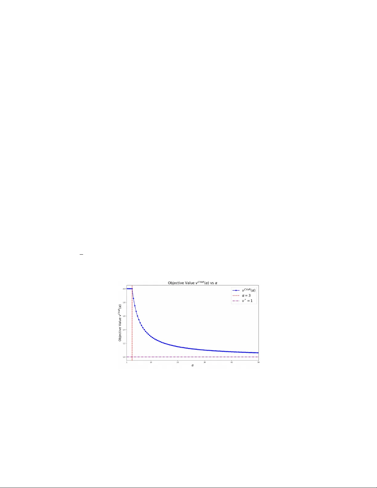
Tigh tening CV aR Appro ximations via Scenario-Wise Scaling for Chance-Constrained Programming Nan Jiang 1 , Rui Chen 2 1 The Hong Kong Univ ersity of Science and T echnology (nanjiang@ust.hk) 2 The Chinese Univ ersity of Hong Kong, Shenzhen (rc hen@cuhk.edu.cn) Marc h 31, 2026 Abstract Chance-constrained programs (CCPs) pro vide a p o werful modeling framework for decision- making under uncertain ty , but their noncon vex feasible regions mak e them computationally c hallenging. A widely used conv ex inner appro ximation replaces chance constraints with Con- ditional V alue-at-Risk (CV aR) constraints; ho wev er, the resulting solutions can b e ov erly con- serv ativ e and sub optimal. W e propose a scenario-wise scaling approach that strengthens CV aR appro ximations for CCPs with ﬁnitely supp orted uncertaint y . The metho d introduces scal- ing factors that reweigh t individual scenarios within the CV aR constraint, yielding a family of p oten tially tighter inner approximations. W e establish suﬃcient conditions under which, for a suitable choice of scaling factors, the scaled CV aR appro ximation attains the same op- timal v alue as the original CCP and admits a (near-)optimal solution of the CCP . W e show that these conditions are tight and further relax them in the conv ex setting. W e also show that optimizing ov er scenario-wise scaling factors is NP-hard. T o address this computational c hallenge, w e develop eﬃcien t heuristic and sequen tial conv ex approximation algorithms that iterativ ely update the scaling factors and generate impro ved feasible solutions. Numerical ex- p erimen ts demonstrate that the prop osed metho ds consistently improv e up on standard CV aR and state-of-the-art conv ex appro ximations, often reducing conserv ativ eness while maintaining tractabilit y . 1 In tro duction Chance-constrained programs (CCPs) provide a principled wa y to optimize decisions under uncer- tain ty by explicitly controlling the probability of constraint violation. Speciﬁcally , a CCP c ho oses a decision x ∈ X ⊆ R n to minimize (without loss of generality) a linear cost sub ject to the requiremen t that some uncertain constrain t holds with high probability: v ∗ = min x ∈X n c ⊤ x : P n ˜ ξ : g ( x , ˜ ξ ) ≤ 0 o ≥ 1 − ε o , (1) where ˜ ξ is a random v ector, g ( · , · ) mo dels the uncertain feasibility constraint, and ε ∈ (0 , 1) is a risk tolerance. Throughout this pap er, we assume that CCP (1) is feasible, and the uncertaint y is ﬁnitely supp orted, as speciﬁed below. Assumption 1. The underlying pr ob ability distribution of ˜ ξ is ﬁnite, i.e. ˜ ξ has N p ossible r e al- izations (i.e., sc enarios) { ξ 1 , ξ 2 , · · · , ξ N } with p i = P { ˜ ξ = ξ i } for i ∈ [ N ] , and P i ∈ [ N ] p i = 1 . 1 This assumption is common in the CCP literature (see, e.g., [28, 24, 33, 3]), as one can often appro ximate a general distribution using a ﬁnite sample. With the ﬁnitely supported distribution P , we can equiv alen tly rewrite CCP (1) as v ∗ = min x ∈X    c ⊤ x : X i ∈ [ N ] p i I  g ( x , ξ i ) ≤ 0  ≥ 1 − ε    , (2) where I [ · ] is the zero-one indicator function. Without loss of generality , we assume that the function g ( x , ξ ) is deﬁned as g ( x , ξ ) = max j ∈ [ J ] g j ( x , ξ ), where g j ( x , ξ ) : R n × Ξ → R for all j ∈ [ J ] := { 1 , . . . , J } . Therefore, form ulation (2) can model both single and joint chance-constrained programs. When J = 1, CCP (2) includes a single chance con- strain t; otherwise, it con tains a joint c hance constrain t where g ( x , ξ i ) ≤ 0 if and only if g j ( x , ξ i ) ≤ 0 for each j ∈ [ J ]. 1.1 Motiv ation Despite its mo deling pow er, CCP (2) is computationally challenging: even with linear g ( · , ξ ) and X = R n + , the problem is NP-hard [28]. As a result, a large b ody of work dev elops conv ex ap- pro ximations of (2). A conv enien t w ay to express the chance constrain t is through the violation probabilit y . Indeed, CCP (2) is equiv alent to v ∗ = min x ∈X    c ⊤ x : X i ∈ [ N ] p i I  g ( x , ξ i ) > 0  ≤ ε    , (3) where we deﬁne the (nonconv ex) violation probability function ¯ p ( x ) := X i ∈ [ N ] p i I  g ( x , ξ i ) > 0  . One particular approach to deriv e conserv ativ e inner approximations of (3) is to replace ¯ p ( x ) with a conv ex appro ximation b p ( x ) satisfying b p ( x ) ≥ ¯ p ( x ) for all x ∈ X . Among con vex approximations obtained b y upp er-bounding the indicator function via a con v ex function, the Conditional V alue- at-Risk (CV aR) approximation (i.e., b p ( x ) = inf β < 0 ( − β ) − 1 { P i ∈ [ N ] p i [ g ( x , ξ i ) − β ] + } ) is known to b e the tightest [30]. Despite its tightness, the CV aR approximation diﬀers signiﬁcan tly from the original CCP in man y asp ects. One particular prop ert y of the original CCP that is lost in the CV aR approximation is the inv ariance with resp ect to scaling of eac h scenario constrain t. Sp eciﬁcally , for any ﬁxed α ∈ R N ++ , deﬁne h α ( x , ξ i ) := α i g ( x , ξ i ) for i ∈ [ N ]. Then constraints g ( x , ξ i ) ≤ 0 ⇔ h α ( x , ξ i ) ≤ 0 are equiv alen t scenario b y scenario. Therefore, the c hance constrain t itself is unc hanged b y p ositiv e scaling of each scenario constraint. In con trast, con v ex approximations that aggregate scenario functions, such as the CV aR appro ximation, depend on the magnitudes of scenario constraints. Therefore, changing the scale of individual scenarios can change the strength of the approximation ev en though the underlying CCP is identical. This issue is particularly visible in CCPs with a co vering structure, which app ear in n umerous applications where certain demands ha ve to b e met with high probability (see, e.g., [13, 14, 37, 40, 41]). A common sp ecial case has X = R n + , c ∈ R n + , and g ( x , ξ ) = max j ∈ [ J ] g j ( x , ξ ) = max j ∈ [ J ] b i j − ( A i j ) ⊤ x with A i j ∈ R n + , b i j > 0 for 2 i ∈ [ N ] and j ∈ [ J ]. A standard prepro cessing step [33, 45] is ro w-wise normalization, i.e., dividing eac h row b i j − ( A i j ) ⊤ x b y the demand b i j so that each normalized constraint has a unit constan t term. This normalization preserves the feasible set of the original CCP , but it can change the optimal solutions of conserv ativ e inner approximations lik e CV aR. More generally , diﬀerent c hoices of the scaling vector α in the CV aR appro ximation may lead to diﬀerent optimal solutions and optimal ob jectiv e v alues. A suitable choice of α p oten tially reduces conserv ativ eness and impro ves the optimal ob jective v alue of the approximation (see Example 2 in App endix A for a concrete example). 1.2 Literature Review Initially introduced by [7, 6], CCPs ha ve b een widely used to handle uncertaint y in optimization problems. F or example, in the energy sector, CCPs can b e employ ed to address the challenges p osed b y v arious sources of uncertaint y . Uncertain ty ma y come from the intermitten t nature of renewable energy sources, ﬂuctuations in energy demand, p oten tial transmission line failures, and other sto c hastic factors that can impact the ov erall performance and reliabilit y of the energy systems (see, e.g., [11, 32]). In ﬁnance, CCPs are widely used in risk management, sp eciﬁcally through the optimization of inv estmen t p ortfolios under uncertain mark et conditions. By incorp o- rating market v olatility and other sto c hastic factors in to ﬁnancial mo dels, CCPs enable ﬁnancial analysts and p ortfolio managers to devise strategies that balance p oten tial returns with acceptable lev els of risk (see, e.g., [31, 12]). In logistics, CCPs facilitate the eﬀective planning and op eration of supply chains b y accounting for the v ariabilit y in demand and uncertain ties in transp ortation. These mo dels allo w for optimizing inv entory levels, routing, and scheduling, ensuring supply chain op erations remain eﬃcient and resilien t against disruptions (see, e.g., [15, 16]). Interested readers are referred to [2, 25] for a comprehensive review. Despite its signiﬁcance, the feasible region of CCP (1) is generally noncon vex, making the problem challenging to solv e directly . T o address this, several approaches ha ve b een prop osed in the literature to solv e CCP (1). One approach is the sample av erage approximation (SAA) metho d prop osed b y [35, 27], whic h reformulates CCP (1) as a mixed-in teger program. Standard optimization solvers can then handle this reform ulation; how ever, solving it to optimalit y ma y still b e computationally challenging in practice. Another approac h is to dev elop con vex inner appro ximations of the nonconv ex c hance constrain t (see, e.g., [29, 5, 30, 1]). The b est-kno wn con v ex appro ximation is to replace the chance constraint in CCP (1) with the conditional v alue-at-risk (CV aR) appro ximation proposed by [30]. The CV aR appro ximation usually returns a feasible yet sub-optimal solution. Recently , bisection-based metho ds [1, 21, 22] like ALSO-X and ALSO-X# are prop osed to impro ve the CV aR approximation. This improv ement o ccurs b ecause ALSO-X reﬁnes the solution iteratively , allowing for a more eﬀectiv e optimization pro cess compared to the one-shot CV aR appro ximation. In this pap er, we prop ose to use scenario-wise scaling to impro ve the CV aR appro ximation. Scaling the constraints is crucial for ensuring the eﬀectiveness and eﬃciency of the optimization pro cess (see, e.g., [26]) and is imp ortan t for improving the p erformance of LP/MIP solv ers (see, e.g., [4] and the references therein). Scaling within the CV aR approximation of chance-constrained programs has appeared in the literature, particularly for ac hieving a b etter appro ximation for join t c hance constrain ts (see, e.g., [8, 47, 46, 9]). [8] use scaling to appro ximate join t c hance- constrained problems, improving up on the standard approach using Bonferroni’s inequality . [47] sho w that CV aR approximation can b e exact with scaling for distributional robust joint chance- constrained problems with moment ambiguit y sets. Ho wev er, existing works fo cus on scaling of individual constraints in join t chance-constrained settings and do not consider scaling applied to 3 individual scenarios. As a result, the conditions under whic h the scenario-wise scaling within the CV aR approximation of a CCP is exact, and how it relates to the optimal ob jectiv e v alue of a CCP , hav e remained unclear. This work ﬁlls this gap. In particular, w e identify suﬃcient conditions under which the scaled CV aR approximation preserv es an optimal solution of a CCP , and we further establish NP-hardness results for the scaled CV aR approximation. W e also develop eﬃcien t algorithms to impro v e CV aR appro ximation using scenario-wise scaling, and our n umerical study demonstrates the eﬀectiv eness of the prop osed algorithms. Organization. The remainder of the pap er is organized as follows: Section 2 details the scaling pro cedure and illustrates the adv an tages of scaling. Section 3 in tro duces an eﬃcient heuristic. Section 4 n umerically v alidates the proposed methods. Section 5 concludes the paper. Notation. The follo wing notation is used throughout the pap er. W e use b old letters (e.g., x , A ) to denote vectors and matrices and use corresp onding non-bold letters to denote their comp onen ts. W e use R + (/ Z + ) to denote the set of nonnegativ e real(/in teger) num b ers, and R ++ to denote the set of p ositive num bers, i.e., R + := [0 , ∞ ) and R ++ := (0 , ∞ ). W e let e be the vector of all ones. Giv en an integer n , we let [ n ] := { 1 , 2 , . . . , n } . Given a real num b er t , we let ( t ) + := max { t, 0 } . Giv en a ﬁnite set I , w e let | I | denote its cardinality . W e let ˜ ξ denote a random v ector and denote its realizations b y ξ . 2 Scenario-Wise Scaled CV aR Appro ximation F or a giv en random v ariable ˜ X with probability distribution P and cumulativ e distribution function F ˜ X ( s ) = P { ˜ X ≤ s } , and a given risk parameter ε ∈ (0 , 1), (1 − ε ) V alue-at-Risk (V aR) of ˜ X is deﬁned as V aR 1 − ε ( ˜ X ) := min s { s : F ˜ X ( s ) ≥ 1 − ε } . F ollowing the deﬁnition of V aR, P n ˜ X ≤ 0 o ≥ 1 − ε ⇔ V aR 1 − ε ( ˜ X ) ≤ 0 . The corresp onding Conditional V alue-at-Risk (CV aR) is deﬁned by CV aR 1 − ε ( ˜ X ) := min β { β + ε − 1 E P [ ˜ X − β ] + } , whic h serv es as an upp er b ound of V aR 1 − ϵ ( ˜ X ). Note that min β { β + ε − 1 E P [ ˜ X − β ] + } ≤ 0 ⇔ min β ≤ 0 { β + ε − 1 E P [ ˜ X − β ] + } ≤ 0 . Applying the ab o v e argumen ts to CCP (2), one can then obtain a CV aR (inner) approximation [30, 34] of CCP (2): v CV aR = min x ∈X    c ⊤ x : min β ≤ 0    β + 1 ε X i ∈ [ N ] p i  { g ( x , ξ i ) − β } +     ≤ 0    . (4) In tro ducing nonnegativ e auxiliary v ariables s , the CV aR approximation (4) can b e reform ulated as v CV aR = min x ∈X ,β ≤ 0 , s ≥ 0    c ⊤ x : εβ + X i ∈ [ N ] p i s i ≤ 0 , s i + β ≥ g ( x , ξ i ) , i ∈ [ N ]    . (5) 4 As discussed in Section 1.1, for eac h constraint g ( x , ξ i ) with i ∈ [ N ], w e introduce a corresp onding scaling v ariable α i for scenario-wise scaling. F or ﬁxed scaling factors α ≥ e , we deﬁne an α -sc ale d CV aR approximation: v CV aR ( α ) := min x ∈X ,β ≤ 0 , s ≥ 0    c ⊤ x : εβ + X i ∈ [ N ] p i s i ≤ 0 , s i + β ≥ α i g ( x , ξ i ) , i ∈ [ N ]    , (6) and we denote the optimal ly sc ale d CV aR approximation by v CV aR S := inf α ≥ e v CV aR ( α ) = inf x ∈X ,β ≤ 0 , s ≥ 0 , α ≥ e    c ⊤ x : εβ + X i ∈ [ N ] p i s i ≤ 0 , s i + β ≥ α i g ( x , ξ i ) , i ∈ [ N ]    . (7) T o the b est of our kno wledge, the scaled CV aR appro ximation formulation of the form (6) is in tro duced in the literature for the ﬁrst time. While [8] refers to a notion of “scaling” within the CV aR approximation, it fo cuses on scaling each individual constraint in the joint c hance constrained setting, rather than individual scenarios. In our setting, if w e set α i = 1 for each i ∈ [ N ] in (6), w e rec o v er the original CV aR approximation (4), i.e., v CV aR ( e ) = v CV aR . W e note that (6) is precisely the CV aR approximation of a scaled version of CCP (2), i.e., the CV aR approximation of v ∗ = min x ∈X { c ⊤ x : P i ∈ [ N ] p i I  α i g ( x , ξ i ) ≤ 0  ≥ 1 − ε } . It then follo ws that (7) is a conserv ativ e appro ximation of the CCP (2), whic h implies the following result. Prop osition 1. We have v ∗ ≤ v CV aR ( α ) for al l α ≥ e , and ther efor e v ∗ ≤ v CV aR S ≤ v CV aR . Note that if v ∗ = v CV aR S and there exists b α ≥ e such that v CV aR S = v CV aR ( b α ), then an y solution of (6) with α = b α is an optimal solution of the original CCP (2) due to the conserv ativ eness of scaled CV aR approximations. W e next identify suﬃcien t conditions such that the optimally scaled CV aR approximation (7) pro vides an exact solution to CCP (2). Theorem 1 (Exact case) . L et x ∗ denote an optimal solution of CCP (2) and deﬁne I ∗ := { i ∈ [ N ] : g ( x ∗ , ξ i ) < 0 } . Supp ose that P i ∈ I ∗ p i > 1 − ε . Then, we have v ∗ = v CV aR S , and ther e exists ( b α , b β , b s ) such that v CV aR S = v CV aR ( b α ) and ( x ∗ , b β , b s ) minimizes the sc ale d CV aR appr oximation (7) . Pr o of. Due to Prop osition 1, we only need to show that v CV aR S ≤ v ∗ . Under the condi- tions that g ( x ∗ , ξ i ) < 0 for all i ∈ I ∗ and P i ∈ I ∗ p i > 1 − ε , w e use x ∗ to construct a fea- sible solution to the scaled CV aR approximation (7). Deﬁne τ := P i ∈ [ N ] \ I ∗ p i ∈ [0 , ε ) and ¯ α := P i ∈ [ N ] \ I ∗ p i g ( x ∗ , ξ i ) / ( ε − τ ). The construction is as follows: b α i = max  − ¯ α g ( x ∗ , ξ i ) , 1  , i ∈ I ∗ ; b α i = 1 , i ∈ [ N ] \ I ∗ ; b β = − ¯ α ; b s i = 0 , i ∈ I ∗ ; b s i = g ( x ∗ , ξ i ) + ¯ α, i ∈ [ N ] \ I ∗ . Then it is easy to v erify that b s i + b β ≥ b α i g ( x ∗ , ξ i ) for eac h i ∈ [ N ] and ε b β + X i ∈ [ N ] p i b s i = − ε ¯ α + X i ∈ [ N ] \ I ∗ p i [ g ( x ∗ , ξ i ) + ¯ α ] = − ( ε − τ ) ¯ α + X i ∈ [ N ] \ I ∗ p i g ( x ∗ , ξ i ) ≤ 0 . Therefore, ( x ∗ , b β , b s , b α ) satisﬁes all constraints in the scaled CV aR approximation (7), whic h implies v CV aR ( b α ) ≤ c ⊤ x ∗ = v ∗ . This completes the pro of. □ 5 W e make the following remarks ab out Theorem 1: (i) Example 3 in App endix A illustrates the correctness of Theorem 1. In fact, the t w o conditions of Theorem 1 (i.e., g ( x ∗ , ξ i ) < 0 for all i ∈ I ∗ and P i ∈ I ∗ p i > 1 − ε ) are essentially tight for guaran teeing the equiv alence b et ween the optimal ob jective v alues of the scaled CV aR appro ximation and its exact CCP counterpart. If either of these tw o conditions in Theorem 1 is not satisﬁed, Example 4 and Example 5 in App endix A illustrate that the scaled CV aR appro ximation (7) ma y not pro vide an optimal solution; (ii) Theorem 1 extends to distributionally robust chance constrained programs under the type- ∞ W asserstein am biguity set, since the corresp onding form ulations are equiv alen t to CCPs of the form (2) (see, e.g., Prop osition 8 in [21]). The extension of Theorem 1 to type- ∞ W asserstein distributionally robust chance constrained programs also suggests a conceptual connection to adv ersarial robustness. In particular, t yp e- ∞ W asserstein distributionally ro- bust optimization has been shown to b e closely related to adv ersarial training form ulations in mac hine learning (see, e.g., 38). Exploring whether the scaling ideas developed in this pap er can b e adapted to adversarial training remains an interesting direction for future research; (iii) The condition g ( x ∗ , ξ i ) < 0 for all i ∈ I ∗ can b e view ed as a sp ecial case of the setting in [17], where the authors studied a strict chance constrain t that requires strict satisfaction of the constraint g ( x , ξ i ) < 0 for all i ∈ [ N ]. Nevertheless, in the conv ex case, we will relax this condition. In the purely discrete case, w e can alwa ys slightly p erturb the constrain t such that, for all x ∈ X , g ( x , ξ i ) ≤ 0 if and only if g ( x , ξ i ) < 0; (iv) W e remark that the second condition is not restrictiv e at all. F or example, in chance constrain ts with equiprobable scenarios (i.e., p i = 1 / N for eac h i ∈ [ N ]), the condition P i ∈ I ∗ p i > 1 − ε can accommo date cases where N ε is not an integer. Otherwise, since the distribution is ﬁnite, one can alwa ys p erturb ε to satisfy the condition P i ∈ I ∗ p i > 1 − ε if g ( x ∗ , ξ i ) < 0 for all i ∈ I ∗ . T o provide further insight into Theorem 1, w e consider the following example. Example 1. L et us c onsider the fol lowing example with N = 6 , p i = 1 / 6 for e ach i ∈ [ N ] , and ε = 5 / 12 . F or a given optimal solution x ∗ , supp ose that the sc enarios ar e or der e d such that g ( x ∗ , ξ σ 1 ) ≤ g ( x ∗ , ξ σ 2 ) ≤ g ( x ∗ , ξ σ 3 ) ≤ g ( x ∗ , ξ σ 4 ) < 0 and 0 < g ( x ∗ , ξ σ 5 ) ≤ g ( x ∗ , ξ σ 6 ) . By The or em 1, it fol lows that I ∗ = { σ 1 , σ 2 , σ 3 , σ 4 } and P i ∈ I ∗ p i = 2 / 3 > 1 − ε . This example satisﬁes the c onditions in The or em 1, which implies that v ∗ = v CV aR S . As il lustr ate d in Figur e ?? , in this example, CV aR 1 − ε [ g ( x ∗ , ξ )] c an b e expr esse d as CV aR 1 − ε [ g ( x ∗ , ξ )] = 1 5 / 12  1 12 g ( x ∗ , ξ σ 4 ) + 1 6 g ( x ∗ , ξ σ 5 ) + 1 6 g ( x ∗ , ξ σ 6 )  . Cle arly, P i ∈ I ∗ p i > 1 − ε with I ∗ = { i ∈ [ N ] : g ( x ∗ , ξ i ) < 0 } guar ante es the sc enario-wise sc ale d CV aR appr oximation to r e c over the optimal obje ctive value (by cho osing α σ 4 lar ge enough). If we inste ad p erturb the risk p ar ameter to ε = 1 / 3 , then in this example we obtain P i ∈ I ∗ p i = 1 − ε . In this c ase, the c orr esp onding CV aR r e duc es to CV aR 1 − ε [ g ( x ∗ , ξ )] = 1 / 2[ g ( x ∗ , ξ σ 5 ) + g ( x ∗ , ξ σ 6 )] > 0 . Even if the sc enarios ξ σ 5 , ξ σ 6 ar e sc ale d with factors α σ 5 ≥ 1 and α σ 6 ≥ 1 , r esp e ctively, it is imp ossible to satisfy CV aR 1 − ε [ h α ( x ∗ , ξ )] = 1 / 2[ α σ 5 g ( x ∗ , ξ σ 5 ) + α σ 6 g ( x ∗ , ξ σ 6 )] ≤ 0 . Conse quently, the sc enario-wise CV aR appr oximation c annot r e c over the optimal obje ctive value in this setting with P i ∈ I ∗ p i = 1 − ε . ⋄ 6 1 6 1 6 1 6 1 6 1 6 1 6 g ( x ∗ , ξ σ 1 ) g ( x ∗ , ξ σ 2 ) g ( x ∗ , ξ σ 3 ) g ( x ∗ , ξ σ 4 ) < 0 g ( x ∗ , ξ σ 5 ) > 0 g ( x ∗ , ξ σ 6 ) CV aR 1 − ε [ g ( x ∗ , ξ )] 1 12 Figure 1: An Illustration of Conditions in Theorem 1 with N = 6 and ε = 5 / 12, adapted from Figure 2 of [36]. The condition P i ∈ I ∗ p i > 1 − ε in Theorem 1 may app ear restrictive. Ho wev er, it can b e signiﬁcan tly relaxed when all constraints, including the deterministic ones (i.e., constraints in x ∈ X ) and the realization of the uncertain constrain t in eac h scenario (i.e., the function g ( x , · )), are conv ex. Theorem 2 (Conv ex case) . L et x ∗ denote an optimal solution of CCP (2) , and deﬁne ¯ I ∗ := { i ∈ [ N ] : g ( x ∗ , ξ i ) ≤ 0 } and ¯ X ∗ = { x ∈ X : g ( x , ξ i ) ≤ 0 , i ∈ ¯ I ∗ } . Then in the c onvex c ase (i.e., g ( · , ξ i ) is c onvex for al l i ∈ ¯ I ∗ , and set X is c onvex), v ∗ = v CV aR S if ther e exists ¯ I ⊆ ¯ I ∗ such that (i) for e ach i ∈ ¯ I , ther e exists x i ∈ ¯ X ∗ such that g ( x i , ξ i ) < 0 ; and (ii) P i ∈ ¯ I p i > 1 − ε . Pr o of. Similar to the pro of of Theorem 1, we only need to show that v CV aR S ≤ v ∗ . F or ϵ ∈ (0 , 1), deﬁne x ( ϵ ) := (1 − ϵ ) x ∗ + ( ϵ/ | ¯ I | ) P i ∈ ¯ I x i . Due to conv exit y of set X and { g ( · , ξ i ) } i ∈ ¯ I , we hav e x ( ϵ ) ∈ ¯ X ∗ and g ( x ( ϵ ) , ξ i ) < 0 , i ∈ ¯ I . Then, following the pro of of Theorem 1 (replacing x ∗ b y x ( ϵ )), we hav e v CV aR S ≤ c ⊤ x ( ϵ ) for all ϵ ∈ (0 , 1). Therefore, v CV aR S ≤ lim ϵ → 0 c ⊤ x ( ϵ ) = c ⊤ x ∗ . □ W e make the following remarks ab out Theorem 2: (i) Ev en though the inﬁm um of (7) ma y not be attainable (suc h as Example 2 of Appendix A), the scaled CV aR appro ximation (7) admits solutions arbitrarily close to its inﬁmum, i.e., any ϵ -optimal solution of the scaled CV aR appro ximation (7) implies an ϵ -optimal solution of CCP (2); (ii) In terested readers are referred to Example 6 of App endix A for an illustration of the correct- ness of Theorem 2. Similarly , when the assumption P i ∈ ¯ I p i > 1 − ε of Theorem 2 is not met, the scaled CV aR approximation (7) may fail to ﬁnd the optimal solution (see, e.g., Example 7 in App endix A). Motiv ated by Theorem 2, we es tablish a simple y et practically relev an t suﬃcien t condition under whic h v ∗ = v CV aR S holds without requiring knowledge of the optimal solution. Speciﬁcally , this suﬃcien t condition consists of tw o parts, namely , (i) the existence of a p oin t ¯ x ∈ X such that g ( ¯ x , ξ i ) < 0 for all i ∈ [ N ], and (ii) P i ∈ I p i  = ε for all I ⊆ [ N ]. Note that part (ii) of the suﬃcient condition is not restrictiv e follo wing remark (iv) of Theorem 1. Next, w e further prop ose a practical pro cedure for identifying such a certiﬁcate ¯ x . Giv en a tolerance ¯ δ < 0 (e.g., ¯ δ = − 10 − 5 ), w e may compute ¯ x by solving the following feasibility problem: ¯ x ∈ arg min x ∈X  0 : g ( x , ξ i ) ≤ ¯ δ , i ∈ [ N ]  . (8) 7 In a wide range of chance constrained programs, including sto c hastic lot-sizing problems [35], p ortfolio optimization [45, 10], and transp ortation applications [10], it is easy to construct a feasible solution ¯ x to problem (8). According to the equiv alence of CCP (2) and the scaled CV aR appro ximation (7) in Theorem 2, and giv en that solving CCP (2) is in general NP-hard (see, e.g., [28]), solving the scaled CV aR appro ximation (7) is also NP-hard. W e formally presen t the NP-hardness result b elo w. Lemma 1 (Theorem 1 in [28]) . The optimal obje ctive value of a chanc e c onstr aine d line ar pr o gr am is NP-har d to c ompute, even when the pr oblem takes the sp e cial form min x ( n X i =1 x i : P { max i ∈ [ n ] ( ξ i − x i ) ≤ 0 } ≥ 1 − ε, x ∈ R n + ) , and ξ has a ﬁnite supp ort with p 1 = p 2 = . . . = p N = 1 / N . Com bining Theorem 2 and Lemma 1, we can sho w the NP-hardness of the scale d CV aR ap- pro ximation (7). Theorem 3. The sc ale d CV aR appr oximation (7) is NP-har d to solve, even when c = e , X = R n + , Ξ ⊂ R n and g ( x , ξ ) = max i ∈ [ n ] ( ξ i − x i ) . Pr o of. W e ﬁrst sho w that the tw o assumptions in Theorem 2 are satisﬁed by the CCP min x ( n X i =1 x i : P { max i ∈ [ n ] ( ξ i − x i ) ≤ 0 } ≥ 1 − ε, x ≥ 0 ) . (9) Without loss of generality , assumption (ii) in Theorem 2 is satisﬁed by (9) b ecause one can alwa ys add a small enough quan tity to ε so that the resulting CCP is equiv alen t to the original CCP (9) while assumption (ii) in Theorem 2 is satisﬁed. Regarding assumption (i) in Theorem 2, let ξ max + := n (max i ∈ [ N ] ξ i j ) + o n j =1 ∈ R n + . Note that g ( ξ max + + e , ξ i ) < 0 for all i ∈ [ N ]. Therefore, assumption (i) in Theorem 2 is satisﬁed. Consequently , Theorem 2 implies that the scaled CV aR appro ximation of the CCP yields the optimal ob jectiv e v alue as (9). Moreo ver, Lemma 1 implies that the corresponding scaled CV aR approximation is NP-hard to solv e. □ 3 Solution Approac hes As we hav e sho wn in the last section, solving the scaled CV aR approximation (7) is, in general, NP-hard. In this section, we introduce some heuristics for solving the scaled CV aR appro ximation (7). W e ﬁrst dev elop an eﬃcient heuristic approac h to up date the scaling factors α . W e then in tro duce a sequen tial conv ex approximation approach. 3.1 An Eﬃcien t Heuristic Based on Theorem 1 In contrast to the algorithms prop osed in [8, 47], our ﬁrst solution approach do es not optimize o ver α within an optimization problem. Instead, we up date α based on the solution construction describ ed in Theorem 1. T o illustrate, we assume in this section that P i ∈ I p i  = ε for all I ⊆ [ N ]. In Algorithm 1, w e iterativ ely up date α in the scaled CV aR appro ximation (7). Prop osition 2. L et δ 2 = 0 and set the initial solution of Algorithm 1 as the solution fr om CV aR appr oximation (4) . The se quenc e of obje ctive values { c ⊤ x ( k ) } k ∈ Z + gener ate d by A lgorithm 1 is monotonic al ly nonincr e asing, b ounde d fr om b elow, and henc e c onver gent. 8 Algorithm 1 A Heuristic to Solv e the Scaled CV aR Appro ximation (7) 1: Input: Let k ← 0 with initial solution x (0) , let δ 1 denote the stopping criterion parameter, let δ 2 denote a violation threshold, and initialize ∆ ← ∞ 2: while ∆ ≥ δ 1 do 3: Denote I k = { i ∈ [ N ] : g ( x ( k ) , ξ i ) < δ 2 } and ¯ α = 1 ε − P i ∈ [ N ] \ I k p i P i ∈ [ N ] \ I k p i g ( x ( k ) , ξ i ). Up date α ( k +1) as α ( k +1) i = max  − ¯ α g ( x ( k ) , ξ i ) , 1 , α ( k ) i  , i ∈ I k ; α ( k +1) i = 1 , i ∈ [ N ] \ I k 4: Solv e the scaled CV aR approximation (7) with α ( k +1) , i.e., v CV aR ( α ( k +1) ) = min x ∈X ,β ≤ 0 , s ≥ 0    c ⊤ x : εβ + X i ∈ [ N ] p i s i ≤ 0 , s i + β ≥ α ( k +1) i g ( x , ξ i ) , i ∈ [ N ]    , ( x ( k +1) , β ( k +1) , s ( k +1) ) ∈ arg min x ∈X ,β ≤ 0 , s ≥ 0    c ⊤ x : εβ + X i ∈ [ N ] p i s i ≤ 0 , s i + β ≥ α ( k +1) i g ( x , ξ i ) , i ∈ [ N ]    5: Let ∆ ←   c ⊤ x ( k ) − c ⊤ x ( k +1)   and k ← k + 1 6: end while 7: Output: A feasible solution x ( k ) and its ob jectiv e ¯ v CV aR S = c ⊤ x ( k ) Pr o of. A t iteration k + 1 of Step 4 in Algorithm 1, the scaled CV aR approximation (7) w e are solving is v CV aR ( α ( k +1) ) = min x ∈X , β ≤ 0 , s ≥ 0    c ⊤ x : εβ + X i ∈ [ N ] p i s i ≤ 0 , s i + β ≥ α ( k +1) i g ( x , ξ i ) , i ∈ [ N ]    . (10) W e only need to sho w that x ( k ) is feasible to the scaled CV aR appro ximation (10). Let ( x ( k ) , β ( k ) , s ( k ) ) b e an optimal solution at the k -th iteration after solving the scaled CV aR appro ximation with α ( k ) . Then we hav e s ( k ) i + β ( k ) ≥ α ( k ) i g ( x ( k ) , ξ i ) ≥ g ( x ( k ) , ξ i ) = α ( k +1) i g ( x ( k ) , ξ i ) , i ∈ [ N ] \ I k , s ( k ) i + β ( k ) ≥ α ( k ) i g ( x ( k ) , ξ i ) ≥ α ( k +1) i g ( x ( k ) , ξ i ) , i ∈ I k . Hence, x ( k ) is feasible to the scaled CV aR appro ximation (10). Th us, the sequence of { c ⊤ x ( k ) } k ∈ Z + is monotonically nonincreasing. Given that the ob jectiv e function c ⊤ x is b ounded b elo w by v ∗ , the monotonicity of the sequence of { c ⊤ x ( k ) } k ∈ Z + implies its con v ergence. □ W e make the following remarks ab out Prop osition 2: (i) F rom Prop osition 2, we can demonstrate that, using the CV aR solution as an initial solution, the output of Algorithm 1 is no w orse than the CV aR appro ximation (4), i.e., ¯ v CV aR S ≤ v CV aR . When the CV aR approximation (4) is infeasible (see, e.g., Example 3 of App endix A), other solutions, suc h as ones generated b y the ALSO-X# approac h proposed by [22], can be used as an initial solution; 9 (ii) The scaling co eﬃcient up dating pro cedure prop osed in Algorithm 1 can b e easily incorp o- rated in to other CV aR-based approximation algorithms. F or example, the scaling co eﬃcient up dating procedure can b e integrated in to ALSO-X# (see, e.g., [22]) to enhance its p erfor- mance further. F or detailed discussions, we refer interested readers to Appendix B; (iii) A t each iteration, w e can w arm-start the pro cess with the solution found in the previous iteration; (iv) In the implemen tation of our n umerical exp erimen ts, to av oid an excessiv ely large ¯ α (which ma y lead to numerical issues), in Step 3 of Algorithm 1, we select δ 2 = − 0 . 005. Note that, in such cases, the sequence of ob jective v alues { c ⊤ x ( k ) } k ∈ Z + generated may not conv erge, and we ma y set a maximum iteration limit. If the maxim um iteration limit is reached, the minim um v alue from the sequence { c ⊤ x ( k ) } k ∈ Z + is rep orted as the ﬁnal output. In the subsequen t subsection, we discuss how to use sequential conv ex appro ximations to obtain a stronger initial solution for Algorithm 1. 3.2 A Sequen tial Con vex Appro ximation Approach Recall that throughout the pap er w e deﬁne g ( x , ξ ) = max j ∈ [ J ] g j ( x , ξ ), which allo ws form ulation (2) to co v er b oth single ( J = 1) and join t ( J > 1) chance constrained programs. Using this deﬁnition, we can equiv alen tly write the optimally scaled CV aR appro ximation (7) as v CV aR S = inf x ∈X ,β ≤ 0 , s ≥ 0 , α ≥ e    c ⊤ x : εβ + X i ∈ [ N ] p i s i ≤ 0 , s i + β ≥ α i g j ( x , ξ i ) , i ∈ [ N ] , j ∈ [ J ]    . The pro duct terms { α i g j ( x , ξ i ) } i ∈ [ N ] ,j ∈ [ J ] bring diﬃcult y to the solution of the scaled CV aR ap- pro ximation. One w ay to address it is to use the w ell-known diﬀerence-of-con vex (DC) approac h (see, e.g., Section 2 of [42]). Using the fact that xy = 1 / 4[( x + y ) 2 − ( x − y ) 2 ], we can reformulate the scaled CV aR appro ximation (7) as v CV aR S = inf x ∈X ,β ≤ 0 , s ≥ 0 , α ≥ e        c ⊤ x : εβ + X i ∈ [ N ] p i s i ≤ 0 , 4 s i + 4 β ≥ [ α i + g j ( x , ξ i )] 2 − [ α i − g j ( x , ξ i )] 2 , i ∈ [ N ] , j ∈ [ J ]        . This reformulation allows us to apply sequential conv ex conserv ativ e appro ximations. T o ensure the v alidit y of the sequen tial con vex approximations, throughout this subsection, we assume that the function g j ( x , ξ ) is aﬃne in x for each j ∈ [ J ], i.e., g j ( x , ξ i ) = a j ( ξ i ) ⊤ x − b j ( ξ i ) with a j : Ξ → R n , and b j : Ξ → R . This aﬃne structure arises in a broad class of CCP mo dels and has b een widely used in the CCP literature (see, e.g., [33, 3, 45, 44, 18, 19, 10]). In the sequential conv ex approximation, at iteration k + 1, for each i ∈ [ N ] , j ∈ [ J ], we replace [ α i − g j ( x , ξ i )] 2 b y its ﬁrst-order T aylor approximation using the solution from the previous iteration k , that is, [ α i − g j ( x , ξ i )] 2 ≥ [ α ( k ) i − g j ( x ( k ) , ξ i )] 2 + 2[ α ( k ) i − g j ( x ( k ) , ξ i )]( α i − α ( k ) i ) + 2[ α ( k ) i − g j ( x ( k ) , ξ i )] ∇ x ( k ) g j ( x , ξ i ) ⊤ [ x − x ( k ) ] , 10 Algorithm 2 A Sequential Conv ex Appro ximation Algorithm to Solve the Scaled CV aR Approx- imation (7) 1: Input: Let k ← 0 with initial solution x (0) , let δ 1 denote the stopping tolerance parameter, and initialize ∆ ← ∞ 2: while ∆ ≥ δ 1 do 3: Solv e Problem (11) to obtain x ( k +1) 4: Let ∆ ←   c ⊤ x ( k ) − c ⊤ x ( k +1)   and k ← k + 1 5: end while 6: Output: A feasible solution x ( k ) and its ob jectiv e v alue ¯ v CV aR S ( D C ) = c ⊤ x ( k ) where ∇ x g j ( x , ξ i ) denotes the deriv ativ e of g j ( x , ξ i ) for x ( k ) . Then, w e solve the follo wing program: ( x ( k +1) , α ( k +1) ) ∈ pro j ( x , α ) arg min x ∈X , β ≤ 0 , s ≥ 0 , α ≥ e c ⊤ x , s.t. εβ + X i ∈ [ N ] p i s i ≤ 0 , [ α i + g j ( x , ξ i )] 2 ≤ 4[ s i + β ] + [ α ( k ) i − g j ( x ( k ) , ξ i )] 2 + 2[ α ( k ) i − g j ( x ( k ) , ξ i )]( α i − α ( k ) i ) + 2[ α ( k ) i − g j ( x ( k ) , ξ i )] ∇ x ( k ) g j ( x , ξ i ) ⊤ [ x − x ( k ) ] , i ∈ [ N ] , j ∈ [ J ] . (11) Problem (11) serves as a con vex approximation of scaled CV aR approximation (7), whic h is it- erativ ely solved in a sequential conv ex approximation algorithm as summarized in Algorithm 2. Algorithm 2 is similar to the sequential conv ex approximation (SCA) algorithm prop osed b y [20]. Based on the prop erty 1 and prop erty 2 in [20], b y initializing Algorithm 2 with the solution obtained from the CV aR approximation (4), the sequence of ob jectiv e v alues { c ⊤ x ( k ) } k ∈ Z + gener- ated by Algorithm 2 is monotonically nonincreasing, bounded from b elo w, and therefore con vergen t. Hence, w e can show that the output of Algorithm 2 impro ves up on the CV aR approximation (4), i.e., ¯ v CV aR S ( D C ) ≤ v CV aR , if Algorithm 2 is initialized using the CV aR solution. These prop erties of Algorithm 2 are formally summarized b elo w. Corollary 1. Supp ose we set the initial solution of Algorithm 2 as the solution fr om CV aR ap- pr oximation (4) , then the se quenc e of obje ctive values { c ⊤ x ( k ) } k ∈ Z + gener ate d by Algorithm 2 is monotonic al ly nonincr e asing, b ounde d fr om b elow, and henc e c onver gent, and the output of Algo- rithm 2 is b etter than CV aR appr oximation (4) , i.e., ¯ v CV aR S ( D C ) ≤ v CV aR . W e remark that ev en though Algorithm 2 remains a diﬀerence-of-conv ex algorithm (DCA), it is diﬀeren t from the DCA prop osed in [20], where the latter directly appro ximates the chance constrain t using diﬀerence-of-con vex functions. Diﬀeren t from Algorithm 1, which up dates α and x separately , Algorithm 2 up dates them sim ultaneously . Ho w ever, note that Algorithm 2 ma y encounter numerical issues when using commercial solvers because Problem (11) inv olv es many quadratic constrain ts. T o reduce the n umber of quadratic constrain ts in Problem (11), we take a h ybrid strategy inspired b y Algo- rithm 1. Sp eciﬁcally , let I k = { i ∈ [ N ] : g ( x ( k ) , ξ i ) < 0 } . Rather than relaxing all pro duct terms { α i g j ( x , ξ i ) } i ∈ [ N ] ,j ∈ [ J ] , the k ey idea is to relax only those terms where i ∈ I k . F or i ∈ [ N ] \ I k , we simply set α i = 1. The details of this hybrid approac h are presented in Algorithm 3. 11 Algorithm 3 A Hybrid Algorithm to Solve the Scaled CV aR Approximation (7) 1: Input: Let k ← 0 with initial solution x (0) , let δ 1 denote the stopping tolerance parameter, let δ 2 denote a violation threshold, and initialize ∆ ← ∞ 2: while ∆ ≥ δ 1 do 3: Denote I k = { i ∈ [ N ] : g ( x ( k ) , ξ i ) < δ 2 } and ¯ I k = [ N ] \ I k 4: Obtain ( x ( k +1) , α ( k +1) ) by solving ( x ( k +1) , α ( k +1) ) ∈ pro j ( x , α ) arginf x ∈X ,β ≤ 0 , s ≥ 0 , α ≥ e c ⊤ x , s.t. εβ + X i ∈ [ N ] p i s i ≤ 0 , s i + β ≥ g j ( x , ξ i ) , α i = 1 , i ∈ ¯ I k , j ∈ [ J ] [ α i + g j ( x , ξ i )] 2 ≤ 4[ s i + β ] + [ α ( k ) i − g j ( x ( k ) , ξ i )] 2 + 2[ α ( k ) i − g j ( x ( k ) , ξ i )]( α i − α ( k ) i ) + 2[ α ( k ) i − g j ( x ( k ) , ξ i )] ∇ x ( k ) g j ( x , ξ i ) ⊤ [ x − x ( k ) ] , i ∈ I k , j ∈ [ J ] 5: Let ∆ ←   c ⊤ x ( k ) − c ⊤ x ( k +1)   and k ← k + 1 6: end while 7: Let ( x ( k +1) , α ( k +1) ) be the input of Algorithm 1, run Algorithm 1 until it terminates, and let x H and its ob jectiv e v alue ¯ v CV aR S ( H ) b e the output of Algorithm 1 8: Output: A feasible solution x H and its ob jectiv e v alue ¯ v CV aR S ( H ) = c ⊤ x H Moreo ver, com bining elemen ts of Algorithm 2 and Algorithm 1 can further enhance the solution qualit y . The k ey observ ation is that, when Algorithm 2 terminates with the prespeciﬁed tolerance or encoun ters numerical diﬃculties, its output provides a feasible solution x ( k ) to the scaled CV aR appro ximation with the scaling vector ﬁxed at its ﬁnal v alue α ( k ) . Therefore, after Algorithm 2 terminates, w e can ﬁx the scaling v ector at the ﬁnal iterate α ( k ) and solv e Step 4 of Algorithm 1 once more. This step cannot worsen the ob jectiv e v alue returned b y Algorithm 2. Corollary 2. L et ( x ( k ) , α ( k ) ) b e the output of A lgorithm 2. Then solving Step 4 of Algorithm 1 with α = α ( k ) c annot pr o duc e an obje ctive value worse than that r eturne d by Algorithm 2. In p articular, the optimal value of the sc ale d CV aR appr oximation with alpha ﬁxe d at α ( k ) is no gr e ater than the obje ctive value pr o duc e d by A lgorithm 2. Motiv ated by Corollary 2, we can ﬁrst apply Algorithm 2 to generate an initial solution, follow ed b y Algorithm 1 to reﬁne subsequent iterations. Because b oth algorithms preserv e monotonicity in the ob jectiv e sequence, the ﬁnal output sequence is consistently nonincreasing. A summary of this h ybrid approach is pro vided in Algorithm 3, and its detailed implemen tation is discussed in Section 4. 3.3 Incorp orating Auxiliary Optimality Information Based on the solution construction in Theorem 2 and Algorithm 1, we observ e that if a solution violates a scenario, the corresp onding constraint will not b e scaled up. This observ ation motiv ates us to incorp orate auxiliary optimality information to ﬁx the v alue of the corresp onding α in the 12 scaled CV aR approximation (7). W e emplo y a straightforw ard and eﬀective method to incorp orate the optimality information and ﬁx α . Corollary 3. L et x ∗ denote an optimal solution of CCP (2) and deﬁne I ∗ := { i ∈ [ N ] : g ( x ∗ , ξ i ) ≤ 0 } . Under the assumptions of The or em 1 or The or em 2, we have v ∗ = inf { v CV aR S ( α ) : α i = 1 , i ∈ [ N ] \ I ∗ , α i ≥ 1 , i ∈ I ∗ } . In the next section, w e demonstrate how Corollary 3 can b e integrated into our algorithmic implemen tations. 4 Numerical Study In this section, we n umerically demonstrate the eﬀectiveness of the prop osed metho ds. All the instances in this section are executed in Python 3.9 with calls to solver Gurobi (version 11.0.3 with default settings) on a p ersonal PC with an Apple M1 Pro pro cessor and 16GB of memory . T o ev aluate the eﬀectiv eness of the proposed algorithms, w e use “Impro vemen t” to denote the p ercen tage of diﬀerences b et w een the v alue of a prop osed algorithm and CV aR appro ximation, i.e., Impro vemen t (%) = CV aR approximation v alue − v alue of a proposed algorithm | CV aR approximation v alue | × 100% . 4.1 Join t Chance Constrain t: Ins tances from [39] The joint CCP that we test admits the following form: v ∗ = min x ∈ [0 , 1] n    c ⊤ x : 1 N X i ∈ [ N ] I   max j ∈ [ J ]    X k ∈ [ n ] ξ i j,k x k − b i j    ≤ 0   ≥ 1 − ε    . W e ev aluate the proposed method on three sets of joint CCP instances with N = 3000, 1-4-multi- 3000 , 1-6-multi-3000 , and 1-7-multi-3000 from [39]. T o approximate the scaled CV aR approxima- tion (7), w e employ the follo wing tw o steps: Step 1. W e use the solution of CV aR appro ximation (4) as the initial starting p oin t for Algorithm 3 and run Algorithm 3 for one iteration to determine the scaling factor α . Step 2. W e use the scaling factor α from Step 1 as input to Algorithm 1 and implement Algorithm 1 with δ 2 = − 0 . 005 for 25 iterations to obtain the b est ob jectiv e v alue. F or b oth Step 1 and Step 2, we consider incorp orating the auxiliary optimalit y information discussed in Corollary 3. W e use v ∗ U to denote the b est upper b ound of the scaled CV aR approx- imation (7) and solve η i = min x ∈ [0 , 1] n { c ⊤ x : P k ∈ [ n ] ξ i j,k x k − b i j ≤ 0 , j ∈ [ J ] } for each i ∈ [ N ]. F ollo wing the approac h recen tly employ ed in [23], if η i > v ∗ U for some i ∈ [ N ], we set α i = 1. W e record the total running time of the steps ab o ve as the running time of appro ximating the scaled CV aR appro ximation (7). F or comparison, w e also implemen t the ALSO-X# algorithm from [22]. In ALSO-X# (see the detailed algorithm in Algorithm 4 of App endix B), w e c ho ose t L as the quan tile b ound from [39], t U as the CV aR approximation (4), and δ A = 0 . 05. T o ensure that N ε is not an integer, we consider the risk parameters ε ∈ { 0 . 050333 , 0 . 100333 , 0 . 200333 , 0 . 300333 } . T able 1 summarizes the av erage numerical p erformance across instances, while the detailed results are rep orted in T able 3 in Appendix C. W e observ e that our approac h to solving the scaled CV aR appro ximation (7) consistently im- pro ves the ob jectiv e v alue compared to the CV aR approximation (4). In most cases, our metho d 13 T able 1: Numerical Results of a Join t CCP with Diﬀerent ε ε n J Instance CV aR Approximation ALSO-X# Scaled CV aR Appro ximation V alue Time (s) Improv ement V alue Time (s) Improv emen t 0 . 050333 20 10 1-4-multi-3000 − 5778 . 50 − 5845 . 66 83 . 83 1 . 16% − 5851 . 09 525 . 05 1 . 26% 39 5 1-6-multi-3000 − 9864 . 42 − 9976 . 61 83 . 86 1 . 14% − 9979 . 76 530 . 35 1 . 17% 50 5 1-7-multi-3000 − 15766 . 16 − 15879 . 72 108 . 17 0 . 72% − 15885 . 74 690 . 25 0 . 76% 0 . 100333 20 10 1-4-multi-3000 − 5826 . 18 − 5901 . 36 84 . 28 1 . 29% − 5905 . 43 531 . 48 1 . 36% 39 5 1-6-multi-3000 − 9947 . 12 − 10081 . 34 84 . 15 1 . 35% − 10086 . 58 538 . 40 1 . 40% 50 5 1-7-multi-3000 − 15852 . 28 − 15995 . 49 108 . 00 0 . 90% − 16004 . 91 691 . 10 0 . 96% 0 . 200333 20 10 1-4-multi-3000 − 5880 . 51 − 5970 . 65 99 . 69 1 . 53% − 5977 . 62 660 . 87 1 . 65% 39 5 1-6-multi-3000 − 10047 . 76 − 10219 . 45 85 . 62 1 . 71% − 10226 . 30 543 . 84 1 . 78% 50 5 1-7-multi-3000 − 15962 . 55 − 16145 . 73 107 . 37 1 . 15% − 16153 . 17 688 . 10 1 . 19% 0 . 300333 20 10 1-4-multi-3000 − 5917 . 73 − 6022 . 59 83 . 89 1 . 77% − 6031 . 27 563 . 86 1 . 92% 39 5 1-6-multi-3000 − 10120 . 96 − 10325 . 93 85 . 49 2 . 03% − 10332 . 91 541 . 71 2 . 09% 50 5 1-7-multi-3000 − 16041 . 49 − 16260 . 96 108 . 01 1 . 37% − 16268 . 84 686 . 50 1 . 42% Average 1 . 34 % 1 . 41 % ac hieves greater improv emen t than the ALSO-X# metho d and demonstrates sup erior av erage p er- formance. Note that our approach is diﬀeren t from ALSO-X# and do es not rely on the bisection pro cedure that the latter requires. Although our metho d for appro ximating the scaled CV aR appro ximation (7) requires a longer computation time than the ALSO-X# metho d, due to the quadratic constraints in Algorithm 3 and the increased n umber of iterations in Algorithm 1, it yields b etter ob jective v alue improv emen ts, highligh ting its eﬀectiveness despite the added compu- tational cost. W e also remark that we compare our metho d with the approac h that uses an interior p oin t lo cal solver IPOPT [43] to directly solve the scaled CV aR approximation (7). The fact that our metho d outp erformed IPOPT further suggests that the nonconv ex optimization problem (7) is c hallenging to solve in practice. Detailed numerical comparisons can b e found in T able 5 of App endix D. 4.2 P ortfolio Optimization In this subsection, we study a p ortfolio optimization problem adapted from [45], with relev ant form ulations app earing in [33, 10, 19]. W e consider the follo wing formulation, where the decision v ector is restricted to [0 , 1] n and the total allo cation is controlled by an inv estmen t budget constrain t P k ∈ [ n ] x k ≤ 0 . 2 n : v ∗ = min x ∈ [0 , 1] n    c ⊤ x : 1 N X i ∈ [ N ] I   X k ∈ [ n ] ξ i k x k ≥ 1   ≥ 1 − ε, X k ∈ [ n ] x k ≤ 0 . 2 n    . F or n umerical exp erimen ts, we follo w the data generation scheme in [45], where n is ﬁxed to 50, N ∈ { 500 , 1000 } , { ξ i } i ∈ [ N ] are i.i.d. uniform random v ariables in the range from 0 . 8 to 1 . 2 and the risk parameter ε ∈ { 0 . 050333 , 0 . 100333 , 0 . 200333 , 0 . 300333 } . F or each combination of ( n, N , ϵ ), w e generate 5 instances. The cost vector c is generated at random, where each comp onen t takes an in teger v alue uniformly sampled from { 1 , · · · , 100 } . W e emplo y the following t w o steps to appro ximate the scaled CV aR appro ximation (7): Step 1. W e use the solution of CV aR approximation (4) as the initial starting p oint for Algo- rithm 3. Step 2. W e implement Algorithm 1 with δ 2 = − 0 . 005 for 20 iterations to obtain the b est ob jectiv e v alue. Similar to the joint chance constraint case discussed in Section 4.1, w e incorp orate the aux- iliary optimality information outlined in Corollary 3 in b oth Step 1 and Step 2. Let v ∗ U de- 14 T able 2: Numerical Results of Portfolio Optimization ε n N CV aR Approximation ALSO-X# Scaled CV aR Approximation V alue Time (s) Improv ement V alue Time (s) Improv ement 0.050333 50 500 2.86 2.80 0.38 1.76% 2.79 9.62 2.37% 1000 2.84 2.79 0.70 1.63% 2.77 19.03 2.48% 0.100333 50 500 2.78 2.68 0.48 3.24% 2.68 9.91 3.66% 1000 2.77 2.69 0.94 2.36% 2.67 20.55 3.54% 0.200333 50 500 2.68 2.53 0.64 5.08% 2.52 10.20 5.89% 1000 2.67 2.52 1.23 5.00% 2.50 20.94 6.00% 0.300333 50 500 2.60 2.37 0.68 7.76% 2.36 10.41 8.92% 1000 2.58 2.35 1.34 7.84% 2.33 21.79 9.12% Average 4 . 33 % 5 . 25 % *Each row is the av erage ov er ﬁve indep enden t instances. note the b est upp er b ound of the scaled CV aR approximation (7). F or each i ∈ [ N ], w e solv e η i = min x ∈ [0 , 1] n { c ⊤ x : P k ∈ [ n ] ξ i k x k ≥ 1 , P k ∈ [ n ] x k ≤ 0 . 2 n } . If η i > v ∗ U for an y i ∈ [ N ], then w e enforce α i = 1. All other settings are consistent with those describ ed in Section 4.1. T able 2 summarizes the av erage n umerical p erformance across instances, whereas the detailed results un- der diﬀerent choices of ε and N are provided in T able 4 in App endix C. Overall, our approach for solving the scaled CV aR approximation (7) consisten tly yields higher-qualit y solutions than the ALSO-X# metho d. When av eraged across all tested instances, the improv emen t achiev ed b y the scaled CV aR approac h increases with the violation level ε , ranging from 2 . 43% versus 1 . 70% at ε = 0 . 050333 to 9 . 02% v ersus 7 . 80% at ε = 0 . 300333. These results indicate that the prop osed metho d attains impro v ed ob jective v alues, particularly for mo derate-to-high risk parameters, while requiring only a mo dest increase in computational time. 5 Conclusion In this pap er, w e in vestigated the scaled CV aR appro ximation for solving CCPs. W e pro vided suﬃcien t conditions under which the scaled CV aR approximation preserv es an optimal solution of a CCP . W e also developed eﬃcient algorithms to solve the scaled CV aR approximation. Our n umerical study conﬁrmed the eﬀectiveness of the prop osed algorithms. An imp ortan t direction for future researc h is the extension of the prop osed scaling framew ork to broader distributionally robust settings, including general W asserstein am biguity sets, which may require new deﬁnitions of scaling. References [1] Shabbir Ahmed, James Luedtk e, Y ong jia Song, and W eijun Xie. Nonanticipativ e dualit y , relaxations, and formulations for chance-constrained sto c hastic programs. Mathematic al Pr o- gr amming , 162(1):51–81, 2017. [2] Shabbir Ahmed and Alexander Shapiro. Solving c hance-constrained sto c hastic programs via sampling and in teger programming. In T utorials in Op er ations R ese ar ch: State-of-the-Art De cision-Making T o ols in the Information-Intensive A ge , pages 261–269. 2008. [3] Shabbir Ahmed and W eijun Xie. Relaxations and approximations of c hance constraints under ﬁnite distributions. Mathematic al Pr o gr amming , 170:43–65, 2018. [4] Timo Berthold and Gregor Hendel. Learning to scale mixed-integer programs. In Pr o c e e dings of the AAAI Confer enc e on Artiﬁcial Intel ligenc e , v olume 35, pages 3661–3668, 2021. 15 [5] Giusepp e Carlo Calaﬁore and Marco C Campi. The scenario approach to robust control design. IEEE T r ansactions on A utomatic Contr ol , 51(5):742–753, 2006. [6] Abraham Charnes and William W Co op er. Deterministic equiv alents for optimizing and satisﬁcing under c hance constraints. Op er ations R ese ar ch , 11(1):18–39, 1963. [7] Abraham Charnes, William W Co oper, and Giﬀord H Symonds. Cost horizons and certain ty equiv alen ts: an approach to sto c hastic programming of heating oil. Management Scienc e , 4(3):235–263, 1958. [8] W enqing Chen, Melvyn Sim, Jie Sun, and Chung-Pia w T eo. F rom CV aR to uncertain ty set: Implications in joint chance-constrained optimization. Op er ations R ese ar ch , 58(2):470–485, 2010. [9] Zhi Chen, Daniel Kuhn, and W olfram Wiesemann. On approximations of data-driv en chance constrained programs o ver Wasserstein balls. Op er ations R ese ar ch L etters , 51(3):226–233, 2023. [10] Zhi Chen, Daniel Kuhn, and W olfram Wiesemann. Data-driv en chance constrained programs o ver Wasserstein balls. Op er ations R ese ar ch , 72(1):410–424, 2024. [11] Jeh um Cho and An thony Papa v asiliou. Exact mixed-in teger programming approach for chance-constrained m ulti-area reserve sizing. IEEE T r ansactions on Power Systems , 39(2):3310–3323, 2023. [12] Y an Deng, Huiwen Jia, Shabbir Ahmed, Jon Lee, and Siqian Shen. Scenario grouping and de- comp osition algorithms for c hance-constrained programs. INFORMS Journal on Computing , 33(2):757–773, 2021. [13] Y an Deng and Siqian Shen. Decomp osition algorithms for optimizing multi-serv er app ointmen t sc heduling with c hance constrain ts. Mathematic al Pr o gr amming , 157:245–276, 2016. [14] Darink a Dentc hev a, Andr´ as Pr´ ek opa, and Andrzej Ruszczynski. Concavit y and eﬃcien t points of discrete distributions in probabilistic programming. Mathematic al Pr o gr amming , 89(1):55– 77, 2000. [15] Thai Dinh, Ricardo F uk asaw a, and James Luedtk e. Exact algorithms for the chance- constrained vehicle routing problem. Mathematic al Pr o gr amming , 172(1):105–138, 2018. [16] Sh ubhech yy a Ghosal and W olfram Wiesemann. The distributionally robust chance-constrained v ehicle routing problem. Op er ations R ese ar ch , 68(3):716–732, 2020. [17] Grani A Hanasusan to, Vladimir Roitch, Daniel Kuhn, and W olfram Wiesemann. Am bigu- ous joint chance constrain ts under mean and disp ersion information. Op er ations R ese ar ch , 65(3):751–767, 2017. [18] Nam Ho-Nguyen, F atma Kılın¸ c-Karzan, Simge K ¨ u¸ c ¨ uky avuz, and Dab een Lee. Distribution- ally robust c hance-constrained programs with right-hand side uncertaint y under W asserstein am biguity . Mathematic al Pr o gr amming , pages 1–32, 2022. [19] Nam Ho-Nguy en, F atma Kilin¸ c-Karzan, Simge K¨ u¸ c ¨ uky a vuz, and Dab een Lee. Strong formula- tions for distributionally robust chance-constrained programs with left-hand side uncertaint y under W asserstein am biguit y . INF ORMS Journal on Optimization , 5(2):211–232, 2023. 16 [20] L Jeﬀ Hong, Yi Y ang, and Liwei Zhang. Sequen tial con vex appro ximations to join t chance constrained programs: A mon te carlo approac h. Op er ations R ese ar ch , 59(3):617–630, 2011. [21] Nan Jiang and W eijun Xie. ALSO-X and ALSO-X+: Better con vex appro ximations for chance constrained programs. Op er ations R ese ar ch , 70(6):3581–3600, 2022. [22] Nan Jiang and W eijun Xie. ALSO-X#: Better con vex approximations for distributionally robust chance constrained programs. Mathematic al Pr o gr amming , 213:575–638, 2025. [23] Nan Jiang and W eijun Xie. The terminator: An integration of inner and outer appro ximations for solving Wasserstein distributionally robust chance constrained programs via v ariable ﬁxing. INF ORMS Journal on Computing , 37(2):381–412, 2025. [24] Simge K¨ u¸ c ¨ uky avuz. On mixing sets arising in chance-constrained programming. Mathematic al Pr o gr amming , 132(1):31–56, 2012. [25] Simge K ¨ u¸ c ¨ uky avuz and Ruiw ei Jiang. Chance-constrained optimization under limited dis- tributional information: A review of reformulations based on sampling and distributional robustness. EURO Journal on Computational Optimization , 10:100030, 2022. [26] W alter E Lillo, Mei Heng Loh, Stefen Hui, and Stanisla w H Zak. On solving constrained optimization problems with neural net w orks: A p enalt y method approac h. IEEE T r ansactions on Neur al Networks , 4(6):931–940, 1993. [27] James Luedtke and Shabbir Ahmed. A sample appro ximation approach for optimization with probabilistic constraints. SIAM Journal on Optimization , 19(2):674–699, 2008. [28] James Luedtke, Shabbir Ahmed, and George L Nemhauser. An in teger programming approac h for linear programs with probabilistic constraints. Mathematic al Pr o gr amming , 122(2):247– 272, 2010. [29] Ark adi Nemiro vski and Alexander Shapiro. Scenario approximations of chance constraints. In Pr ob abilistic and R andomize d Metho ds for Design under Unc ertainty , pages 3–47. Springer, 2006. [30] Ark adi Nemirovski and Alexander Shapiro. Con vex approximations of c hance constrained programs. SIAM Journal on Optimization , 17(4):969–996, 2007. [31] Bernardo K P agnoncelli, Shabbir Ahmed, and Alexander Shapiro. Computational study of a c hance constrained p ortfolio selection problem. Journal of Optimization The ory and Applic a- tions , 142(2):399–416, 2009. [32] ´ Alv aro Porras, Line Roald, Juan Miguel Morales, and Salv ador Pineda. Unifying c hance- constrained and robust optimal pow er ﬂow for resilient netw ork op erations. IEEE T r ansactions on Contr ol of Network Systems , 12(1):1052–1061, 2025. [33] F eng Qiu, Shabbir Ahmed, Santan u S Dey , and Laurence A W olsey . Cov ering linear program- ming with violations. INFORMS Journal on Computing , 26(3):531–546, 2014. [34] R T yrrell Rock afellar, Stanislav Uryasev, et al. Optimization of conditional v alue-at-risk. Journal of R isk , 2:21–42, 2000. [35] Andrzej Ruszczy ´ nski. Probabilistic programming with discrete distributions and precedence constrained knapsack p olyhedra. Mathematic al Pr o gr amming , 93:195–215, 2002. 17 [36] Sergey Saryk alin, Gaia Serraino, and Stan Ury asev. V alue-at-risk vs. conditional v alue-at-risk in risk management and optimization. In T utorials in Op er ations R ese ar ch: State-of-the-A rt De cision-Making T o ols in the Information-Intensive A ge , pages 270–294. 2008. [37] T ak a yuki Shiina. Numerical solution technique for joint chance-constrained programming problem: An application to electric pow er capacit y expansion. Journal of the Op er ations R ese ar ch So ciety of Jap an , 42(2):128–140, 1999. [38] Aman Sinha, Hongseok Namk o ong, and John Duc hi. Certiﬁable distributional robustness with principled adv ersarial training. In International Confer enc e on L e arning R epr esentations , 2018. [39] Y ong jia Song, James R Luedtke, and Simge K ¨ u¸ c¨ ukya vuz. Chance-constrained binary pac king problems. INFORMS Journal on Computing , 26(4):735–747, 2014. [40] Andrews K T akyi and Barbara J Lence. Surface water quality management using a multiple- realization chance constraint metho d. Water R esour c es R ese ar ch , 35(5):1657–1670, 1999. [41] Sriniv as T alluri, Ram Narasimhan, and Anand Nair. V endor p erformance with supply risk: A c hance-constrained dea approac h. International Journal of Pr o duction Ec onomics , 100(2):212– 222, 2006. [42] Pham Dinh T ao and L T Hoai An. Conv ex analysis approach to dc programming: theory , algorithms and applications. A cta Mathematic a Vietnamic a , 22(1):289–355, 1997. [43] Andreas W¨ ach ter and Lorenz T Biegler. On the implemen tation of an in terior-p oin t ﬁlter line- searc h algorithm for large-scale nonlinear programming. Mathematic al Pr o gr amming , 106:25– 57, 2006. [44] W eijun Xie. On distributionally robust chance constrained programs with W asserstein dis- tance. Mathematic al Pr o gr amming , 186(1):115–155, 2021. [45] W eijun Xie and Shabbir Ahmed. Bicriteria approximation of chance-constrained co v ering problems. Op er ations R ese ar ch , 68(2):516–533, 2020. [46] W enzh uo Y ang and Huan Xu. Distributionally robust chance constraints for non-linear un- certain ties. Mathematic al Pr o gr amming , 155:231–265, 2016. [47] Stev e Zymler, Daniel Kuhn, and Ber¸ c Rustem. Distributionally robust joint chance constraints with second-order momen t information. Mathematic al Pr o gr amming , 137:167–198, 2013. 18 A Examples Example 2. Consider a single CCP with 2 equiprobable scenarios (i.e., p 1 = p 2 = 1 / 2), risk parameter ε = 2 / 3, set X = R 2 + , constraint g ( x , ξ ) = 1 − ξ ⊤ x , and ξ 1 = (1 , 0) ⊤ , and ξ 2 = (1 , 1) ⊤ . In this case, the CCP (2) is equiv alen t to the following mixed-integer linear program v ∗ = min x ∈ R 2 + , z ∈{ 0 , 1 } 2 { 2 x 1 + x 2 : x 1 ≥ z 1 , x 1 + x 2 ≥ z 2 , z 1 + z 2 ≥ 1 } . (12) Note that here w e ha v e v ∗ = 1. The CV aR appro ximation of the CCP (12) is v CV aR = min x 1 ≥ 0 ,x 2 ≥ 0 ,β ≤ 0 , s ≥ 0    2 x 1 + x 2 : x 1 ≥ 1 − s 1 − β , x 1 + x 2 ≥ 1 − s 2 − β , ( s 1 + s 2 ) / 2 + 2 β / 3 ≤ 0    , with v CV aR = 2. T o improv e the CV aR approximation, we can implement a scaling pro cedure. T o illustrate, note that, given α ≥ 1, g ( x , ξ ) ≤ 0 is equiv alen t to ¯ g ( x , ξ ) ≤ 0 with ¯ g ( x , ξ 1 ) = g ( x , ξ 1 ) and ¯ g ( x , ξ 2 ) = αg ( x , ξ 2 ). In this case, one can replace g ( x , ξ ) ≤ 0 b y ¯ g ( x , ξ ) ≤ 0 in the original CCP (12), resulting in the follo wing CV aR appro ximation: v CV aR ( α ) = min x 1 ≥ 0 ,x 2 ≥ 0 ,β ≤ 0 , s ≥ 0    2 x 1 + x 2 : x 1 ≥ 1 − s 1 − β , α ( x 1 + x 2 ) ≥ α − s 2 − β , ( s 1 + s 2 ) / 2 + 2 β / 3 ≤ 0    . Note that the optimal ob jective v alue v ∗ is indep enden t of the scaling factor α while v CV aR ( α ) v aries with changes in α . When α ∈ [1 , 3), v CV aR ( α ) = 2 with an optimal solution x ∗ 1 = 1 , x ∗ 2 = 0 , s ∗ 1 = s ∗ 2 = 0 , β ∗ = 0. When α ∈ (3 , ∞ ), v CV aR ( α ) = 1 + 3 /α with an optimal solution x ∗ 1 = 0 , x ∗ 2 = 1 + 3 α , s ∗ 1 = 4 , s ∗ 2 = 0 , β ∗ = − 3. The optimal ob jectiv e v alues v CV aR ( α ) of the scaled CV aR appro ximation are plotted in Figure 2. As we may observ e in this example, v ∗ = lim α →∞ v CV aR ( α ). ⋄ Figure 2: The Scaled CV aR Approximation Ob jective v CV aR ( α ) for Scaling F actor α ∈ [1 , 50]. Example 3. Consider a single CCP with 4 equiprobable scenarios (i.e., N = 4, p 1 = p 2 = p 3 = p 4 = 1 / 4), risk parameter ε = 1 / 2, deterministic set X = Z + , constraint g ( x , ξ ) = ξ 1 x − ξ 2 , ξ 1 1 = − 9, ξ 2 1 = ξ 3 1 = ξ 4 1 = 4, ξ 1 2 = − 10, and ξ 2 2 = ξ 3 2 = ξ 4 2 = 2. In this example, CCP (2) resorts to v ∗ = min x ∈ Z + {− x : I (9 x ≥ 10) + I (4 x ≤ 2) + I (4 x ≤ 2) + I (4 x ≤ 2) ≥ 2 } . 19 By a simple calculation, the optimal v alue is v ∗ = 0 with the optimal solution x ∗ = 0. Notice that with the solution x ∗ = 0, we ha ve (i) 4 x ∗ = 0 < 2; and (ii) 1 / 4[ I (9 x ∗ ≥ 10) + I (4 x ∗ ≤ 2) + I (4 x ∗ ≤ 2) + I (4 x ∗ ≤ 2)] > 1 − 1 / 2. Hence, the tw o conditions in Theorem 1 are satisﬁed. The scaled CV aR approximation (7) is exp ected to provide the optimal solution in this example. W e ﬁrst chec k the c orresponding CV aR appro ximation, that is, v CV aR = min x ∈ Z + ,β ≤ 0 , s ≥ 0        − x : − 9 x + 10 ≤ s 1 , 4 x − 2 ≤ s 2 + β , 4 x − 2 ≥ s 3 + β , 4 x − 2 ≤ s 4 + β , X i ∈ [4] s i / 4 + β / 2 ≤ 0        . It turns out this CV aR appro ximation is infeasible. W e then consider the scaled CV aR approximation (7), whic h can be recast as, v CV aR S = inf x ∈ Z + ,β ≤ 0 , s ≥ 0 , α ≥ e        − x : − 9 xα 1 + 10 α 1 ≤ s 1 + β , 4 xα 2 − 2 α 2 ≤ s 2 + β , 4 xα 3 − 2 α 3 ≤ s 3 + β , 4 xα 4 − 2 α 4 ≤ s 4 + β , X i ∈ [4] s i / 4 + β / 2 ≤ 0        . W e obtain v CV aR S = 0 with x ∗ = 0 , β ∗ = − 10 , α ∗ 1 = 1 , α ∗ 2 = α ∗ 3 = α ∗ 4 = 5 , s ∗ 1 = 20 , s ∗ 2 = s ∗ 3 = s ∗ 4 = 0. Therefore, in this example, w e can use the scaled CV aR approximation (7) to ﬁnd the optimal solution. ⋄ Example 4. Consider a single CCP with 4 equiprobable scenarios (i.e., N = 4, p 1 = p 2 = p 3 = p 4 = 1 / 4), risk parameter ε = 1 / 2, deterministic set X = Z + , constraint g ( x , ξ ) = ξ 1 x − ξ 2 , ξ 1 1 = − 9, ξ 2 1 = ξ 3 1 = ξ 4 1 = 4, ξ 1 2 = − 10, and ξ 2 2 = ξ 3 2 = 2 , ξ 4 2 = 0. In this example, CCP (2) resorts to v ∗ = min x ∈ Z + {− x : I (9 x ≥ 10) + I (4 x ≤ 2) + I (4 x ≤ 2) + I (4 x ≤ 0) ≥ 2 } . By a simple calculation, the optimal v alue is v ∗ = 0 with the optimal solution x ∗ = 0. W e also ha ve 4 x ∗ = 0  < 0, whic h violates the ﬁrst assumption of Theorem 1. In this case, the scaled CV aR appro ximation (7) can b e written as v CV aR S = inf x ∈ Z + ,β ≤ 0 , s ≥ 0 , α ≥ e        − x : − 9 xα 1 + 10 α 1 ≤ s 1 + β , 4 xα 2 − 2 α 2 ≤ s 2 + β , 4 xα 3 − 2 α 3 ≤ s 3 + β , 4 xα 4 ≤ s 4 + β , X i ∈ [4] s i / 4 + β / 2 ≤ 0        . Ho wev er, in this case, the scaled CV aR approximation is infeasible. This implies that when the condition g ( x ∗ , ξ i ) < 0 for eac h i ∈ I ∗ in Theorem 1 is violated, the scaled CV aR approximation ma y not yield the optimal solution. ⋄ Example 5. Consider a single CCP with 4 equiprobable scenarios (i.e., N = 4, p 1 = p 2 = p 3 = p 4 = 1 / 4), risk parameter ε = 1 / 4, deterministic set X = Z + , constraint g ( x , ξ ) = ξ 1 x − ξ 2 , ξ 1 1 = − 9, ξ 2 1 = ξ 3 1 = ξ 4 1 = 4, ξ 1 2 = − 10, and ξ 2 2 = ξ 3 2 = ξ 4 2 = 2. In this example, CCP (2) resorts to v ∗ = min x ∈ Z + {− x : I (9 x ≥ 10) + I (4 x ≤ 2) + I (4 x ≤ 2) + I (4 x ≤ 2) ≥ 3 } . By a simple calculation, the optimal v alue is v ∗ = 0 with the optimal solution x ∗ = 0. W e also ha ve 1 / 4[ I (9 x ∗ ≥ 10) + I (4 x ∗ ≤ 2) + I (4 x ∗ ≤ 2) + I (4 x ∗ ≤ 2)] = 3 / 4  > 1 − 1 / 4, whic h violates the 20 second assumption of Theorem 1. In this case, the scaled CV aR approximation (7) can b e written as v CV aR S = inf x ∈ Z + ,β ≤ 0 , s ≥ 0 , α ≥ e        − x : − 9 xα 1 + 10 α 1 ≤ s 1 + β , 4 xα 2 − 2 α 2 ≤ s 2 + β , 4 xα 3 − 2 α 3 ≤ s 3 + β , 4 xα 4 − 2 α 4 ≤ s 4 + β , X i ∈ [4] s i / 4 + β / 4 ≤ 0        . Ho wev er, this scaled CV aR appro ximation is infeasible, whic h implies that w e cannot use the scaled CV aR approximation to ﬁnd the optimal solution when w e violate the condition P i ∈ I ∗ p i > 1 − ε in Theorem 1. ⋄ Example 6. Consider a single CCP with 3 equiprobable scenarios (i.e., N = 3, p 1 = p 2 = p 3 = 1 / 3), risk parameter ε = 0 . 4, set X = R 2 + , constraint g ( x , ξ ) = 1 − ξ ⊤ x , and ξ 1 = (1 , 0) ⊤ , ξ 2 = (1 , 1) ⊤ , and ξ 3 = (1 , 1) ⊤ . In this case, the CCP is equiv alen t to the follo wing mixed-integer linear program v ∗ = min x ∈ R 2 + , z ∈{ 0 , 1 } 3 { 3 x 1 + 2 x 2 : x 1 ≥ z 1 , x 1 + x 2 ≥ z 2 , x 1 + x 2 ≥ z 3 , z 1 + z 2 + z 3 ≥ 2 } = 2 . CV aR approximation is v CV aR = min x 1 ≥ 0 ,x 2 ≥ 0 , β ≤ 0 , s ≥ 0        3 x 1 + 2 x 2 : x 1 ≥ 1 − s 1 − β , x 1 + x 2 ≥ 1 − s 2 − β , x 1 + x 2 ≥ 1 − s 3 − β , X i ∈ [3] s i / 3 + 0 . 4 β ≤ 0        . W e hav e v CV aR = 3. W e then consider the scaled CV aR approximation (7), that is, v CV aR S = inf x 1 ≥ 0 ,x 2 ≥ 0 , β ≤ 0 , s ≥ 0 , α ≥ e        3 x 1 + 2 x 2 : x 1 α 1 ≥ α 1 − s 1 − β , x 1 α 2 + x 2 α 2 ≥ α 2 − s 2 − β , x 1 α 3 + x 2 α 3 ≥ α 3 − s 3 − β , X i ∈ [3] s i / 3 + 0 . 4 β ≤ 0        . W e obtain v CV aR S = 2. F or α > 10, an optimal solution of the scaled CV aR appro ximation is x ∗ 1 = 0 , x ∗ 2 = 1 + 5 /α ∗ 2 , β ∗ = − 5 , α 1 = 1 , α ∗ 2 = α ∗ 3 , s ∗ 1 = 6 , s ∗ 2 = s ∗ 3 = 0. Hence, lim α ∗ 2 →∞ x ∗ 2 = 1. Therefore, in this example, we can use the scaled CV aR appro ximation (7) to ﬁnd the optimal solution. ⋄ Example 7. Revisit Example 6 with the risk parameter ε = 1 / 3. The scaled CV aR approximation (7) can be written as v CV aR S = inf x 1 ≥ 0 ,x 2 ≥ 0 , β ≤ 0 , s ≥ 0 , α ≥ e        3 x 1 + 2 x 2 : x 1 α 1 ≥ α 1 − s 1 − β , x 1 α 2 + x 2 α 2 ≥ α 2 − s 2 − β , x 1 α 3 + x 2 α 3 ≥ α 3 − s 3 − β , X i ∈ [3] s i / 3 + β / 3 ≤ 0        . W e obtain v CV aR S = 3 with x ∗ 1 = 1 , x ∗ 2 = 0 , β ∗ = 0 , α ∗ 1 = α ∗ 2 = α ∗ 3 = 1 , s ∗ 1 = s ∗ 2 = s ∗ 3 = 0, which is the same solution from CV aR appro ximation. Hence, in this example, we cannot use the scaled CV aR appro ximation (7) to ﬁnd the optimal solution. ⋄ 21 B Scaling in ALSO - X# The ALSO-X# metho d with a bilevel structure, recently prop osed by [22], can b e used to solve CCP (2). In the low er-lev el ALSO-X#, we solve the CV aR loss function with a given upp er b ound of the upp er-lev el ob jective v alue. W e then chec k whether its optimal solution x ∗ satisﬁes the c hance constraint. The upp er-lev el ALSO-X# searches for the b est upper b ound of the ob jectiv e v alue. F ormally , the output of ALSO-X# admits the form: Algorithm 4 ALSO-X# [22] 1: Input: Let δ A denote the stopping tolerance parameter, and t L and t U b e the kno wn low er and upp er b ounds of the optimal v alue of CCP (2), resp ectiv ely 2: while t U − t L > δ A do 3: Let t = ( t L + t U ) / 2 and ( x A # , β A # ) b e an optimal solution of the low er-level ALSO-X# (13a): ( x A # , β A # ) ∈ arg min x ∈X ,β ≤ 0    εβ + X i ∈ [ N ] p i  g ( x , ξ i ) − β  + : c ⊤ x ≤ t    (13a) 4: Let t L = t if x A # satisﬁes the c hec king condition of the upper-level ALSO-X# (13b): X i ∈ [ N ] p i I h g ( x A # , ξ i ) ≤ 0 i ≥ 1 − ε ; (13b) otherwise, t U = t 5: end while 6: Output: A feasible solution x A # and its ob jectiv e v alue t U to CCP (2) T o enhance the solution quality of Algorithm 4, w e can integrate ALSO-X# with the scaling pro- cedure prop osed in Algorithm 1. In the scaled ALSO-X#, we ﬁrst execute ALSO-X# Algorithm 4, and when Step 4 of ALSO-X# Algorithm 4 encounters an infeasible solution (i.e., the optimal solu- tion x A # of the lo wer-lev el ALSO-X# (13a) violates the chance constrain t P i ∈ [ N ] p i I  g ( x A # , ξ i ) ≤ 0  < 1 − ε ), then we run the scaling pro cedure in Algorithm 1 with the same t to up date the co eﬃcient of the constraint g ( x , · ) and see if we can ﬁnd a feasible solution. If YES, we further decrease t U = t ; otherwise, w e increase t L = t . The detailed pro cedure for the scaled ALSO-X# algorithm is shown in Algorithm 5. W e make the following remarks ab out the scaled ALSO-X# algorithm Algorithm 5: (i) F ormally , the scaled ALSO-X# Algorithm 5 enhances the solution qualit y of ALSO-X# Algorithm 4; (ii) W e can use the solutions of the the lo w er-level ALSO-X# (14a) as warm-starts for the scaling pro cedure in Algorithm 5. Ho w ever, the detailed implementation of Algorithm 5 is b ey ond the scop e of this pap er and is left for future research. C Detailed Numerical Results in Section 4 In this section, we present the detailed n umerical results from Section 4, rep orted in T ables 3 and 4. 22 T able 3: Numerical Results of a Join t CCP with Diﬀerent ε ε n J Instance CV aR Approximation ALSO-X# Scaled CV aR Appro ximation V alue Time (s) Improv ement V alue Time (s) Improv emen t 0 . 050333 20 10 1-4-multi-3000-1 − 5789 . 51 − 5843 . 79 82 . 49 0 . 94% − 5855 . 93 514 . 46 1 . 15% 1-4-multi-3000-2 − 5779 . 51 − 5846 . 49 82 . 29 1 . 16% − 5847 . 95 516 . 39 1 . 18% 1-4-multi-3000-3 − 5769 . 41 − 5843 . 38 82 . 27 1 . 28% − 5851 . 34 514 . 92 1 . 42% 1-4-multi-3000-4 − 5783 . 57 − 5851 . 97 86 . 89 1 . 18% − 5852 . 95 544 . 46 1 . 20% 1-4-multi-3000-5 − 5770 . 51 − 5842 . 69 85 . 23 1 . 25% − 5847 . 29 535 . 01 1 . 33% 39 5 1-6-multi-3000-1 − 9847 . 60 − 9959 . 17 84 . 92 1 . 13% − 9955 . 26 519 . 66 1 . 09% 1-6-multi-3000-2 − 9866 . 40 − 9974 . 94 83 . 07 1 . 10% − 9981 . 91 527 . 56 1 . 17% 1-6-multi-3000-3 − 9871 . 75 − 9977 . 33 82 . 69 1 . 07% − 9984 . 87 510 . 72 1 . 15% 1-6-multi-3000-4 − 9883 . 64 − 10003 . 54 82 . 87 1 . 21% − 10000 . 99 537 . 30 1 . 19% 1-6-multi-3000-5 − 9852 . 74 − 9968 . 08 85 . 73 1 . 17% − 9975 . 77 556 . 52 1 . 25% 50 5 1-7-multi-3000-1 − 15778 . 48 − 15889 . 29 112 . 51 0 . 70% − 15887 . 76 702 . 28 0 . 69% 1-7-multi-3000-2 − 15750 . 66 − 15865 . 71 105 . 56 0 . 73% − 15875 . 14 676 . 66 0 . 79% 1-7-multi-3000-3 − 15782 . 39 − 15890 . 83 104 . 74 0 . 69% − 15898 . 61 665 . 38 0 . 74% 1-7-multi-3000-4 − 15774 . 55 − 15892 . 31 109 . 25 0 . 75% − 15904 . 19 709 . 18 0 . 82% 1-7-multi-3000-5 − 15744 . 71 − 15860 . 44 108 . 82 0 . 74% − 15863 . 01 697 . 77 0 . 75% Average 1 . 01 % 1 . 06 % 0 . 100333 20 10 1-4-multi-3000-1 − 5831 . 68 − 5896 . 96 83 . 84 1 . 12% − 5905 . 09 528 . 52 1 . 26% 1-4-multi-3000-2 − 5828 . 17 − 5905 . 42 84 . 64 1 . 33% − 5911 . 56 531 . 10 1 . 43% 1-4-multi-3000-3 − 5821 . 63 − 5904 . 40 82 . 41 1 . 42% − 5905 . 65 523 . 53 1 . 44% 1-4-multi-3000-4 − 5829 . 83 − 5904 . 91 85 . 21 1 . 29% − 5910 . 76 541 . 50 1 . 39% 1-4-multi-3000-5 − 5819 . 61 − 5895 . 10 85 . 31 1 . 30% − 5894 . 11 532 . 75 1 . 28% 39 5 1-6-multi-3000-1 − 9925 . 97 − 10051 . 00 82 . 90 1 . 26% − 10058 . 75 526 . 54 1 . 34% 1-6-multi-3000-2 − 9945 . 20 − 10074 . 19 83 . 89 1 . 30% − 10083 . 20 540 . 89 1 . 39% 1-6-multi-3000-3 − 9956 . 57 − 10094 . 98 84 . 01 1 . 39% − 10093 . 75 536 . 86 1 . 38% 1-6-multi-3000-4 − 9970 . 29 − 10116 . 59 85 . 54 1 . 47% − 10119 . 14 558 . 59 1 . 49% 1-6-multi-3000-5 − 9937 . 59 − 10069 . 96 84 . 41 1 . 33% − 10078 . 05 529 . 11 1 . 41% 50 5 1-7-multi-3000-1 − 15863 . 65 − 16007 . 58 104 . 56 0 . 91% − 16011 . 72 673 . 40 0 . 93% 1-7-multi-3000-2 − 15838 . 68 − 15984 . 78 108 . 66 0 . 92% − 15999 . 82 691 . 10 1 . 02% 1-7-multi-3000-3 − 15864 . 52 − 15995 . 88 104 . 93 0 . 83% − 16006 . 65 679 . 16 0 . 90% 1-7-multi-3000-4 − 15860 . 93 − 16006 . 49 112 . 01 0 . 92% − 16019 . 04 711 . 60 1 . 00% 1-7-multi-3000-5 − 15833 . 63 − 15982 . 70 109 . 83 0 . 94% − 15987 . 32 700 . 24 0 . 97% Average 1 . 18 % 1 . 24 % 0 . 200333 20 10 1-4-multi-3000-1 − 5882 . 23 − 5970 . 88 86 . 58 1 . 51% − 5980 . 71 577 . 25 1 . 67% 1-4-multi-3000-2 − 5882 . 54 − 5971 . 24 86 . 85 1 . 51% − 5973 . 87 640 . 85 1 . 55% 1-4-multi-3000-3 − 5878 . 65 − 5972 . 94 143 . 45 1 . 60% − 5978 . 93 906 . 55 1 . 71% 1-4-multi-3000-4 − 5885 . 45 − 5975 . 44 86 . 07 1 . 53% − 5986 . 93 569 . 93 1 . 72% 1-4-multi-3000-5 − 5873 . 65 − 5962 . 76 95 . 51 1 . 52% − 5967 . 68 609 . 77 1 . 60% 39 5 1-6-multi-3000-1 − 10021 . 39 − 10186 . 63 86 . 27 1 . 65% − 10194 . 21 545 . 36 1 . 72% 1-6-multi-3000-2 − 10041 . 39 − 10202 . 49 86 . 25 1 . 60% − 10213 . 07 545 . 86 1 . 71% 1-6-multi-3000-3 − 10060 . 69 − 10239 . 33 84 . 70 1 . 78% − 10241 . 54 540 . 22 1 . 80% 1-6-multi-3000-4 − 10077 . 44 − 10258 . 85 85 . 58 1 . 80% − 10261 . 55 551 . 13 1 . 83% 1-6-multi-3000-5 − 10037 . 88 − 10209 . 94 85 . 31 1 . 71% − 10221 . 13 536 . 61 1 . 83% 50 5 1-7-multi-3000-1 − 15971 . 22 − 16145 . 13 107 . 16 1 . 09% − 16158 . 38 698 . 58 1 . 17% 1-7-multi-3000-2 − 15953 . 23 − 16146 . 98 108 . 54 1 . 21% − 16153 . 00 688 . 87 1 . 25% 1-7-multi-3000-3 − 15966 . 21 − 16137 . 15 105 . 53 1 . 07% − 16152 . 76 665 . 84 1 . 17% 1-7-multi-3000-4 − 15973 . 34 − 16161 . 04 108 . 43 1 . 18% − 16152 . 64 693 . 69 1 . 12% 1-7-multi-3000-5 − 15948 . 75 − 16138 . 35 107 . 20 1 . 19% − 16149 . 07 693 . 50 1 . 26% Average 1 . 46 % 1 . 54 % 0 . 300333 20 10 1-4-multi-3000-1 − 5918 . 46 − 6021 . 46 83 . 16 1 . 74% − 6035 . 26 551 . 97 1 . 97% 1-4-multi-3000-2 − 5918 . 62 − 6021 . 50 82 . 34 1 . 74% − 6031 . 71 565 . 63 1 . 91% 1-4-multi-3000-3 − 5917 . 11 − 6026 . 06 84 . 21 1 . 84% − 6030 . 98 558 . 55 1 . 92% 1-4-multi-3000-4 − 5923 . 33 − 6026 . 11 85 . 33 1 . 74% − 6034 . 92 576 . 17 1 . 88% 1-4-multi-3000-5 − 5911 . 10 − 6017 . 82 84 . 42 1 . 81% − 6023 . 47 566 . 99 1 . 90% 39 5 1-6-multi-3000-1 − 10091 . 29 − 10287 . 13 84 . 76 1 . 94% − 10291 . 76 545 . 71 1 . 99% 1-6-multi-3000-2 − 10110 . 44 − 10303 . 21 87 . 72 1 . 91% − 10312 . 85 548 . 39 2 . 00% 1-6-multi-3000-3 − 10136 . 15 − 10344 . 58 84 . 32 2 . 06% − 10342 . 07 527 . 24 2 . 03% 1-6-multi-3000-4 − 10154 . 42 − 10375 . 44 85 . 69 2 . 18% − 10384 . 77 543 . 57 2 . 27% 1-6-multi-3000-5 − 10112 . 49 − 10319 . 31 84 . 94 2 . 05% − 10333 . 10 543 . 62 2 . 18% 50 5 1-7-multi-3000-1 − 16046 . 86 − 16258 . 91 107 . 78 1 . 32% − 16266 . 73 689 . 61 1 . 37% 1-7-multi-3000-2 − 16035 . 80 − 16267 . 09 112 . 93 1 . 44% − 16277 . 78 715 . 99 1 . 51% 1-7-multi-3000-3 − 16043 . 21 − 16256 . 97 104 . 97 1 . 33% − 16270 . 95 666 . 46 1 . 42% 1-7-multi-3000-4 − 16050 . 82 − 16265 . 87 105 . 29 1 . 34% − 16268 . 84 681 . 97 1 . 36% 1-7-multi-3000-5 − 16030 . 74 − 16255 . 95 109 . 07 1 . 40% − 16259 . 88 678 . 48 1 . 43% Average 1 . 72 % 1 . 81 % 23 T able 4: Numerical Results of Portfolio Optimization ε n N Instance with Seeds CV aR Approximation ALSO-X# Scaled CV aR Approximation V alue Time (s) Improv ement V alue Time (s) Improv ement 0.050333 50 500 1231 4.18 4.08 0.53 2.33% 4.10 9.89 1.91% 1232 1.19 1.19 0.28 0.00% 1.17 9.30 1.78% 1233 2.61 2.58 0.29 1.26% 2.56 9.54 1.88% 1234 1.63 1.60 0.28 2.22% 1.58 9.45 3.36% 1235 4.69 4.55 0.52 3.01% 4.55 9.94 2.95% 1000 1231 4.18 4.09 1.00 2.16% 4.10 19.60 1.90% 1232 1.19 1.19 0.50 0.00% 1.16 18.47 2.01% 1233 2.60 2.57 0.51 1.12% 2.55 19.16 1.89% 1234 1.62 1.59 0.50 1.84% 1.57 18.34 3.09% 1235 4.63 4.49 1.00 3.02% 4.47 19.57 3.53% Average 1 . 70 % 2 . 43 % 0.100333 50 500 1231 4.08 3.92 0.77 3.97% 3.93 10.34 3.65% 1232 1.17 1.13 0.27 3.47% 1.13 9.41 3.00% 1233 2.56 2.53 0.30 1.37% 2.50 9.96 2.27% 1234 1.57 1.53 0.28 2.60% 1.50 9.41 4.51% 1235 4.54 4.32 0.79 4.79% 4.32 10.44 4.88% 1000 1231 4.09 3.97 1.51 3.10% 3.97 20.92 2.96% 1232 1.16 1.16 0.55 0.00% 1.13 20.28 2.90% 1233 2.55 2.52 0.51 1.39% 2.49 18.91 2.34% 1234 1.56 1.51 0.53 2.67% 1.49 20.75 4.53% 1235 4.47 4.26 1.60 4.65% 4.25 21.89 4.94% Average 2 . 80 % 3 . 60 % 0.200333 50 500 1231 3.94 3.70 0.82 6.15% 3.71 10.58 5.77% 1232 1.14 1.11 0.53 2.42% 1.09 10.04 4.38% 1233 2.50 2.41 0.53 3.69% 2.39 9.96 4.56% 1234 1.50 1.41 0.52 6.15% 1.39 9.89 7.39% 1235 4.34 4.04 0.78 6.96% 4.02 10.52 7.33% 1000 1231 3.97 3.76 1.57 5.27% 3.74 21.74 5.84% 1232 1.13 1.11 1.01 2.35% 1.09 20.58 4.30% 1233 2.49 2.40 1.01 3.71% 2.38 20.16 4.45% 1234 1.48 1.38 1.06 6.82% 1.36 20.98 8.27% 1235 4.27 3.97 1.52 6.85% 3.96 21.26 7.12% Average 5 . 04 % 5 . 94 % 0.300333 50 500 1231 3.82 3.48 0.78 9.13% 3.47 10.90 9.15% 1232 1.11 1.08 0.53 2.95% 1.05 10.06 5.51% 1233 2.44 2.30 0.53 5.69% 2.27 10.01 7.00% 1234 1.43 1.29 0.52 10.16% 1.25 10.01 12.51% 1235 4.18 3.73 1.04 10.87% 3.74 11.08 10.45% 1000 1231 3.85 3.51 1.59 8.70% 3.50 22.32 8.98% 1232 1.11 1.08 1.00 2.92% 1.05 20.76 5.31% 1233 2.43 2.29 1.01 5.62% 2.26 20.80 7.09% 1234 1.41 1.27 1.05 10.38% 1.23 21.22 12.82% 1235 4.10 3.62 2.06 11.56% 3.63 23.89 11.38% Average 7 . 80 % 9 . 02 % 24 Algorithm 5 Scaled ALSO-X# 1: Input: Let δ A denote the stopping tolerance parameter, and t L and t U b e the kno wn low er and upp er b ounds of the optimal v alue of CCP (2), resp ectiv ely 2: while t U − t L > δ A do 3: Let t = ( t L + t U ) / 2 and ( x A # , β A # ) b e an optimal solution of the low er-level ALSO-X# (14a): ( x A # , β A # ) ∈ arg min x ∈X ,β ≤ 0    εβ + X i ∈ [ N ] p i  g ( x , ξ i ) − β  + : c ⊤ x ≤ t    (14a) 4: Let t L = t if x A # satisﬁes the chec king condition of the upp er-lev el ALSO-X# (13b), i.e., P i ∈ [ N ] p i I  g ( x A # , ξ i ) ≤ 0  ≥ 1 − ε ; otherwise, run the scaling pro cedure in Algorithm 1 to up date the co eﬃcient of the constraint g ( x , · ). If the solution output from the scaling procedure in Algorithm 1 is feasible to the CCP , let t L = t ; otherwise, t U = t 5: end while 6: Output: A feasible solution ¯ x A # and its ob jectiv e v alue t U to CCP (2) D Numerical Results Using IPOPT Solv er ([43]) T o further ev aluate the p erformance of our metho d discussed in Section 4, we compare it with the IPOPT solv er (see, e.g., [43]) for directly solving the scaled CV aR approximation (7). W e consider solving the scaled CV aR approximation (7) under diﬀeren t upp er-bound settings, that is, w e consider α U ∈ { 10000 , 20000 , 50000 } in the scaled CV aR approximation (7) as v CV aR S = min x ∈X ,β ≤ 0 , s ≥ 0 , α    c ⊤ x : εβ + X i ∈ [ N ] p i s i ≤ 0 , s i + β ≥ α i g ( x , ξ i ) , i ∈ [ N ] , 1 ≤ α i ≤ α U , i ∈ [ N ]    . F or all numerical results presented in this section, we use the solution of CV aR approximation (4) as the initial starting p oint for the IPOPT solv er. Each instance is solved with a time limit of 3600 seconds, using the default settings describ ed in [43]. If we cannot solve the instance within the time limit, we denote the result as “—.” W e use “Improv emen t” to denote the p ercen tage of diﬀerences b et ween the v alue obtained from the IPOPT solv er and CV aR approximation, i.e., Impro vemen t (%) = CV aR approximation v alue − v alue of the IPOPT solver | CV aR approximation v alue | × 100% . Since the solution of the IPOPT solver ma y conv erge to a lo cal optim um that is w orse than the initial solution, the Improv emen t reported ma y b e negative. If IPOPT fails to ﬁnd feasible solutions within the time limit, the a v erage (mark ed with parentheses) will b e calculated ov er instances for whic h IPOPT do es ﬁnd a feasible solution. F ollo wing the same settings as those describ ed in Section 4.1, the res ults obtained using the IPOPT solv er are presented in T able 5. W e ﬁnd that the IPOPT solv er is unstable when solving the scaled CV aR appro ximation (7) and the p erformance of IPOPT is sensitiv e to the choice of the upp er b ound of α . Regardless of the upp er b ound on α , the IPOPT solv er fails to solv e all instances to local optima. 25 T able 5: Numerical Results of a Join t CCP with Diﬀerent ε Using the IPOPT Solv er ε n J Instance CV aR Approximation IPOPT with α U = 10000 IPOPT with α U = 20000 IPOPT with α U = 50000 V alue Improvemen t Time (s) V alue Impro vemen t Time (s) V alue Impro vemen t Time (s) 0 . 050333 20 10 1-4-multi-3000-1 − 5789 . 51 − 5856 . 36 1 . 15% 42 . 98 − 3907 . 21 − 32 . 51% 896 . 29 − 3930 . 35 − 32 . 11% 1137 . 78 1-4-multi-3000-2 − 5779 . 51 − 3774 . 00 − 34 . 70% 1081 . 53 − 3914 . 96 − 32 . 26% 1172 . 65 − 5847 . 85 1 . 18% 46 . 24 1-4-multi-3000-3 − 5769 . 41 − 5850 . 97 1 . 41% 36 . 34 − 5851 . 30 1 . 42% 50 . 44 − 5852 . 15 1 . 43% 45 . 80 1-4-multi-3000-4 − 5783 . 57 − 5855 . 41 1 . 24% 853 . 19 − 5363 . 52 − 7 . 26% 1120 . 67 − 5855 . 88 1 . 25% 42 . 42 1-4-multi-3000-5 − 5770 . 51 − 5847 . 71 1 . 34% 759 . 02 − 5847 . 90 1 . 34% 48 . 89 − 5848 . 12 1 . 34% 79 . 78 39 5 1-6-multi-3000-1 − 9847 . 60 − 4715 . 17 − 52 . 12% 1050 . 76 − 5552 . 73 − 43 . 61% 1958 . 64 − 9963 . 15 1 . 17% 482 . 06 1-6-multi-3000-2 − 9866 . 40 − 9986 . 35 1 . 22% 110 . 18 − 9985 . 54 1 . 21% 756 . 33 — — 3600 . 00 1-6-multi-3000-3 − 9871 . 75 − 8897 . 43 − 9 . 87% 275 . 73 − 3778 . 40 − 61 . 73% 294 . 53 − 3453 . 30 − 65 . 02% 339 . 25 1-6-multi-3000-4 − 9883 . 64 − 10008 . 02 1 . 26% 126 . 00 − 6258 . 29 − 36 . 68% 1639 . 07 — — 3600 . 00 1-6-multi-3000-5 − 9852 . 74 − 9984 . 75 1 . 34% 136 . 82 − 5755 . 42 − 41 . 59% 970 . 66 — — 3600 . 00 50 5 1-7-multi-3000-1 − 15778 . 48 − 15902 . 91 0 . 79% 279 . 86 − 15902 . 83 0 . 79% 82 . 59 — — 3600 . 00 1-7-multi-3000-2 − 15750 . 66 − 15886 . 40 0 . 86% 155 . 41 − 15878 . 77 0 . 81% 225 . 76 — — 3600 . 00 1-7-multi-3000-3 − 15782 . 39 − 10966 . 13 − 30 . 52% 344 . 26 − 10540 . 66 − 33 . 21% 660 . 41 − 10191 . 29 − 35 . 43% 2740 . 78 1-7-multi-3000-4 − 15774 . 55 − 15901 . 23 0 . 80% 160 . 82 − 15913 . 76 0 . 88% 316 . 42 − 15901 . 05 0 . 80% 408 . 35 1-7-multi-3000-5 − 15744 . 71 − 15881 . 81 0 . 87% 72 . 37 − 15873 . 20 0 . 82% 101 . 42 − 15874 . 82 0 . 83% 58 . 05 Average − 7 . 66 % − 18 . 77 % ( − 12 . 45 %) 0 . 100333 20 10 1-4-multi-3000-1 − 5831 . 68 − 5910 . 98 1 . 36% 960 . 78 − 5907 . 93 1 . 31% 105 . 92 − 5908 . 13 1 . 31% 65 . 95 1-4-multi-3000-2 − 5828 . 17 − 5912 . 97 1 . 46% 53 . 91 − 5913 . 35 1 . 46% 38 . 30 − 5913 . 26 1 . 46% 82 . 27 1-4-multi-3000-3 − 5821 . 63 − 4277 . 83 − 26 . 52% 1553 . 48 − 4103 . 27 − 29 . 52% 1206 . 77 − 5905 . 92 1 . 45% 57 . 44 1-4-multi-3000-4 − 5829 . 83 − 5909 . 92 1 . 37% 42 . 35 − 5911 . 07 1 . 39% 50 . 75 − 5911 . 35 1 . 40% 54 . 37 1-4-multi-3000-5 − 5819 . 61 − 5894 . 85 1 . 29% 51 . 62 − 5895 . 32 1 . 30% 60 . 99 − 4112 . 11 − 29 . 34% 1120 . 31 39 5 1-6-multi-3000-1 − 9925 . 97 − 10061 . 82 1 . 37% 220 . 22 − 10062 . 52 1 . 38% 34 . 90 − 10062 . 83 1 . 38% 46 . 56 1-6-multi-3000-2 − 9945 . 20 − 10086 . 21 1 . 42% 457 . 22 − 10084 . 84 1 . 40% 132 . 32 — — 3600 . 00 1-6-multi-3000-3 − 9956 . 57 − 10107 . 55 1 . 52% 88 . 06 − 10106 . 39 1 . 50% 1129 . 46 — — 3600 . 00 1-6-multi-3000-4 − 9970 . 29 − 10121 . 97 1 . 52% 65 . 15 − 10119 . 67 1 . 50% 1103 . 21 − 10120 . 66 1 . 51% 185 . 91 1-6-multi-3000-5 − 9937 . 59 − 6681 . 68 − 32 . 76% 2564 . 60 − 10083 . 03 1 . 46% 459 . 03 — — 3600 . 00 50 5 1-7-multi-3000-1 − 15863 . 65 − 16019 . 40 0 . 98% 90 . 13 − 16017 . 69 0 . 97% 1704 . 50 − 16016 . 49 0 . 96% 176 . 73 1-7-multi-3000-2 − 15838 . 68 − 10946 . 83 − 30 . 89% 2114 . 74 — — 3600 . 00 − 16005 . 89 1 . 06% 1223 . 53 1-7-multi-3000-3 − 15864 . 52 − 12869 . 22 − 18 . 88% 2280 . 27 − 16002 . 81 0 . 87% 72 . 19 − 16003 . 88 0 . 88% 757 . 04 1-7-multi-3000-4 − 15860 . 93 − 16019 . 43 1 . 00% 86 . 14 − 16019 . 11 1 . 00% 135 . 34 − 16012 . 86 0 . 96% 150 . 48 1-7-multi-3000-5 − 15833 . 63 − 15992 . 87 1 . 01% 126 . 80 — — 3600 . 00 — — 3600 . 00 Average − 6 . 32 % ( − 1 . 07 %) ( − 1 . 54 %) 0 . 200333 20 10 1-4-multi-3000-1 − 5882 . 23 − 5980 . 90 1 . 68% 60 . 33 − 5981 . 29 1 . 68% 92 . 64 − 5982 . 58 1 . 71% 79 . 71 1-4-multi-3000-2 − 5882 . 54 − 5975 . 39 1 . 58% 118 . 26 − 5944 . 34 1 . 05% 1335 . 93 − 3775 . 14 − 35 . 82% 1254 . 68 1-4-multi-3000-3 − 5878 . 65 — — 3600 . 00 − 5981 . 66 1 . 75% 79 . 12 − 3953 . 03 − 32 . 76% 1008 . 98 1-4-multi-3000-4 − 5885 . 45 − 5985 . 57 1 . 70% 80 . 63 − 5985 . 85 1 . 71% 72 . 83 − 3801 . 25 − 35 . 41% 1060 . 49 1-4-multi-3000-5 − 5873 . 65 − 5969 . 43 1 . 63% 96 . 34 − 5969 . 97 1 . 64% 70 . 32 − 5970 . 48 1 . 65% 90 . 51 39 5 1-6-multi-3000-1 − 10021 . 39 − 10193 . 10 1 . 71% 72 . 18 − 10192 . 75 1 . 71% 738 . 18 − 10194 . 72 1 . 73% 224 . 50 1-6-multi-3000-2 − 10041 . 39 − 10214 . 84 1 . 73% 86 . 70 − 10212 . 85 1 . 71% 215 . 10 − 10212 . 41 1 . 70% 444 . 14 1-6-multi-3000-3 − 10060 . 69 − 10245 . 91 1 . 84% 77 . 05 — — 3600 . 00 − 10246 . 20 1 . 84% 2295 . 06 1-6-multi-3000-4 − 10077 . 44 — — 3600 . 00 − 10274 . 30 1 . 95% 199 . 66 − 10270 . 80 1 . 92% 380 . 29 1-6-multi-3000-5 − 10037 . 88 − 10229 . 68 1 . 91% 944 . 48 − 10230 . 54 1 . 92% 144 . 37 − 10228 . 89 1 . 90% 209 . 22 50 5 1-7-multi-3000-1 − 15971 . 22 − 16161 . 54 1 . 19% 80 . 40 − 16160 . 78 1 . 19% 110 . 50 − 16160 . 89 1 . 19% 264 . 81 1-7-multi-3000-2 − 15953 . 23 — — 3600 . 00 − 16154 . 10 1 . 26% 115 . 48 − 16155 . 65 1 . 27% 246 . 37 1-7-multi-3000-3 − 15966 . 21 − 16161 . 73 1 . 22% 110 . 24 − 16160 . 10 1 . 21% 128 . 82 − 16160 . 41 1 . 22% 264 . 63 1-7-multi-3000-4 − 15973 . 34 − 16166 . 21 1 . 21% 77 . 53 — — 3600 . 00 — — 3600 . 00 1-7-multi-3000-5 − 15948 . 75 − 16150 . 54 1 . 27% 126 . 65 − 16149 . 75 1 . 26% 102 . 94 — — 3600 . 00 Average ( 1 . 56 %) ( 1 . 54 %) ( − 6 . 76 %) 0 . 300333 20 10 1-4-multi-3000-1 − 5918 . 46 − 5529 . 07 − 6 . 58% 1109 . 47 − 5967 . 94 0 . 84% 1219 . 53 − 6035 . 95 1 . 99% 115 . 28 1-4-multi-3000-2 − 5918 . 62 − 6031 . 59 1 . 91% 83 . 70 − 6031 . 64 1 . 91% 66 . 21 − 6032 . 01 1 . 92% 160 . 50 1-4-multi-3000-3 − 5917 . 11 − 6032 . 30 1 . 95% 68 . 59 − 6032 . 78 1 . 95% 540 . 16 − 4373 . 25 − 26 . 09% 1084 . 91 1-4-multi-3000-4 − 5923 . 33 − 6037 . 02 1 . 92% 299 . 47 − 6037 . 10 1 . 92% 134 . 30 − 6036 . 37 1 . 91% 103 . 80 1-4-multi-3000-5 − 5911 . 10 − 4329 . 24 − 26 . 76% 1755 . 72 − 6030 . 15 2 . 01% 139 . 35 − 3832 . 07 − 35 . 17% 1209 . 61 39 5 1-6-multi-3000-1 − 10091 . 29 − 10301 . 80 2 . 09% 185 . 77 − 10302 . 85 2 . 10% 1137 . 36 − 10303 . 76 2 . 11% 290 . 70 1-6-multi-3000-2 − 10110 . 44 − 10319 . 13 2 . 06% 78 . 86 − 10320 . 36 2 . 08% 108 . 68 − 10320 . 34 2 . 08% 299 . 29 1-6-multi-3000-3 − 10136 . 15 − 10350 . 59 2 . 12% 66 . 52 − 10351 . 18 2 . 12% 107 . 02 − 10352 . 26 2 . 13% 248 . 15 1-6-multi-3000-4 − 10154 . 42 − 10393 . 37 2 . 35% 79 . 72 − 10395 . 64 2 . 38% 105 . 96 − 10394 . 16 2 . 36% 193 . 27 1-6-multi-3000-5 − 10112 . 49 − 10328 . 75 2 . 14% 103 . 98 − 10328 . 43 2 . 14% 112 . 36 — — 3600 . 00 50 5 1-7-multi-3000-1 − 16046 . 86 − 16272 . 00 1 . 40% 134 . 34 — — 3600 . 00 — — 3600 . 00 1-7-multi-3000-2 − 16035 . 80 − 16280 . 56 1 . 53% 96 . 06 − 16284 . 22 1 . 55% 126 . 57 − 16285 . 86 1 . 56% 279 . 63 1-7-multi-3000-3 − 16043 . 21 − 16271 . 90 1 . 43% 105 . 23 − 16272 . 40 1 . 43% 160 . 19 − 16275 . 51 1 . 45% 880 . 99 1-7-multi-3000-4 − 16050 . 82 − 16270 . 86 1 . 37% 100 . 12 − 16271 . 18 1 . 37% 96 . 51 − 16272 . 31 1 . 38% 212 . 77 1-7-multi-3000-5 − 16030 . 74 − 16266 . 31 1 . 47% 132 . 44 − 15314 . 50 − 4 . 47% 120 . 63 — — 3600 . 00 Average − 0 . 64 % ( 1 . 38 %) ( − 3 . 53 %) 26

Tightening CVaR Approximations via Scenario-Wise Scaling for Chance-Constrained Programming

Original Paper

Comments & Academic Discussion

Leave a Comment

Original Paper

Related Papers

Comments & Academic Discussion

Leave a Comment