Stochastic Safety-critical Control Compensating Safety Probability for Marine Vessel Tracking

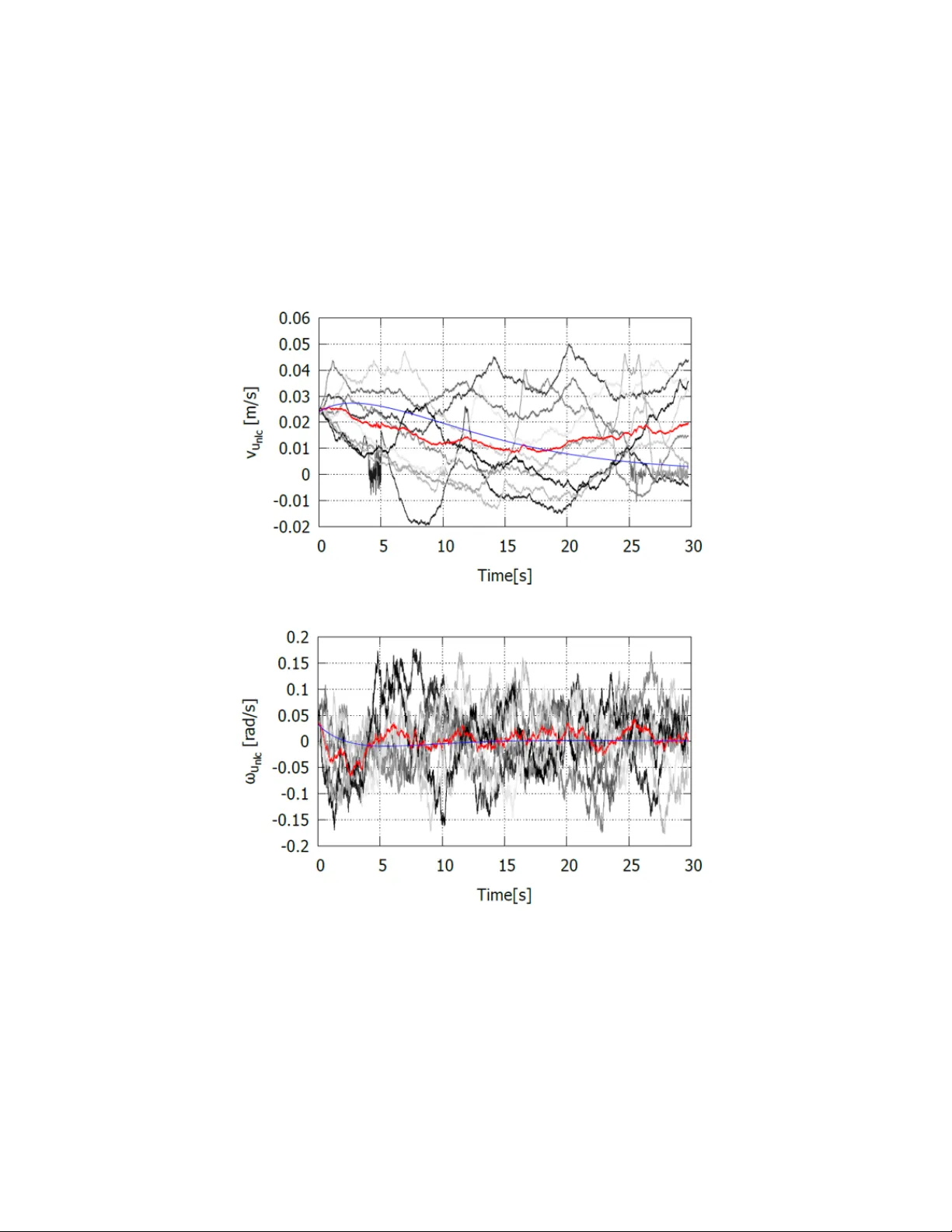
Sto c hastic Safet y-critical Con trol Comp ensating Safet y Probabilit y for Marine V essel T rac king T o o Matsuo ∗ , Y ˆ uki Nishimura † , Kenta Hoshino ‡ and Daisuke T abuc hi ∗ Marc h 30, 2026 ‡ Abstract A marine v essel is a nonlinear system sub ject to irregular disturbances suc h as wind and wa ves, whic h cause trac king errors betw een the nomi- nal and actual tra jectories. In this study , a nonlinear vessel maneuv ering mo del that includes a tracking con troller is formulated and then con- trolled using a linear approximation around the nominal tra jectory . The resulting sto c hastic linearized system is analyzed using a sto c hastic ze- roing con trol barrier function (ZCBF). A sto chastic safety comp ensator is designed to ensure probabilistic safety , and its effectiveness is verified through numerical sim ulations. 1 In tro duction Autonomous marine vessel control is an essential control application problem aimed at reducing lab or shortages and maritime accidents. Since vessel dynam- ics constitutes nonlinear control systems sub ject to disturbances such as wind and w av es, their con trol problems are generally c hallenging, and v arious meth- o ds ha ve b een dev elop ed. The basic mo delings of the system and control design pro cedures for the v essels are summarized in F ossen [3]. Recen tly , con trol designs that stabilize vessels to follo w a nominal tra jectory are prop osed based on nonlinear con trol theory [4, 12]. F ujii et al. [4] proposed a control design that stabilizes the vessel to track the nominal tra jectory based on input-to-state stability , and Saback et al. [12] dev elop ed a control approach based on nonlinear model predictive control. These strategies ac hieve compen- sation for obstacle av oidance, modeling errors, and disturbance suppression, whic h are essen tial from practical p ersp ectiv es. F or more flexible achiev ement of safety and ease of control design, control designs based on safet y-critical con trol theory are effective; see, for example ∗ Kagoshima Univ ersity † Ok a yama Univ ersity ‡ DENSO IT Laboratory § This work has b een submitted to the Journal of Marine Science and T ec hnology for possible publication. Copyrigh t ma y be transferred without notice, after whic h this version may no longer b e accessible. 1 Ames et al. [1]. Otsuki et al. [10] applies the safety-critical control theory into the tracking problem of a vessel by combining mo del predictive con trol with safet y-critical control for guidance in p ort en vironments. A t the same time, b ecause marine vessels are systems sub ject to v arious irregular disturbances, safety under disturbances is required to compensate as in [2]. When irregular disturbances are regarded as sto c hastic fluctuations, the systems are sometimes considered as sto c hastic systems [5, 6]. Maki et al. [5] analyzes the stabilizability and destabilizabilit y effects of the multiplicativ e sto c hastic fluctuations for ship’s maneuv ering motion. Maki et al. [6] analyzes the mechanism of parametric rolling in irregular seas based on sto c hastic Ly a- puno v stability theory . Ho wev er, to the best of the author’s kno wledge, the application of the recent results of sto chastic safet y-critical control theory to ship automation remains a c hallenging task. Safet y-critical control theory for stochastic systems are developed b y Pra- jana et al. [11], Xue et al. [13] and Nejati et al. [7] based on the sto c hastic safet y verification. These metho ds are effectiv e for complex safety-critical con- trol problems, while the analyzing and control metho ds are complicated. An adv an tage of safet y-critical control is its simple control design framew ork based on a control barrier function. T aking adv an tage of this feature, a stochastic safet y-critical control theory is prop osed b y Nishim ura and Hoshino [9]. F ur- thermore, an analytical method for safet y probability comp ensation in stable linear systems is developed b y Nishim ura and Hoshino [8]. In the metho ds, the diffusion coefficient, whic h directly c haracterizes the influence of disturbances on the system, explicitly app ears in the sufficient condition for safety . Therefore, in a con trol design that utilizes the sufficien t condition, the diffusion coefficient directly influences the con trol law. A t the same time, for the purp ose of com- p ensating for the influence of sto chastic noises of tracking problems, the results in [9] and [8] should be impro ved a little. In this pap er, we sligh tly mo dify the sto chastic safet y-critical control theory in [9] and [8], follo wed b y formulating a v essel maneuv ering mo del as a stochastic linear system sub ject to disturbances. Then, we apply the modified sto c hastic safet y-critical control technique to a trac king problem of a v essel under irregular disturbances so that the vessel remains within a designed region with a sp ecified probabilit y . The v alidit y of the designed compensator is confirmed b y n umerical sim ulation. This pap er is organized as follows. In Section 2 , we describ e our target system based on F ossen [3]. In Section 3, w e design a trac king controller us- ing the linear quadratic (LQ) control sc heme for the linearized system mo del. In Section 4, we analyze the safety probability , whic h is the probability that the error tra jectory remains the designed region when Gaussian white noise is in tro duced in to the linearized system. Then, in Section 5, w e design a linear comp ensator to increase the safet y probability for the linearized system, and in Section 6, we also design a nonlinear comp ensator of the safety probabilit y for the target nonlinear system. In Section 7, we confirm the v alidit y of the de- signed comp ensators b y numerical sim ulations. The safety-probabilit y control theory is prop osed in Section 8 by mo difying the results of [9] and [8], and in 2 Figure 1: marine vessel maneuvering kinematic mo del [3]. Figure 2: Marine vessel maneuvering kinematic mo del for nominal and actual tra jectories. Section 9, we conclude the pap er. 2 System Mo del In this section, we consider a marine v essel maneuvering kinematic mo del based on global p osition co ordinates based on [3]. Let the v ariables b e defined as sho wn in Fig. 1. Then w e obtain    ˙ x g lo = v sur cos θ g lo − v swa sin θ g lo , ˙ y g lo = v sur sin θ g lo + v swa cos θ g lo , ˙ θ g lo = ω y aw , (1) where x g lo [m] is the horizontal p osition of the marine vessel, y g lo [m] is vertical p osition of the marine vessel, θ g lo [rad] is the angle from the x g lo -axis, v sur [m/s] is surge velocity of the marine v essel, v swa [m/s] is swa y velocity , and ω y aw [rad/s] is ya w angular v elo cit y . In the same w ay as in [3], we mo dify the ab ov e mo del by pivoting on the p oin t, which serv es as the turning axis of the v essel. If the pivoting p oin t is 3 lo cated at a distance c [m] ahead of the vessel’s center of gravit y , w e hav e c = − v swa ω y aw , (2) where w e assume c  = − 1. By substituting (2) to (1), w e obtain a state-space mo del    ˙ x g lo = v sur cos θ g lo + cω y aw sin θ g lo , ˙ y g lo = v sur sin θ g lo − cω y aw cos θ g lo , ˙ θ g lo = ω y wa . (3) Here, defining the reference states x r , y r , and θ r and the reference control inputs v r and ω r with v r  = 0, the reference mo del for (3) is describ ed as follo ws:    ˙ x r = v r cos θ r + cω r sin θ r , ˙ y r = v r sin θ r − cω r cos θ r , ˙ θ r = ω r . (4) W e define th e trac king errors with respect to the reference states b y x e , y e , θ e . F rom the geometric relations illustrated in Fig. 2, these errors are given by    x e = ( x r − x g lo ) cos θ g lo + ( y r − y g lo ) sin θ g lo , y e = − ( x r − x g lo ) sin θ g lo + ( y r − y g lo ) cos θ g lo , θ e = θ r − θ g lo . (5) Differen tiating b oth terms of the abov e, the error dynamics is deriv ed as    ˙ x e = v r cos θ e + cω r sin θ e − v sur + y e ω y aw , ˙ y e = v r sin θ e − cω r cos θ e + ( c − x e ) ω y aw , ˙ θ e = ω r − ω y aw . (6) Moreo ver, we set new control inputs v and ω and design v sur = v r cos( θ e ) + v , (7) ω y aw = ω r cos( θ e ) + ω , (8) so that the righ t-hand sides of (6) become all zero as x e = y e = θ e = 0. Then, w e obtain ˙ x ( t ) = f ( x ( t )) + g ( x ( t )) u ( t ) , (9) where x = ( x e , y e , θ e ) T is a state v ector, u = ( v, ω ) T is a control input vector, and f ( x ) =   cω r sin θ e + ω r y e cos θ e v r sin θ e − ω r x e cos θ e ω r (1 − cos θ e )   , (10) g ( x ) =   − 1 y e 0 c − x e 0 − 1   . (11) 4 Finally , assuming that Gaussian white noise (roughly , dw ( t ) /dt , where w is a one-dimensional standard Wiener pro cess) is imp osed on the ab ov e mo del, we obtain the following stochastic system: dx ( t ) = { f ( x ( t )) + g ( x ( t )) u ( t ) } dt + Gdw ( t ) , (12) where G =   σ x σ y σ θ   (13) with σ x , σ y , σ θ b eing constants. Moreov er, we assume that g ( x ) T G  = 0 is satis- fied regardless of the v alue of x . Remark 1 The r e ason for employing the sto chastic differ ential e quation (12) is that the Wiener pr o c ess w ( t ) is the or etic al ly not differ entiable almost everywher e, while the Gaussian white noise is formal ly derive d as dw /dt . 3 Con trol Design for T ra jectory T racking In this section, w e design a tra jectory trac king con trol la w under the assumption of no noise. Because the target system (9) is a nonlinear system, assuming that the initial state x (0) is not so large, we consider the following linearized model: ˙ x ( t ) = Ax ( t ) + B u ( t ) , (14) where A = ∂ f ∂ x    x =0 =   0 ω r cw r − ω r 0 v r 0 0 0   , B = g (0) =   − 1 0 0 c 0 − 1   . (15) Since w e assume c  = − 1 and v r  = 0, ( A, B ) is controllable. Here, w e design the state-feedback la w u ( t ) = u tra ( x ( t )) so that the tra jec- tory trac king is ac hieved. Considering a linear state-feedbac k la w u tra ( x ) = − K x, (16) where K is a 2 × 3 matrix, if there exist 3 × 3 positive definite symmetric matrices P and Q satisfying the Lyapuno v equation P ¯ A + ¯ A T P = − Q (17) with ¯ A = A − B K , then x = 0 of the system (14) with (16) is asymptotically stable. T o determine the feedback gain K , w e design u tra ( x ) as a linear-quadratic (LQ) con trol la w; that is, K = − R − 1 B T P x, (18) 5 whic h minimizes the follo wing cost J ( x, u ) = Z ∞ 0 ( x T Q ′ x + u T Ru ) dt. (19) The matrix P is the p ositiv e definite solution of the following algebraic Riccati equation: P A + A T P − P B R − 1 B T P + Q ′ = 0 , (20) whic h results in (17) with (18) and Q = Q ′ + P B R − 1 B T P . 4 Safet y Probabilit y Analysis In this section, we consider the situation of the existence of noise for the lin- earized mo del (14), and derive the safety probability that remains within a safe set against the noise. Consider the linearized system with a linear state-feedbac k la w and Gaussian white noise; that is, (14) with u = u tra ( x ) and adding the diffusion term with G in (13), then w e obtain dx ( t ) = ¯ Ax ( t ) dt + Gdw ( t ) . (21) When there is no noise, trac king is achiev ed through the LQ control. How- ev er, when noise is in tro duced in to the system, the trac king error x may become large. Therefore, we design the acceptable error range and analyze the proba- bilit y that x remains within this range. A simple w ay to determine the range is to consider a sublev el set of the Lyapuno v function V ( x ) = x T P x ; that is, { x | V ( x ) ≤ M } for some M > 0, b ecause it is an inv arian t set when there is no noise for any M . Therefore, w e define h ( x ) = − x T P x + M (22) and χ = { x | h ( x ) > 0 } = { x | V ( x ) < M } , (23) where the function h ( x ) is said to b e a sto c hastic zeroing con trol barrier function (sto c hastic ZCBF) and χ is said to b e a safe set. The reason for defining χ as an op en set and using h ( x ) is to consider stochastic safety-critical control theory , whic h is proposed in Section 8 b elo w. Then, consider Theorem 2 (in Section 8). Let µ ∈ (0 , M ) and b = eigmin[ Q ] − eigmin[ P ] tr[ G T P G ] M − µ 2eigmax[ P GG T P ] , (24) 6 Figure 3: The brief sketc h of the Lyapuno v function V ( x ), the sto c hastic ZCBF h ( x ), the safe set χ and the initial state set χ h>µ for a state space ( x 1 , x 2 ) T . where tr[ X ] is the trace, eigmax[ X ] is the maxim um eigen v alue, and eigmin[ X ] is the minim um eigenv alue of a p ositiv e semi-definite matrix X , respectively . If b > 0; that is, M − µ > tr[ G T P G ] eigmin[ P ] eigmin[ Q ] (25) is satisfied for some µ ∈ (0 , M ), the system (21) is safe in ( χ h>µ , χ, 1 − e − bµ ), whic h means that, if the initial v alue x (0) is in the initial state set χ h>µ = { x | h ( x ) > µ } = { x | V ( x ) ≤ M − µ } , the state x ( t ) remains the safe set χ for all t ≥ 0 at least the probability of 1 − e − bµ . The specific image for the relationship betw een the Ly apunov function V ( x ), the sto chastic ZCBF h ( x ), the safe set χ and the initial state set χ h>µ is drawn in Fig. 3, provided that the state space is reduced to t wo dimensions ( x 1 , x 2 ) T to simplify drawings. 5 Sto c hastic Safet y-critical Comp ensation b y Lin- ear State F eedbac k In this section, w e design a linear comp ensator u com ( x ( t )) = − K ′ x for the stabilized system (21) to increase the probabilit y that the error state vector x k eeps sta ying at χ . T o do this, we consider the system (14) with u = u tra ( x ) + u com ( x ) and (16) under the additiv e noise; that is, dx ( t ) = ( ¯ Ax ( t ) + B u com ( x ( t ))) dt + Gdw ( t ) . (26) W e also consider the sto c hastic ZCBF h ( x ) in (22) and the safe set χ in (23). 7 Set u com ( x ) = − R ′− 1 B T P x, (27) where R ′ is a 2 × 2 p ositiv e definite and symmetric matrix. Then, according to Corollary 1 (in Section 8), w e ac hieve that the system (14) with u = u tra ( x ) + u com ( x ) = − ( R − 1 + R ′− 1 ) B T P x is safe in ( χ h>µ , χ, 1 − e − ( b + b ′ ) µ ) with b + = G T B R ′ B T G G T G . (28) Because we assume B T G  = 0, b + > 0 is satisfied. Thus, the addition of u com ( x ) increases the safety probabilit y; that is, 1 − e − ( b + b ′ ) µ > 1 − e − bµ . 6 Sto c hastic Safet y-critical Comp ensation b y Non- linear State F eedbac k In this section, w e consider the nonlinear system (12) with u ( t ) = u tra ( x ) + u nlc ( x ), where u nlc ( x ) is a nonlinear compensator. If the initial v alue of the state x (0) is not so large, the b ehavior of the system (12) is approximated by the linearized system (14). If the noise is not v ery large, the linear compensator u com ( x ) ac hieves high safety probabilit y as stated in the previous section. Ho wev er, b ecause we consider Gaussian white noise, the impact of noise could b ecome extremely large instantaneously , and in suc h cases, the state v alue ma y also b ecome large. Therefore, in this section, w e design a nonlinear comp ensator for the nonlinear system (12). Letting a design parameter b ′ > 0 and γ ( x, b ) = 2 x T P ( f ( x ) + g ( x ) u tra ( x ) + b ′ GG T P x ) + G T P G, (29) w e design ϕ s ( x ) as follows: if γ ( x, b ) > 0 and x T P g ( x )  = 0, ϕ s ( x ) = − u tra ( x ) − 2 x T P ( f ( x ) + b ′ GG T P x ) + G T P G 2 x T P g ( x ) g T ( x ) P x g T ( x ) P x ; (30) otherwise, ϕ s ( x ) = 0. Moreo ver, we consider u nlc ( x ) :=    ϕ s ( x ) , h ( x ) ≤ µ ϕ ′ s ( x ) , h ( x ) ∈ ( µ, M ′ ) 0 , h ( x ) ≥ M ′ (31) and ϕ ′ s ( x ) = ϕ s ( x ) h ( x ) − M ′ µ − M ′ , (32) 8 where M ′ ∈ ( µ, M ] is designed so that u nlc = 0 for all x ∈ χ h>M ′ ⊂ χ h>µ . Using Corollary 2, w e see that the system (12) with control input u = u nlc ( x ) is safe in ( χ h>µ , χ, 1 − e − b ′ µ ). Moreo ver, if 2 x T P ( f ( x ) + b ′ GG T P x ) + G T P G > 0 (33) holds for all x ∈ χ µ with some µ > 0 satisfying x T P g ( x ) = 0, u nlc ( x ) is con tinuous regardless of the v alue of x . 7 Numerical Sim ulation 7.1 P arameter Settings In this section, w e confirm the v alidity of the safet y-probability comp ensators b y calculating concrete problem settings and their numerical sim ulation. W e first consider to add the LQ controller u tra ( x ) with (16) without any safet y-probability comp ensator; that is, u = u tra ( x ). Setting c = 3, ω r = 0 . 1, and v r = 1, w e obtain A =   0 0 . 1 0 . 3 − 0 . 1 0 1 0 0 0   , B =   − 1 0 0 3 0 − 1   , (34) and b y setting Q ′ =   0 . 1 0 0 0 0 . 3 0 0 0 0 . 2   , R =  40 0 0 40  , (35) the matrix P is obtained as P =   1 . 99 − 0 . 06 − 0 . 92 − 0 . 06 2 . 64 11 . 32 − 0 . 92 11 . 32 63 . 81   . (36) Th us, the feedbac k gain K is obtained as K =  − 0 . 05 0 . 00 0 . 02 0 . 02 − 0 . 09 − 0 . 75  (37) and the ¯ A = A − B K is giv en b y ¯ A =   − 0 . 05 0 . 10 0 . 32 − 0 . 16 0 . 25 3 . 24 0 . 02 − 0 . 08 − 0 . 75   . (38) Moreo ver, the diffusion co efficien t G is assumed to be G =   0 . 08 0 . 08 0 . 08   . (39) 9 T o satisfy the condition (25), M − µ > 3 . 53 is needed. Noting the condition, w e set M = 10 and µ = 1; then, we obtain b = 0 . 0043, and the system (14) with u = u tra ( x ) is safe in ( χ h>µ , χ, 0 . 0043). Next, to enhance the safet y of the safe set, w e consider to design the linear safet y-probability comp ensator u com ( x ) giv en b y (27). By c ho osing R ′ =  15 0 0 15  , (40) w e obtain b + = 5 . 79 from (28). Thus, the system (14) with u = u tra ( x )+ u com ( x ) is safe in ( χ h>µ , χ, 0 . 997). Finally , w e emplo y the nonlinear safet y-probability comp ensator u nlc ( x ) giv en by (31) and apply u = u tra ( x ) + u nlc ( x ) to the system (12). Setting b ′ = 3 and M ′ = 9, the system is safe in ( χ h>µ , χ, 0 . 950). 7.2 Sim ulation Results In this subsection, we compare the safety-probabilit y performances of the three con trollers u = u tra ( x ), u = u tra ( x ) + u com ( x ) and u = u tra ( x ) + u nlc ( x ) for the target nonlinear sto chastic system (12) through numerical sim ulations. F or all simulations, we set the initial state vector x (0) = (0 . 5 , 0 . 5 , 0) T , and th us h ( x 0 ) = 8 . 87. F or each condition, w e p erform ten simulations with G in (39) and one simulation with G = 0. Figs. 4–13 show the results of u = u tra ( x ), u = u tra ( x ) + u com ( x ) and u = u tra ( x ) + u nlc ( x ), respectively . The ten sample paths are depicted b y gra y lines, the a verage of the sample paths is shown b y the red line, and the results without noise (that is, G = 0) are shown by the blue line. Moreo ver, the purple lines in Figs. 4, 5, 6, 7, 10, and 11 indicate the b oundary of the safe set χ , and the green line in Figs. 5, 7, 11 indicates the b oundary of the initial state set χ h>µ . When u = u tra ( x ); that is, without any safet y-probability compensator, h ( x ) tak es negativ e v alues as shown in Fig. 5; therefore, in Fig. 4, the tra jectories of x escap e from the b oundary of the safe set. This result accurately reflects the theoretically calculated safety probabilit y of 0 . 0043. When u = u tra ( x ) + u com ( x ); that is, with the linear safety-probabilit y comp ensator, all sample paths remain in the safe set h ( x ) > 0 as shown in Fig. 7; therefore, in Fig. 6,the tra jectories of x also remain inside the safe set. This result accurately reflects the theoretically calculated safet y probabilit y of 0 . 997. When u = u tra ( x ) + u nlc ( x ); that is, with the nonlinear safety-probabilit y comp ensator, all sample paths remain in the safe set h ( x ) > 0 as shown in Fig. 11; therefore, in Fig. 10, the tra jectories of x also remain inside the safe set. This result accurately reflects the theoretically calculated safet y probabilit y of 0 . 950. 10 8 Theory 8.1 Notations Let R n b e an n -dimensional Euclidean space and esp ecially , R := R 1 . A Lie deriv ative of a smo oth mapping W : R n → R in a mapping F = ( F 1 , ..., F q ) : R n → R n × R q with F 1 , ..., F q : R n → R n is denoted by L f W ( x ) =  ∂ W ∂ x F 1 ( x ) , ..., ∂ W ∂ x F q ( x )  . (41) F or constants a, b > 0, a contin uous mapping α : [ − b, a ] → R is said to b e an extended class K function if it is strictly increasing and satisfies α (0) = 0. A class K function α is said to b e of class K ∞ if lim s →∞ α ( s ) = ∞ . If a function α is r times contin uously differentiable, it is denoted as C r . The boundary of a set A is denoted b y ∂ A . Let (Ω , F , {F t } t ≥ 0 , P ) be a filtered probability space where Ω is the sample space, F is the σ -algebra that is a collection of all the even ts, {F t } t ≥ 0 is a filtration of F and P is a probabilistic measure. In the filtered probabilit y space, P [ A | A o ] denotes the probability of some even t A under some condition A o and W t is a d -dimensional standard Wiener process. F or a Marko v pro cess X t ∈ R n with an initial state X t = x 0 , we often use the following notation P x 0 [ A ] = P [ A | X 0 = x 0 ]. The differen tial form of an Itˆ o in tegral of f : R n → R n o ver W t is represen ted b y f ( x ) dW t . The trace of a square matrix Q is denoted b y tr[ Q ]. 8.2 Sto c hastic System W e consider the following stochastic system: dX t = { f ( X t ) + g ( X t )( u o ( X t ) + u ( t )) } dt + σ ( X t ) dW t , (42) where X t ∈ R n is a state vector with a fixed initial v alue x 0 = x (0) ∈ R n , u o : R n → R m is a pre-input assumed to b e a contin uous state-feedback, u ∈ U ⊂ R m is a compensator for safet y-critical control, where U denotes an admissible con trol set, and maps f : R n → R n , g : R n → R n × R m , σ : R n → R n × R d are assumed to b e all locally Lipschitz. The lo cal Lipschitz condition on f , g , σ implies the existence of a stopping time T > 0 suc h that ( X t ) t 0, for an y sup erlevel set { x ∈ R n | h ( x ) ≥ L } is compact. ( Z3 ) The closure of χ is the 0-superlevel set of h ( x ); that is, χ = { x ∈ R n | h ( x ) > 0 } , (47) ∂ χ = { x ∈ R n | h ( x ) = 0 } (48) are both satisfied. W e set some sets and stopping times used in this subsection. F or µ > 0, let χ µ := { x ∈ R n | h ( x ) ∈ (0 , µ ] } ⊂ χ (49) χ h>µ := χ \ χ µ = { x ∈ R n | h ( x ) > µ } (50) R n h ≤ µ := ˜ χ ∪ χ µ = { x ∈ R n | h ( x ) ≤ µ } (51) b e defined. F or a solution to system (42) with x 0 ∈ χ , the first exit time from χ is denoted by τ 0 . Let p ∈ [0 , 1]. System (42) said to b e safe in ( χ h>µ , χ, p ) if, for an y x 0 ∈ χ h>µ , P x 0  inf t ≥ 0 h ( X t ∧ τ 0 ) > 0  ≥ p (52) is satisfied. T o analyze the safety of a sto c hastic system, w e define the follo wing: Definition 1 (Sto chastic ZCBF [8]) L et (42) b e c onsider e d with χ and h ( x ) satisfying (Z1), (Z2) and (Z3). If ther e exist c ontinuous mapping ϕ : R n → R m and b > 0 such that, for al l x ∈ R n h ≤ µ , L f ,g,σ ( u o ( x ) , ϕ ( x ) , h ( x )) ≥ bH σ ( h ( x )) (53) is satisfie d with some b > 0 , then h ( x ) is said to b e a stochastic zeroing con trol barrier function (ZCBF) . Theorem 1 L et the system (42) b e c onsider e d. If ther e exists a sto chastic ZCBF h ( x ) , then the system b e c omes safe in ( χ h>µ , χ, 1 − e − bµ ) by designing u = ϕ ( x ) that satisfies al l the c onditions in Definition 1. ♦ 12 The proof for Theorem 1 is written in App endix A b elow. Remark 2 The r esults of this subse ction ar e differ ent fr om those in [9] in two p oints. The first is that we define safe in ( χ h>µ , χ, p ) , which is the notion for a glob al time; in c ontr ast, the pr evious work c onsiders tr ansiently safe, which is the notion for a sp e cific Markov time. The other is that we set the initial state set (the first element of the triple for safety) as χ h>µ , while the pr evious work c onsiders the initial state set as χ µ . The change in the initial state enables us to c onsider safety in glob al time. ♢ 8.3.2 Safety Probabilit y Analysis and Linear Con trol Design F or Sto c hastic Linear Systems In this subsection, w e improv e the design comp ensators of the safet y probability for a linear system with additive noises by improving the results of [8] using the safet y prop osed in the previous subsection. Consider a linear system with additiv e noise dX t = ( AX t + B u o ( X t )) dt + GdW t , (54) whic h is (42) with f ( x ) = Ax , g ( x ) = B , σ ( x ) = G and u = 0, where A ∈ R n × n , B ∈ R n × m and G ∈ R n × d . Theorem 2 L etting u o ( x ) = − B K x with K ∈ R m × n and ¯ A = A − B K , assume that ther e exist p ositive definite and symmetric matric es P, Q ∈ R n × n satisfying a Lyapunov e quation P ¯ A + ¯ A T P = − Q. (55) L et us also c onsider a c andidate for a sto chastic ZBF h ( x ) = − x T P x + M , M > 0 , (56) a safe set χ and the r elate d sets χ µ , χ h>µ , and R n h ≤ µ with µ ∈ (0 , M ) . If L := eigmin[ Q ] − eigmin[ P ] tr[ G T P G ] M − µ > 0 (57) is satisfie d, then the system (54) is safe in ( χ h>µ , χ, 1 − e − bµ ) , wher e b ≤ L 2eigmax[ P GG T P ] . (58) ♦ The proof for Theorem 2 is written in App endix B b elow. Next, w e consider adding the comp ensator u for (54); that is, dX t = ( AX t + B ( u o ( X t ) + u ( t ))) dt + GdW t . (59) 13 Corollary 1 Assume that the c onditions in The or em 2 ar e al l satisfie d. If ther e exist a p ositive definite and symmetric matrix R ∈ R m × R m and b + > 0 such that B R − 1 B T = b + GG T , (60) then, the system (59) with u = ϕ po ( x ) , wher e ϕ po ( x ) := − R − 1 B T P x, (61) is safe in ( χ h>µ , χ, 1 − e − ( b + b + ) µ ) . ♦ The proof for Corollary 1 is sho wn in Appendix C. 8.3.3 Safety Probabilit y Con trol Design F or Sto c hastic Nonlinear Systems In this subsection, we provide the design pro cedure for a comp ensator of the safet y probability for a nonlinear system by applying our result of Theorem 1 to the result of [9]. Corollary 2 L et the system (42) b e c onsider e d with the safe set χ and a c an- didate of a sto chastic ZCBF h ( x ) satisfying al l the c onditions of (Z1)–(Z3). L et I s ( u o ( x ) , h ( x )) := L f ,g,σ (0 , u o ( x ) , h ( x )) (62) J s ( h ( x )) := bH σ ( h ( x )) (63) and ϕ s : R n → R m b e designe d as ϕ s ( x ) = − I s ( u o ( x ) , h ( x )) − J s ( h ( x )) L g h ( x )( L g h ( x )) T ( L g h ( x )) T (64) for I s < J s ∩ L g h  = 0 , and ϕ s ( x ) = 0 for I s ≥ J s ∪ L g h = 0 . Mor e over, we c onsider Φ s :=  ϕ s , x ∈ R n h ≤ µ , ϕ ′ s , x ∈ χ h>µ , (65) wher e ϕ ′ s : χ h>µ → R m is c ontinuous and satisfies ϕ ′ s ( x ) = ϕ s ( x ) for al l x ∈ ∂ χ h>µ . If, for al l x ∈ χ µ with some µ > 0 satisfying L g h = 0 , L f h ( x ) + L I σ ( h ( X )) > bH σ ( h ( x )) (66) holds, then Φ s is c ontinuous al l in R n and the system (42) with u = Φ s ( x ) is safe in ( χ h>µ , χ, 1 − e − bµ ) . ♦ While the pro of is quite similar to Corollary 2 in [9], w e describ e it App endix D for the sake of self-containmen t in this pap er. 14 9 Conclusion In this pap er, w e mo dified sto c hastic safety-critical con trol theory using the sto c hastic zeroing con trol barrier function (ZCBF) in [8] and applied it to safety- critical compensation for a tra jectory tracking problem of marine vessels sub ject to irregular disturbances. The error dynamics of the v essel motion is stated in the state-space mo del and the tracking control is ac hieved by linear quadratic con trol for the linearized mo del. The safet y probability was defined as the prob- abilit y that the error tra jectory remains the designed region against irregular disturbances, which is assumed to b e Gaussian white noise. Then, the linear and nonlinear safet y probabilit y compensators w ere proposed based on the mod- ified stochastic safety-critical control theory , and the effects of the compensators w ere confirmed b y n umerical sim ulation. References [1] A. D. Ames, S. Co ogan, M. Egerstedt, G. Notomista, K. Sreenath, and P . T abuada. Con trol barrier functions: theory and applications. Pr o c. 18th Eur o. Contr ol Conf. , pages 3420–3431, 2019. [2] H. N. Esfahani and R. Szlap czynski. Robust-adaptiv e dynamic programming-based time-dela y control of autonomous ships under sto c has- tic disturbances using an actor-critic learning algorithm. J Marine Sci T e chnol , 26(4):1262–1279, 2021. [3] T. I. F ossen. Handb o ok of Marine Cr aft Hydr o dynamics and Motion Con- tr ol . John Wiley & Sons Ltd., Chic hester, UK, second edition, 2021. [4] Y. F ujii, H. Nak amura, and Y. Sato. Stability gain design metho d based on L 2 norms for differen tially flat systems. T r ansactions of the So ciety of Instrument and Contr ol Engine ers , 56(5):259–268, 2020. [5] A. Maki, K. Hoshino, L. Dostal, Y. Maruy ama, F. Hane, and Y. Y oshimura. Sto c hastic stabilization and destabilization of ship maneuvering motion by m ultiplicative noise. J Marine Sci T e chnol , 28(8):704–718, 2023. [6] A. Maki, Y. Maruyama, Y. Liu, and L. Dostal. Comparison of sto c hastic stabilit y b oundaries for parametrically forced systems with application to ship rolling motion. J Marine Sci T e chnol , 29(5):446–456, 2024. [7] A. Nejati, S. Soudjani, and M. Zamani. Comp ositional construction of con- trol barrier functions for contin uous-time sto c hastic h ybrid systems. A uto- matic a , 145:110513, 2022. [8] Y. Nishim ura and K. Hoshino. Safet y-probability analysis and control for sto c hastic systems based on lyapuno v candidate functions. Pr o c. 62nd IEEE Conf. De cis. Contr. , pages 4818–4823, 2023. 15 [9] Y. Nishim ura and K. Hoshino. Control barrier functions for sto c hastic systems and safety-critical con trol designs. IEEE T r ans. Autom. Contr ol , 69(11):8088–8095, 2024. [10] S. Otsuki, N. Hatta, M. Hanif, T. Hatanak a, and K. Nak ashima. Hierarchi- cal v essel autonomous op eration in a p ort with safet y certificates: com bined mp c and cbf approach. Pr o c. IF A C World Congr ess 2023 , pages 3481–3488, 2023. [11] S. Pra jna, A. Jadbabaie, and G. J. Pappas. A framework for worst-case and sto c hastic safet y v erification using barrier certificates. IEEE T r ans. A utom. Contr ol , 52(8):1415–1428, 2007. [12] R. M. Saback, A. G. S. Conceicao, T. L. M. Santos, J. Albiez, and M. Reis. Nonlinear mo del predictive control applied to an autonomous underwater v ehicle. IEEE J. Oc e anic Engine ering , 45(3):799–812, 2020. [13] B. Xue, N. Zhan, and M. F ranzle. Reach-a void analysis for stochastic differen tial equations. IEEE T r ans. Autom. Contr ol , 69(3):1882–1889, 2024. A Pro of of Theorem 1 A.1 Existence of Solution First, we pro ve that the existence of a sto c hastic ZCBF h ( x ) ensures that the system (42) with u = ϕ ( x ) has a solution in global time. T o do this, we consider the follo wing definition and theorem. Definition 2 (FCiP , [8]) L et system (42) b e c onsider e d with u = ϕ ( x ) , wher e ϕ : R n → R m is a c ontinuous mapping. If a C 2 mapping Y : R n → [0 , ∞ ) is pr op er; that is, for any L ∈ [0 , ∞ ) , any sublevel set { x ∈ R n | Y ( x ) ≤ L } is c omp act, and a c ontinuous mapping ψ : [0 , ∞ ) × (0 , 1) → [0 , ∞ ) b oth exist for every x 0 ∈ R n such that P x 0 [ ∀ t ∈ [0 , l ] , Y ( X t ) ≤ ψ ( l, ϵ )] ≥ 1 − ϵ (67) holds for al l l ∈ [0 , ∞ ) and al l ϵ ∈ (0 , 1] , then the system is said to b e forwar d c omplete in pr ob ability (FCiP). ■ Theorem 3 ([8]) L et us c onsider system (42) , a c ontinuous mapping ϕ : R n → R m and an initial c ondition x 0 ∈ R n . If ther e exists a pr op er and C 2 mapping Y : R n → [0 , ∞ ) such that L f ,g,σ ( ϕ ( x ) , u o ( x ) , Y ( x )) ≤ c 1 Y ( x ) + c 2 (68) is satisfie d for al l x ∈ R n and for some c 1 ∈ [0 , ∞ ) and c 2 ∈ [0 , ∞ ) , then the system with u = ϕ ( x ) is FCiP. ♦ 16 Let h b ( x ) := e bh ( x ) . (69) Because L D f ,g ( ϕ ( x ) , u o ( x ) , h b ( x )) = bh b ( x ) L D f ,g ( ϕ, u o ( x ) , h ( x )) , (70) is satisfied, (53) changes as follo ws: L D f ,g ( ϕ ( x ) , u o ( x ) , h b ( x )) ≥ bh b ( x )  bH σ ( h ( x )) − L I σ ( h ( x ))  . (71) Moreo ver, letting B b ( x ) := ( h b ( x )) − 1 = e − bh ( x ) , (72) w e obtain L I σ ( B b ( x )) = bB b ( x )  bH σ ( h ( x )) − L I σ ( h ( x ))  , (73) whic h transforms (71) in to L D f ,g ( ϕ, u o ( x ) , h b ( x )) ≥ ( h b ( x )) 2 L I σ ( B b ( x )) . (74) Therefore, using the relationship L D f ,g ( u, u o ( x ) , h b ( x )) = − ( h b ( x )) 2 L D f ,g ( u, u o ( x ) , B b ( x )) , (75) w e obtain − L D f ,g ( ϕ, u o ( x ) , B b ( x )) ≥ L I σ ( B b ( x )); (76) that is, L f ,g,σ ( ϕ, u o ( x ) , B b ( x )) ≤ 0 , x ∈ R n h ≤ µ . (77) Here, we consider the rest space χ h>µ , where the assumption (Z2) implies that the space is bounded and h is b ounded from abov e in the space. In addition, B b is decreasing, u o is con tinuous, and f , g , and σ are all lo cally Lipsc hitz. Therefore, L f ,g,σ ( ϕ, u o ( x ) , B b ( x )) is bounded from abov e; that is, for sufficien tly large v alues c 1 > 0 and c 2 > 0, w e obtain L f ,g,σ ( ϕ, u o ( x ) , B b ( x )) ≤ c 1 B b ( x ) + c 2 , x ∈ χ h>µ . (78) Considering (77) and (78), all the conditions of Theorem 3 are satisfied with Y = B b ; that is, the system (42) with u = ϕ ( x ) is F CiP . 17 A.2 Safet y Probabilit y Next, considering { X t ∈ χ, ∀ t ≥ 0 } = { τ 0 = ∞} (79) = { inf t ≥ 0 h ( X t ) > 0 } (80) = { inf t ≥ 0 h ( X t ∧ τ 0 ) > 0 } (81) = { sup t ≥ 0 B b ( X t ∧ τ 0 ) < 1 } (82) and Mark ov inequality , for x ∈ χ h>µ , P x 0  { sup t ≥ 0 B b ( X t ∧ τ 0 ) ≥ m } ∩ { τ µ < ∞}  ≤ E x 0  sup t ≥ 0 B b ( X t ∧ τ 0 ) I { τ µ < ∞}  m (83) for an y m > 0. Cho osing m = 1, w e obtain P x 0  { inf t ≥ 0 h ( X t ∧ τ 0 ) ≤ 0 } ∩ { τ µ < ∞}  = P x 0  { sup t ≥ 0 B b ( X t ∧ τ 0 ) ≥ 1 } ∩ { τ µ < ∞}  (84) ≤ E x 0  sup t ≥ 0 B b ( X t ∧ τ 0 ) I { τ µ < ∞}  . (85) Here, considering the strong Mark ov prop ert y , w e obtain E x 0  sup t ≥ 0 B b ( X t ∧ τ 0 ) I { τ µ < ∞}  = E x 0 " E x τ µ " sup t ≥ τ µ B b ( X ( t − τ µ ) ∧ τ 0 ) # I { τ µ < ∞} # (86) ≤ E x 0  B b ( X τ µ ) I { τ µ < ∞}  (87) = e − bµ P x 0 [ { τ µ < ∞} ] , (88) where w e use Dynkin’s formula with the giv en condition (77): E x τ µ  B b ( X ( t − τ µ ) ∧ τ 0 )  − B b ( X τ µ ) (89) = E x τ µ " Z ( t − tµ ) ∧ τ 0 τ µ L f ,g,σ ( ϕ ( X τ ) , u o ( X τ ) , B b ( X τ ) dτ # ≤ 0 . (90) 18 Substituting the ab ov e result to (85), we obtain P x 0  { inf t ≥ 0 h ( X t ∧ τ 0 ) ≤ 0 } ∩ { τ µ < ∞}  ≤ e − bµ P x 0 [ { τ µ < ∞} ]; (91) th us, P x 0 [ { X t ∈ χ, ∀ t ≥ 0 } ∩ { τ µ < ∞} ] = P x 0  { inf t ≥ 0 h ( X t ∧ τ 0 ) > 0 } ∩ { τ µ < ∞}  (92) ≥ (1 − e − bµ ) P x 0 [ { τ µ < ∞} ] (93) On the other hand, for x ∈ χ h>µ , w e obtain P x 0 [ { X t ∈ χ, ∀ t ≥ 0 } ∩ { τ µ = ∞} ] = P x 0 [ { τ µ = ∞} ] (94) ≥ (1 − e − bµ ) P x 0 [ { τ µ = ∞} ] (95) Com bining (95) and (93), w e obtain P x 0 [ { X t ∈ χ, ∀ t ≥ 0 } ] = P x 0 [ { X t ∈ χ, ∀ t ≥ 0 } ∩ { τ µ = ∞} ] + P x 0 [ { X t ∈ χ, ∀ t ≥ 0 } ∩ { τ µ < ∞} ] (96) ≥ (1 − e − bµ ) ( P x 0 [ { τ µ = ∞} ] + P x 0 [ { τ µ < ∞} ]) (97) = 1 − e − bµ . (98) This completes the pro of. B Pro of of Theorem 2 This theorem is pro v en by sho wing that h ( x ) is a stochastic ZCBF. In the pro of, w e often use the relationship eigmin[ Y ] x T x ≤ x T Y x ≤ eigmax[ Y ] x T x (99) for a symmetric matrix Y ∈ R n × R n . First, because the assumption of (53) has to hold for x ∈ R n h ≤ µ ; that is, x T P x ≥ M − µ. (100) Therefore, it is sufficient for x T x ≥ M − µ eigmin[ P ] (101) 19 to satisfy assumption (53). On the other hand, the giv en assumptions (57) and (58) yield eigmin[ Q ] − 2 b · eigmax[ P GG T P ] ≥ eigmax[ P ] tr[ G T P G ] M − µ . (102) Th us, we obtain the follo wing condition of M − µ eigmin[ P ] ≥ tr[ G T P G ] eigmin[ Q ] − 2 b · eigmax[ P GG T P ] . (103) This results in x T x ≥ tr[ G T P G ] eigmin[ Q ] − 2 b · eigmax[ P GG T P ] . (104) Applying (99) to the ab o ve inequality , w e obtain x T Qx − tr[ G T P G ] ≥ 2 bx T P GG T P x, (105) whic h is the same as L Ax,B ,G (0 , − B K x, h ( x )) ≥ bH G ( h ( x )) . (106) This is a sufficient condition that h ( x ) is a sto c hastic ZCBF with ϕ = 0. Con- sequen tly , b y Theorem 1, the system is safe in ( χ h>µ , χ, 1 − e − bµ ). C Pro of of Corollary 1 Considering u = ϕ po ( x ) with (61) and h ( x ) with (56), we obtain L Ax,B ,G ( ϕ po ( x ) , − B K x, h ( x )) = x T Qx − tr  G T P G  + 2 x T P B R − 1 B T P x ; (107) th us, applying (106), w e obtain L Ax,B ,G ( ϕ po ( x ) , − B K x, h ( x )) ≥ 2 bx T P GG T P x + 2 x T P B R − 1 B T P x. (108) Moreo ver, w e also consider the additional assumption (60), the ab o ve inequalit y results in L Ax,B ,G ( ϕ po ( x ) , − B K x, h ( x )) ≥ 2( b + b + ) x T P GG T P x, (109) whic h implies (53), pro vided that b is replaced by b + b + . This completes the pro of. 20 D Pro of of Corollary 2 First, consider the case L g h  = 0 in χ µ . If I s < J s , w e obtain L f ,g,σ ( ϕ s ( x ) , u o ( x ) , h ( x )) = bH σ ( h ( x )) (110) and if I s ≥ J s , w e obtain L f ,g,σ ( ϕ s ( x ) , u o ( x ) , h ( x )) = I s ( u o ( x ) , h ( x )) ≥ J s ( h ( x )) = bH σ ( h ( x )) . Therefore, regardless of I s < J s or I s ≥ J s , the inequality (53) is satisfied. Moreo ver, because L g h ( x ), I s ( u o ( x ) , h ( x )) and J s ( h ( x )) are all contin uous in L g h ( x )  = 0 and ϕ s ( x ) → 0 as I s → J s uniformly when L g h ( x )  = 0, ϕ s ( x ) is con tinuous in L g h ( x )  = 0. Then, we consider the other case, i.e., L g h = 0 in χ µ . The additional condition (66) implies that there exists a sufficiently small constan t ϵ > 0 such that L f h ( x ) + L I σ ( h ( x )) − ϵ ≥ bH σ ( h ( x )) (111) is satisfied. Combining the inequality and the assumption of u o to be contin uous, for a subset G oµ ⊂ χ µ , whic h is a neighborho od of x g ∈ { x ∈ χ µ | L g h ( x ) = 0 } || L g h ( x ) u o ( x ) || ≤ ϵ (112) is satisfied. Thus, for x ∈ G oµ , w e obtain L f h ( x ) + L I σ ( h ( x )) + L g h ( x ) u o ( x ) ≥ bH σ ( h ( x )) , (113) whic h implies that I s ≥ J s ; namely , ϕ s = 0 in G o . Therefore, ϕ s is contin uous around L g h ( x ) = 0 in χ µ . Consequen tly , ϕ s is alwa ys con tinuous in χ and satisfies all the assumptions and conditions of Theorem 1. Moreov er, because u = ϕ ′ s ( x ) is contin uous in χ h>µ and ϕ ′ s ( x ) = ϕ s ( x ) for all x ∈ ∂ χ h>µ , u is contin uous for all χ . This completes the pro of. 21 Figure 4: T ra jectories with u = u tra and safet y boundary . Figure 5: Time resp onses of h ( x ) with u = u tra . 22 Figure 6: T ra jectories with u = u tra + u com and safet y boundary . Figure 7: Time resp onses of h ( x ) with u = u tra + u com . 23 Figure 8: Time resp onses of v com . Figure 9: Time resp onses of ω com . 24 Figure 10: T ra jectories with u = u tra + u nlc and safet y boundary . Figure 11: Time resp onses of h ( x ) with u = u tra + u nlc . 25 Figure 12: Time resp onses of v nlc . Figure 13: Time resp onses of ω nlc . 26