Stability and Sensitivity Analysis of Relative Temporal-Difference Learning: Extended Version

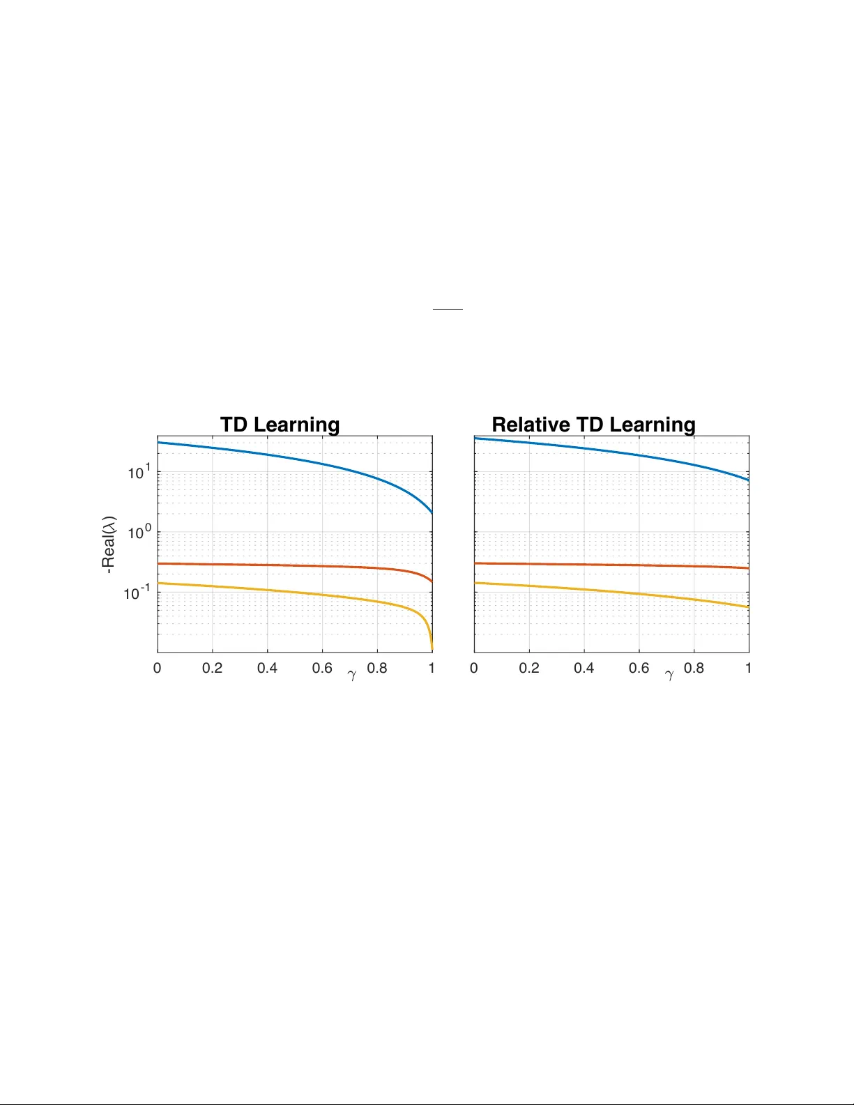
Stabilit y and Sensitivit y Analysis of Relativ e T emp oral-Difference Learning: Extended V ersion Masoud S. Sakha † , Rushik esh Kamalapurk ar † and Sean Meyn* Marc h 31, 2026 Abstract Relativ e temp oral-difference (TD) learning was introduced to mitigate the slo w con vergence of TD metho ds when the discount factor approac hes one by subtracting a baseline from the temp oral-difference update. While this idea has b een studied in the tabular setting, stabilit y guaran tees with function appro ximation remain p oorly understoo d. This pap er analyzes rela- tiv e TD learning with linear function appro ximation. W e establish stability conditions for the algorithm and sho w that the choice of baseline distribution plays a central role. In particular, when the baseline is c hosen as the empirical distribution of the state–action pro cess, the algo- rithm is stable for any non-negativ e baseline w eight and an y discount factor. W e also provide a sensitivity analysis of the resulting parameter estimates, characterizing b oth asymptotic bias and co v ariance. The asymptotic co v ariance and asymptotic bias are sho wn to remain uniformly b ounded as the discount factor approaches one. Keyw ords: reinforcemen t learning; optimal control. Con ten ts 1 In tro duction 2 2 Main Results 6 3 Sim ulations 9 3.1 Finite-state Finite-action MDP . . . . . . . . . . . . . . . . . . . . . . . . . . . . . . 9 3.2 Sp eed scaling . . . . . . . . . . . . . . . . . . . . . . . . . . . . . . . . . . . . . . . . 13 3.3 Discussion. . . . . . . . . . . . . . . . . . . . . . . . . . . . . . . . . . . . . . . . . . 14 4 Conclusions 14 A Appendices 17 A.1 Diric hlet forms and eigenv alues of ¯ A . . . . . . . . . . . . . . . . . . . . . . . . . . . 17 A.2 Pro of of Thm. 2.2 . . . . . . . . . . . . . . . . . . . . . . . . . . . . . . . . . . . . . 18 A.3 Pro of of Thm. 2.3 . . . . . . . . . . . . . . . . . . . . . . . . . . . . . . . . . . . . . 19 A.4 Pro of of Thm. 2.5 . . . . . . . . . . . . . . . . . . . . . . . . . . . . . . . . . . . . . 21 † Univ ersity of Florida, Department of Mec hanical and Aerospace Engineering (e-mails: masoud.sakha@ufl .edu, rk amalapurk ar@ufl.edu). *Univ ersity of Florida, Department of Electrical and Computer Engineering (e-mail: meyn@ece.ufl.edu). Finan- cial support from ARO aw ard W911NF2010055, NSF aw ard CCF 2306023, and AFRL a ward F A8651-24-1-0019 is gratefully ackno wledged. 1 In tro duction Consider a Marko v Decision Pro cess (MDP) with state process X = { X k : k ≥ 0 } evolving on a state space X , and input pro cess U = { U k : k ≥ 0 } evolving on U . In most of the technical results it is assumed that X and U are finite to a void discussion of measurabilit y and other technicalities. In this paper, we consider appro ximation of the solution to the discoun ted-cost optimal control problem. F or a giv en discount factor γ ∈ (0 , 1) and a cost function c : X × U → R , the state-action v alue function is denoted by Q ⋆ : X × U → R , and is defined b y Q ⋆ ( x, u ) = min ∞ X k =0 γ k E [ c ( Z k ) | Z 0 = ( x, u )] (1a) where Z k = ( X k , U k ), and the minimum is ov er all history dep endent input sequences. This is the Q-function of Q-learning, whic h solves the Bellman equation, Q ⋆ ( x, u ) = c ( x, u ) + γ E [ Q ⋆ ( X 1 ) | Z 0 = ( x, u )] (1b) where Q ⋆ ( x ) := min u Q ⋆ ( x, u ). One approac h to approximating Q ⋆ is through appro ximate p olicy iteration, in which case w e require approximation of a fixed-p olicy Q-function. Let e ϕ denote a randomized stationary p olicy , defined so that P { U k = u | X 0 , . . . , X k } = e ϕ ( u | x ) when X k = x . F or the fixed p olicy e ϕ , the discoun ted cost and Bellman equation tak e on a similar form: Q ( x, u ) = ∞ X k =0 γ k E [ c ( Z k ) | Z 0 = ( x, u )] (2a) Q ( x, u ) = c ( x, u ) + γ E [ Q ( X 1 ) | Z 0 = ( x, u )] (2b) where Q ( x ) = P u Q ( x, u ) e ϕ ( u | x ), and in (2a) the state-action sequence Z is obtained using the p olicy e ϕ . T emp oral difference (TD) metho ds These are tec hniques commonly used to approximate Q ⋆ or the fixed p olicy v alue function within a parameterized class { Q θ : θ ∈ R d } . The reason for the common notation in (1b) and (2b) is for common notation in the presentation of algorithms, whic h tak e the following form: F or initialization θ 0 ∈ R d , the sequence of estimates is defined recursively as θ n +1 = θ n + α n +1 D n +1 ζ n (3a) D n +1 = c ( X n , U n ) + γ Q θ n ( X n +1 ) − Q θ n ( X n , U n ) (3b) in which, { α n } is a non-negativ e step-size sequence, { ζ n } are known as the eligibility ve ctors (see (7)), {D n +1 } is kno wn as the temp oral difference sequence, and the term Q θ n ( x ) is defined according to the context; see (8). The step-size sequence is assumed to satisfy the standard conditions, ∞ X n =1 α n = ∞ , ∞ X n =1 α 2 n < ∞ (4) In n umerical exp eriments we opt for the standard c hoice α n = min( α 0 , n − ρ ) , with α 0 > 0 and 1 / 2 < ρ < 1 . (5) 2 The upper bound on ρ is imposed to justify a v eraging, the P oly ak-Rupp ert (PR) a v eraged estimates [12, 11], which are defined by θ PR N = 1 N − N 0 + 1 N X k = N 0 θ k , k ≥ N 0 (6) in which the interv al { 0 , . . . , N 0 } is known as the burn-in p eriod. The motiv ation for PR av eraging is pro vided b elow, see the discussion surrounding (13). Throughout the pap er we assume the approximation is defined by a d -dimensional basis: Q θ = θ ⊺ ψ with ψ : X × U → R d . In this sp ecial case, a common c hoice of eligibility vector is defined through the d -dimensional recursion, ζ n +1 = λγ ζ n + ψ ( Z n +1 ) , ζ 0 = 0 . (7) The term Q-le arning is reserved for the case in whic h Q θ n ( X n +1 ) = min u Q θ n ( X n +1 , u ), and the recursion (3a) reduces to W atkins’ algorithm when using a tabular basis [19, 18]. See [15, 16, 9] for a range of interpretations of the algorithm. TD-le arning is the alternative in whic h (3) is constructed to appro ximate a fixed-policy Q- function. In this case, there are three p ossible impleme n tations: Q θ n ( X n +1 ) = X u Q ( x, u ) e ϕ ( u | x ) Natur al (8a) x = X k +1 = Q θ n ( Z n +1 ) On-p olicy (8b) = Q θ n ( Z ′ n +1 ) Split-sampling (8c) F or the on-p olicy metho d (8b) it is assumed that the input U used for training in (3) is defined by the policy e ϕ . In the other tw o approac hes the only restriction on the input is that it is adapted to the state pro cess and results in a stable algorithm. In the case of split sampling (8c) w e define Z ′ n +1 = ( X n +1 , U ′ n +1 ) in whic h the random v ariable U ′ n +1 is dra wn randomly , with distribution U ′ n +1 ∼ e ϕ ( · | x ) when X n +1 = x , indep enden t of { U n +1 , Z k : k ≤ n } . It is w ell kno wn that TD-learning algorithms may exhibit very slo w con vergence. One source of the difficult y is apparent when the discount factor is close to unit y . Consider the fixed p olicy Q-function (2a). Under mild conditions one obtains the appro ximation, Q ( x, u ) = H ( x, u ) + η 1 − γ + o (1 − γ ) (9) where o (1 − γ ) → 0 as γ ↑ 1, η is the av erage cost, and H is the solution to Poisson’s equation, η + H ( x, u ) = c ( x, u ) + E [ H ( Z 1 ) | Z 0 = ( x, u )] [9, Chapter 6]. An y of the TD algorithms considered in this pap er can b e expressed in the form of a sto c hastic appro ximation (SA) recursion θ n +1 = θ n + α n +1 f n +1 ( θ n ) , (10) f n +1 ( θ n ) = f ( θ n , Φ n +1 ) in which the definition of the Marko v pro cess Φ depends on the sp ecifics of the algorithm. F or instance, in on-p olicy TD(0) w e may tak e Φ n +1 = ( Z n , Z n +1 ). F or TD( λ ) with non-zero λ we must include the eligibilit y vector, so that Φ n +1 = ( Z n , Z n +1 , ζ n +1 ) for each n ≥ 0. It is assumed that Φ has a unique steady state distribution π , whic h for TD learning requires that Z has a unique steady state pmf, which is denoted ϖ . Poten tial limits of the SA recursion 3 are solutions to the ro ot finding problem s f ( θ ∗ ) = 0 in whic h s f ( θ ) = E π [ f ( θ, Φ n +1 )], θ ∈ R d . Con vergence theory of SA is built around stabilit y theory for the d -dimensional me an flow , d dt ϑ t = s f ( ϑ t ) . (11) The strongest conclusions for SA require that the mean flo w is exp onen tially asymptotically stable (EAS). F or TD learning the SA recursion is linear, f n +1 ( θ n ) = A n +1 θ n + b n +1 with mean flo w v ector field also linear s f ( θ ) = ¯ Aθ + b with ¯ A = E π [ A n +1 ], b = E π [ b n +1 ]. Hence the mean flo w is EAS if and only if the matrix ¯ A is Hurwitz. It is w ell kno wn that the rate of conv ergence of the mean square error is no faster than O (1 /n ) except in exceptional settings suc h as quasi-stochastic appro ximation [6]. When this rate is ac hieved w e can typically also establish the follo wing limit, which defines the asymptotic c ovarianc e : Σ Θ := lim n →∞ n E [ ˜ θ n ˜ θ ⊺ n ] , wher e ˜ θ n = θ n − θ ∗ (12) Under mild assumptions on the step-size we minimize the asymptotic cov ariance through c hoice of step-size follow ed b y the av eraging step (6). Theory for additiv e white noise mo dels is con tained in [11] where it is shown that the resulting asymptotic co v ariance has the form Σ ∗ Θ = ¯ A − 1 Σ ∆ [ ¯ A ⊺ ] − 1 (13) in which Σ ∆ is the co v ariance of the additive noise. It is kno wn that the matrix Σ ∗ Θ is minimal in the matricial sense. In the recen t w ork [2] it is shown that the same conclusions hold for general SA recursions with Mark o vian disturbance, with an alternative definition of the disturbance cov ariance: Σ ∆ = ∞ X k = −∞ R ∆ ( k ) (14) where R ∆ ( k ) is the auto correlation sequence for the zero mean sequence { f ( θ ∗ , Φ n ) : n ∈ Z } with Φ a stationary realization of the Mark ov c hain. W e also consider the asymptotic bias, defined by β θ := lim n →∞ E [ θ n − θ ∗ ] α n . (15) It is kno wn that b oth the asymptotic co v ariance and asymptotic v ariance may be very large when the discoun t factor is close to unit y [3, 4, 9]. Relativ e TD metho ds The expression (13) tells us that we can exp ect slow conv ergence when the condition n umber of ¯ A is large. It is p oin ted out in [3, 4] that in the case of tablular Q-learning, the matrix ¯ A is Hurwitz but has an eigenv alue that tends to zero as the discoun t factor tends to unit y . Relativ e Q-learning was introduced in [4] to address this n umerical instability and reduce the asymptotic cov ariance. A relativ e TD or Q-learning algorithm is defined b y a recursion of the form (3a) with a sligh t mo dification of the temporal difference sequence, D n +1 = c ( X n , U n ) + γ Q θ n ( X n +1 ) − Q θ n ( X n , U n ) − δ r ⟨ µ , Q θ n ⟩ , (16) in whic h µ is a pmf on X × U (the b aseline distribution , and δ r > 0. 4 It is sho wn under mild conditions on µ and δ r > 0 that the resulting recursion is stable and the asymptotic cov ariance is uniformly b ounded ov er 0 ≤ γ < 1: Q-learning is treated in [4] and the simpler case of TD-learning is treated in [9]. How ev er, to-date theory has b een absent outside of the tabular setting. Theory of stability of TD learning starting with [17] requires consideration of the autocorrelation matrices b e defined as R ( k ) := E [ ψ (0) ψ ⊺ ( k ) ] where ψ ( k ) = ψ ( Z k ), and the exp ectation is tak en in steady state. The mean flow for the relativ e TD( λ ) algorithm is given b y s f ( θ ) = ¯ Aθ + b with ¯ A ( λ ; δ r ) = E  ζ n  − ψ ( n ) − δ r ¯ ψ µ + γ ψ ( n +1)  ⊺  = ¯ A ( λ ; 0) − δ r 1 − λγ ¯ ψ [ ¯ ψ µ ] ⊺ (17) in whic h ¯ ψ = E [ ψ (0) ], and ¯ ψ µ is the vector whose i − th component is ⟨ µ , ψ i ⟩ , and all exp ectations are tak en in steady state. The second equality in (17) follows from (7) and stationarit y . T aking exp ectation in (7) gives E [ ζ n ] = λγ E [ ζ n ] + ¯ ψ , and therefore E [ ζ n ] = 1 1 − λγ ¯ ψ . Substituting this into E  ζ n ( ¯ ψ µ ) ⊺  = E [ ζ n ] [ ¯ ψ µ ] ⊺ yields E  ζ n ( ¯ ψ µ ) ⊺  = 1 1 − λγ ¯ ψ [ ¯ ψ µ ] ⊺ , whic h prov es the second equality in (17). In the presen t pap er we show that the attractive results obtained for tabular Q-learning or TD learning extend to TD learning with linear function appro ximation, sub ject to assumptions on the pmf µ . The strongest conclusions are obtained when this is taken to b e the steady state pmf ϖ for Z . As this is not kno wn a priori, we can substitute the empirical distribution of the state–action pro cess. This reasoning leads to the following algorithm: ϖ -Relativ e TD( λ ) learning F or initialization θ 0 ∈ R d , the sequence of estimates are defined recursiv ely by (3a) with eligibility v ectors defined in (7) and temp oral discoun t sequence obtained through the following: D n +1 = c ( X n , U n ) + γ Q θ n ( X n +1 ) − Q θ n ( X n , U n ) − δ r ⟨ ϖ n , Q θ n ⟩ , (18a) in whic h ⟨ ϖ n , Q θ n ⟩ = ¯ ψ ⊺ n θ with ¯ ψ n +1 = ¯ ψ n + β n +1 [ ψ ( n +1) − ¯ ψ n ] (18b) and { β n } is a v anishing step-size sequence also satisfying (4). F or ease of exp osition w e assume a relativ ely large gain: lim n →∞ β n /α n = ∞ . The mean flo w asso ciated with TD( λ ) learning using (18a) is linear: the mean flo w matrix ¯ A is giv en by (17) with µ = ϖ , so that ¯ A ( λ ; δ r ) = ¯ A ( λ ; 0) − δ r 1 − λγ ¯ ψ ¯ ψ ⊺ . (19) 5 Con tributions Unfortunately , to-date there is not m uc h theory for Q-learning outside of the tabular setting [10, 8]. Consequen tly , the theoretical results summarized here are restricted to TD learning with linear function appro ximation. W e c ho ose the on-p olicy v ariant since we are assured that the mean flow is EAS. Pro ofs of the main results survey ed this section may b e found in the app endix. While the algorithm (16) w as in tro duced more than five y ears ago, there has b een no analysis outside of the tabular setting. It turns out that a goo d choice for δ r and µ is an art in general. The main new realization in this paper is that µ = ϖ is univ ersally successful. F or this choice of µ and other c hoices, sub ject to assumptions, w e obtain in general the follo wing dichotom y: • F or the standard TD( λ ) learning algorithm the optimal asymptotic co v ariance (13) and asymp- totic bias (15) may b e unbounded as a function of discount factor γ ∈ (0 , 1). • Under mild assumptions the optimal asymptotic cov ariance and asymptotic bias are uniformly b ounded o v er γ ∈ (0 , 1), for any fixed λ < 1. Literature Relative Q-learning for a verage cost app eared in [1]. One decade later it w as realized the same tec hnique could be used to obtain uniformly bounded rate of con vergence in the discoun ted cost setting, uniformly ov er 0 < γ < 1 [4]. These pap ers are entirely devoted to the tabular setting. Extension of the algorithm to TD learning are con tained in [9] (see Section 9.53 and the regenerativ e algorithm in Section 10.4.2). T o the b est of our knowledge, stabilit y theory has b een en tirely restricted to the tabular setting, except for Theorem 10.15 of [9] which treats the TD(1) algorithm for av erage cost. The motiv ation there w as for application to actor critic metho ds. The main results of this pap er rest on establishing that the SA mean flo w matrix ¯ A is uniformly Hurwitz and b ounded ov er the range of ( λ, γ ) considered. Bounds on the condition num b er of this matrix is also required to obtain meaningful b ounds in finite-time analysis of TD learning. F or instance, finite-time b ounds for linear sto c hastic approximation and TD learning with constant step size are established in [14]. More recent work considers TD learning with decreasing step sizes and provides a rate of con vergence result for av eraged iterates [13]. In both cases, the quantitativ e b eha vior dep ends on properties of the mean flow matrix ¯ A . In [14], the obtained b ounds are prop ortional to the condition num b er of the solution P of the Ly apuno v equation ¯ A ⊺ P + P ¯ A = − I , whic h improv es with improv ed conditioning of ¯ A . In [13], the authors obtain b ounds on the W asserstein distance b et w een ( √ N θ PR N − θ ∗ ) and a zero-mean Normal distribution with cov ariance matrix Σ ∗ Θ , whic h is smaller for a b etter conditioned ¯ A . Organization The remainder of the pap er is organized as follo ws. Section 2 presents the main theoretical results. Section 3 presen ts t w o sim ulation examples: one for tabular TD learning and one for TD learning with function appro ximation. Conclusions and directions for future research are con tained in Section 4. 2 Main Results , W e imp ose the following assumptions throughout the pap er: A0 Z is a uni-chain and aperio dic Marko v c hain, with unique pmf ϖ . A1 R (0) > 0 or A1 • Σ(0) > 0. A2 T raining for the algorithm is on-p olicy . W e b egin with justification for a finite (and in general non-zero) limit defining the asymptotic bias in (15). The following follo ws from the general theory in [6]. 6 Prop osition 2.1 (Bias) . Consider the SA r e cursion (10) in which f n +1 ( θ ) = A (Φ n +1 ) θ + b (Φ n +1 ) in which Φ is unichain and ap erio dic, and the ste ady-state me an ¯ A = E [ A (Φ)] is Hurwitz. Supp ose the step-size is of the form (5) . Then, the limit (15) exists and has the form, β θ = 1 1 − ρ ¯ A − 1 s Υ , (20a) in which s Υ = E [ Υ ∗ n +1 ] with exp e ctation in ste ady-state, and Υ ∗ n +1 =  A n +1 − b A n +1  A n +1 θ ∗ + b n +1  , (20b) wher e b A n +1 = b A (Φ n +1 ) is a zer o-me an d × d sto chastic pr o c ess define d thr ough a Poisson e quation E [ b A n +1 | Φ n 0 ] = b A n − A n + ¯ A . ■ The prop osition only applies to TD(0) learning since when λ > 0 we must take Φ n +1 = ( Z n , Z n +1 , ζ n +1 ), which violates the sp ecific geometric ergo dicit y assumption imposed in [6]. W e conjecture that a similar result holds for general λ . Recall the represen tation (9) sho wing that Q is approximated by H , a fixed function of z = ( x, u ), and a constant that is un b ounded as γ ↑ 1. If the basis is chosen to approximate Q then it is not unreasonable to assume there is a vector ξ ∈ R d satisfying ξ ⊺ ψ ( z ) = 1 , for z ∈ X × U satisfying ϖ ( z ) > 0 (21) In the case of a tabular basis we obtain (21) using ξ i = 1 for each i . The v ector ¯ ψ µ ∈ R d is defined such that its i th comp onen t is ¯ ψ µ i = ⟨ µ , ψ i ⟩ , 1 ≤ i ≤ d. (22) Theorem 2.2 (Relative TD( λ ) ma y b e unstable) . Supp ose that A0-A1 hold and ther e is a solution ξ ∈ R d to (21) . Supp ose that µ is the pmf on X × U use d in the r elative TD( λ ) le arning algorithm. Then, (i) If ξ ⊺ ¯ ψ µ > 0 then ther e exists δ 0 r > 0 such that the me an flow for r elative TD( λ ) le arning is EAS for any γ ∈ [0 , 1) and δ r ∈ (0 , δ 0 r ) . (ii) If ξ ⊺ ¯ ψ µ < 0 then ther e exists δ 0 r > 0 and δ r > 0 such that ¯ A c ontains an eigenvalue in the strict right half plane whenever γ ∈ [ γ 0 , 1) and δ r ∈ (0 , δ 0 r ) . ■ T o ensure stabilit y w e might design the basis so that ξ ⊺ ψ ( z ) > 0 for eac h z . W e opt for the follo wing alternative. Denote the auto c ovarianc e matrices b y Σ( k ) := R ( k ) − ¯ ψ ¯ ψ ⊺ . T o ensure stabilit y we assume A1 • Σ(0) > 0 This assumption rules out (21), since it implies that ξ ⊺ ψ ( k ) = ξ ⊺ ¯ ψ = 1 for all k , and hence ξ ⊺ Σ(0) ξ = ξ ⊺ E [ ψ ( k ) ψ ⊺ ( k ) ] ξ − ( ξ ⊺ ¯ ψ ) 2 = 0 Ho wev er, the existence of ξ is w ell motiv ated only when w e wish to directly estimate the Q function using a standard TD learning algorithm. Theorem 2.3 (Stability and V ariance) . Under A0-A1 • , (i) Ther e exists δ 0 r > 0 such that ¯ A obtaine d fr om r elative TD( λ ) le arning is Hurwitz for any γ ∈ [0 , 1) and δ r ∈ [0 , δ 0 r ) . Mor e over, the c ondition numb er and optimal asymptotic c ovarianc e ar e uniformly b ounde d: sup  cond ( ¯ A ) + trace (Σ ∗ Θ )  < ∞ (23) wher e the supr emum is over al l γ ∈ [0 , 1) and δ r ∈ [0 , δ 0 r ) . 7 (ii) If µ = ϖ then the me an flow asso ciate d with the r elative TD( λ ) algorithm is stable for any δ r ≥ 0 , and any γ , λ ∈ [0 , 1] satisfying γ λ < 1 . Mor e over, (23) holds with the supr emum over al l such γ , λ satisfying γ λ ≤ 1 − ε for any ε > 0 . ■ The next result considers sensitivity of v ariance and bias of ϖ -relative TD( λ ) learning for small δ r . W e restrict to λ = 0, and recall that in this case δ r = 0 corresp onds to the standard TD(0)- learning algorithm. Thm. 2.3 (ii) extends to this algorithm, since the joint pro cess { ( θ n ; ¯ ψ n ) : n ≥ 0 } is the output of a t w o time-scale linear SA recursion in whic h the mean flo w asso ciated with { θ n } is iden tical to that considered in Thm. 2.3 (ii). It is also con v enient to consider an alternativ e to simplify analysis. Fixed ϖ -Relativ e TD(0) learning The on-policy version of the algorithm is expressed as θ n +1 = θ n + α n +1 [ A n +1 θ n + b n +1 ] A n +1 = ψ ( n )  − ψ ( n ) + γ ψ ( n +1)  ⊺ − δ r ¯ ψ ¯ ψ ⊺ b n +1 = c n ψ ( n ) (24) The v ector ¯ ψ is computed a priori, or estimated through Mon te-Carlo (18b) with β n = 1 /n . W e denote by θ ∗ ( δ r ) the stationary p oin t for the mean flow, Σ ∗ Θ ( δ r ) the asymptotic co v ariance matrix (13) and β θ ( δ r ) the v alue of (15) for arbitrary δ r in relative TD-learning. W e also require explicit indication of dep endency on δ r for auxiliary v ariables suc h as s Υ ( δ r ). When δ r = 0 we drop the dep endency to simplify the resulting equations. Lemma 2.4. Pr ovide d ¯ A (0) is ful l r ank, we have d dδ r θ ∗ ( δ r )   δ r =0 = ¯ A − 1 ¯ A ′ θ ∗ ¯ A ′ := d dδ r ¯ A ( δ r )   δ r =0 = − ¯ ψ ¯ ψ ⊺ , ( ¯ A − 1 ) ′ := d dδ r ¯ A ( δ r ) − 1   δ r =0 = ¯ ϕ ¯ ϕ ⊺ , with ¯ ϕ = ¯ A − 1 ¯ ψ . Pro of The deriv ative form ula for ¯ A follo ws from the iden tity ¯ A ( δ r ) = ¯ A − δ r ¯ ψ ¯ ψ ⊺ . Since θ ∗ ( δ r ) is the equilibrium of the mean flow, w e hav e ¯ A ( δ r ) θ ∗ ( δ r ) = b, with b indep enden t of δ r . Differentiating with resp ect to δ r giv es ¯ A ′ θ ∗ + ¯ A d dδ r θ ∗ ( δ r )    δ r =0 = 0 . Hence d dδ r θ ∗ ( δ r )    δ r =0 = − ¯ A − 1 ¯ A ′ θ ∗ . The final identit y is the quotien t rule for differentiation of a matrix in verse: ( ¯ A − 1 ) ′ = ¯ A − 1 ¯ ψ ¯ ψ ⊺ ¯ A − 1 = ¯ ϕ ¯ ϕ ⊺ , with ¯ ϕ = ¯ A − 1 ¯ ψ . ■ 8 Theorem 2.5 (Sensitivity) . Consider the ϖ -r elative TD(0) le arning as define d in (18) subje ct to Σ(0) > 0 . The algorithm is c onver gent for any value of δ r ≥ 0 and we have the fol lowing sensitivity formulae for asymptotic c ovarianc e and bias: d dδ r Σ ∗ Θ ( δ r )   δ r =0 = ¯ A − 1 Σ ′ ∆ ¯ A − ⊺ − ¯ A − 1 ¯ A ′ Σ ∗ Θ − [ ¯ A − 1 ¯ A ′ Σ ∗ Θ ] ⊺ (25a) d dδ r β θ ( δ r )   δ r =0 = 1 1 − ρ ¯ A − 1 h − ¯ A ′ β θ + s Υ ′ i (25b) wher e Σ ′ ∆ := d dδ r Σ ∆ ( δ r )    δ r =0 and s Υ ′ := d dδ r s Υ ( δ r )    δ r =0 ar e e ach identic al ly zer o when using the variant (24) . ■ 3 Sim ulations W e survey results from t wo t w o examples to illustrate the main results of the pap er. The first considers a finite-state, finite-action MDP , while the second examines a sto c hastic sp eed-scaling mo del with a con tinuous state space. In b oth cases , comparisons b et ween TD and ϖ -relativ e TD illustrate the improv ed stabilit y and v ariance prop erties of the proposed metho d. 3.1 Finite-state Finite-action MDP Fig. 1 sho ws an MDP example with state space X = { 1 , 2 , 3 } and action space U = { 1 , 2 } , along with the randomized p olicy considered in exp erimen ts. F or example, e ϕ (1 | 1) = 0 . 8 and e ϕ (1 | 3) = 0 . 2. 0.30 0.60 0.10 0.00 0.00 0.10 0.20 0.50 0.20 0.00 0.70 0.40 u = 1 u = 2 0.70 0.50 0.80 0.90 Cost 1 0.2 0.0 2 0.0 0.4 3 0.1 1.0 P olic y 0.8 0.2 0.5 0.5 0.2 0.8 1 2 3 Figure 1: 3-state 2-action MDP mo del, with randomized p olicy . V ariants of TD learning w ere p erformed with discoun t factor γ = 0 . 99, and step-size (5) with ρ = 0 . 65 and α 0 = 2. The optimal av erage cost p olicy is unique and deterministic with ϕ ∗ (1) = 2 and ϕ ∗ (2) = ϕ ∗ (3) = 1. Under this p olicy the transition matrix and one-stage cost vector are P ϕ ∗ =   0 . 40 0 . 60 0 . 00 0 . 10 0 . 70 0 . 20 0 . 00 0 . 20 0 . 80   , c ϕ ∗ =   0 0 0 . 1   , 9 the in v arian t pmf is π ϕ ∗ = [1 , 6 , 6] / 13 and a verage cost η ∗ = π ϕ ∗ ( c ϕ ∗ ) = 3 / 65. Since the optimal policy for the av erage-cost problem is unique, it follows that ϕ ∗ is also optimal for the γ -discounted problem for all γ sufficien tly close to 1. F or the randomized p olicy sho wn in the figure, the induced transition matrix and one-stage cost are P e ϕ =   0 . 64 0 . 36 0 0 . 05 0 . 60 0 . 35 0 . 08 0 . 04 0 . 88   , c e ϕ =   0 . 16 0 . 20 0 . 82   The in v arian t pmf is π e ϕ = [85 , 108 , 315] / 508, and hence the a v erage cost is far greater than η ∗ : η e ϕ = π e ϕ ( c e ϕ ) = 587 1016 ≈ 0 . 578 . The feature vector is defined as ψ ( x, u ) ⊺ = [ x, u, xu ] . (26) 0 0.2 0.4 0.6 0.8 1 10 -1 10 0 10 1 -Real( ) 0 0.2 0.4 0.6 0.8 1 TD Learning Relative TD Learning Figure 2: Eigenv alues as a function of discount factor γ . One eigen v alue approaches zero for the algorithm using δ r = 0. The numerical results that follow were based on M = 200 independent runs of length N = 10 6 . F or histograms w e increased the num ber of samples to 5 × M by selecting 5 parameter estimates uniformly for the final 80% of each run. The motiv ation for this s ampling rule comes from the ODE/SDE approximation for stochastic appro ximation. F or a recursion of the form θ n +1 = θ n + α n  ¯ f ( θ n ) + ∆ n +1  , (27) this recursion can b e in terpreted as a noisy Euler appro ximation of the ODE ˙ θ ( t ) = ¯ f ( θ ( t )) . Accordingly , the iterates are exp ected to satisfy the appro ximation θ n ≈ ¯ θ τ ( n ) , 10 where ¯ θ t denotes the solution of the ODE, and the contin uous-time scale is defined by τ ( n ) = n X k =1 α k . F or step size α n = cn − ρ , w e obtain the appro ximation τ ( n ) ≈ c 1 − ρ n 1 − ρ . (28) Hence, if snapshots are chosen uniformly on the τ -scale ov er the interv al [ n 0 , n 1 ], then for 1 ≤ i ≤ n snap the corresp onding iteration indices are appro ximately n i =  n 1 − ρ 0 + i − 1 n snap − 1  n 1 − ρ 1 − n 1 − ρ 0   1 1 − ρ . (29) This rule is used to select late-time snapshots for which the iterates are exp ected to ha ve approxi- mately the same asymptotic distribution. -50 0 50 -50 0 50 -100 0 100 -100 0 100 -50 0 50 -50 0 50 TD Learning Relative TD Learning Figure 3: Histograms of the scaled and centered parameter estimates for TD(0) and ϖ -relative TD(0) in the finite state-action mo del using Poly ak–Rupp ert av eraging. The red solid curves show the corresp onding theoretical Gaussian appro ximations predicted by (13). Fig. 2 sho ws the eigenv alues of ¯ A as a function of the discoun t factor. F or the standard TD(0) algorithm, the matrix ¯ A b ecomes close to singular as γ ↑ 1, resulting in p oor conditioning. The ϖ -R TD(0) algorithm av oids this b eha vior. It is known that PR av eraging not only achiev es the optimal asymptotic cov ariance for this example, but also ensures that the CL T holds. This is illustrated in Fig. 3 where we see a tight 11 -10 -6 -2 0 4 TD Relative TD Theory Figure 4: Bias realized vs theory . matc h b et ween the histogram and what is predicted by the CL T. This accuracy is less tigh t with time horizons significantly b elo w N = 10 6 . Fig. 4 sho ws the comp onen ts of the empirical mean of { [ θ i n − θ ∗ ] /α n : 1 ≤ i ≤ M } with n = 10 6 and M = 200 using ϖ -relativ e TD learning with δ r = 1 / 2. The theoretical v alue is the asymptotic bias form ula (20a). Fig. 5: s ( δ ) = ∥ β θ ( δ ) ∥ 2 obtained from (20a). The red dashed line has slop e s ′ (0) = 2 β ⊺ θ β ′ θ where β ′ θ is giv en in (25b) -0.2 0 0.2 0.4 0.6 0.8 1 1.2 1.4 1.6 1.8 0 0.2 0.4 0.6 0.8 1 Exact Linear approx at 0 Figure 5: Squared-norm of normalized bias as a function of δ r . The red dashed line is the predicted slop e 12 3.2 Sp eed scaling F or the second simulation example, we consider a MDP defined on general state and action spaces arising from a sto c hastic speed-scaling model, whic h serves as a b enc hmark for studying function appro ximation in contin uous state spaces. The state space is X = R + and the state-dep enden t action space is U ( x ) = [0 , x ]. The state X k represen ts the w orkload in a queue, and the con trol U k denotes the service rate. The dynamics are giv en by X k +1 = X k − U k + A k +1 (30) where { A k } is i.i.d. with finite mean and v ariance. See [9, Sec. 7.4] for further remarks on the mo del. The one-stage cost is selected to b e c ( x, u ) = x + r 2 u 2 , (31) where r > 0 is a design parameter. This cost captures the trade-off b et ween delay and pow er consumption: increasing the service rate reduces the queue length but incurs higher instantaneous cost. A fixed p olicy of the form u ( x ) = k x is used to illustrate the developed theory . While the main results hav e been established only for finite state and action mo dels, most results easily extend to this general setting since all of the SA theory cited has b een established for a general state space Marko v c hain Φ in the recursion (10). In the simulations, { A k } is chosen to b e i.i.d. with a Gamma distribution having mean 5 and v ariance 10, and r = 10. W e adopt a linear function appro ximation architecture to approximate the state-action v alue function using the basis v ector ψ ( x, u ) ⊺ = [ c ( x, u ) , x 3 / 2 , − (1 + √ x ) u, 1 − u √ x +1 ] . (32) The basis in (32) is motiv ated by the structure of the sp eed-scaling mo del and the large-state appro ximation of the v alue function, follo wing the discussion in [9, Section 7.4]. The term x 3 / 2 is suggested by the fluid-mo del appro ximation, while the terms inv olving u are chosen so that the induced greedy p olicy retains the form a + b √ x , which is natural for this mo del. W e do not include an indep enden t constan t basis function, since this can lead to rank deficiency in the autocorrelation matrix and a nearly singular TD mean matrix as γ ↑ 1. Instead, the constant offset is absorb ed in to the fourth basis through 1 − u/ √ x + 1. This ensures that ψ (0 , 0)  = 0, so the approximation retains a bias term, while av oiding the numerical difficulties asso ciated with a stand-alone constant feature. In the following, the developed theoretical prop erties of R TD and the differences betw een TD and R TD are illustrated for the case where λ = 0. F or R TD, the centering distribution is tak en to be the empirical distribution. F or both algorithms, we run M = 100 indep enden t sim ulations in parallel, each of length N = 10 7 , and discard the first 20% of each tra jectory as burn-in, so that N burn = 0 . 2 N . P olyak–Ruppert av eraging is applied in b oth cases for v ariance reduction. T o examine the tail b eha vior, we select 100 samples from the final 20% of each tra jectory . The step-size sequence is selected according to (5) with α 0 = 0 . 2 and ρ = 0 . 6. The parameter v alues used in simulation are k = 0 . 5 and γ = 0 . 9, and for R TD we set δ r = 1. Fig. 6 shows the eigenv alues of ¯ A as functions of the discount factor γ for both TD and relativ e TD in the sp eed-scaling mo del. Fig. 7 illustrates that, in the spee d-scaling mo del, the scaled and centered P olyak–Ruppert a veraged parameter estimates exhibit b eha vior consistent with the Gaussian limit predicted by the CL T, for b oth TD(0) and ϖ -relative TD(0). 13 0 0.2 0.4 0.6 0.8 1 . 10 -2 10 -1 10 0 -Real( 6 ) TD Learning 0 0.2 0.4 0.6 0.8 1 . Relative TD Learning Figure 6: Eigenv alues as a function of discount factor γ for the sp eed-scaling model. 3.3 Discussion. The simulation results in b oth exp eriments are consisten t with the theoretical analysis of stabilit y , co v ariance, and bias dev elop ed in Section II I. In particular, Thm. 2.3 predicts that the ϖ -R TD(0) algorithm retains a Hurwitz matrix ¯ A with uniformly b ounded condition num b er. The uniform b ound for ϖ -R TD(0) is illustrated in Figs. 2 and 6, for b oth the finite-state and sp eed-scaling examples. In b oth examples, the standard TD(0) algorithm exhibits an eigenv alue approaching zero as γ ↑ 1, indicating potential instability , while the ϖ -R TD(0) algorithm main tains eigen v alues b ounded a w ay from zero, as predicted b y Thm. 2.3. Figs. 3 and 7 sho w that the asymptotic cov ariance of ϖ -R TD(0) is reasonably well captured b y the Gaussian appro ximation based on (13). The v ariance reduction for ϖ -R TD(0) when compared to TD(0), as observed in Figs. 3 and 7 is attributed to condition n umber of ¯ A b eing larger for TD(0) when compared with ϖ -R TD(0) (see Fig. 2). The bias results in the finite-state e xample are also consistent with theory . As observ ed in Fig. 4, the empirical normalized bias closely matches the theoretical prediction in Prop. 2.1. Moreov er, as observ ed in Fig. 5, the slop e of the squared bias as δ r = 0 is consistent with the sensitivit y analysis established in Thm. 2.5. 4 Conclusions This pap er introduces a relativ e TD learning algorithm based on an empirical cen tering distribution. In addition to stabilit y and uniform b ounds on the asymptotic co v ariance, it is also demonstrated that this c hoice of centering distribution leads to improv ed conditioning of the mean dynamics, uniformly o ver the discount factor, and results in significan tly reduced v ariance compared to stan- dard TD learning. In addition, we also establish sufficien t conditions for instability of the mean flo w. The theoretical results are supp orted by sim ulation studies in b oth finite-state-action MDPs and MDPs formulated on general state and action spaces. F uture w ork will fo cus on extensions to p olicy iteration, as w ell as contr ol algorithms such as Q-learning. Another imp ortan t direction is the deriv ation of finite-time error b ounds for the empirical relativ e TD algorithm. 14 -4000 -2000 0 2000 4000 -4000 -2000 0 2000 4000 f Z i 1 g -3000 -2000 -1000 0 1000 2000 3000 -3000 -2000 -1000 0 1000 2000 3000 f Z i 2 g -3000 -2000 -1000 0 1000 2000 3000 -3000 -2000 -1000 0 1000 2000 3000 f Z i 3 g -1000 -500 0 500 1000 -1000 -500 0 500 1000 f Z i 4 g TD Learning Relative TD Learning Figure 7: Histograms of the scaled and centered parameter estimates for TD(0) and ϖ -relative TD(0) in the speed-scaling mo del using P olyak–Ruppert a veraging. The red solid curves show the corresp onding theoretical Gaussian appro ximations predicted by (13). 15 References [1] J. Ab ounadi, D. Bertsek as, and V. S. Bork ar. Learning algorithms for Mark ov decision pro- cesses with av erage cost. SIAM Journal on Contr ol and Optimization , 40(3):681–698, 2001. [2] V. Bork ar, S. Chen, A. Devra j, I. Kon toyiannis, and S. Meyn. The ODE metho d for asymptotic statistics in sto c hastic approximation and reinforcement learning. A nnals of Applie d Pr ob ability (pr eprint at arXiv e-prints:2110.14427) , 35(2):936–982, April 2025. [3] A. M. Devra j and S. P . Meyn. Zap Q-learning. In Pr o c. of the Intl. Confer enc e on Neur al Information Pr o c essing Systems , pages 2232–2241, 2017. [4] A. M. Devra j and S. P . Meyn. Q-learning with uniformly b ounded v ariance. IEEE T r ans. on A utomatic Contr ol , 67(11):5948–5963, 2022. [5] J. A. Fill. Eigenv alue b ounds on conv ergence to stationarit y for nonrev ersible Marko v chains, with an application to the exclusion pro cess. The A nnals of Applie d Pr ob ability , 1(1):62–87, 1991. [6] C. K. Lauand and S. Meyn. Bias in sto c hastic appro ximation cannot b e eliminated with a veraging. In A l lerton Confer enc e on Communic ation, Contr ol, and Computing , pages 1–4, Sep. 2022. [7] D. A. Levin, Y. P eres, and E. L. Wilmer. Markov Chains and Mixing Times . American Mathematical So ciet y , 2 edition, 2017. [8] P . Mehta and S. Meyn. Optimistic training and conv ergence of Q-learning – extended version. arXiv 2602.06146 , 2026. [9] S. Meyn. Contr ol Systems and R einfor c ement L e arning . Cambridge Univ ersity Press, Cam- bridge, 2022. [10] S. Meyn. The pro jected Bellman equation in reinforcement learning. IEEE T r ansactions on A utomatic Contr ol , 69(12):8323–8337, Dec 2024. [11] B. T. P oly ak and A. B. Juditsky . Acceleration of sto c hastic appro ximation b y a veraging. SIAM J. Contr ol Optim. , 30(4):838–855, 1992. [12] D. Ruppert. Efficien t estimators from a slo wly con vergen t Robbins-Monro pro cesses. T echnical Rep ort T ech. Rept. No. 781, Cornell Universit y , Sc ho ol of Operations Researc h and Industrial Engineering, Ithaca, NY, 1988. [13] R. Srik an t. Rates of con v ergence in the cen tral limit theorem for mark ov chains, with an application to td learning. Math. Op er. R es. , 2025. [14] R. Srik an t and L. Ying. Finite-time error b ounds for linear sto chastic approximation and td learning. In Pr o c. Mach. L e arn. R es. , v olume 99, pages 2803–2830, 2019. [15] R. Sutton and A. Barto. R einfor c ement L e arning: A n Intr o duction . MIT Press, Cam bridge, MA, 2nd edition, 2018. [16] C. Szep esv´ ari. Algorithms for R einfor c ement L e arning . Synthesis Lectures on Artificial Intel- ligence and Machine Learning. Morgan & Cla yp o ol Publishers, 2010. 16 [17] J. N. Tsitsiklis and B. V an Roy . An analysis of temp oral-difference learning with function appro ximation. IEEE T r ans. Automat. Contr ol , 42(5):674–690, 1997. [18] C. J. C. H. W atkins. L e arning fr om Delaye d R ewar ds . PhD thesis, King’s College, Cambridge, Cam bridge, UK, 1989. [19] C. J. C. H. W atkins and P . Da yan. Q -learning. Machine L e arning , 8(3-4):279–292, 1992. A App endices The mean flow for the standard on-p olicy TD( λ ) learning algorithm is linear, with ¯ A = − ∞ X k =0 ( λγ ) k R k + γ ∞ X k =0 ( λγ ) k R ( k + 1) = − R (0) + (1 − λ ) γ ∞ X k =0 ( λγ ) k R ( k + 1) (33) It was first established in [17] that ¯ A is Hurwitz when R (0) is full rank. The conclusion that is commonly applied is θ ⊺ ¯ Aθ ≤ − (1 − γ ) θ ⊺ R (0) θ , θ ∈ R d (34) whose pro of follo ws from Cauch y-Sc hw arz inequalit y , giving θ ⊺ R ( k ) θ ≤ θ ⊺ R (0) θ for any k . In some cases, suc h as the tabular setting, the b ound is nearly tigh t as γ ↑ 1, whic h leads to the instabilit y result Thm. 2.2 (ii). A.1 Diric hlet forms and eigen v alues of ¯ A In tro duce t wo scalars β = λγ and ϱ = γ (1 − λ ) / (1 − β ) < 1, so that (33) b ecomes ¯ A = − (1 − ϱ ) R (0) − ϱM β with M β = R (0) − (1 − β ) ∞ X k =0 β k R ( k + 1) (35) In the sp ecial case λ = 0 w e obtain M β = R (0) − γ R (1). T o impro ve (34) w e obtain a lo w er b ound on θ ⊺ M β θ for arbitrary β ∈ [0 , 1). F or each θ ∈ R d w e asso ciate a function g θ : Z → R via g θ ( z ) = θ ⊺ ψ ( z ) for z ∈ Z = X × U , defined so that P z π ( i ) g θ ( z ) = E π [ g θ ( Z )]. Consider the transition matrix K β := (1 − β ) ∞ X k =0 β k P k +1 Using the op erator theoretic notation K β g θ   z = P j K β ( z , z ′ ) g θ ( z ′ ) w e obtain, θ ⊺ M β θ = ⟨ g θ , [ I − K β ] g θ ⟩ L 2 (36) The following low er b ound follows directly from standard spectral-gap inequalities for finite irreducible Mark ov chains. While reversibilit y is not assumed, w e apply P oincar´ e inequalit y to the 17 “rev ersibilization” S β = ( K β + K ∗ β ) / 2, where K ∗ β ( z , z ′ ) = π ( z ′ ) K β ( z ′ , z ) /π ( z ) is the L 2 ( π ) adjoin t of K β . See [7, 5] for bac kground on sp ectral gaps and Diric hlet forms for finite Marko v c hains. Let γ β > 0 denote the sp ectral gap of S β ; equiv alen tly , the sp ectral norm of S β when viewed as a linear op erator on mean-zero functions in L 2 ( π ). Prop osition A.1. Supp ose that Z is unichain. Then, (i) F or θ ∈ R d , θ ⊺ M β θ ≥ γ β θ ⊺ Σ(0) θ (37a) (ii) ε P = inf { γ β : 0 ≤ β < 1 } is stricly p ositive. (iii) F or any non-ne gative p air λ, γ statisfying λγ < 1 the matrix ¯ A in (35) satisfies the b ound θ ⊺ ¯ Aθ ≤ − ε P θ ⊺ Σ(0) θ , θ ∈ R d (37b) Pro of Observ e that γ β is contin uous as a function of β , with γ β (0) > 0 and γ β ( β ) ↑ 1 as β ↑ 1. Conclusion (ii) thus follows, i.e., ε P > 0. Observ e that (37a) and (35) together imply (37b): θ ⊺ ¯ Aθ = − (1 − ϱ ) θ ⊺ R (0) θ − ϱθ ⊺ M β θ ≤ − ε P θ ⊺ Σ(0) θ where the second inequality uses R (0) ≥ Σ(0). Hence the pro of is complete on establishing (i). Let T denote an arbitrary transition matrix on Z that induces a unichain Marko v c hain Ψ with in v arian t pmf π . Its asso ciated Dirichlet form is defined for functions g , h : Z → Z by E T ( g , h ) := 1 2 E π [( g (Ψ 1 ) − h (Ψ 0 )) 2 ] When g = h this simplifies to E T ( g , g ) = ⟨ g θ , ( I − T ) g θ ⟩ L 2 . This simplified form coincides with the righ t hand side of (36) when T = K β . Moreov er, E K β ( g , g ) = E S β ( g , g ), allo wing us to apply theory of rev ersible Marko v chains to obtain the desired b ound in (iii). Since S β is rev ersible with resp ect to π , the Poincar ´ e inequality implies ⟨ g , ( I − S β ) g ⟩ e ϕ ≥ γ β ∥ ˜ g ∥ 2 L 2 ( π ) where ˜ g = g − π ( g ). Applying this with g θ giv es θ ⊺ M β θ ≥ γ β ∥ ˜ g θ ∥ 2 L 2 ( π ) = γ β θ ⊺ Σ θ . ■ A.2 Pro of of Thm. 2.2 W e will sho w shortly that when γ = 1, the matrix ¯ A defined in (35) has a simple eigenv alue at the origin, and all others in the strict left half plane. T o prov e the theorem we consider conditions under which this eigenv alue mov es to the left or right left half plane for relative TD( λ ) learning for small δ r > 0. Lemma A.2. L et Ξ ∈ R d × d have a simple eigenvalue at 0 , with eigenve ctor η  = 0 such that Ξ η = η ⊺ Ξ = 0 , normalize d to ∥ η ∥ = 1 . L et v , w ∈ R d b e nonzer o and denote Ξ t := Ξ + t v w ⊺ . Then ther e is ε > 0 and a differ entiable function { κ ( t ) : 0 ≤ t ≤ ε } such that κ (0) = 0 and κ ( t ) is an eigenvalue of Ξ t for 0 ≤ t ≤ ε . Its derivative at the origin may b e expr esse d, κ ′ (0) = ( η ⊺ v )( w ⊺ η ) . 18 Pro of An application of the implicit function theorem implies the existence of ε > 0 such that there is an eigenv alue-eigen vector pair ( λ ( t ) , η ( t )) for Ξ t for 0 ≤ t ≤ ε : Ξ t η ( t ) = κ ( t ) η ( t ) , (38) with initialization λ (0) = 0 and η (0) = η , and with ∥ η ( t ) ∥ = 1 for each t . Differen tiate (38) at t = 0, use κ (0) = 0 and apply the pro duct rule to obtain ( v w ⊺ ) η + Ξ η ′ (0) = κ ′ (0) η + κ (0) η ′ (0) = κ ′ (0) η , Left-m ultiply by η ⊺ to obtain η ⊺ ( v w ⊺ ) η + η ⊺ Ξ η ′ (0) = κ ′ (0) η ⊺ η . Using η ⊺ Ξ = 0 and η ⊺ η = 1 gives κ ′ (0) = η ⊺ ( v w ⊺ ) η = ( η ⊺ v )( w ⊺ η ) . ■ W e hav e ¯ A ( δ r ) = ¯ A − δ r 1 − λγ ¯ ψ [ ¯ ψ µ ] ⊺ for relativ e TD( λ ) learning, with ¯ A defined in (35). This expression invites the application of Lemma A.2 with appropriate choice of Ξ together with t = δ r / (1 − λγ ), v = − ¯ ψ , and w = ¯ ψ µ . Under the assumption that R (0) > 0 it follows that the n ull space of Σ(0) coincides with the linear span of vectors satisfying (21). This null space has dimension no more than one since if ξ 1 , ξ 2 are linearly indep enden t solutions to (21), then their difference is in the null space of R (0). Based on this structure w e may apply Lemma A.2 with Ξ equal to ¯ A with γ = 1. The b ound (37b) implies that Ξ has all eigenv alues in the strict left half plane, except a simple eigenv alue at zero with eigenv ector ξ . It follows from Lemma A.2 that there exists δ 0 r > 0 and a differentiable eigenv alue branch κ ( δ r ) of ¯ A ( δ r ) for δ r ∈ [0 , δ 0 r ) satisfying κ (0) = 0, with deriv ativ e κ ′ (0) = ( ξ ⊺ v )( w ⊺ ξ ) = − ( ξ ⊺ ¯ ψ )( ξ ⊺ ¯ ψ µ ) . Since ξ satisfies (21), w e hav e ξ ⊺ ¯ ψ > 0, and hence the sign of κ ′ (0) is determined by ξ ⊺ ¯ ψ µ . (i) If ξ ⊺ ¯ ψ µ > 0, then κ ′ (0) < 0, and hence for δ r > 0 sufficiently small the eigenv alue κ ( δ r ) lies in the strict left half plane. Since all other eigenv alues of ¯ A are already in the strict left half plane, it follo ws by contin uit y that ¯ A ( δ r ) is Hurwitz for all δ r ∈ (0 , δ 0 r ) and γ sufficien tly close to 1. The extension to γ ∈ [0 , 1) follows from con tinuit y of ¯ A in γ . (ii) If ξ ⊺ ¯ ψ µ < 0, then κ ′ (0) > 0, and hence for δ r > 0 sufficiently small the eigen v alue κ ( δ r ) lies in the strict righ t half plane. Since the eigen v alue at zero p ersists for γ sufficien tly close to 1, this implies that there exists γ 0 < 1 and δ 0 r > 0 such that ¯ A ( δ r ) has an eigen v alue in the strict right half plane for all γ ∈ [ γ 0 , 1) and δ r ∈ (0 , δ 0 r ). ■ A.3 Pro of of Thm. 2.3 Prop. A.1 tells us that ¯ A obtained from TD( λ ) learning is Hurwitz for an y discoun t factor, including γ = 1, provid ed Σ(0) > 0. Part (i) immediately follo ws. 19 (ii) T o establish (ii), apply Prop. A.1 to obtain ε P > 0 such that z ⊺ ¯ A ( λ ; 0) z ≤ − ε P z ⊺ Σ(0) z , z ∈ R d , uniformly o ver all γ , λ ∈ [0 , 1] satisfying γ λ < 1. If µ = ϖ , then ¯ A ( λ ; δ r ) = ¯ A ( λ ; 0) − δ r 1 − λγ ¯ ψ ¯ ψ ⊺ . Hence, z ⊺ ¯ A ( λ ; δ r ) z = z ⊺ ¯ A ( λ ; 0) z − δ r 1 − λγ ( z ⊺ ¯ ψ ) 2 ≤ − ε P z ⊺ Σ(0) z − δ r 1 − λγ ( z ⊺ ¯ ψ ) 2 . Since Σ(0) > 0, there exists ε 0 > 0 such that z ⊺ Σ(0) z ≥ ε 0 ∥ z ∥ 2 , z ∈ R d . Since δ r ≥ 0, γ , λ ∈ [0 , 1], and γ λ < 1, we hav e δ r 1 − λγ ≥ 0 , and hence − δ r 1 − λγ ( z ⊺ ¯ ψ ) 2 ≤ 0 . Therefore, z ⊺ ¯ A ( λ ; δ r ) z ≤ − ε P ε 0 ∥ z ∥ 2 − δ r 1 − λγ ( z ⊺ ¯ ψ ) 2 ≤ − ε P ε 0 ∥ z ∥ 2 , z ∈ R d . uniformly ov er all δ r ≥ 0 and all γ , λ ∈ [0 , 1] satisfying γ λ < 1. It follows that ¯ A ( λ ; δ r ) is Hurwitz for every δ r ≥ 0. Moreo ver, the preceding b ound implies that the smallest singular v alue of ¯ A ( λ ; δ r ) is b ounded a wa y from zero uniformly ov er this parameter range, and hence ¯ A ( λ ; δ r ) − 1 is uniformly b ounded. Since ¯ A ( λ ; δ r ) is also uniformly b ounded, it follo ws that sup cond  ¯ A ( λ ; δ r )  < ∞ . Finally , since Σ ∗ Θ = ¯ A ( λ ; δ r ) − 1 Σ ∆ ¯ A ( λ ; δ r ) − ⊺ , the uniform b ounds on ¯ A ( λ ; δ r ) − 1 and Σ ∆ imply sup trace (Σ ∗ Θ ) < ∞ . Consequen tly , sup  cond ( ¯ A ) + trace (Σ ∗ Θ )  < ∞ , where the supremum is ov er all δ r ≥ 0 and all γ , λ ∈ [0 , 1] satisfying γ λ < 1. This prov es (ii). ■ 20 A.4 Pro of of Thm. 2.5 F rom (13), for eac h δ r , Σ ∗ Θ ( δ r ) = ¯ A ( δ r ) − 1 Σ ∆ ( δ r ) ¯ A ( δ r ) − ⊺ . Differen tiating with resp ect to δ r and applying the pro duct rule, d dδ r Σ ∗ Θ ( δ r ) = ( ¯ A − 1 ) ′ Σ ∆ ¯ A − ⊺ + ¯ A − 1 Σ ′ ∆ ¯ A − ⊺ + ¯ A − 1 Σ ∆ ( ¯ A − ⊺ ) ′ . Using the identities ( ¯ A − 1 ) ′ = − ¯ A − 1 ¯ A ′ ¯ A − 1 , ( ¯ A − ⊺ ) ′ = − ¯ A − ⊺ ( ¯ A ′ ) ⊺ ¯ A − ⊺ , w e obtain d dδ r Σ ∗ Θ ( δ r ) = − ¯ A − 1 ¯ A ′ ¯ A − 1 Σ ∆ ¯ A − ⊺ + ¯ A − 1 Σ ′ ∆ ¯ A − ⊺ − ¯ A − 1 Σ ∆ ¯ A − ⊺ ( ¯ A ′ ) ⊺ ¯ A − ⊺ . Substituting (13) into the first and third terms yields d dδ r Σ ∗ Θ ( δ r )    δ r =0 = ¯ A − 1 Σ ′ ∆ ¯ A − ⊺ − ¯ A − 1 ¯ A ′ Σ ∗ Θ −  ¯ A − 1 ¯ A ′ Σ ∗ Θ  ⊺ . T o obtain the bias sensitivit y formula, recall from (20a) that β θ = 1 1 − ρ ¯ A − 1 s Υ . Differen tiating yields d dδ r β θ ( δ r ) = 1 1 − ρ h ( ¯ A − 1 ) ′ s Υ + ¯ A − 1 s Υ ′ i . Substituting ( ¯ A − 1 ) ′ = − ¯ A − 1 ¯ A ′ ¯ A − 1 and using ¯ A − 1 s Υ = (1 − ρ ) β θ , w e obtain d dδ r β θ ( δ r )    δ r =0 = 1 1 − ρ ¯ A − 1  − ¯ A ′ β θ + s Υ ′  ■ 21