Empirical Bayes Estimation and Inference via Smooth Nonparametric Maximum Likelihood

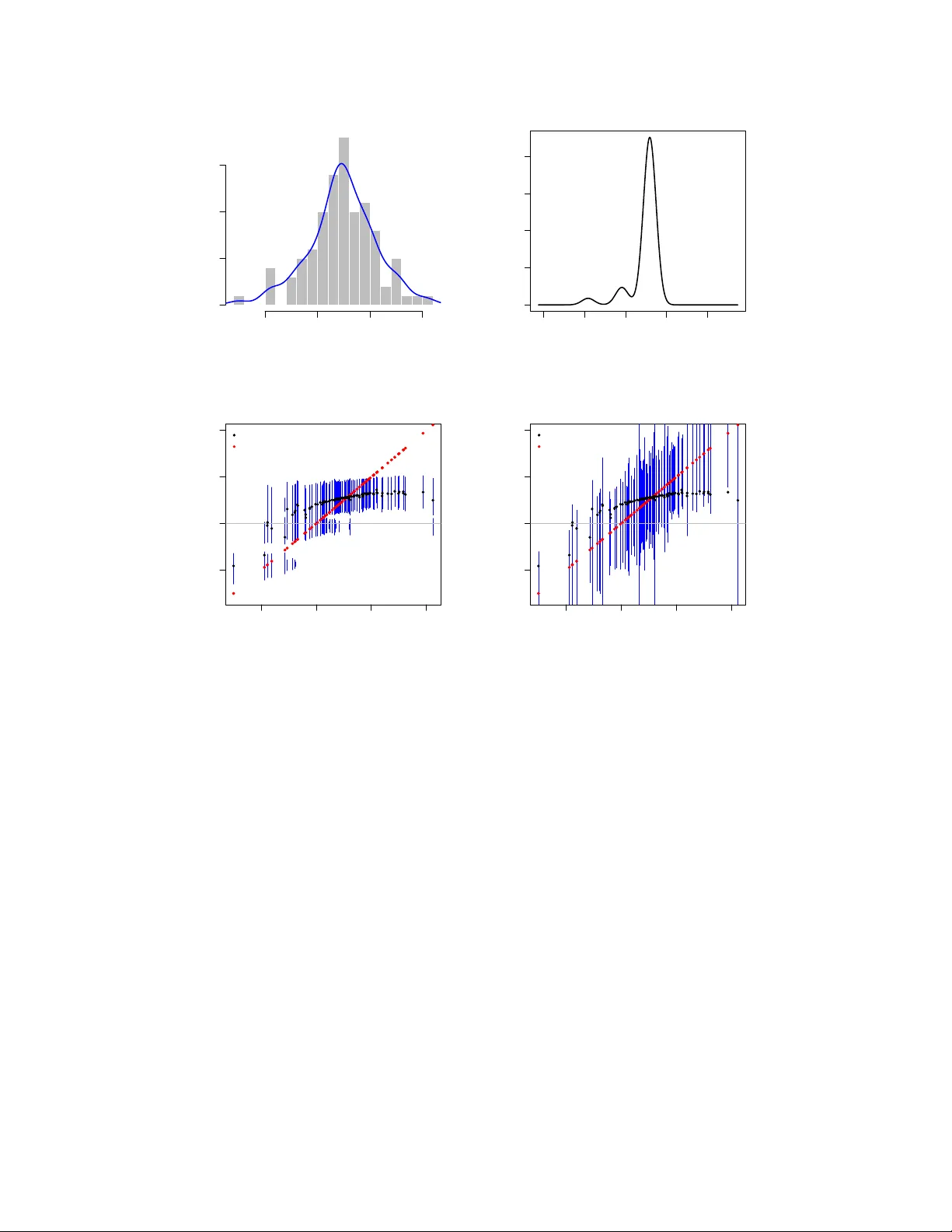
Empirical Ba y es Estimation and Inference via Smo oth Nonparametric Maxim um Lik eliho o d T aeh yun Kim ∗ Departmen t of Statistics, Colum bia Univ ersit y and Bo dhisattv a Sen † Departmen t of Statistics, Colum bia Univ ersit y Marc h 31, 2026 Abstract The empirical Ba yes g -mo deling approac h via the nonparametric maxim um like liho o d estimator (NPMLE) is widely used for large-scale estimation and inference in the normal means problem, y et theoretical guarantees for uncertaint y quan tiﬁcation remain scarce. A key obstacle is that the NPMLE of the mixing distribution is necessarily discrete, which yields discrete p osterior credible sets and a deconv olution rate that is logarithmic. W e address both limitations by studying a hierarchical Gaussian smo othing la y er that restricts the mixing distribution to a Gaussian lo cation mixture. The resulting smo oth NPMLE is computed by solving a conv ex optimization problem and inherits the near-parametric denoising p erformance of the classical NPMLE. F or decon volution it ac hieves a p olynomial rate of conv ergence which w e sho w is asymptotically minimax ov er the corresp onding class. The estimated smo oth p osteriors con verge to the true p osteriors at the same polynomial rate in w eigh ted total v ariation distance. When the mo del is missp eciﬁed, the smo oth NPMLE conv erges to the Kullback-Leibler pro jection of the true marginal densit y on to the mo del class at a nearly parametric rate, and the p olynomial deconv olution and p osterior con vergence rates carry ov er to this pseudo-true target. Building on this smo oth p osterior, we characterize optimal marginal co verage sets: the shortest set-v alued rules achieving a prescrib ed marginal co verage probabilit y . Plug-in empirical Bay es marginal cov erage sets based on the smo oth NPMLE achiev e asymptotically exact co verage at a p olynomial rate and conv erge to the oracle optimal set in exp ected length. All results extend to heteroscedastic Gaussian observ ations. W e also study iden tiﬁability of the prop osed mo del and show that the largest Gaussian comp onent of the prior is identiﬁable, and provide a consistent estimator and a ﬁnite-sample upp er conﬁdence b ound for it. ∗ E-mail: tk3036@colum bia.edu † The author gratefully ac kno wledges support from NSF grants DMS-2311062 and DMS-2515520. E-mail: b.sen@colum bia.edu 1 K eywor ds: Decon v olution, denoising, g -mo deling, heteroscedastic errors, hierarchical Gaus- sian lo cation mixture mo del, identiﬁabilit y , mo del missp eciﬁcation, optimal marginal co v er- age sets, p osterior distribution estimation. 1 In tro duction Consider the protot ypical normal lo cation mixture mo del: X i | θ i ind ∼ N ( θ i , 1) , and θ i iid ∼ G ∗ , for i = 1 , . . . , n, (1.1) where w e observe X 1 , . . . , X n , the θ 1 , . . . , θ n are laten t (unobserved), and the mixing distri- bution (or “prior”) G ∗ is unknown and b elongs to P ( R ) , the collection of all probability measures on R . Mo del ( 1.1 ) is a cen tral workhorse in empirical Ba yes, and it has b een studied extensiv ely from several complemen tary p ersp ectiv es. The main ob jectiv es pursued in this setting include: (i) estimation of the marginal densit y of the observ ations { X i } n i =1 [ 63 , 27 , 64 , 53 , 57 ]; (ii) denoising { X i } n i =1 to estimate/predict { θ i } n i =1 [ 8 , 35 , 53 , 57 , 28 ]; (iii) estimation of the mixing distribution G ∗ itself [ 24 , 57 ]; and (iv) uncertain ty quantiﬁcation and inference for { θ i } n i =1 [ 47 , 42 , 35 , 2 ]. A common approach to empirical Ba y es estimation pro ceeds via g -mo deling : one estimates the unkno wn mixing distribution G ∗ directly from the data and then plugs this estimate into do wnstream pro cedures [ 41 , 23 , 35 ]. A widely used c hoice is the nonparametric maximum lik eliho o d estimator (NPMLE) [ 38 ], deﬁned as the maximizer of the marginal lik eliho o d of { X i } n i =1 o ver P ( R ) . It is w ell-known that the NPMLE exhibits strong theoretical and empirical p erformance—it ac hieves near-parametric conv ergence rates (under suitable conditions) for marginal density estimation and for denoising in the normal means problem; see e.g., [ 64 , 53 , 57 ]. Building on the close connection b etw een the marginal density and the p osterior mean E G ∗ [ θ i | X i ] —the Bay es-optimal predictor of θ i under squared error loss—Jiang and Zhang [ 35 ] sho w that the plug-in p osterior mean based on the NPMLE attains nearly parametric regret rates under mild conditions; related results app ear in Saha and Gun tub o yina [ 53 ], Soloﬀ et al. [ 57 ], etc. Despite these strengths, the NPMLE is not w ell suited for de c onvolution , i.e., reco vering G ∗ itself from the noisy observ ations. I n particular, conv ergence of the NPMLE to G ∗ can b e logarithmically slow (see e.g., Theorem 11 of Soloﬀ et al. [ 57 ] ). Such slo w rates reﬂect the in trinsic ill-p osedness of deconv olution and are, in fact, minimax-optimal ov er Sob olev classes [ 13 , 26 ]. A further limitation is that the NPMLE is necessarily discrete [ 43 , 35 , 54 ], whic h can b e undesirable when the true G ∗ is smo oth. This discreteness also complicates inference for { θ i } n i =1 : the implied plug-in p osterior for eac h θ i giv en X i is discrete, leading to p osterior credible sets with an inheren tly discrete structure. T o address these limitations, it is natural to in vok e the “ b et on smo othness ” principle [ 24 , 25 ], whic h recommends restricting attention to suitably smo oth classes of mixing distributions for G ∗ . Several inﬂuential prop osals follo w this philosophy . Efron [ 24 ] , for example, mo dels the prior density within a (quasi-)parametric exp onential-family form using a natural spline basis, pro ducing a smo oth and often accurate estimate of G ∗ . Stephens [ 58 ] instead p osit Gaussian scale-mixture priors (typically with a mo de at zero) to obtain stabilized, smo othed 2 p osterior distributions. Bovy et al. [ 6 ] prop ose Extr eme De c onvolution (XD), which mo dels the unkno wn prior as a ﬁnite Gaussian lo cation-scale mixture, i.e., G ∗ is assumed to ha v e densit y g given by g ( · ) = K X k =1 w k ϕ τ k ( · − ξ k ) , (1.2) where ϕ σ denotes the N (0 , σ 2 ) density . The parameters { ( w k , ξ k , τ 2 k ) } K k =1 are typically ﬁt via the Exp ectation-Maximization (EM) algorithm. XD has b een eﬀective in astronomy applications [ 1 ], but it has tw o key limitations. Because the ﬁnite-mixture likelihoo d is non-con v ex, EM can con verge to lo cal rather than global maxima. In addition, the num b er of mixture comp onents K m ust b e chosen, and o ver- or under-sp ecifying this choice can induce missp eciﬁcation error, with limited theory for the resulting end-to-end pro cedure. Motiv ated b y the b et on smo othness principle, we introduce an additional latent lay er in ( 1.1 ) that enforces a con trolled amount of smo othing on the mixing distribution. Sp eciﬁcally , we consider the follo wing hierarchical normal lo cation mixture mo del: for i = 1 , . . . , n , X i | θ i ind ∼ N ( θ i , 1) , θ i | ξ i ind ∼ N ( ξ i , c 2 ∗ ) , ξ i iid ∼ H ∗ , (1.3) where, for now, c ∗ ≥ 0 is treated as kno wn and H ∗ ∈ P ( R ) is an unkno wn distribution. (In later sections w e relax the assumption that c ∗ is kno wn.) Under ( 1.3 ) , the marginal law of θ i is a Gaussian con volution of H ∗ , so the mixing distribution in ( 1.1 ) can b e written as G ∗ = H ∗ ⋆ N (0 , c 2 ∗ ) , (1.4) where ⋆ denotes con volution on R . When c ∗ = 0 , ( 1.3 ) reduces to the original normal lo cation mixture mo del ( 1.1 ) ; when c ∗ > 0 , it restricts G ∗ to a smo oth sub class obtained b y Gaussian smo othing. Equiv alently , the marginal densit y of θ i tak es the form g H ∗ ( θ ) := Z ϕ c ∗ ( θ − ξ ) d H ∗ ( ξ ) , θ ∈ R . (1.5) In this pap er w e estimate H ∗ via the NPMLE, deﬁned as an y maximizer “ H n ∈ argmax H ∈P ( R ) n X i =1 log f H ( X i ) , (1.6) where f H is the marginal densit y of X i induced b y H under ( 1.3 ), i.e., f H ( x ) := Z ϕ ( x − θ ) g H ( θ ) d θ = Z ϕ σ ∗ ( x − ξ ) d H ( ξ ) , x ∈ R . (1.7) where σ 2 ∗ := 1 + c 2 ∗ . Unlik e the XD approach in ( 1.2 ) , computing the NPMLE “ H n amoun ts to solving a c onvex optimization problem, alb eit inﬁnite-dimensional; this can b e easily approximated b y a ﬁnite- dimensional con v ex problem and eﬃciently solved using oﬀ-the-shelf conv ex programming metho ds that are eﬀectively tuning-free [ 40 , 39 ]. Moreov er, “ H n induces a natural plug-in estimator of the smo oth prior densit y g H ∗ in ( 1.5 ): g “ H n ( · ) := Z ϕ c ∗ ( · − ξ ) d “ H n ( ξ ) , (1.8) 3 −6 −4 −2 0 2 4 6 0.00 0.05 0.10 0.15 0.20 0.25 0.30 Classical NPMLE θ Density T rue Est. −6 −4 −2 0 2 4 6 0.00 0.05 0.10 0.15 0.20 0.25 0.30 Smooth NPMLE θ Density T rue Est. −6 −4 −2 0 2 4 6 0.0 0.1 0.2 0.3 0.4 0.5 0.6 Posterior distrib ution with Smooth NPMLE θ Density T rue, x = −2 Est., x = −2 T rue, x = 2 Est., x = 2 Figure 1: W e consider G ∗ = N ( − 2 , 1) / 2 + N (2 , 1) / 2 in ( 1.1 ) (equiv alently , H ∗ = δ − 2 / 2 + δ 2 / 2 and c ∗ = 1 in ( 1.3 ) ); here δ x denotes the Dirac delta measure at x . The classical (discrete) NPMLE (obtained from mo del ( 1.1 ) ) and the smo oth NPMLE g c H n (from ( 1.8 ) ) are computed using n = 1000 observ ations and sho wn in the left and cen ter plots along with the true prior density g H ∗ . F or the smo oth NPMLE, c ∗ is also estimated using the neighborho o d procedure describ ed in Section 5 . The true p osterior densities at x = ± 2 and the estimated posterior densities based on the smo oth NPMLE are sho wn in the righ tmost plot. whic h is itself a Gaussian lo cation mixture. This construction coincides with the smo oth NPMLE of Magder and Zeger [ 44 ] (see also [ 15 , 54 ]). Since “ H n has at most n supp ort p oin ts [ 43 ], it automatically yields a ﬁnite Gaussian lo cation-mixture prior, but without the non-con v exity and comp onen t-selection issues inherent to XD. A primary task in empirical Bay es is to denoise the observ ations X i to estimate/predict the laten t eﬀects θ i . Under squared error loss, the oracle decision rule is the p osterior mean E g H ∗ [ θ i | X i ] , and the g -mo deling approach replaces the unkno wn prior density g H ∗ in ( 1.5 ) b y the plug-in estimator g “ H n in ( 1.8 ) . A key adv an tage of the hierarc hical normal-normal model ( 1.3 ) is that it preserv es the tractable structure of the p osterior mean through the Gaussian mixture representation ( 1.7 ) . Consequently , E g H ∗ [ θ i | X i ] is a conv ex combination of the raw observ ation X i and E H ∗ [ ξ i | X i ] (see ( 2.3 ) ), making the plug-in empirical Ba y es estimate straightforw ard to compute. F urther, the strong theoretical guaran tees for denoising via the classical NPMLE [ 35 , 53 ] carry o ver without loss to our smo oth g -mo deling framew ork; see Section 2.1 . Moreo ver, we sho w that g “ H n con verg es to g H ∗ at a fast p olynomial rate (Theorem 2.1 ), in sharp contrast to the logarithmically slow b eha vior of the classical NPMLE under the original mo del ( 1.1 ) [ 57 ]. W e also show that this p olynomial rate is asymptotically minimax optimal (Theorem 2.2 ). F urthermore, we show that the p osterior distribution estimated using the smo oth NPMLE con v erges to the true p osterior distribution at a p olynomial rate (Theorem 2.3 ). W e illustrate the adv an tages of using the smo oth NPMLE in Figures 1 and 2 . Note that the t wo-component normal mixture prior in Figure 1 can b e expressed as g H ∗ in ( 1.5 ) with c ∗ = 1 . In con trast, the Laplace prior in Figure 2 cannot b e written as g H ∗ unless c ∗ = 0 . Nev ertheless, the Laplace densit y can b e approximated by a mixture of normals, and the smo oth NPMLE can still pro vide a reasonable approximation to the true prior density . More generally , Gaussian mixtures are dense in broad classes of con tinuous probability densities, so smo oth NPMLEs can approximate a wide range of true prior distributions. 4 −4 −2 0 2 4 0.0 0.1 0.2 0.3 0.4 0.5 0.6 Classical NPMLE θ Density T rue Est. −4 −2 0 2 4 0.0 0.1 0.2 0.3 0.4 0.5 0.6 Smooth NPMLE θ Density T rue Est. −4 −2 0 2 4 0.0 0.1 0.2 0.3 0.4 0.5 0.6 Marginal densities X Density T rue Est. Figure 2: The setup is the same as in Figure 1 , except that the true prior is G ∗ = Laplace (0 , 1) . The true marginal densit y of the observ ations and the estimated marginal density based on the smo oth NPMLE are sho wn in the righ tmost plot. F or the smooth NPMLE, c ∗ is estimated using the neigh b orho o d procedure describ ed in Section 5 . While the true prior densities used in Figures 1 and 2 are smo oth (except at θ = 0 for G ∗ = Laplace (0 , 1) ), the (nonsmo oth) classical NPMLE (based on mo del ( 1.1 ) ) is discrete and do es not capture the shap e of the underlying true prior v ery well. The right panel of Figure 2 shows that the estimated marginal densit y f “ H n , constructed with the estimated c ∗ obtained by the neigh b orho od pro cedure describ ed in Section 5 , still approximates the true marginal density quite well. In this case, the true marginal densit y is not included in the mo del class F := { f H : H ∈ P ( R ) } , where f H is deﬁned in ( 1.7 ) . When the mo del is missp eciﬁed, we show, under a technical compact supp ort restriction on the mo del class, that f “ H n con v erges to the pseudo-true marginal density at a nearly parametric rate up to logarithmic factors, in a divergence inspired by the Hellinger distance (Theorem 2.4 ). Here, the pseudo-true marginal density is the Kullback-Leibler pro jection of the true marginal densit y onto the mo del class. F urther, the smo oth NPMLE g “ H n con v erges to the pseudo-true prior density at a p olynomial rate under mild conditions (Theorem 2.5 ). The estimated p osterior density also con verges to the pseudo-true p osterior densit y in weigh ted total v ariation distance at a p olynomial rate up to logarithmic factors. While empirical Bay es metho ds hav e b een extensive ly developed for predicting the laten t eﬀects { θ i } n i =1 [ 33 , 35 , 53 , 57 ], comparativ ely less is known ab out uncertain t y quantiﬁcation in this setting [ 47 , 34 , 2 ]. An adv an tage of introducing a smo oth prior through ( 1.3 ) is that it yields a tractable route to conﬁdence/prediction set construction based on the smo oth NPMLE, whic h is considerably more delicate under the original mo del ( 1.1 ) . In this pap er, w e fo cus on the notion of mar ginal cov erage: a prediction set J i ≡ J i ( X i ) is said to ha ve (1 − β ) marginal co verage for θ i if P H ∗ ( θ i ∈ J i ) ≥ 1 − β , (1.9) where the probabilit y is taken with resp ect to the joint law of ( X i , θ i ) in ( 1.3 ) . Marginal co verage is natural in empirical Ba y es problems b ecause laten t eﬀects are mo deled as dra ws from a common prior [ 47 , 2 ]; moreov er, av erage cov erage is more relev an t in many applications than cov erage for any sp eciﬁc eﬀect [ 30 , 29 ]. Marginal cov erage ( 1.9 ) is also less stringen t than requiring J i to b e a (conditional) frequentist conﬁdence in terv al for eac h 5 ﬁxed θ i (i.e., the usual (1 − β ) normal-theory in terv al S i = X i ± z 1 − β / 2 ) or an exact Bay esian credible set (i.e., the (1 − β ) highest p osterior density set). Despite its imp ortance, there has not b een a rigorous study of optimal marginal cov erage sets in a nonparametric setting; in Section 3 w e characterize the form of these optimal marginal cov erage sets. Our approach targets marginal co verage sets that are optimal in exp ected length among all pro cedures that satisfy ( 1.9 ) . W e sho w that the optimal construction is closely related to highest p osterior densit y (HPD) sets. In particular, for each ﬁxed x , the HPD set I x ( k ( x )) := { θ ∈ R : π H ∗ ( θ | x ) ≥ k ( x ) } minimizes length among all cr e dible sets with the same p osterior con ten t, where π H ∗ ( · | x ) denotes the p osterior density of θ i giv en X i = x . Our key observ ation is that if one replaces the data-dep endent threshold k ( x ) by a c onstant threshold k ∗ c hosen so that ( 1.9 ) holds, then the resulting set I ∗ ( x ) := { θ ∈ R : π H ∗ ( θ | x ) ≥ k ∗ } is optimal, in terms of exp ected length, among all marginal co verage sets (Theorem 3.1 ). W e note that this observ ation holds for general lik eliho o d functions b ey ond the normal family in ( 1.1 ) and for arbitrary mixing distributions (cf. Jiang [ 34 ]). Our next goal is to construct empiric al Bayes pr e diction sets J i ≡ J i ( X 1 , . . . , X n ) that (appro ximately) satisfy ( 1.9 ) for eac h i , and target the oracle set I ∗ ( X i ) , while allo wing J i to b orro w strength across co ordinates through its dep endence on all observ ations. A practical c hallenge under the original mo del ( 1.1 ) is that when I ∗ ( x ) is estimated b y plugging in the classical NPMLE, the implied p osterior is discrete, and the resulting prediction sets inherit this discreteness. In con trast, under the hierarc hical mo del ( 1.3 ) , the estimated smo oth prior g “ H n yields a smo oth p osterior density and hence natural (non-discrete) plug-in prediction sets. Using the p olynomial conv ergence of g “ H n , we show that the cov erage of the estimated optimal marginal cov erage set approaches (1 − β ) at a polynomial rate (Theorem 3.2 ). Moreo v er, we sho w that the exp ected length of the estimated optimal marginal cov erage set con v erges to that of I ∗ at a p olynomial rate (Theorem 3.3 ). In the normal lo cation mixture mo del ( 1.3 ) w e assume i.i.d. observ ations; in man y practical applications the observ ations exhibit heter o geneity (i.e., v arying noise levels) [ 1 , 5 , 57 ]. In Section 4 and App endix D , we discuss statistical prop erties of the smo oth NPMLE and extensions of optimal marginal cov erage sets to suc h heterogeneous settings. In particular, w e sho w that g “ H n still con v erges to g H ∗ at a p olynomial rate (Theorem D.2 ). Next w e discuss several practical issues surrounding the smo oth-prior form ulation and our prop osed marginal cov erage sets. First, the smo othing parameter c ∗ in ( 1.3 ) is t ypically unkno wn in applications, and the decomp osition G ∗ = H ∗ ⋆ N (0 , c 2 ∗ ) is not iden tiﬁable without additional structure: multiple pairs ( H ∗ , c ∗ ) can induce the same G ∗ . W e address this b y working with an identiﬁable target, namely the lar gest Gaussian c omp onent of G ∗ , denoted c 0 ; see ( 5.1 ) for a formal deﬁnition. W e prop ose t wo metho ds for estimation and inference on c 0 : a neigh b orho o d-based pro cedure in the spirit of Donoho [ 21 ] , and a split lik eliho o d ratio test of W asserman et al. [ 60 ] (see App endix F ). One ma y ask when a nonparametric empirical Ba yes analysis is warran ted as opp osed to a simpler parametric empirical Bay es mo del. W e formalize this question via the go o dness-of-ﬁt 6 test H 0 : H ∗ = δ a for some a ∈ R v ersus H 1 : not H 0 , (1.10) under whic h H 0 corresp onds to the parametric prior θ i iid ∼ N ( a, c 2 ∗ ) for some a ∈ R . If H 0 is not rejected, then parametric empirical Ba yes in terv als suc h as those of Morris [ 47 ] are w ell-motiv ated; if H 0 is rejected, there is less justiﬁcation for a Gaussian prior and it is natural to rely on nonparametric empirical Bay es metho ds. W e discuss implementing this test using the split likelihoo d ratio (SLR) metho d of W asserman et al. [ 60 ] in Section 6 (as w ell as generalized likelihoo d ratio tests (GLR T s) coupled with a parametric b o otstrap approac h in App endix G ). The full smo oth g -mo deling pro cedure for estimation and inference dev elop ed in this pap er is summarized in Algorithm 1 . Algorithm 1 W orkﬂo w for empirical Bay es estimation and inference via smo oth NPMLE Require: Observ ations { X i } n i =1 and target co verage lev el 1 − β 1: Compute an estimate ˆ c 0 of c 0 in ( 5.1 ) using the neighborho o d pro cedure in Section 5 2: Compute the NPMLE “ H n in ( 1.6 ) using ˆ c 0 3: F orm the smo oth NPMLE g “ H n ( · ) in ( 1.8 ) and p osterior densit y π “ H n ( · | X i ) in ( 2.16 ) 4: Solve ( 3.12 ) for the threshold ˆ k B n for the optimal marginal co verage set Output I: The empirical Bay es p osterior means { ˆ θ i } n i =1 as describ ed in ( 2.4 ) and ( 2.5 ) Output I I: The empirical Bay es marginal cov erage sets { ˆ I B n ( X i ) } n i =1 in ( 3.11 ) The rest of the pap er is organized as follows. Section 2 establishes statistical prop erties of the smo oth NPMLE for denoising, deconv olution, estimation of p osterior densit y , and under mo del missp eciﬁcation. Section 3 develops optimal marginal cov erage sets and studies the theoretical properties of their empirical Ba yes counterparts. In Section 4 we study extensions to heteroscedastic versions of ( 1.3 ) . Section 5 addresses identiﬁabilit y in the hierarchical mo del ( 1.3 ) . Section 6 introduces go o dness-of-ﬁt pro cedures for testing ( 1.10 ) . Section 7 presen ts a real-data example illustrating the smo oth NPMLE and optimal marginal co v erage sets. W e end with a brief discussion and some op en directions in Section 8 . All pro ofs of the main results, further discussions, additional illustrations and n umerical exp erimen ts, and practical implemen tation details for the smo oth NPMLE are given in the App endix. Throughout, we write x ≳ p,q y or x ≲ p,q y to mean that x ≥ C p,q y or x ≤ C p,q y for a constan t C p,q > 0 dep ending only on the parameters p and q . W e write P ( A ) for the collection of all probability measures on A ⊆ R . Unless otherwise stated, let E H and P H denote the exp ectation and probability under mo del ( 1.3 ) with ξ i iid ∼ H ∈ P ( R ) . Deﬁne X (1) := min i X i and X ( n ) := max i X i to b e the minim um and maxim um of the sample. 2 Statistical prop erties of smo oth NPMLE In this section, w e inv estigate statistical prop erties of the smo oth NPMLE g “ H n in ( 1.8 ) under the hierarc hical mo del ( 1.3 ) . Supp ose for now that c ∗ in ( 1.3 ) is kno wn. A direct Gaussian calculation yields: θ i | X i , ξ i ∼ N ( α ∗ X i + (1 − α ∗ ) ξ i , α ∗ ) , for i = 1 , . . . , n, (2.1) 7 where (recall σ 2 ∗ := c 2 ∗ + 1 ) α ∗ := c 2 ∗ σ 2 ∗ = c 2 ∗ c 2 ∗ + 1 . (2.2) The quan tit y α ∗ ∈ (0 , 1) measures the eﬀectiv e smo othing induced by c ∗ > 0 , and satisﬁes α ∗ ↑ 1 as c ∗ → ∞ . If H ∗ w ere kno wn, the oracle p osterior mean of θ i w ould b e: ˆ θ ∗ i := E H ∗ [ θ i | X i ] = E H ∗ [ E [ θ i | X i , ξ i ] | X i ] = E H ∗ [ α ∗ X i + (1 − α ∗ ) ξ i | X i ] = α ∗ X i + (1 − α ∗ ) E H ∗ [ ξ i | X i ] = α ∗ X i + (1 − α ∗ ) ˆ ξ ∗ i (2.3) where ˆ ξ ∗ i := E H ∗ [ ξ i | X i ] is the oracle p osterior mean of ξ i giv en X i . In our smo oth g -mo deling approach, we estimate H ∗ b y the NPMLE “ H n deﬁned in ( 1.6 ) . Plugging “ H n in to ( 1.5 ) yields the smo oth NPMLE g “ H n in ( 1.8 ) . Moreov er, as in ( 2.3 ) , the hierarc hical normal-normal structure allo ws the oracle p osterior mean to b e expressed as a con vex combination of X i and E H ∗ [ ξ i | X i ] . The empirical Bay es estimate of ˆ θ ∗ i is then giv en b y ˆ θ i := E “ H n [ θ i | X i ] = α ∗ X i + (1 − α ∗ ) E “ H n [ ξ i | X i ] = α ∗ X i + (1 − α ∗ ) ˆ ξ i , (2.4) where ˆ ξ i := E “ H n [ ξ i | X i ] = R ξ ϕ σ ∗ ( X i − ξ ) d “ H n ( ξ ) f “ H n ( X i ) (2.5) is the empirical Ba y es estimate of the oracle p osterior mean of ξ i giv en X i . This represen- tation mak es p osterior mean computation simple in the normal-normal setting. Although computing “ H n in v olves an inﬁnite-dimensional optimization problem, it can b e accurately appro ximated by a ﬁnite-dimensional con vex program on a ﬁne grid [ 40 , 57 ]. Note that “ H n is discrete with at most n atoms [ 43 ], so the integral in ( 2.5 ) reduces to a ﬁnite sum; the empirical Ba y es p osterior means are esp ecially easy to compute in our setting. 2.1 Denoising One of the main uses of the estimated prior g “ H n is in denoising: constructing accurate empirical Ba y es (EB) p osterior means. Under the hierarc hical mo del ( 1.3 ) , the laten t v ariable of interest ξ i ∼ H ∗ is ﬁrst p erturb ed to θ i b y Gaussian noise of v ariance c 2 ∗ , and then observ ed through X i with unit noise. Equiv alently , X i = ξ i + ( θ i − ξ i ) + ( X i − θ i ) ⇒ X i | ξ i ∼ N ( ξ i , σ 2 ∗ ) , σ 2 ∗ := 1 + c 2 ∗ . Th us, from the p ersp ectiv e of estimating ξ i , the mo del reduces to a classical Gaussian lo cation mixture with known v ariance σ 2 ∗ . This reduction allo ws us to leverage the well-dev elop ed EB/NPMLE theory for normal mixtures. W e quan tify EB performance via the (excess) mean-squared error relativ e to the ora- cle Bay es rule. Since ˆ θ ∗ i = E H ∗ [ θ i | X i ] is the L 2 -pro jection of θ i on to σ ( X i ) , the Pythagorean/orthogonalit y iden tity yields R n ( ˆ θ , ˆ θ ∗ ) := E ñ 1 n n X i =1 ( θ i − ˆ θ i ) 2 ô − E ñ 1 n n X i =1 ( θ i − ˆ θ ∗ i ) 2 ô = E ñ 1 n n X i =1 ( ˆ θ i − ˆ θ ∗ i ) 2 ô . (2.6) 8 Moreo ve r, the p osterior mean formulas ( 2.3 ) – ( 2.4 ) imply that estimating/predicting θ i is essen tially equiv alen t to estimating ξ i : R n ( ˆ θ , ˆ θ ∗ ) = E ñ (1 − α ∗ ) 2 n n X i =1 ( ˆ ξ i − ˆ ξ ∗ i ) 2 ô , (2.7) where ˆ ξ ∗ i := E H ∗ [ ξ i | X i ] and ˆ ξ i := E “ H n [ ξ i | X i ] . Equation ( 2.7 ) is particularly reve aling: up to the explicit factor (1 − α ∗ ) 2 = (1 + c 2 ∗ ) − 2 , the excess Ba yes risk for estimating θ i is exactly the excess Bay es risk for predicting ξ i in the induced Gaussian mixture mo del. Th us, the additional Gaussian p erturbation in ( 1.3 ) do es not create a new denoising diﬃculty; it simply reduces the problem to a classical EB normal-mixture problem with noise level σ 2 ∗ . Under the hierarc hical mo del ( 1.3 ), we hav e X i | ξ i ind ∼ N ( ξ i , σ 2 ∗ ) , and ξ i iid ∼ H ∗ , for i = 1 , . . . , n, and the denoising problem of { ξ i } n i =1 via { ˆ ξ i } n i =1 is well-understoo d in the literature [ 35 , 53 , 57 ]. F or a nonempty set S ⊆ R , deﬁne d S : R → [0 , ∞ ) by d S ( x ) := inf u ∈ S | x − u | f or x ∈ R . (2.8) That is, d S ( x ) is the distance from x to the set S . Also, for S ⊆ R , we let S σ ∗ := { x : d S ( x ) ≤ σ ∗ } . (2.9) Th us, S σ ∗ is the σ ∗ enlargemen t of the set S . F or ev ery H ∈ P ( R ) , every non-empty compact set S ⊆ R and every M ≥ p 10 σ 2 ∗ log n , let ϵ n ( M , S, H ) b e deﬁned via ϵ 2 n ( M , S , H ) := V ol ( S σ ∗ ) M n (log n ) 3 / 2 + (log n ) inf p ≥ 1 log n Å 2 µ p ( d S , H ) M ã p (2.10) where S σ ∗ is deﬁned in ( 2.9 ) and µ p ( d S , H ) is the p th moment of d S ( ξ ) under ξ ∼ H : µ p ( d S , H ) :=  Z R ( d S ( ξ )) p d H ( ξ )  1 /p for p > 0 . Heuristically , ϵ 2 n ( M , S , H ∗ ) captures the eﬀectiv e statistical complexit y of the Gaussian mixture mo del induced by ( 1.3 ) . The ﬁrst term dep ends on the size of the σ ∗ -enlarged supp ort S σ ∗ , while the second term measures ho w m uch mass of H ∗ lies far from S . Com bining ( 2.7 ) with Theorems 7 and 9 of Soloﬀ et al. [ 57 ] yields that, for an y ﬁxed M ≥ p 10 σ 2 ∗ log n and compact S ⊆ R , R n ( ˆ θ , ˆ θ ∗ ) ≲ c ∗ ϵ 2 n ( M , S, H ∗ )(log n ) 3 . In particular, when H ∗ has suﬃciently simple eﬀective supp ort—for example, ﬁnite supp ort, compact supp ort, or tails that can b e well-appro ximated by a compact set S —the quan tity ϵ 2 n ( M , S, H ∗ ) is nearly of order n − 1 up to logarithmic factors, so the smo oth NPMLE ac hiev es almost parametric excess Bay es risk. Although this conclusion is inherited from existing Gaussian-mixture NPMLE theory , it is an imp ortant b enchmark for our hierarc hical 9 mo del: the smo othing device used to deﬁne g “ H n do es not sacriﬁce classical EB denoising p erformance. Rather, it preserves near-oracle denoising guarantees while also laying the foundation for the sharp er decon volution and uncertaint y quantiﬁcation results developed in the follo wing sections. Using Theorem 7 of Soloﬀ et al. [ 57 ] , it can b e sho wn that the rate function ϵ 2 n ( M , S , H ∗ ) also upper b ounds the squared Hellinger distance H 2 ( f “ H n , f H ∗ ) in expectation, where H 2 ( f , g ) := 1 2 R ( √ f − √ g ) 2 . Thus, f H ∗ , the true marginal density of X i , can b e recov ered, in squared Hellinger distance, at nearly the parametric ( n − 1 ) rate, under suitable assumptions on H ∗ ; w e state this result formally in Theorem A.1 for completeness. 2.2 Decon volution Next, w e consider the problem of estimating g H ∗ in ( 1.5 ) , whic h is the true prior density of θ i under the hierarchical mo del ( 1.3 ) . It is natural to ask how well the plug-in estimator g “ H n in ( 1.8 ) estimates g H ∗ . As mentioned earlier, in estimating f H ∗ , whic h is the true marginal densit y of X i , the plug-in estimator f “ H n ac hieves almost parametric rates under suitable assumptions on H ∗ . In con trast, the deconv olution error b etw een “ H n and H ∗ is upp er b ounded by the quite slo w logarithmic rate in 2-W asserstein distance (see Theorem 11 of Soloﬀ et al. [ 57 ] ). In fact, the logarithmic rate is minimax optimal o ver Sob olev classes in the classical deconv olution setting, where no additional hierarc hical structure is a v ailable [ 26 , 46 ]. Our setting diﬀers fundamen tally: under the hierarc hical mo del with c ∗ > 0 , an additional smo othing eﬀect links the estimation of g H ∗ to the near-parametric estimation of f H ∗ , allo wing p olynomial rates of recov ery in L 2 distance; see Theorem 2.1 b elo w. Our result is expressed in terms of the rate function ϵ 2 n ( M , S, H ∗ ) in ( 2.10 ) , whic h also controls the squared Hellinger accuracy H 2 ( f “ H n , f H ∗ ) . Theorem 2.1. Supp ose that ( 1.3 ) holds for al l i = 1 , . . . , n wher e c ∗ > 0 . R e c al l that α ∗ := c 2 ∗ /σ 2 ∗ (se e ( 2.2 ) ) wher e σ 2 ∗ = c 2 ∗ + 1 . L et “ H n b e any solution of ( 1.6 ). F or any ﬁxe d M ≥ p 10 σ 2 ∗ log n and a nonempty, c omp act set S ⊆ R , deﬁne ϵ n := ϵ n ( M , S , H ∗ ) as in ( 2.10 ) . Supp ose further that ϵ n = o (1) . Then, ∥ g “ H n − g H ∗ ∥ 2 L 2 ≲ c ∗ t 2 ϵ 2 α ∗ n (2.11) for al l t ≥ 1 , with pr ob ability at le ast 1 − 2 n − t 2 . Mor e over, E H ∗ î ∥ g “ H n − g H ∗ ∥ 2 L 2 ó ≲ c ∗ ϵ 2 α ∗ n . (2.12) W e provide the pro of of Theorem 2.1 in App endix I.1 . The main ingredient in the pro of is the relation b et w een ∥ g “ H n − g H ∗ ∥ 2 L 2 and ∥ f “ H n − f H ∗ ∥ 2 L 2 via Planc herel’s theorem, together with the fact that ϵ 2 n ( M , S, H ∗ ) b ounds the rate of H 2 ( f “ H n , f H ∗ ) . F or instance, when g H ∗ is a smo oth density , suc h as a ﬁnite Gaussian mixture, our b ound implies p olynomial con vergence of g “ H n in L 2 -norm under the hierarc hical mo del ( 1.3 ) , in contrast to the logarithmic rates that are typical in classical Gaussian deconv olution (under broader and less structured assumptions). T o the b est of our knowledge, this is 10 the ﬁrst such p olynomial L 2 con v ergence result for the smo oth NPMLE in our hierarc hical Gaussian smo othing framew ork. As mentioned earlier, w e can choose M and S so that ϵ 2 n ( M , S, H ∗ ) ≍ n − 1 , up to logarithmic multiplicativ e factors, under v arious assumptions on H ∗ . In such cases, the con v ergence rate ( 2.12 ) b ecomes n − α ∗ , up to logarithmic factors. When g H ∗ is suﬃciently smo oth and c ∗ > 0 is large, the gain from smo othing b ecomes substan tial. In the extreme case where c ∗ is large and α ∗ ≈ 1 , g “ H n ac hieves an almost parametric rate of conv ergence, up to logarithmic factors. This aligns with our observ ation that the smo oth NPMLE g “ H n appro ximates g H ∗ w ell in the center panel of Figure 1 . In fact, it can b e shown that the con vergence rate n − α ∗ is asymptotically minimax, up to logarithmic factors, for estimating the prior densit y g H ∗ with resp ect to squared L 2 -risk, under the additional smo othness implied b y ( 1.5 ) . It has b een known that the minimax rate of deconv olution for a Gaussian error is logarithmic ov er the Sob olev class G r,L [ 26 , 46 ], whic h is the collection of all densities g whose F ourier transform φ g satisﬁes the follo wing condition: G r,L := n g is a p df on R : Z | φ g ( t ) | 2 | t | 2 r d t ≤ 2 π L o for r , L > 0 . Ho wev er, note that the true prior density g H ∗ = H ∗ ⋆ N (0 , c 2 ∗ ) in ( 1.5 ) is sup ersmo oth as its F ourier transform has exp onential tails as long as c ∗ > 0 . It implies that g H ∗ is contained in a more restricted class G r,ζ ,L ; exp compared to G r,L , which is deﬁned as the collection of all densities g satisfying G r,ζ ,L ; exp := n g is a p df on R : Z | φ g ( t ) | 2 exp( ζ | t | r ) d t ≤ 2 π L o . (2.13) Since | φ g H ∗ ( t ) | 2 = | φ H ∗ ( t ) | 2 e − c 2 ∗ t 2 , the Gaussian conv olution induces exp onen tial deca y . If H ∗ admits an L 2 densit y h , then φ H ∗ ∈ L 2 , and hence R | φ g H ∗ ( t ) | 2 e ζ | t | 2 dt < ∞ for all ζ ≤ c 2 ∗ . Th us g H ∗ b elongs to G 2 ,ζ ,L ;exp for ζ ≤ c 2 ∗ and suitable L . In particular, g H ∗ ∈ G r,ζ ,L ; exp with r = 2 and ζ = c 2 ∗ and L = ∥ h ∥ 2 L 2 , which corresp onds to the b oundary case of the sup ersmo oth scale when h ∈ L 2 ( R ) . It has b een kno wn that imp osing stronger smo othness conditions on the mixing distribution (i.e., g H ∗ ) as in G r,ζ ,L ;exp yields non-logarithmic rates; see, e.g., pages 44–45 in Meister [ 46 ] , Pensky and Vidako vic [ 50 ] , Butucea and T sybako v [ 10 , 11 ] and Butucea and Comte [ 9 ] . The following theorem c haracterizes the asymptotic lo wer b ound for the squared L 2 risk assuming r = 2 and ζ = c 2 ∗ . The pro of of Theorem 2.2 is giv en in App endix I.2 . Theorem 2.2. L et r = 2 and ζ = c 2 ∗ in ( 2.13 ) . Then lim inf n →∞ inf ˆ g n sup g ∈G r,ζ,L ; exp E g  ∥ ˆ g n − g ∥ 2 L 2  ψ − 2 n ≥ L, wher e E g denotes exp e ctation when X i = θ i + Z i , θ i iid ∼ g ∈ G r,ζ ,L ; exp , Z i iid ∼ N (0 , 1) , and θ i and Z i ar e indep endent for i = 1 , . . . , n , and the inﬁmum is over al l me asur able functions b ase d on the data X 1 , . . . , X n . Her e, the r ate ψ n is deﬁne d as: ψ 2 n := n − α ∗ (log n ) − C α ∗ . (2.14) for some ﬁxe d C > 1 . 11 Recall that α ∗ = c 2 ∗ / (1 + c 2 ∗ ) , so the rate interpolates b etw een the parametric regime ( c 2 ∗ → ∞ ) and the severely ill-p osed regime ( c 2 ∗ → 0 ). The pro of of Theorem 2.2 adapts the construction of Butucea and T sybako v [ 11 ] to the b oundary case r = 2 , ζ = c 2 ∗ induced b y Gaussian con v olution in our hierarchical mo del. Theorems 2.1 and 2.2 imply that the smo oth NPMLE g “ H n is asymptotically minimax in G r,ζ ,C ; exp with r = 2 and ζ = c 2 ∗ up to logarithmic factors. 2.3 Estimation of p osterior densit y Our result on p olynomial conv ergence in the decon volution problem has an imp ortant implication for p osterior density estimation. While the p osterior distribution is central to ac hieving the goals of empirical Ba yes methods, m uch of the literature establishes theoretical guaran tees for only a few functionals such as the p osterior mean; it falls short of pro viding theoretical guaran tees for the p osterior distribution itself. Denote by π H ∗ ( θ | x ) := ϕ ( x − θ ) g H ∗ ( θ ) f H ∗ ( x ) , for θ , x ∈ R , (2.15) the p osterior density of θ i giv en X i = x where g H ∗ and f H ∗ are deﬁned in ( 1.5 ) and ( 1.7 ) , resp ectiv ely . With the plug-in estimators f “ H n and g “ H n based on the NPMLE ( 1.6 ) , w e hav e a natural plug-in estimator of π H ∗ ( · | x ) : π “ H n ( θ | x ) := ϕ ( x − θ ) g “ H n ( θ ) f “ H n ( x ) , for θ , x ∈ R . (2.16) Note that π “ H n ( · | x ) is smo oth as long as c ∗ > 0 . Our metric for quantifying the distance b et w een π “ H n and π H ∗ is the w eighted total v ariation distance: wTV( π “ H n , π H ∗ ) := Z TV( π “ H n ( · | x ) , π H ∗ ( · | x )) f H ∗ ( x ) d x. (2.17) Here, TV ( f , g ) = 1 2 R | f ( t ) − g ( t ) | d t denotes the usual total v ariation distance b etw een densities f and g . It can b e sho wn that wTV( π “ H n , π H ∗ ) ≤ TV( f “ H n , f H ∗ ) + TV( g “ H n , g H ∗ ) (see the pro of of Theorem 2.3 ). Th us, the quality of the p osterior approximation dep ends on ho w well the estimated marginal density f “ H n and the estimated prior density g “ H n appro ximate f H ∗ and g H ∗ , resp ectively . In the follo wing theorem, we provide the rate of con v ergence of π “ H n ( · | · ) to π H ∗ ( · | · ) in the w eigh ted total v ariation distance ( 2.17 ) . T o the b est of our knowledge, this is the ﬁrst such result for this estimation metho d that pro vides a p olynomial rate of con vergence for the p osterior densit y . This explains wh y π “ H n ( · | x ) appro ximates π H ∗ ( · | x ) w ell in the righ tmost panel of Figure 1 . W e pro vide the pro of of Theorem 2.3 in App endix I.3 . Theorem 2.3. Supp ose that ( 1.3 ) holds for al l i = 1 , . . . , n , wher e c ∗ > 0 . L et “ H n b e any solution of ( 1.6 ). F or any ﬁxe d M ≥ p 10 σ 2 ∗ log n and a nonempty, c omp act set S ⊆ R , deﬁne ϵ n := ϵ n ( M , S, H ∗ ) as in ( 2.10 ) . Supp ose further that ϵ n = o (1) . Then, E H ∗ î wTV( π “ H n , π H ∗ ) ó ≲ c ∗ p M V ol ( S σ ∗ ) ϵ α ∗ n . 12 Remark 2.1 (Compact supp ort) . Supp ose that H ∗ is supp orte d on a c omp act set S ∗ . Then we c an cho ose M = p 10 σ 2 ∗ log n and S = S ∗ so that ϵ 2 n ( M , S, H ∗ ) ≲ c ∗ V ol ( S σ ∗ ) n − 1 ( log n ) 2 . In this c ase, The or em 2.3 implies that E H ∗ î wTV( π “ H n , π H ∗ ) ó ≲ c ∗ p V ol ( S σ ∗ ) n − α ∗ / 2 ( log n ) 5 / 4 . 2.4 Mo del missp eciﬁcation So far, we hav e assumed that the observ ations X 1 , . . . , X n are distributed according to f H ∗ and the hierarchical mo del in ( 1.3 ) is well-speciﬁed. W e no w turn our attention to the case where mo del ( 1.3 ) is missp eciﬁed. That is, supp ose that ( 1.1 ) holds and X 1 , . . . , X n iid ∼ p G ∗ where the true marginal densit y of the observ ations, p G ∗ ( x ) := Z ϕ ( x − θ ) d G ∗ ( θ ) , x ∈ R , is not included in F := { f H : H ∈ P ( R ) } where f H is deﬁned in ( 1.7 ) . Note that f H dep ends on c ∗ implicitly . W e deﬁne the pseudo-true density f ˜ H ∈ F as the Kullback-Leibler (KL) pro jection of the true marginal densit y p G ∗ on to F : f ˜ H = argmin f ∈F KL( p G ∗ ∥ f ) , (2.18) where KL ( p ∥ q ) denotes the Kullbac k-Leibler (KL) divergence b etw een tw o probabilit y densit y functions p and q . When p G ∗ ∈ F , then f ˜ H = p G ∗ ; in general it is the element of F closest to p G ∗ in KL div ergence. Existence and uniqueness of f ˜ H are established in Theorem 2.4 . W e are interested in how w ell f “ H n estimated via the NPMLE in ( 1.6 ) con verge s to the pseudo-true densit y f ˜ H . In the case of missp eciﬁcation, Patilea [ 48 ] prop ose the div ergence H 2 0 ( f H , f ˜ H ) := 1 2 Z Ç  f H ( x ) f ˜ H ( x ) − 1 å 2 p G ∗ ( x ) d x (2.19) as a natural substitute of the (squared) Hellinger distance b et w een f H and f ˜ H . Note that if f ˜ H = p G ∗ , then H 2 0 ( f H , f ˜ H ) is the usual squared Hellinger distance b etw een f H and f ˜ H . Ho w ever, H 0 is not a distance in general. In the following theorem, w e sho w that H 2 0 ( f “ H n , f ˜ H ) ac hiev es nearly parametric rates up to logarithmic factors under mild conditions. F or this, w e assume the following: (A1) F or L > 0 , w e restrict attention to F L = { f H : H ∈ P ([ − L, L ]) } , (A2) ∃ c 1 , c 2 > 0 such that Z 1 ( | x | > t ) p G ∗ ( x ) d x ≤ c 1 e − c 2 t , ∀ t > 0 . (2.20) Assumption (A1) is a technical compactness condition on the mixing class; it is often used in the empirical Ba y es literature (cf. [ 18 , 28 ]). Its main role is to ensure that the mo del class has suﬃcien tly small brac keting entrop y . Under (A1), f ˜ H is understo o d as the KL projection on to F L . Ev en though this is a tec hnical restriction, F L is still quite ﬂexible (as it allo ws any L > 0 ). Assumption (A2) is a sub-exp onen tial tail condition on the true data-generating densit y p G ∗ . F or example, p G ∗ with G ∗ = Laplace (0 , 1) considered in Figure 2 satisﬁes (A2). W e provide the pro of of Theorem 2.4 in App endix I.4 , which builds on Prop osition 4.1 of P atilea [ 48 ]. 13 Theorem 2.4. Supp ose that ( 1.1 ) holds for al l i = 1 , . . . , n . L et “ H n b e the NPMLE obtaine d fr om F L in ( 2.20 ) . Supp ose assumptions (A1) and (A2) in ( 2.20 ) hold. Then f ˜ H satisfying ( 2.18 ) exists and is unique. Mor e over, ˜ H is unique. F urthermor e, H 2 0 ( f “ H n , f ˜ H ) = O p Å (log n ) 4 n ã . (2.21) The ab o ve result can b e used to show that the smo oth NPMLE g “ H n also conv erges to g ˜ H , whic h is the density of the pseudo-true prior distribution ˜ G = ˜ H ⋆ N (0 , c 2 ∗ ) . F urther, the p osterior densities π “ H n ( · | · ) conv erge to π ˜ H ( · | · ) in the weigh ted total v ariation distance ( 2.17 ) . This implies that downstream empirical Ba yes inference based on the estimated p osterior remains meaningful ev en when the mo del is not exactly correct. Theorem 2.5. Supp ose that ( 1.1 ) holds for al l i = 1 , . . . , n . L et “ H n b e the NPMLE obtaine d fr om F L in ( 2.20 ) with c ∗ > 0 . Supp ose assumptions (A1) and (A2) in ( 2.20 ) and the fol lowing hold: (A3) ∃ C > 0 such that sup x ∈ R f ˜ H ( x ) p G ∗ ( x ) ≤ C. (2.22) Then, letting q n := (log n ) 4 /n , we have ∥ g “ H n − g ˜ H ∥ 2 L 2 = O p ( q α ∗ n ) , (2.23) wTV( π “ H n , π ˜ H ) = O p Ä q α ∗ / 2 n log 1 / 4 ( q − 1 n ) ä . (2.24) Th us all the conclusions in Theorems 2.1 and Theorem 2.3 carry ov er to the case where the mo del is missp eciﬁed. W e provide the pro of of Theorem 2.5 in App endix I.5 . The pro of builds on Theorem 2.4 and the pro of tec hniques used in Theorems 2.1 and 2.3 . Note that the rates in ( 2.23 ) and ( 2.24 ) are n − α ∗ and n − α ∗ / 2 , up to logarithmic factors, resp ectiv ely . Remark 2.2 (On assumption (A3)) . In the L aplac e prior c ase use d in Figur e 2 , p G ∗ satisﬁes (A3) under (A1) b e c ause p G ∗ ( x ) ≍ exp ( −| x | ) for lar ge | x | and thus f ˜ H /p G ∗ is uniformly b ounde d. Mor e gener al ly, if p G ∗ ( x ) ≳ exp ( − c | x | κ ) for lar ge | x | for some c onstants c > 0 and 0 < κ < 2 , then (A3) holds under (A1). Remark 2.3 (Sub-Gaussianity of p G ∗ ) . If we assume a sub-Gaussian tail c ondition on p G ∗ inste ad of (A2) , then the lo garithmic factors in ( 2.21 ) and q n in The or em 2.5 b e c ome (log n ) 2 inste ad of (log n ) 4 and we obtain a slightly faster r ate. 3 Optimal marginal co v erage sets In this section, we ﬁrst construct the optimal set under the marginal co verage constrain t ( 1.9 ) . It is well-kno wn that the highest p osterior densit y (HPD) set is the optimal credible set in terms of length (see App endix B for a review). W e will sho w that the optimal marginal co verage set can also b e characterized using a p osterior densit y , similar to the HPD set, but with a diﬀerent threshold (Theorem 3.1 ). W e then discuss how to estimate the optimal marginal cov erage set using the NPMLE “ H n for the hierarchical mo del ( 1.3 ) . W e also pro vide theoretical guaran tees for the estimated set in terms of cov erage probabilit y (Theorem 3.2 ) and excess length (Theorem 3.3 ). 14 3.1 Optimalit y among marginal cov erage sets In this subsection we study a general mixture mo del as the conclusions hold more generally . Let X ∈ X b e an observ able with conditional densit y p ( · | θ ) , and let the prior distribution of θ ∈ Θ ⊂ R b e G with Leb esgue densit y g ( · ) . Denote b y π ( · | x ) := p ( x | · ) g ( · ) p G ( x ) the p osterior density of θ giv en X = x where p G ( x ) = R p ( x | θ ) g ( θ ) d θ is the marginal densit y of X . F or a set-v alued rule I : x 7→ I ( x ) ⊂ Θ let | I ( x ) | b e its Leb esgue length, i.e., | I ( x ) | = R 1 I ( x ) ( t ) d t . W e wish to solve the following optimization problem (for β ∈ (0 , 1) ): min I ( · ) E G  | I ( X ) |  sub ject to P G  θ ∈ I ( X )  ≥ 1 − β (3.1) where E G and P G denote the exp ectation and probabilit y under θ ∼ G and X | θ ∼ p ( · | θ ) . W e now characterize the optimizer of ( 3.1 ) when G has a Leb esgue densit y . W e reformulate the ab o v e problem as follows. F or an y set-v alued rule I : x 7→ I ( x ) ⊂ Θ , let A ⊂ X × Θ b e deﬁned as A := { ( x, θ ) ∈ X × Θ : θ ∈ I ( x ) } . Then E G  | I ( X ) |  = Z | I ( x ) | p G ( x ) d x = Z n Z 1 { θ ∈ I ( x ) } d θ o p G ( x ) d x = Z Z A p G ( x ) d θ d x. Similarly , we can write P G  θ ∈ I ( X )  = Z Z 1 { θ ∈ I ( x ) } p ( x | θ ) g ( θ ) d x d θ = Z Z A p ( x, θ ) d θ d x, where p ( x, θ ) is the join t density of ( X , θ ) . Th us ( 3.1 ) reduces to minimize A ⊂X × Θ Z Z A p G ( x ) d θ d x sub ject to Z Z A p ( x, θ ) d θ d x ≥ 1 − β . Theorem 3.1. Supp ose that G has a density g with r esp e ct to the L eb esgue me asur e on Θ ⊂ R . F or 0 < β < 1 , deﬁne k ∗ := sup n k ≥ 0 : P G  π ( θ | X ) ≥ k  ≥ 1 − β o . (3.2) Then, P G ( π ( θ | X ) > k ∗ ) ≤ 1 − β ≤ P G ( π ( θ | X ) ≥ k ∗ ) . Mor e over, ther e exists a me asur able set A ∗ ⊆ { ( x, θ ) ∈ X × Θ : π ( θ | x ) = k ∗ } such that the me asur able set-value d rule I ∗ ( x ) := { θ ∈ Θ : π ( θ | x ) > k ∗ } ∪ { θ ∈ Θ : ( x, θ ) ∈ A ∗ } (3.3) solves ( 3.1 ) and P G ( θ ∈ I ∗ ( X )) = 1 − β . Remark 3.1. If P G ( π ( θ | X ) = k ∗ ) = 0 , then we may take A ∗ = ∅ in ( 3.3 ) , and the optimal mar ginal c over age set b e c omes I ∗ ( x ) = { θ ∈ Θ : π ( θ | x ) ≥ k ∗ } , (3.4) wher e k ∗ is obtaine d fr om the fol lowing e quation: P G ( π ( θ | X ) ≥ k ∗ ) = 1 − β . This holds, e.g., for the p osterior density ( 2.15 ) under ( 1.3 ) with c ∗ > 0 . 15 Th us, Theorem 3.1 (pro ved in Appendix I.6 ) shows that the optimal set solving problem ( 3.1 ) , sub ject to marginal cov erage is giv en by ( 3.3 ) . The threshold k ∗ is a c onstant (indep enden t of x ) c hosen so that the unconditional cov erage constraint ( 3.1 ) holds. Let us compare the HPD set (see ( B.2 ) in App endix B ) and the optimal marginal co v erage set in ( 3.3 ) . Under the stronger c onditional cov erage requiremen t P G  θ ∈ I ( X ) | X = x  ≥ 1 − β , the optimal set is the HPD set with x -dep endent thr eshold giv en in ( B.2 ) (when there is no tie at the threshold). Relaxing to the unconditional constrain t, as in Theorem 3.1 , allows a single global threshold (see ( 3.3 ) ) whic h can shorten the exp ected length. F or an illustration comparing the HPD set and the optimal marginal cov erage set see App endix C . 3.2 Estimation of optimal marginal co v erage sets W e now fo cus on estimating the optimal marginal co verage set I ∗ under mo del ( 1.3 ) with Gaussian likeliho o d . Estimating I ∗ via the classical NPMLE w ould b e ill-p osed, since the resulting p osterior distribution w ould b e discrete (as the classical NPMLE is itself discrete). Our smo oth NPMLE, b y contrast, yields a smo oth p osterior density , making estimation of I ∗ tractable. Sp eciﬁcally , as the likelihoo d is Gaussian, I ∗ admits the characterization ( 3.4 ) in terms of the p osterior densit y π G ∗ ( · | x ) , which we estimate by its empirical Ba y es analogue: ˆ I n ( x ) :=  θ ∈ R : π “ H n ( θ | x ) ≥ ˆ k n  , (3.5) where π “ H n ( · | · ) is the estimated p osterior density ( 2.16 ) with “ H n as in ( 1.6 ) , and ˆ k n is the threshold solving P “ H n Ä θ ∈ ˆ I n ( X ) | “ H n ä := Z 1 Ä π “ H n ( θ | x ) ≥ ˆ k n ä g “ H n ( θ ) ϕ ( x − θ ) d θ d x = 1 − β . (3.6) A solution ˆ k n exists b ecause the left-hand side of ( 3.6 ) is nonincreasing in k , equalling 1 at k = 0 and tending to 0 as k → ∞ . In ( 3.6 ) w e use the plug-in distribution “ H n t wice—ﬁrst to appro ximate the true p osterior density π H ∗ ( · | x ) b y π “ H n ( · | x ) , and then again to appro ximate the true cov erage of the obtained prediction set using the estimated joint densit y of ( X , θ ) , i.e., g “ H n ( θ ) ϕ ( x − θ ) , instead of g H ∗ ( θ ) ϕ ( x − θ ) . Th us, ( 3.6 ) is a natural plug-in analogue of k ∗ for ( 3.4 ) . Even if the NPMLE “ H n is discrete, we can use the smo oth estimated p osterior density π “ H n ( · | x ) , which appro ximates the true p osterior π H ∗ ( · | x ) well under the hierarc hical mo del ( 1.3 ) when c ∗ > 0 . A natural question is how well the co v erage probabilit y of ˆ I n in ( 3.5 ) appro ximates the true conﬁdence lev el 1 − β . In the follo wing theorem, we show that this problem can b e reduced to b ounding the exp ected L 1 -distance b etw een the estimated prior densit y g “ H n and the true prior densit y g H ∗ , whic h has already b een discussed in Section 2 . W e provide the pro of of Theorem 3.2 in App endix I.7 . Theorem 3.2. Supp ose that ( 1.3 ) holds for al l i = 1 , . . . , n wher e c ∗ > 0 . A lso, let X | θ ∼ N ( θ , 1) , θ ∼ H ∗ ⋆ N (0 , c 2 ∗ ) wher e ( X , θ ) is indep endent of { ( X i , θ i ) } n i =1 . L et “ H n b e any solution of ( 1.6 ). F or any ﬁxe d M ≥ p 10 σ 2 ∗ log n and a nonempty, c omp act set S ⊆ R , deﬁne ϵ n := ϵ n ( M , S , H ∗ ) as in ( 2.10 ) . Supp ose further that ϵ n = o (1) . Then, for 16 any β ∈ (0 , 1) , E H ∗ [ | P H ∗ ( θ ∈ ˆ I n ( X ) | “ H n ) − (1 − β ) | ] ≲ c ∗ p M V ol ( S σ ∗ ) ϵ α ∗ n . (3.7) Her e, P H ∗ ( θ ∈ ˆ I n ( X ) | “ H n ) = R 1 ( π “ H n ( θ | x ) ≥ ˆ k n ) g H ∗ ( θ ) ϕ ( x − θ ) d θ d x denotes the c over age pr ob ability of ˆ I n for an indep endently dr awn ( X , θ ) fr om the true joint distribution. Next, we show that the exp ected length of ˆ I n in ( 3.5 ) con v erges to that of I ∗ in ( 3.4 ) . That is, ˆ I n asymptotically achiev es the shortest exp ected length among all marginal cov erage sets. F or some small δ 0 > 0 , let K = [ k ∗ − δ 0 , k ∗ + δ 0 ] where k ∗ is the threshold for the optimal marginal cov erage set I ∗ in ( 3.4 ) . F or ( X , θ ) drawn from the true join t distribution (i.e., under mo del ( 1.3 ) ), w e assume that there exist p ositive constants C 1 , C 2 , C 3 > 0 and t 0 ≥ δ 0 satisfying: (C1) P H ∗ ( | π H ∗ ( θ | X ) − u | ≤ t ) ≤ C 1 t, ∀ u ∈ K , ∀ t ∈ (0 , t 0 ]; (C2) Z Z 1 ( | π H ∗ ( θ | x ) − u | ≤ t ) f H ∗ ( x ) d θ d x ≤ C 2 t, ∀ u ∈ K , ∀ t ∈ (0 , t 0 ]; (C3) | C ( u ) − C ( k ∗ ) | ≥ C 3 | u − k ∗ | , ∀ u ∈ K , where C ( u ) := P H ∗ ( π H ∗ ( θ | X ) ≥ u ) . (3.8) Note that the ab o ve conditions are p osterior analogues of standard regularit y conditions from densit y lev el set estimation [ 4 , 3 , 12 , 14 , 52 ]. First, (C1) is a non-ﬂat b oundary assumption for cov erage under the join t law of ( X , θ ) . That is, the p osterior surface is not ﬂat around the relev ant contour levels. Next, (C2) is a non-ﬂat b oundary assumption similar to (C1), but under the measure relev ant to exp ected length. Lastly , (C3) ensures that the co v erage curve C ( u ) is not ﬂat near the threshold k ∗ . F or an y tw o sets A and B , let A ∆ B b e their symmetric diﬀerence, i.e., A ∆ B = ( A \ B ) ∪ ( B \ A ) . Also, recall that | I ( x ) | is the Leb esgue length of the set-v alued rule I : x 7→ I ( x ) ⊂ R . W e prov e Theorem 3.3 in App endix I.8 . Theorem 3.3. Supp ose that ( 1.3 ) holds for al l i = 1 , . . . , n , wher e c ∗ > 0 . A lso, let X ∼ f H ∗ wher e X is indep endent of { X i } n i =1 . L et “ H n b e any solution of ( 1.6 ). F or any ﬁxe d M ≥ p 10 σ 2 ∗ log n and a nonempty, c omp act set S ⊆ R , deﬁne ϵ n := ϵ n ( M , S , H ∗ ) as in ( 2.10 ) . Supp ose further that ϵ n = o (1) and c onditions (C1) – (C3) in ( 3.8 ) hold. Final ly, let r n := p M V ol ( S σ ∗ ) ϵ α ∗ n . Then, it holds that E H ∗ [ | ˆ k n − k ∗ | ] ≲ c ∗ √ r n . (3.9) Mor e over,    E H ∗ [ | ˆ I n ( X ) | | “ H n ] − E H ∗ [ |I ∗ ( X ) | ]    ≤ E H ∗ [ | ˆ I n ( X )∆ I ∗ ( X ) | | “ H n ] = O p ( √ r n ) . (3.10) Theorem 3.3 shows that the plug-in empirical Ba yes marginal cov erage set ˆ I n is asymp- totically optimal not only in co verage, but also in exp ected length. Here, w e obtain the slo w er √ r n rate in contrast to the r n rate in Theorem 3.2 ; this rate arises from a b oundary smo othing argument for a thresholded set (cf. [ 31 ] for related results where suc h slow er rates also arise when passing from a smo oth quan tity to a thresholded rule). 17 While the threshold ˆ k n in ( 3.5 ) can b e obtained via n umerical in tegration, we can also easily appro ximate ˆ k n using Mon te Carlo sim ulation. Generate { ( ˜ θ i , ˜ X i ) } B i =1 suc h that ˜ θ i iid ∼ “ H n ⋆ N (0 , c 2 ∗ ) and ˜ X i | ˜ θ i ind ∼ N ( ˜ θ i , 1) are indep enden t of { ( X i , θ i ) } n i =1 . Then we can use ˆ I B n ( x ) := { θ ∈ R : π “ H n ( θ | x ) ≥ ˆ k B n } (3.11) where the threshold ˆ k B n is deﬁned as ˆ k B n := sup k ≥ 0 ® 1 B B X i =1 1 ( π “ H n ( ˜ θ i | ˜ X i ) ≥ k ) ≥ 1 − β ´ . (3.12) 4 Generalization to the heteroscedastic setting So far our results hav e b een discussed under the hierarc hical mo del ( 1.3 ) , which assumes that all the observ ations X 1 , . . . , X n are i.i.d. W e extend mo del ( 1.3 ) to the more practical setting where w e hav e heter o geneity [ 5 , 31 , 57 , 1 ]: X i | θ i ind ∼ N ( θ i , σ 2 i ) , θ i | ξ i ind ∼ N ( ξ i , c 2 ∗ ) , ξ i iid ∼ H ∗ ; (4.1) here H ∗ ∈ P ( R ) is unknown and σ 2 i are assumed to b e known but need not b e equal. While the marginal densit y of θ i can still b e expressed as g H ∗ in ( 1.5 ) as in the i.i.d case, the i th observ ation X i has densit y f H ∗ ,σ ∗ ,i ( x ) := Z ϕ σ i ( x − θ ) g H ∗ ( θ ) d θ = Z ϕ σ ∗ ,i ( x − ξ ) d H ∗ ( ξ ) , x ∈ R , for i = 1 , . . . , n, where w e write σ 2 ∗ ,i := c 2 ∗ + σ 2 i . Consequently , we estimate H ∗ via a NPMLE “ H n , deﬁned as an y maximizer “ H n ∈ argmax H ∈P ( R ) n X i =1 log f H,σ ∗ ,i ( X i ) (4.2) where f H,σ ∗ ,i is the marginal density of X i induced b y H under ( 4.1 ) . Note that if σ i = 1 for all i , then this reduces to the NPMLE deﬁned in ( 1.6 ) for the i.i.d setting. In App endix D , w e show that the main theoretical guarantees from the i.i.d setting, discussed in Section 2 , extend to the heteroscedastic setting. In particular, when σ 2 i ∈ [ k , ¯ k ] for some 0 < k , ¯ k < ∞ , the smo oth NPMLE still ac hiev es nearly parametric regret rates up to logarithmic factors under mild conditions (see Theorem D.1 ). Moreo ver, the smo oth NPMLE also ac hiev es a p olynomial conv ergence rate in the heteroscedastic mo del ( 4.1 ) (see Theorem D.2 ). Here, w e note that the deconv olution rate is go verned by ¯ α ∗ = c 2 ∗ / ( c 2 ∗ + ¯ k ) where ¯ k is the least fa v orable noise level, in contrast to α ∗ = c 2 ∗ / ( c 2 ∗ + 1) in Theorem 2.1 for the i.i.d setting. W e also show that the p osterior densit y based on the smo oth NPMLE achiev es a p olynomial con v ergence rate as in Theorem 2.3 (see Theorem D.3 ). 5 Iden tiﬁabilit y of the normal hierarc hical mo del So far, we hav e assumed that c ∗ in the Gaussian hierarchical mo del ( 1.3 ) is known. No w, w e relax this assumption and assume that c ∗ is unkno wn. As men tioned in the In tro duction, 18 mo del ( 1.3 ) is in fact non-identiﬁable since the true mixing distribution G ∗ = H ∗ ⋆ N (0 , c 2 ∗ ) can b e expressed with multiple pairs of ( H ∗ , c ∗ ) . F or example, G ∗ = N (0 , 4) can b e equiv alen tly expressed with H ∗ = N (0 , 4 − c 2 ) and c 2 ∗ = c 2 for any c 2 ∈ [0 , 4] . As w e ha ve seen in Section 2.2 , the estimated mixing distribution g “ H n enjo ys a faster conv ergence rate when c ∗ is as large as p ossible. Identifying the largest normal comp onent of the true prior G ∗ = H ∗ ⋆ N (0 , c 2 ∗ ) is also imp ortan t for the construction and estimation of optimal marginal co v erage sets; see App endix E for the impact of missp ecifying this comp onen t. W e aim to identify c 0 ≡ c 0 ( G ∗ ) := sup  c ≥ 0 : ∃ H ∈ P ( R ) suc h that G ∗ = H ⋆ N (0 , c 2 )  . (5.1) The supremum is attained; this follows from Theorem 5.1 b elow. In tuitively , c 0 is the most Gaussian smo othing one can extract from G ∗ : it is the largest c for whic h G ∗ can b e written as a Gaussian-conv olved distribution. Using an y c ≤ c 0 in the hierarchical mo del is v alid—the corresp onding H c with G ∗ = H c ⋆ N (0 , c 2 ) exists—but using the largest such c is b est b ecause it maximizes the p olynomial deconv olution rate α ∗ = c 2 / ( c 2 + 1) . Ob viously , c ∗ ≤ c 0 . Note that c 0 is a one-sided discontin uous functional for which one cannot obtain a non-trivial low er conﬁdence b ound; see [ 21 , 49 ]. Ho wev er, we can still construct an upp er conﬁdence b ound for c 0 . That is, we can construct a ﬁnite sample upp er conﬁdence b ound ˆ c U satisfying P H ∗ ( c 0 ≤ ˆ c U ) ≥ 1 − β (5.2) for a conﬁdence level 1 − β ( 0 < β < 1 ). The obstruction is that c 0 is upp er semi-contin uous but not lo wer semi-contin uous as a functional of G ∗ . Upp er semi-contin uity means that if G n → G ∗ w eakly , then lim sup n c 0 ( G n ) ≤ c 0 ( G ∗ ) : nearb y distributions cannot ha ve a lar ger Gaussian comp onen t than G ∗ in the limit. This is what makes an upp er conﬁdence b ound achiev able—from data consistent with G ∗ , w e can certify that c 0 is not to o large. Lo w er semi-contin uity fails in the opp osite direction: for an y G ∗ with c 0 ( G ∗ ) = c > 0 , there exist discrete distributions G n → G ∗ w eakly with c 0 ( G n ) = 0 for ev ery n (since a discrete distribution admits no Gaussian conv olution factor with c > 0 ). This means that data generated from G ∗ are statistically indistinguishable from data generated from some G n with c 0 = 0 , so no test based on ﬁnitely many observ ations can rule out c 0 = 0 , and a non-trivial lo w er conﬁdence b ound is imp ossible. W e prop ose a neigh b orho o d-based pro cedure of Donoho [ 21 ] for estimation and inference on c 0 (see also Donoho and Reeves [ 20 ] ). Since X 1 , . . . , X n iid ∼ F ∗ := G ∗ ⋆ N (0 , 1) under mo del ( 1.3 ) , inference on c 0 can b e recast as inference on the observ able marginal distribution F ∗ . Sp eciﬁcally , c 0 = p σ 2 0 − 1 where σ 0 ≡ σ 0 ( F ∗ ) is the largest standard deviation of a Gaussian comp onen t that can b e factored out of F ∗ : σ 0 ( F ∗ ) := sup  σ ≥ 0 : ∃ H ∈ P ( R ) suc h that F ∗ = H ⋆ N (0 , σ 2 )  . (5.3) W orking with σ 0 ( F ∗ ) rather than c 0 ( G ∗ ) is conv enient b ecause F ∗ is directly estimable from the data via the empirical distribution F n . The key idea behind the neighborho o d procedure is a robustiﬁcation of σ 0 : instead of ev aluating σ 0 at the empirical distribution F n directly—whic h may not itself b e a Gaussian 19 mixture—w e ask for the largest σ 0 ac hiev able b y any distribution within K olmogorov– Smirno v (KS) distance η of F n . F or an y F ∈ P ( R ) and η > 0 , w e deﬁne the η -upp er en v elop e of σ 0 in ( 5.3 ) as σ 0 ( F ; η ) := sup { σ 0 ( ˜ F ) : ˜ F ∈ P ( R ) , d KS ( F , ˜ F ) ≤ η } (5.4) where d KS ( F , ˜ F ) := sup x ∈ R | F ( x ) − ˜ F ( x ) | is the KS distance b et w een F , ˜ F ∈ P ( R ) . Here, by abuse of notation, w e write F ( x ) ≡ F (( −∞ , x ]) for an y F ∈ P ( R ) . Let F n b e the empirical distribution function of the data, i.e., F n ( x ) = n − 1 P n i =1 1 ( X i ≤ x ) . The implication d KS ( F n , F ∗ ) ≤ η = ⇒ σ 0 ≤ σ 0 ( F n ; η ) ≤ σ 0 ( F ∗ ; 2 η ) (5.5) then sa ys: if F n is within η of F ∗ , then the true σ 0 lies b elo w σ 0 ( F n ; η ) . So σ 0 ( F n ; η n ) is a v alid upp er b ound for σ 0 on the ev ent { d KS ( F n , F ∗ ) ≤ η n } . W e note that F ∗ is con tin uous and thus the distribution of d KS ( F n , F ∗ ) is univ ersal, i.e., d KS ( F n , F ∗ ) is distribution-free. Then, for any given conﬁdence level β ∈ (0 , 1) , we can c ho ose η such that P ( d KS ( F n , F ∗ ) ≤ η ) ≥ 1 − β indep enden tly of F ∗ . F or example, w e may c ho ose η = η n := » log(2 /β ) 2 n based on the Dv oretzky–Kiefer–W olfowitz (DKW) inequality with Massart’s tight constan t [ 45 ]. Building on this observ ation, we can construct a ﬁnite sample upper conﬁdence b ound ˆ c U . W e provide the pro of of Prop osition 5.1 b elow in App endix I.9 . Prop osition 5.1. L et ˆ σ U := σ 0 ( F n ; η n ) wher e η n := » log(2 /β ) 2 n . (i) If η n < 1 / 2 (e quivalently, n > 2 log(2 /β ) ), then σ 0 ( F n ; η n ) is ﬁnite almost sur ely. (ii) ( 5.2 ) holds with ˆ c U = p max( ˆ σ 2 U − 1 , 0) . The neighborho o d pro cedure also yields a consisten t estimator of c 0 itself. The idea is to use the upp er semi-contin uity of the functional σ 0 with a ‘slo wly enough’ sequence η n as in ( 5.6 ) . With suc h η n , d KS ( F n , F ∗ ) ≤ η n for almost all n with probability 1 by the Ch ung-Smirnov law of the iterated logarithm. Com bining with ( 5.5 ) , this ensures that σ 0 ( F ∗ ) ≤ σ 0 ( F n ; η n ) ≤ σ 0 ( F ∗ ; 2 η n ) almost all n with probabilit y 1 and σ 0 ( F ∗ ; 2 η n ) → σ 0 ( F ∗ ) as n → ∞ b y the upp er semi-contin uity of σ 0 . Thus, we hav e the follo wing theorem. Here, the threshold 2 − 1 / 2 in ( 5.6 ) comes from the Chung-Smirno v law of the iterated logarithm [ 16 ]. The sequence η n is c hosen so that d KS ( F n , F ∗ ) ≤ η n for all suﬃcien tly large n almost surely . Theorem 5.1. σ 0 in ( 5.3 ) is an upp er semi-c ontinuous functional for we ak c onver genc e of distribution functions. Mor e over, let ˆ σ 0 := σ 0 ( F n ; η n ) wher e η n → 0 , lim inf n →∞ η n … n log log n > 2 − 1 / 2 . (5.6) Then ˆ σ 0 a.s. − − → σ 0 as n → ∞ . Conse quently, ˆ c 0 := p max( ˆ σ 2 0 − 1 , 0) a.s. − − → c 0 in ( 5.1 ) as n → ∞ . 20 In summary , the neighborho o d pro cedure provides b oth a ﬁnite-sample v alid upp er conﬁ- dence b ound for c 0 (Prop osition 5.1 ) and a consistent p oin t estimator ˆ c 0 (Theorem 5.1 ). The latter is used in Algorithm 1 as the input to the smo oth NPMLE computation. In App endix F , we discuss the computation of the neighborho o d pro cedure and its extension to the heteroscedastic setting. W e also prop ose a split lik eliho o d ratio test of W asserman et al. [ 60 ] to construct the upp er conﬁdence b ound ˆ c U (see Prop osition F.1 ). 6 Go o dness-of-ﬁt testing for prior In this pap er w e ha ve fo cused on using nonparametric metho ds to estimate the prior G ∗ . Ho w ever, if H ∗ = δ a , for some a ∈ R , in the hierarchical model ( 1.3 ) , then θ i ∼ G ∗ = N ( a, c 2 ∗ ) and inference can b e done using parametric empirical Bay es approaches [ 47 ]. Hence, one migh t wan t to test the hypothesis ( 1.10 ) . F or simplicity , we present the go o dness-of-ﬁt test assuming that c ∗ is kno wn; when c ∗ is unkno wn, a natural implementation is to replace it b y ˆ c 0 from Section 5 . W e introduce an approach for the go o dness-of-ﬁt test ( 1.10 ) based on the split likelihoo d ratio (SLR) test by W asserman et al. [ 60 ] . W e ﬁrst split the data into tw o groups D 0 and D 1 . W e use D 1 to iden tify the NPMLE where “ H D 1 n ∈ argmax ® X i ∈D 1 log f H ( X i ) : H ∈ P ( R ) ´ . Next, we use D 0 to iden tify the MLE under H 0 . Note that, under H 0 , X i iid ∼ N ( a, σ 2 ∗ ) for i ∈ D 0 and ˆ a MLE = ¯ X D 0 := P i ∈D 0 X i / |D 0 | . Then we deﬁne the SLR test statistic as U n = Y i ∈D 0 f “ H D 1 n ( X i ) ϕ σ ∗ ( X i − ¯ X D 0 ) . Also, w e deﬁne the crossﬁt likelihoo d ratio test statistic as: W n = U n + U swap n 2 where U swap n is calculated lik e U n after sw apping the roles of D 0 and D 1 . W e reject H 0 if W n > 1 β . By W asserman et al. [ 60 ] , P H 0 ( W n > 1 /β ) ≤ β . Therefore, the SLR test provides a v alid lev el β -test for the go o dness-of-ﬁt test problem ( 1.10 ). In App endix G , w e also provide an alternativ e approac h based on the generalized lik eliho o d ratio test (GLR T) calibrated using a parametric b o otstrap metho d, which shows b etter ﬁnite-sample p erformance in our sim ulation studies. 21 7 Application to a Educational Longitudinal Study In this section, we apply our smo oth NPMLE and estimated optimal marginal cov erage sets to the dataset from the 2002 Educational Longitudinal Study (ELS). Also see App endix H for additional simulation exp eriments and an application to the prostate dataset from Singh et al. [ 56 ] . W e use a surv ey from n = 100 diﬀeren t schools including math test scores and normalized so cio economic status (SES) of P n i =1 N i = 1 , 993 10th grade studen ts across the United States. The num b er of students N i surv eyed in eac h sc ho ol v aries ranging from 4 to 32 with a median of 20 studen ts. As in Soloﬀ et al. [ 57 ] , we can apply the NPMLE to hierarc hical linear mo dels when the heteroscedastic v ariances σ 2 i are kno wn or can b e accurately estimated. Sp eciﬁcally , w e consider the following linear mo del: y ij = X ij β i + ϵ ij , where β i iid ∼ G ∗ and ϵ ij iid ∼ N (0 , σ 2 ) . where the resp onse y ij represen ts the centered math score of studen t j in sc ho ol i , and X ij is the cen tered SES score of student j in school i . W riting y i = ( y i 1 , . . . , y iN i ) ∈ R N i and X i = ( X i 1 , . . . , X iN i ) ∈ R N i , w e can write the mo del as y i | β i ind ∼ N ( X i β i , σ 2 I N i ) , with β i iid ∼ G ∗ , for i = 1 , . . . , n. Using the ordinary least squares (OLS) solution b i = ( X ⊤ i X i ) − 1 X ⊤ i y i , w e can write b i | β i ind ∼ N ( β i , σ 2 i ) , with β i iid ∼ G ∗ , for i = 1 , . . . , n where σ 2 i = ( X ⊤ i X i ) − 1 σ 2 . W e can estimate σ 2 with ˆ σ 2 = 1 P n i =1 ( N i − 1) n X i =1 ∥ y i − X i b i ∥ 2 2 . Soloﬀ et al. [ 57 ] pro vide empirical Bay es estimates of separate regression co eﬃcien ts β i for eac h school i = 1 , . . . , n , whic h are more reasonable than the corresp onding OLS estimates. W e go b ey ond p oin t estimation and provide prediction sets for β i . W e pro vide an illustration of 95% optimal marginal cov erage sets for β i in Figure 3 . Using the neighborho o d pro cedure in Section 5 , with 5 -fold cross-v alidation, w e obtain ˆ c 0 = 0 . 77 . W e can see that the smo oth NPMLE is multimodal with small mo des around − 4 and − 1 and a large mo de around 3 . F rom this, we obtain non-trivial prediction sets for the sc ho ol-sp eciﬁc co eﬃcients: the a v erage length of the estimated 95% optimal marginal cov erage sets is 4 . 24 , and 60 of the optimal marginal cov erage sets do not include zero. In con trast, the av erage length of 95% frequen tist conﬁdence in terv als b i ± σ i z 0 . 975 is 10 . 06 , and 28 of the conﬁdence interv als do not include zero. 8 Discussion In this pap er, we prop ose a smo oth g -mo deling approac h to empirical Bay es estimation and inference under a hierarchical Gaussian lo cation mixture mo del. The resulting smo oth NPMLE leads to a practical pro cedure for p oin t prediction, prior estimation, p osterior 22 Histogram with KDE OLS Slope (SES) Density −5 0 5 10 0.00 0.05 0.10 0.15 −10 −5 0 5 10 0.0 0.1 0.2 0.3 0.4 Prior density β Density −5 0 5 10 −5 0 5 10 95% Optimal marginal co verage sets OLS Slope (SES) β NPEB OLS −5 0 5 10 −5 0 5 10 95% Frequentist confidence intervals OLS Slope (SES) β NPEB OLS Figure 3: Empirical Bay es analysis of sc ho ol-speciﬁc regression coeﬃcients in the math scores dataset. The panels sho w the histogram of observ ations, the smo oth NPMLE, estimated 95% optimal marginal co verage sets and standard frequen tist conﬁdence in terv als b i ± σ i z 0 . 975 along with empirical Ba yes estimates. appro ximation and uncertain ty quantiﬁcation, while achieving strong theoretical guarantees. W e pro vide a practical w orkﬂow for implementing the proposed methods, which yields non-trivial prediction sets in real data applications. There are sev eral natural directions for future w ork. First, it w ould b e in teresting to develop prediction sets that are explicitly tied to empirical Ba yes estimates, e.g., by centering them at empirical Bay es p osterior means. Such a result would provide a more direct link b et w een p oin t prediction and uncertain ty quantiﬁcation. Ho wev er, this connection remains only partially understo o d in the empirical Ba y es literature. Recen t work b y Armstrong et al. [ 2 ] sho ws that one can construct conﬁdence interv als centered at linear empirical Ba yes estimates while maintaining co verage guarantees b y systematically adjusting the critical v alue. Extending the smo oth g -mo deling framework in this direction would b e an in teresting problem. Next, many empirical B a yes problems arise in mo dels b ey ond the Gaussian lik eliho o d considered in this pap er. In particular, Poisson mo dels pla y a cen tral role in empirical Bay es analysis for discrete data [ 55 , 17 , 51 ], and it would b e in teresting to extend the smo oth g -mo deling framework to this setting. 23 9 A c kno wledgemen ts The second author would like to thank Adit yanand Guntuboyina for helpful conv ersations. References [1] Lauren Anderson, Da vid W. Hogg, Boris Leistedt, Adrian M. Price-Whelan, and Jo Bo vy . Improving Gaia parallax precision with a data-driv en mo del of stars. The A str onomic al Journal , 156(4):145, 2018. [2] Timoth y B. Armstrong, Michal K olesár, and Mikkel Plagb org-Møller. Robust empirical Ba y es conﬁdence interv als. Ec onometric a , 90(6):2567–2602, 2022. [3] Amparo Baíllo. T otal error in a plug-in estimator of level sets. Statistics & Pr ob ability L etters , 65(4):411–417, 2003. [4] Amparo Baíllo, Juan A. Cuesta-Alb ertos, and Antonio Cuev as. Con v ergence rates in nonparametric estimation of lev el sets. Statistics & Pr ob ability L etters , 53(1):27–35, 2001. [5] T rambak Banerjee, Luella J. F u, Gareth M. James, Gourab Mukherjee, and W enguang Sun. Nonparametric empirical Bay es estimation on heterogeneous data. arXiv pr eprint arXiv:2002.12586 , 2023. URL . [6] Jo Bovy , David W. Hogg, and Sam T. Ro weis. Extreme decon volution: Inferring complete distribution functions from noisy , heterogeneous and incomplete observ ations. The A nnals of A pplie d Statistics , 5(2B):1657–1677, 2011. [7] Jean Bretagnolle. Statistique de Kolmogoro v–Smirnov p our un éc hantillon non équiré- parti. In Statistic al and Physic al A sp e cts of Gaussian Pr o c esses (Saint-Flour) , volume 307 of Col lo ques Internationaux du CNRS , pages 39–44, 1981. [8] La wrence D. Brown and Eitan Greensh tein. Nonparametric empirical Bay es and comp ound decision approaches to estimation of a high-dimensional v ector of normal means. The A nnals of Statistics , 37(4):1685–1704, 2009. [9] C. Butucea and F. Com te. A daptiv e estimation of linear functionals in the conv olution mo del and applications. Bernoul li , 15(1):69–98, 2009. doi: 10.3150/08- BEJ146. [10] C. Butucea and A. B. T sybako v. Sharp optimality in densit y decon volution with dominating bias. I. The ory of Pr ob ability & Its A pplic ations , 52(1):24–39, 2008. [11] C. Butucea and A. B. T sybako v. Sharp optimality in densit y decon volution with dominating bias. I I. The ory of Pr ob ability & Its A pplic ations , 52(2):237–249, 2008. [12] Benoît Cadre. Kernel estimation of density level sets. Journal of Multivariate A nalysis , 97(4):999–1023, 2006. [13] Ra ymond J. Carroll and Peter Hall. Optimal rates of conv ergence for deconv olving a densit y . Journal of the A meric an Statistic al A sso ciation , 83(404):1184–1186, 1988. [14] Y en-Chi Chen, Christopher R. Genov ese, and Larry W asserman. Density level sets: Asymptotics, inference, and visualization. Journal of the A meric an Statistic al A sso cia- tion , 112(520):1684–1696, 2017. [15] Cliﬀord B. Cordy and Da vid R. Thomas. Decon volution of a distribution function. Journal of the A meric an Statistic al A sso ciation , 92(440):1459–1465, 1997. 24 [16] M. Csörgö and P . Révész. Str ong Appr oximations in Pr ob ability and Statistics . Proba- bilit y and Mathematical Statistics: A Series of Monographs and T extb o oks. A cademic Press, New Y ork, 1981. [17] Mic hel Den uit and Philipp e Lam b ert. Smo othed NPML estimation of the risk distribu- tion underlying Bonus-Malus systems. In Pr o c e e dings of the Casualty A ctuarial So ciety , v olume 88, page 142–174, 2001. [18] Lee H. Dick er and Sihai D. Zhao. High-dimensional classiﬁcation via nonparametric empirical Ba y es and maximum likelihoo d inference. Biometrika , 103(1):21–34, 2016. [19] Da vid Donoho and Jiash un Jin. Asymptotic minimaxity of false dis co very rate thresh- olding for sparse exp onen tial data. A nnals of Statistics , 34(6):2980–3018, 2006. [20] Da vid Donoho and Galen Reeves. A c hieving Bay es MMSE p erformance in the sparse signal + Gaussian white noise mo del when the noise level is unknown. In 2013 IEEE International Symp osium on Information The ory , pages 101–105, 2013. [21] Da vid L. Donoho. One-sided inference ab out functionals of a densit y . The A nnals of Statistics , 16(4):1390–1420, 1988. [22] Bradley Efron. Empirical Ba y es estimates for large-scale prediction problems. Journal of the A meric an Statistic al A sso ciation , 104(487):1015–1028, 2009. [23] Bradley Efron. T wo mo deling strategies for empirical Bay es estimation. Statistic al Scienc e , 29(2):285–301, 2014. [24] Bradley Efron. Empirical Bay es deconv olution estimates. Biometrika , 103(1):1–20, 2016. [25] Bradley Efron. Bay es, oracle Ba yes and empirical Bay es. Statistic al Scienc e , 34(2): 177–201, 2019. [26] Jianqing F an. On the optimal rates of con vergence for nonparametric deconv olution problems. The A nnals of Statistics , 19(3):1257–1272, 1991. [27] Subhashis Ghosal and Aad W. v an der V aart. Entropies and rates of con vergence for maximum likelihoo d and Ba yes estimation for mixtures of normal densities. The A nnals of Statistics , 29(5):1233–1263, 2001. [28] Sulagna Ghosh, Nikolaos Ignatiadis, F rederic K o ehler, and Amber Lee. Stein’s unbiased risk estimate and Hyv ärinen’s score matching. arXiv pr eprint arXiv:2502.20123 , 2025. URL h ttps://arxiv.org/abs/2502.20123 . [29] P eter Hoﬀ and Surya T okdar. Selective and marginal selective inference for exceptional groups. arXiv pr eprint arXiv:2509.13538 , 2025. URL h ttps://arxiv.org/abs/2509.13538 . [30] P eter D. Hoﬀ. A First Course in Bayesian Statistic al Metho ds , v olume 580 of Springer T exts in Statistics . Springer, New Y ork, 2009. [31] Nik olaos Ignatiadis and Bo dhisattv a Sen. Empirical partially Ba yes m ultiple testing and comp ound χ 2 decisions. The A nnals of Statistics , 53(1):1–36, 2025. [32] Nik olaos Ignatiadis and Stefan W ager. Conﬁdence interv als for nonparametric empirical Ba y es analysis. Journal of the A meric an Statistic al A sso ciation , 117(539):1192–1199, 2022. [33] W. James and C. Stein. Estimation with quadratic loss. In Pr o c e e dings of the F ourth Berkeley Symp osium on Mathematic al Statistics and Pr ob ability, V olume 1: Contributions to the The ory of Statistics , pages 361–379, 1961. 25 [34] W enhua Jiang. Comment: Empirical Ba yes interv al estimation. Statistic al Scienc e , 34 (2):219–223, 2019. [35] W enhua Jiang and Cun-Hui Zhang. General maximum likelihoo d empirical Ba yes estimation of normal means. The A nnals of Statistics , 37(4):1647–1684, 2009. [36] W enhua Jiang and Cun-Hui Zhang. Generalized likelihoo d ratio test for normal mixtures. Statistic a Sinic a , 26(3):955–978, 2016. [37] W enhua Jiang and Cun-Hui Zhang. Rate of divergence of the nonparametric likelihoo d ratio test for Gaussian mixtures. Bernoul li , 25(4B):3400–3420, 2019. [38] J. Kiefer and J. W olfowitz. Consistency of the maxim um likelihoo d estimator in the presence of inﬁnitely many incidental parameters. The A nnals of Mathematic al Statistics , 27(4):887–906, 1956. [39] Roger K o enk er and Jiaying Gu. REBay es: An R package for empirical Bay es mixture metho ds. Journal of Statistic al Softwar e , 82(8):1–26, 2017. [40] Roger K o enk er and Iv an Mizera. Conv ex optimization, shap e constrain ts, comp ound decisions, and empirical Bay es rules. Journal of the A meric an Statistic al A sso ciation , 109(506):674–685, 2014. [41] Nan Laird. Nonparametric maxim um lik eliho o d estimation of a mixing distribution. Journal of the A meric an Statistic al A sso ciation , 73(364):805–811, 1978. [42] Nan M. Laird and Thomas A. Louis. Empirical Bay es conﬁdence interv als based on b o otstrap samples. Journal of the A meric an Statistic al A sso ciation , 82(399):739–750, 1987. [43] Bruce G. Lindsay . Mixtur e mo dels: the ory, ge ometry, and applic ations . Institute of Mathematical Statistics, 1995. [44] Laurence S. Magder and Scott L. Zeger. A smo oth nonparametric estimate of a mixing distribution using mixtures of Gaussians. Journal of the A meric an Statistic al A sso ciation , 91(435):1141–1151, 1996. [45] P . Massart. The tight constan t in the Dv oretzky-Kiefer-Wolfowitz inequalit y . The A nnals of Pr ob ability , 18(3):1269–1283, 1990. [46] Alexander Meister. De c onvolution Pr oblems in Nonp ar ametric Statistics , volume 193 of L e ctur e Notes in Statistics . Springer, Berlin Heidelb erg, 2009. [47] Carl N. Morris. Parametric empirical Ba yes inference: theory and applications. Journal of the A meric an Statistic al A sso ciation , 78(381):47–55, 1983. [48] V alentin Patilea. Conv ex mo dels, MLE and missp eciﬁcation. The A nnals of Statistics , 29(1):94–123, 2001. [49] Rohit Kumar P atra and Bo dhisattv a Sen. Estimation of a tw o-comp onen t mixture mo del with applications to m ultiple testing. Journal of the R oyal Statistic al So ciety Series B: Statistic al Metho dolo gy , 78(4):869–893, 01 2016. [50] Marianna P ensky and Brani Vidako vic. A daptive wa velet estimator for nonparametric densit y decon volution. The A nnals of Statistics , 27(6):2033–2053, 1999. [51] Y ury P olyanskiy and Yihong W u. Sharp regret b ounds for empirical Ba yes and comp ound decision problems. arXiv pr eprint arXiv:2109.03943 , 2021. URL htt p s: //arxiv.org/abs/2109.03943 . 26 [52] W anli Qiao. Asymptotics and optimal bandwidth for nonparametric estimation of densit y lev el sets. Ele ctr onic Journal of Statistics , 14(1):302–344, 2020. [53] Suja y am Saha and Adit yanand Guntuboyina. On the nonparametric maximum likeli- ho o d estimator for Gaussian lo cation mixture densities with application to Gaussian denoising. The A nnals of Statistics , 48(2):738–762, 2020. [54] W ei Shen and Thomas A. Louis. Empirical Bay es estimation via the smo othing by roughening approach. Journal of Computational and Gr aphic al Statistics , 8(4):800–823, 1999. [55] Leop old Simar. Maximum lik eliho o d estimation of a comp ound Poisson pro cess. The A nnals of Statistics , 4(6):1200–1209, 1976. [56] Dinesh Singh, Phillip G. F ebb o, Kenneth Ross, Donald G. Jac kson, Judith Manola, Christine Ladd, Pablo T ama yo, Andrew A. Rensha w, Anthon y V. D’Amico, Jerome P . Ric hie, Eric S. Lander, Massimo Lo da, Philip W. Kantoﬀ, T o dd R. Golub, and William R. Sellers. Gene expression correlates of clinical prostate cancer b eha vior. Canc er Cel l , 1(2):203–209, 2002. [57] Jak e A Soloﬀ, Adit yanand Guntuboyina, and Bo dhisattv a Sen. Multiv ariate, het- eroscedastic empirical Bay es via nonparametric maximum lik eliho o d. Journal of the R oyal Statistic al So ciety Series B: Statistic al Metho dolo gy , 87(1):1–32, 2024. [58] Matthew Stephens. F alse discov ery rates: a new deal. Biostatistics , 18(2):275–294, 2016. [59] Henry T eicher. Iden tiﬁabilit y of mixtures. The A nnals of Mathematic al Statistics , 32 (1):244–248, 1961. [60] Larry W asserman, Aadit ya Ramdas, and Siv araman Balakrishnan. Univ ersal inference. Pr o c e e dings of the National A c ademy of Scienc es , 117(29):16880–16890, 2020. [61] Jon A. W ellner. Empirical pro cesses. Encyclop e dia of Statistic al Scienc es , 3:1–20, 2006. [62] Norb ert Wiener. The F ourier Inte gr al and Certain of its A pplic ations . Cam bridge Univ ersit y Press, 1988. [63] Wing Hung W ong and Xiaotong Shen. Probability inequalities for likelihoo d ratios and con v ergence rates of sieve MLEs. The A nnals of Statistics , 23(2):339–362, 1995. [64] Cun-Hui Zhang. Generalized maximum likelihoo d estimation of normal mixture densities. Statistic a Sinic a , 19(3):1297–1318, 2009. 27 App endix T able of con ten ts A Details on the theoretical prop erties of the NPMLE 28 B Review of HPD sets 29 C Comparison of HPD sets and optimal marginal cov erage sets 30 D Details for the heteroscedastic setting 31 E Missp eciﬁcation of the largest normal comp onen t of prior 34 F Inference on the largest normal comp onen t of prior 35 F.1 Details on the neighborho o d pro cedure . . . . . . . . . . . . . . . . . . . . 35 F.1.1 Computation . . . . . . . . . . . . . . . . . . . . . . . . . . . . . . 35 F.1.2 Extension to the heteroscedastic setting . . . . . . . . . . . . . . . 36 F.2 Split likelihoo d ratio test . . . . . . . . . . . . . . . . . . . . . . . . . . . . 37 G Go o dness-of-ﬁt testing for prior via GLR T 39 H Additional n umerical studies 39 H.1 Sim ulation . . . . . . . . . . . . . . . . . . . . . . . . . . . . . . . . . . . . 39 H.2 Application to prostate data . . . . . . . . . . . . . . . . . . . . . . . . . . 40 I Pro of of main results 41 I.1 Pro of of Theorem 2.1 . . . . . . . . . . . . . . . . . . . . . . . . . . . . . . 41 I.2 Pro of of Theorem 2.2 . . . . . . . . . . . . . . . . . . . . . . . . . . . . . . 43 I.3 Pro of of Theorem 2.3 . . . . . . . . . . . . . . . . . . . . . . . . . . . . . . 50 I.4 Pro of of Theorem 2.4 . . . . . . . . . . . . . . . . . . . . . . . . . . . . . . 53 I.5 Pro of of Theorem 2.5 . . . . . . . . . . . . . . . . . . . . . . . . . . . . . . 58 I.6 Pro of of Theorem 3.1 . . . . . . . . . . . . . . . . . . . . . . . . . . . . . . 61 I.7 Pro of of Theorem 3.2 . . . . . . . . . . . . . . . . . . . . . . . . . . . . . . 62 I.8 Pro of of Theorem 3.3 . . . . . . . . . . . . . . . . . . . . . . . . . . . . . . 63 I.9 Pro of of Prop osition 5.1 . . . . . . . . . . . . . . . . . . . . . . . . . . . . 66 I.10 Proof of Theorem B.1 . . . . . . . . . . . . . . . . . . . . . . . . . . . . . . 66 I.11 Proof of Theorem D.2 . . . . . . . . . . . . . . . . . . . . . . . . . . . . . 68 I.12 Proof of Prop osition F.1 . . . . . . . . . . . . . . . . . . . . . . . . . . . . 69 A Details on the theoretical prop erties of the NPMLE In this section, we pro vide detailed results on density estimation and denoising problem with the smo oth NPMLE. Consider the hierarchical mo del ( 1.3 ) discussed in Section 2 . Recall the rate function ϵ 2 n ( M , S, H ) deﬁned in ( 2.10 ) . The follo wing theorem states that ϵ 2 n ( M , S, H ∗ ) upp er b ounds the squared Hellinger accuracy H 2 ( f “ H n , f H ∗ ) where H 2 ( f , g ) is 28 the squared Hellinger distance for probability densit y functions f and g . Moreov er, it upp er b ounds the empirical Bay es regret R n ( ˆ θ , ˆ θ ∗ ) in ( 2.6 ) up to logarithmic factors. This theorem directly follo ws from ( 2.7 ) and Theorems 7 and 9 of Soloﬀ et al. [ 57 ]. Theorem A.1. Supp ose that ( 1.3 ) holds for al l i = 1 , . . . , n . L et “ H n b e any solution of ( 1.6 ). F or any ﬁxe d M ≥ p 10 σ 2 ∗ log n and a nonempty, c omp act set S ⊆ R , deﬁne ϵ n := ϵ n ( M , S, H ∗ ) as in ( 2.10 ) . Then, E H ∗ [ H 2 ( f “ H n , f H ∗ )] ≲ c ∗ ϵ 2 n . (A.1) Mor e over, let R n ( ˆ θ , ˆ θ ∗ ) b e as in ( 2.6 ) . Then, R n ( ˆ θ , ˆ θ ∗ ) ≲ c ∗ ϵ 2 n (log n ) 3 . (A.2) As mentioned in Section 2.1 , the v alues of M and S in ϵ 2 n ( M , S , H ∗ ) can b e chosen to ac hiev e almost parametric rate of conv ergence under v arious assumptions on H ∗ . F or ex- ample, if H ∗ is discrete (i.e., H ∗ = P k ∗ j =1 p j δ a j ), then w e can choose M = p 10 σ 2 ∗ log n and S = { a 1 , . . . , a k ∗ } so that µ p ( d S , H ∗ ) = 0 for ev ery p > 0 and ϵ 2 n ( M , S, H ∗ ) = 2 √ 10 σ ∗ k ∗ n − 1 ( log n ) 2 ≲ c ∗ k ∗ n − 1 ( log n ) 2 . This implies that, if the true mixing distribu- tion G ∗ is a k ∗ -comp onen t mixture of normals, then the smo oth NPMLE g “ H n adap- tiv ely identiﬁes the structure even though k ∗ is unkno wn and the NPMLE is fully non- parametric. More generally , if H ∗ is supp orted on a compact set S ∗ , then w e can c ho ose M = p 10 σ 2 ∗ log n and S = S ∗ so that µ p ( d S , H ∗ ) = 0 for ev ery p > 0 and ϵ 2 n ( M , S, H ∗ ) = V ol ( S σ ∗ ) √ 10 σ ∗ n − 1 ( log n ) 2 ≲ c ∗ V ol ( S σ ∗ ) n − 1 ( log n ) 2 . W e refer the reader to Corollary 8 of Soloﬀ et al. [ 57 ] for more sp eciﬁc examples. B Review of HPD sets In this section, we review the fact that the HPD set is the optimal credible set in terms of length. Consider the general setting in Section 3.1 and recall that for a set-v alued rule I : x 7→ I ( x ) ⊆ R w e denote by | I ( x ) | its Leb esgue length. W e wish to solve the follo wing optimization problem: min I ( · ) E G  | I ( X ) |  sub ject to P G  θ ∈ I ( X ) | X = x  ≥ 1 − β , ∀ x ∈ X . (B.1) Because the exp ectation ab ov e factorizes as E G  | I ( X ) |  = R X | I ( x ) | p G ( x ) d x, problem ( B.1 ) separates p oint wise. Fix a x ∈ X and let C x b e the collection of all measurable sets with p osterior conten t at least 1 − β , i.e., C x := n I ⊂ Θ : P G ( I | x ) ≡ Z I π ( θ | x ) d θ ≥ 1 − β o . Then ( B.1 ) reduces to ﬁnding I ∗ ( x ) ∈ argmin I ∈C x | I | . The optimal I ∗ ( x ) can b e c haracterized in terms of the highest p osterior density (HPD) set at x with p osterior conten t 1 − β . W e describ e the details b elo w. Deﬁne for an y threshold k > 0 the k -level set of the p osterior distribution π ( · | x ) as L k ( x ) := { θ ∈ Θ : π ( θ | x ) ≥ k } . 29 Because π ( · | x ) v anishes at the tails, the level sets are nested, b ounded, and their p osterior con ten t P G ( L k ( x ) | x ) is non-increasing in k . Deﬁne k ( x ) := sup  k > 0 : P G  L k ( x ) | x  ≥ 1 − β  . Call L k ( x ) ( x ) = { θ ∈ Θ : π ( θ | x ) ≥ k ( x ) } (B.2) the HPD set at x . When π ( · | x ) is unimo dal and Leb esgue absolutely contin uous, L k ( x ) ( x ) is a con tiguous interv al [ θ L ( x ) , θ U ( x )] with π ( θ L ( x ) | x ) = π ( θ U ( x ) | x ) = k ( x ) . W e provide the pro of of Theorem B.1 in App endix I.10 . Theorem B.1. Supp ose that G has a density g with r esp e ct to the L eb esgue me asur e on Θ ⊂ R . Then, for 0 < β < 1 and for any ﬁxe d x ∈ X , Z { θ : π ( θ | x ) >k ( x ) } π ( θ | x ) d θ ≤ 1 − β ≤ P G ( L k ( x ) ( x ) | x ) . Henc e, ther e exists a me asur able set B x ⊆ { θ ∈ Θ : π ( θ | x ) = k ( x ) } such that I x := { θ ∈ Θ : π ( θ | x ) > k ( x ) } ∪ B x . (B.3) Then I x in ( B.3 ) solves the optimization pr oblem ( B.1 ) and has p osterior c ontent exactly 1 − β . Remark B.1. W e ide al ly want k ( x ) to satisfy P G ( L k ( x ) ( x ) | x ) = 1 − β which holds under mild c onditions on the p osterior density. If { θ ∈ Θ : π ( θ | x ) = k ( x ) } is a me asur e zer o set, then we may take B x = ∅ , in which c ase the HPD set ( B.2 ) itself is the optimal cr e dible set: I x = { θ ∈ Θ : π ( θ | x ) ≥ k ( x ) } = L k ( x ) ( x ) . (B.4) This holds, e.g., for the p osterior density ( 2.15 ) under ( 1.3 ) with c ∗ > 0 . Th us, the shortest highest p osterior densit y credible set with p osterior conten t 1 − β is Ba ye s-optimal with resp ect to exp ected length under the stipulated conditional cov erage constrain t. C Comparison of HPD sets and optimal marginal co v- erage sets Consider the normal hierarchical mo del ( 1.3 ) . In this case, if H ∗ = δ a for some a ∈ R , then b oth the HPD set and the optimal marginal cov erage set at X i = x coincide with the (1 − β ) credible interv al α ∗ x + (1 − α ∗ ) a ± z 1 − β / 2 √ α ∗ . In general, HPD sets and optimal marginal co verage sets are diﬀeren t from each other. See Figure 4 for an illustration with a t w o-comp onen t normal mixture prior. The rightmost panel of Figure 4 sho ws the lengths of eac h set at X i ∈ ( − 10 , 10) and their exp ected lengths. As discussed in Section 3.1 , the optimal marginal cov erage sets achiev e the shortest exp ected length among all marginal co verage sets. Note that (1 − β ) credible sets are also (1 − β ) marginal co verage sets, so HPD sets are 95% marginal cov erage sets. While HPD sets guarantee 95% cov erage for ev ery X i = x , optimal marginal cov erage sets achiev e the shortest length on av erage at the exp ense of giving up cov erage guarantees for some X i = x (see | x | ≈ 0 in the right panel of Figure 4 ). 30 −10 −5 0 5 10 −4 −2 0 2 4 95% HPD sets X θ −10 −5 0 5 10 −4 −2 0 2 4 95% Optimal marginal−coverage sets X θ −10 −5 0 5 10 1.5 2.0 2.5 3.0 3.5 4.0 4.5 5.0 X Length HPD: 2.378 OPT: 2.334 Figure 4: Comparison of HPD sets (left) and optimal marginal cov erage sets (center) under H ∗ = δ − 2 / 2 + δ 2 / 2 and c ∗ = 3 / 5 in ( 1.3 ) and conﬁdence lev el 1 − β = 0 . 95 . The red line represents the oracle p osterior mean E H ∗ [ θ i | X i = x ] . (Right) Lengths of the HPD sets (solid) and those of the optimal marginal co verage sets (dashed) as functions of x (the exp ected lengths of both metho ds are also noted). D Details for the heteroscedastic setting In this section, w e study the theoretical guaran tees of the smo oth NPMLE g “ H n under the heteroscedastic setting of Section 4 . Under ( 4.1 ), it can b e shown that θ i | X i , ξ i ∼ N  α ∗ ,i X i + (1 − α ∗ ,i ) ξ i , α ∗ ,i σ 2 i  for i = 1 , . . . , n, (D.1) where (recall σ 2 ∗ ,i := c 2 ∗ + σ 2 i ) α ∗ ,i := c 2 ∗ σ 2 ∗ ,i = c 2 ∗ c 2 ∗ + σ 2 i . Then the oracle p osterior mean of θ i giv en X i , under mo del ( 4.1 ), is giv en by: ˆ θ ∗ i := E H ∗ [ θ i | X i ] = α ∗ ,i X i + (1 − α ∗ ,i ) E H ∗ [ ξ i | X i ] = α ∗ ,i X i + (1 − α ∗ ,i ) ˆ ξ ∗ i where ˆ ξ ∗ i := E H ∗ [ ξ i | X i ] . Also, the empirical Bay es estimate of ˆ θ ∗ i is obtained via: ˆ θ i := E “ H n [ θ i | X i ] = α ∗ ,i X i + (1 − α ∗ ,i ) E “ H n [ ξ i | X i ] = α ∗ ,i X i + (1 − α ∗ ,i ) ˆ ξ i where “ H n is the NPMLE deﬁned in ( 4.2 ) and ˆ ξ i := E “ H n [ ξ i | X i ] . Then, similarly in Section 2.1 , the empirical Ba yes regret deﬁned in ( 2.6 ) can b e written as R n ( ˆ θ , ˆ θ ∗ ) = E ñ n X i =1 (1 − α ∗ ,i ) 2 n ( ˆ ξ i − ˆ ξ ∗ i ) 2 ô ≤ E ñ 1 n n X i =1 ( ˆ ξ i − ˆ ξ ∗ i ) 2 ô . Here, the last inequalit y holds since 0 ≤ α ∗ ,i ≤ 1 . Hence, the estimation/prediction problem for θ i reduces to that for ξ i , whic h is well-studied [ 35 , 53 , 57 ]. F or theoretical results, we assume that σ 2 i ∈ [ k , ¯ k ] for all i = 1 , . . . , n in ( 4.1 ) where 0 < k < ¯ k < ∞ are ﬁxed constants. Also, write ¯ σ 2 ∗ := c 2 ∗ + ¯ k . F or the heteroscedastic setting, w e slightly mo dify the deﬁnition 31 of the rate function ϵ 2 n ( M , S , H ) in ( 2.10 ) . F or every H ∈ P ( R ) , ev ery non-empty compact set S ⊆ R and every M ≥ p 10 ¯ σ 2 ∗ log n , we deﬁne ϵ n ( M , S, H ) via ϵ 2 n ( M , S, H ) := V ol ( S ¯ σ ∗ ) M n (log n ) 3 / 2 + (log n ) inf p ≥ 1 log n Å 2 µ p ( d S , H ) M ã p . (D.2) Here, w e replaced σ ∗ in ( 2.10 ) with ¯ σ ∗ . Then the rate function ϵ 2 n ( M , S, H ∗ ) in ( D.2 ) con trols the av erage squared Hellinger accuracy b et ween f “ H n ,σ ∗ ,i and f H ∗ ,σ ∗ ,i across all i = 1 , . . . , n . Moreo v er, it upp er b ounds the empirical Ba yes regret up to logarithmic factors. As mentioned in Section 2.1 , we can choose M and S in ϵ 2 n ( M , S , H ∗ ) to yield almost parametric conv ergence rate under v arious assumptions on H ∗ . W e formally state this result in Theorem D.1 b elo w. This theorem is a direct consequence of Theorems 7 and 9 of Soloﬀ et al. [ 57 ]. Theorem D.1. Supp ose that ( 4.1 ) holds and k ≤ σ 2 i ≤ ¯ k for al l i = 1 , . . . , n . L et “ H n b e any solution of ( 4.2 ). F or any ﬁxe d M ≥ p 10 ¯ σ 2 ∗ log n and a nonempty, c omp act set S ⊆ R , deﬁne ϵ n := ϵ n ( M , S, H ∗ ) as in ( D.2 ) . Then, E H ∗ ñ 1 n n X i =1 H 2 ( f “ H n ,σ ∗ ,i , f H ∗ ,σ ∗ ,i ) ô ≲ c ∗ ,k, ¯ k ϵ 2 n (D.3) Mor e over, let R n ( ˆ θ , ˆ θ ∗ ) b e as in ( 2.6 ) . Then, R n ( ˆ θ , ˆ θ ∗ ) ≲ c ∗ ,k, ¯ k ϵ 2 n (log n ) 3 . (D.4) F urthermore, the smo oth NPMLE g “ H n still conv erges at a p olynomial rate under ( 4.1 ) . Recall that the rate in Theorem 2.1 was expressed in terms of the rate function ϵ 2 n ( M , S , H ∗ ) in ( 2.10 ) . Our result under ( 4.1 ) can also b e expressed using the rate function ϵ 2 n ( M , S , H ∗ ) in ( D.2 ) . The key observ ation is that ∥ g “ H n − g H ∗ ∥ 2 L 2 can b e related to the av erage squared Hellinger distance b etw een f “ H n ,σ ∗ ,i and f H ∗ ,σ ∗ ,i across i = 1 , . . . , n , for which the rate can b e b ounded by ϵ 2 n ( M , S , H ∗ ) in ( D.2 ) . W e provide the pro of of Theorem D.2 b elo w in App endix I.11 . Theorem D.2. Supp ose that ( 4.1 ) holds wher e c ∗ > 0 and k ≤ σ 2 i ≤ ¯ k for al l i = 1 , . . . , n . L et ¯ σ 2 ∗ := c 2 ∗ + ¯ k and ¯ α ∗ := c 2 ∗ / ¯ σ 2 ∗ . L et “ H n b e any solution of ( 4.2 ) . F or any ﬁxe d M ≥ p 10 ¯ σ 2 ∗ log n and a nonempty, c omp act set S ⊆ R , deﬁne ϵ n := ϵ n ( M , S , H ∗ ) as in ( D.2 ) . Supp ose further that ϵ 2 n = o (1) . Then, ∥ g “ H n − g H ∗ ∥ 2 L 2 ≲ c ∗ ,k, ¯ k t 2 ϵ 2 ¯ α ∗ n (D.5) for al l t ≥ 1 with pr ob ability at le ast 1 − 2 n − t 2 . Mor e over, E H ∗ î ∥ g “ H n − g H ∗ ∥ 2 L 2 ó ≲ c ∗ ,k , ¯ k ϵ 2 ¯ α ∗ n (D.6) Note that, if 0 < k ≤ ¯ k = 1 , then α ∗ = ¯ α ∗ and w e recov er the rate given in Theorem 2.1 . In the heteroscedastic setting, the decon vo lution rate is gov erned by how aggressively the Gaussian conv olution kernel damps high-frequency comp onents of g H ∗ , and this damping is 32 w eak est at the observ ation with the largest noise v ariance. Consequen tly , ¯ α ∗ = c 2 ∗ / ( c 2 ∗ + ¯ k ) replaces α ∗ in ( 2.2 ) , and the worst-case v ariance ¯ k go verns the rate. When H ∗ is not to o hea vy-tailed, we can choose M and S so that ϵ 2 n ≍ n − 1 (up to logarithmic factors) and the rate in ( D.6 ) b ecomes n − ¯ α ∗ , up to logarithmic factors. The ab ov e theorem on the conv ergence rate of the smo oth NPMLE can b e used to establish a con v ergence rate for the p osterior distribution under ( 4.1 ). Denote b y π H ∗ ,σ i ( θ | x ) := ϕ σ i ( x − θ ) g H ∗ ( θ ) f H ∗ ,σ ∗ ,i ( x ) , for θ , x ∈ R , (D.7) the p osterior density of θ i giv en X i = x under ( 4.1 ) . Note that if σ i = 1 , then ( D.7 ) is equiv alent to ( 2.15 ) . How ever, the p osterior densities π H ∗ ,σ i ( θ | x ) are now diﬀeren t across i b ecause they dep end on σ i . Analogously to ( 2.16 ), we hav e a plug-in estimator of π H ∗ ,σ i ( θ | x ) : π “ H n ,σ i ( θ | x ) = ϕ σ i ( x − θ ) g “ H n ( θ ) f “ H n ,σ ∗ ,i ( x ) , for θ , x ∈ R . (D.8) W e show that the p osterior density based on the smo oth NPMLE achiev es a p olynomial con v ergence rate for the weigh ted total v ariation distance ( 2.17 ) a v eraged ov er i = 1 , . . . , n . Since wTV( π “ H n ,σ i , π H ∗ ,σ i ) ≤ TV( f “ H n ,σ i , f H ∗ ,σ i ) + TV( g “ H n , g H ∗ ) , it suﬃces to b ound the av erage total v ariation distance b et ween f “ H n ,σ i and f H ∗ ,σ i , as well as the total v ariation distance b et ween g “ H n and g H ∗ . The former can b e handled using Theorem 7 of Soloﬀ et al. [ 57 ] , while the latter can b e handled using the pro of technique used to show Theorem 2.3 . Thus, Theorem D.3 b elow can b e prov ed essen tially in the same w a y as Theorem 2.3 , so we omit the pro of. Theorem D.3. Supp ose that ( 4.1 ) holds wher e c ∗ > 0 and k ≤ σ 2 i ≤ ¯ k for al l i = 1 , . . . , n . L et “ H n b e any solution of ( 4.2 ) . F or any ﬁxe d M ≥ p 10 ¯ σ 2 ∗ log n and a nonempty, c omp act set S ⊆ R , deﬁne ϵ n := ϵ n ( M , S , H ∗ ) as in ( D.2 ) . Supp ose further that ϵ 2 n = o (1) . Then, 1 n n X i =1 E H ∗ î wTV( π “ H n ,σ i , π H ∗ ,σ i ) ó ≲ c ∗ ,k, ¯ k p M V ol ( S ¯ σ ∗ ) ϵ ¯ α ∗ n . F urther, the optimal marginal co v erage sets can b e estimated based on the estimated p osterior density π “ H n ,σ i ( θ | x ) for each i = 1 , . . . , n . Similar to Section 3.2 , we use the estimated empirical Ba yes marginal cov erage set based on the NPMLE: ˆ I n,i ( x ) := { θ ∈ R : π “ H n ,σ i ( θ | x ) ≥ ˆ k n,i } , for i = 1 , . . . , n, where π “ H n ,σ i ( θ | x ) is deﬁned in ( D.8 ) . Analogously to ( 3.6 ) , ˆ k n,i is obtained from the follo wing equation: P “ H n ( θ ∈ ˆ I n,i ( X ) | “ H n ) = Z 1 ( π “ H n ,σ i ( θ | x ) ≥ ˆ k n,i ) g “ H n ( θ ) ϕ σ i ( x − θ ) d θ d x = 1 − β where θ ∼ g “ H n and X | θ ∼ N ( θ , σ 2 i ) . Note that ˆ I n,i dep ends on σ i , and therefore diﬀers across i whenev er σ i are not equal. 33 0.5 1.0 1.5 2.0 0.5 1.0 1.5 2.0 2.5 3.0 3.5 4.0 c Length 0.5 1.0 1.5 2.0 0.3 0.4 0.5 0.6 0.7 0.8 0.9 1.0 c Cov erage Figure 5: The true mo del is H ∗ = δ − 2 / 2 + δ 2 / 2 with c ∗ = c 0 = 3 / 5 under the hierarc hical mo del ( 1.3 ) . (Left) A v erage length and (righ t) cov erage of the estimated optimal marginal co verage sets based on the NPMLE using n = 1000 observ ations, when c ∈ (0 , 2) is used instead of c 0 , with β = 0 . 05 . The dashed horizon tal lines represent the length and cov erage of the (1 − β ) standard conﬁdence in terv al X i ± z 1 − β / 2 . The dashed v ertical lines represent c 0 = 3 / 5 . E Missp eciﬁcation of the largest normal comp onen t of prior So far, w e hav e assumed that the largest normal comp onen t c 0 deﬁned in ( 5.1 ) is kno wn when estimating optimal marginal cov erage sets. In practice, c 0 is unkno wn, and it is natural to in vestigate the b ehavior of the optimal marginal cov erage sets under missp eciﬁcation, i.e., when w e use c  = c 0 . Theoretically , if 0 < c ≤ c 0 , the optimal marginal cov erage sets constructed with suc h c remain optimal marginal cov erage sets. This is b ecause, for each c ≤ c 0 , there exists H c ∈ P ( R ) suc h that G ∗ = H ∗ ⋆ N (0 , c 2 ∗ ) = H c ⋆ N (0 , c 2 ) . In contrast, if c > c 0 , then the optimal marginal cov erage sets are no longer guaranteed to ac hieve (1 − β ) marginal co verage nor to hav e the shortest exp ected length among all sets with (1 − β ) marginal co v erage. Ho wev er, when we estimate the optimal marginal cov erage sets using the NPMLE, the c hoice of c aﬀects the diﬃculty of estimating g “ H n . This estimation error, in turn, aﬀects their co verage and length. In Figure 5 , we can see that the estimated optimal marginal co verage sets based on the NPMLE are very short and hav e low cov erage when c is v ery small. This app ears to b e due to the slow conv ergence rate of g “ H n to g H ∗ when c is small (Theorem 2.1 ). Consequen tly , when c is small, g “ H n do es not approximate g H ∗ w ell. When c is muc h larger than c 0 , the estimated optimal marginal co verage sets still achiev e (1 − β ) marginal co verage in our example, but their av erage length is larger than when we use the true c 0 . This shows the imp ortance of the accurate estimation of c 0 . W e discuss how to estimate and mak e inference on this quantit y in Section 5 and App endix F . 34 F Inference on the largest normal comp onen t of prior In this section, we discuss t wo metho ds to mak e inference on the largest normal comp onen t of the smo oth prior g H ∗ , namely c 0 deﬁned in ( 5.1 ). F.1 Details on the neigh b orho o d pro cedure In this subsection, we discuss the computational details of the neighborho o d pro cedure in tro duced in Section 5 and its extension to the heteroscedastic setting. F.1.1 Computation F rom now on, w e discuss how to compute ˆ σ 0 = σ 0 ( F n ; η n ) in practice. The quan tity σ 0 ( F n ; η ) in ( 5.4 ) is deﬁned as an exact upp er env elop e ov er all probability distributions on R . The linear-programming and bisection routine describ ed b elow provides a numerical appro ximation to this quantit y; the ﬁnite-sample cov erage statemen t applies to the exact en v elop e, while the approximation b ecomes accurate as the supp ort grid is reﬁned. First, supp ose that the size of neigh b orho o d η ≡ η n > 0 is given. F or each σ > 0 , we set ˜ F = H ⋆ N (0 , σ 2 ) where H is a discrete distribution: H = m X j =1 h j δ θ j , h j ≥ 0 , m X j =1 h j = 1 , where { θ j } m j =1 is an equi-spaced grid on [ X (1) , X ( n ) ] (or on [ − L, L ] for some large L > 0 ). W e chec k, for eac h σ > 0 , if there exists H ∈ P ( R ) suc h that d KS ( F n , ˜ F ) ≤ η . If this is the case, then ˆ σ 0 ≥ σ . Otherwise, we say ˆ σ 0 < σ . W e note that d KS ( F n , ˜ F ) = max 1 ≤ i ≤ n ß     ˜ F ( X ( i ) ) − i − 1 n     ,     ˜ F ( X ( i ) ) − i n     ™ . Moreo v er, it holds that: ˜ F ( X ( i ) ) = m X j =1 h j Φ Å X ( i ) − θ j σ ã = [ Ah ] i where h = ( h 1 , . . . , h m ) ⊤ ∈ R m and A ∈ R n × m suc h that [ A ] ij = Φ Å X ( i ) − θ j σ ã . Deﬁne f − 0 = (1 /n, . . . , ( n − 1) /n, 1) and f − 1 = (0 , 1 /n, . . . , ( n − 1) /n ) . Then, for each σ > 0 , w e need to chec k the feasibility of the following linear problem:          Ah − f − 1 ≤ η 1 n , Ah − f − 0 ≥ − η 1 n , h ≥ 0 m , h ⊤ 1 m = 1 . (F.1) 35 In practice, we restrict the range of σ to search ov er. That is, we c ho ose σ ∈ [ σ , ¯ σ ] . Note that σ 2 0 ( F ∗ ) = c 2 0 + 1 ≥ 1 . Hence, we can set σ 2 = 1 . Next, note that 1 n − 1 P n i =1 ( X i − ¯ X ) 2 a.s. − − → V ar [ X 1 ] ≥ σ 2 0 ( F ∗ ) . Hence, w e can set ¯ σ 2 = 1 n − 1 P n i =1 ( X i − ¯ X ) 2 . W e then searc h σ based on a bisection metho d. This is b ecause, M σ = { H ⋆ N (0 , σ 2 ) : H ∈ P ( R ) } is nested in the sense that if 0 < σ 2 < σ 1 , then M σ 1 ⊂ M σ 2 . Consequen tly , δ ( σ ) = inf ˜ F ∈M σ d KS ( F n , ˜ F ) is nondecreasing in σ . Then w e iterate bisection by setting σ mid = ( σ + ¯ σ ) / 2 and up dating σ = σ mid if ( F.1 ) is feasible (else ¯ σ = σ mid ), rep eating until ¯ σ − σ < ϵ for a prescrib ed ϵ > 0 and returning ˆ σ 0 = σ as the largest feasible σ . Next, to choose η , w e suggest using cross-v alidation. F or a K -fold cross v alidation, w e randomly partition the data into K sets, sa y D 1 , . . . , D K . F or eac h η , let ˆ σ 0 , − k b e the estimator of σ 0 using all the data except those in D k obtained via the ab ov e pro cedure. Let ˆ H − k b e the corresp onding Kolmogoro v-Smirnov minimum distance estimator, i.e, ˆ H − k ∈ argmin H ∈P ( R ) d KS ( F n, − k , H ⋆ N (0 , ˆ σ 2 0 , − k )) , where F n, − k is the empirical distribution function of { X i } i / ∈D k . W e then deﬁne the cross- v alidated estimator of η as η cv := argmax η ∈ [ η, ¯ η ] 1 K K X k =1 X i ∈D k log Z ϕ ˆ σ 0 , − k ( X i − ξ ) d ˆ H − k ( ξ ) (F.2) whic h maximizes the av eraged log-lik eliho o d o v er the v alidation sets. Here, we c ho ose η b y 1 / (2 n ) as d KS ( ˜ F , F n ) ≥ 1 / (2 n ) for any n and ˜ F . W e choose ¯ η = » log (2 /β ) 2 n with a suﬃciently small β (e.g, β = 0 . 01 ) so that σ 0 ( F ∗ ) ≤ σ 0 ( F n ; ¯ η ) holds with high probabilit y by the DKW inequalit y . W e then select η cv using a grid search. Finally , using η cv , w e can compute ˆ σ 0 and in turn ˆ c 0 using all the data. W e emphasize that the DKW-based choice of η n = » log(2 /β ) 2 n is used to obtain ﬁnite-sample v alid upp er conﬁdence b ounds as in Prop osition 5.1 ; the cross-v alidated c hoice η cv is in tended only for p oin t estimation of c 0 . F.1.2 Extension to the heteroscedastic setting No w, we discuss the extension of the neighborho o d pro cedure to the heteroscedastic setting discussed in Section 4 . Observe that, under ( 4.1 ) , we hav e X i ∼ F i := G ∗ ⋆ N (0 , σ 2 i ) for i = 1 , . . . , n . Now, the observ ations are indep enden t but not identically distributed. Deﬁne ¯ F ( x ) := 1 n n X i =1 F i ( x ) for all x ∈ R . That is, ¯ F is the distribution of the mixture of { G ∗ ⋆ N (0 , σ 2 i ) } n i =1 with w eigh ts 1 /n . W riting M := n − 1 P n i =1 N (0 , σ 2 i ) , we hav e ¯ F = G ∗ ⋆ M . Since σ 2 0 ( G ∗ ) = c 2 0 and σ 2 0 ( M ) = min 1 ≤ i ≤ n σ 2 i , we hav e σ 2 0 ( ¯ F ) = σ 2 0 ( G ∗ ) + σ 2 0 ( M ) = c 2 0 + min 1 ≤ i ≤ n σ 2 i b y the v ari- ance additivit y of Gaussian con volutions. By the Bretagnolle-Dvoretzky–Kiefer–W olfowitz (BDKW) inequalit y along with Massart’s tight constant, w e hav e P ( d KS ( F n , ¯ F ) > ϵ ) ≤ 2 e exp( − 2 nϵ 2 ) 36 for all ϵ > 0 (see Bretagnolle [ 7 ] , Massart [ 45 ] and Lemma 7.1 of Donoho and Jin [ 19 ] ). Then, similarly in Prop osition 5.1 , we hav e P ( σ 0 ( ¯ F ) ≤ σ 0 ( F n ; η n )) ≥ 1 − β with η n = » log(2 e/β ) 2 n . Consequen tly , it holds that: P Ç c 0 ≤  max Å σ 2 0 ( F n ; η n ) − min 1 ≤ i ≤ n σ 2 i , 0 ã å ≥ 1 − β . Moreo v er, the BDKW inequality implies lim sup n →∞ … n log log n d KS ( F n , ¯ F ) ≤ 2 − 1 / 2 , a.s. (see, e.g., Section 3.1. of W ellner [ 61 ] ). Hence, the conclusion of Theorem 5.1 remains v alid under the heteroscedastic setting. That is, ˆ σ 2 0 = ˆ σ 2 0 ( F n ; η n ) a.s. − − → σ 2 0 = σ 2 0 ( ¯ F ) = c 2 0 + min 1 ≤ i ≤ n σ 2 i . Hence, ˆ c 0 := p max( ˆ σ 2 0 − min 1 ≤ i ≤ n σ 2 i , 0) a.s. − − → c 0 as n → ∞ . W e can compute ˆ c 0 as in App endix F.1.1 but with a slight mo diﬁcation. F or the range of σ ∈ [ σ , ¯ σ ] , we set σ 2 = min 1 ≤ i ≤ n σ 2 i and ¯ σ 2 = 1 n − 1 P n i =1 ( X i − ¯ X ) 2 − 1 n P n i =1 σ 2 i + min 1 ≤ i ≤ n σ 2 i . Also, in the cross-v alidation pro cedure for c ho osing η in ( F.2 ), w e set η cv = argmax η ∈ [ η, ¯ η ] 1 K K X k =1 X i ∈D k log Z ϕ √ ˆ c 2 0 , − k + σ 2 i ( X i − ξ ) d ˆ H − k ( ξ ) where ˆ c 0 , − k = » max( ˆ σ 2 0 , − k − min i / ∈D k σ 2 i , 0) is computed from the data excluding D k using the ab o v e pro cedure and ˆ H − k is the corresp onding Kolmogoro v-Smirnov minimum distance estimator. Lastly , we set ¯ η = » log (2 e/β ) 2 n with small β as the upp er b ound for the candidate v alues of η by including an additional factor of e . F.2 Split lik eliho o d ratio test Next, we prop ose an upp er conﬁdence b ound for c 0 based on the split lik eliho o d ratio (SLR) test in tro duced by W asserman et al. [ 60 ] (see also Supplement G of Ignatiadis and W ager [ 32 ]). Consider the hierarchical mo del ( 1.3 ). F or every c ≥ 0 , let M c := { H ⋆ N (0 , c 2 ) : H ∈ P ( R ) } . (F.3) Then {M c : c ≥ 0 } is a sequence of nested mo dels: for any 0 < c 2 < c 1 , M c 1 ⊂ M c 2 ⊂ M 0 . It can b e seen that the true prior density g H ∗ in ( 1.5 ) is con tained in M c for an y 0 ≤ c ≤ c 0 , but not contained in M c for any c > c 0 . T o construct an upp er conﬁdence b ound for c 0 , w e consider testing H 0 : g H ∗ ∈ M c j vs H 1 : g H ∗ ∈ M c j +1 . (F.4) for c j > c j +1 and j = 1 , 2 , . . . . W e start ﬁrst with j = 1 and if H 0 is rejected, then we next consider testing ( F.4 ) for j = 2 . W e rep eat this pro cedure un til w e ﬁnd the ﬁrst j suc h that H 0 is not rejected and tak e ˆ c U = c j − 1 . W e test ( F.4 ) based on a crossﬁt likelihoo d ratio test statistic in tro duced b y W asserman et al. [ 60 ] . F or this, w e ﬁrst split the data in to t wo groups D 1 and D 2 (e.g., w e can split the 37 data in to tw o equal halves). First, w e use D 2 to iden tify the NPMLE in M c j +1 , whic h can b e deﬁned as “ H c j +1 n ∈ argmax ® X i ∈D 2 log f H, ˜ c j +1 ( X i ) : H ∈ P ( R ) ´ (F.5) where ˜ c j +1 = » c 2 j +1 + 1 for j ≥ 0 and f H,σ is a p df of H ⋆ N (0 , σ 2 ) for an y H ∈ P ( R ) and σ > 0 . Similarly , we use D 1 to iden tify the NPMLE in M c j where “ H c j n can b e obtained b y solving ( F.5 ) replacing c j +1 and D 2 with c j and D 1 , resp ectiv ely . Then w e deﬁne the SLR test statistic as U n,j = Y i ∈D 1 f “ H c j +1 n , ˜ c j +1 ( X i ) f “ H c j n , ˜ c j ( X i ) . (F.6) Also, w e deﬁne the crossﬁt likelihoo d ratio test statistic as W n,j = U n,j + U swap n,j 2 (F.7) where U swap n,j is calculated like U n,j after swapping the roles of D 1 and D 2 . Then w e reject H 0 if W n,j > 1 β . (F.8) In practice, we can ﬁnd ˆ c U b y rep eatedly testing ( F.4 ) o ver a ﬁne grid of { c j } K j =1 ⊂ [0 , B ] for some B , K > 0 . Here, B can b e chosen, e.g., p max( ˆ σ 2 − 1 , 0) where ˆ σ 2 := P n i =1 ( X i − ¯ X ) 2 / ( n − 1) since ˆ σ 2 − 1 a.s. − − → V ar H ∗ [ X 1 ] − 1 ≥ c 2 0 as n → ∞ b y SLLN. No w w e test ( F.4 ) for j = 1 , 2 , . . . and tak e ˆ j to b e the ﬁrst j suc h that H 0 in ( F.4 ) is not rejected. Then we set ˆ c U = c ˆ j − 1 . The follo wing prop osition states that ˆ c U obtained b y the ab ov e pro cedure is indeed a ﬁnite sample upp er conﬁdence b ound for a conﬁdence lev el 1 − β . The pro of of Prop osition F.1 can b e found in App endix I.12 . Prop osition F.1. Consider the test ( F.4 ) with a ﬁne grid of { c j } K j =1 ⊂ [0 , B ] for some B , K > 0 wher e c 1 = B , c K = 0 and c j > c j +1 for j = 1 , . . . , K − 1 . Supp ose that we r eje ct H 0 in ( F.4 ) if ( F.8 ) holds for e ach j . L et ˆ j b e the ﬁrst j such that H 0 in ( F.4 ) is not r eje cte d and take ˆ c U = c ˆ j − 1 . F or any 0 < β < 1 , we have P H ∗ (ˆ c U < c 0 ) ≤ β . (F.9) Conse quently, ( 5.2 ) holds with ˆ c U = c ˆ j − 1 . Note that the SLR test has a natural generalization to the heteroscedastic setting discussed in Section 4 . By replacing f H, ˜ c j and ˜ c j = » c 2 j + 1 in ( F.5 ) and ( F.6 ) with f H, ˜ c j,i and ˜ c j,i = » c 2 j + σ 2 i , it can b e easily c hec ked that Prop osition F.1 still holds. 38 G Go o dness-of-ﬁt testing for prior via GLR T Instead of relying on data splitting as in the SLR test prop osed in Section 6 , we ma y use the generalized lik eliho o d ratio test (GLR T) with a parametric b o otstrap metho d to calibrate the test. The GLR T has b een studied in Jiang and Zhang [ 36 , 37 ] . Note that, under H 0 , ˆ a MLE = ¯ X . The GLR T is deﬁned as: Λ n := n X i =1 log f “ H n ( X i ) ϕ σ ∗ ( X i − ¯ X ) (G.1) where “ H n is the NPMLE deﬁned in ( 1.6 ) . T o construct a level- β test, we should ﬁnd a critical v alue q ( n, β ) such that P H 0 (Λ n > q ( n, β )) = β . Theorem 1 of Jiang and Zhang [ 36 ] establishes that q ( n, β ) is of equal or smaller order than ( log n ) 2 . While this result pro vides an upp er b ound for the critical v alue to use the GLR T, it is still not clear ho w to choose the critical v alue in practice. Hence, w e approximate the critical v alue b y using a parametric b o otstrap approach as follows. Giv en the observ ations X 1 , . . . , X n , w e set ˆ a MLE = ¯ X . Next, w e generate X ∗ 1 , . . . , X ∗ n iid ∼ δ ˆ a MLE ⋆ N (0 , σ 2 ∗ ) = N ( ˆ a MLE , σ 2 ∗ ) . Then we calculate a b o otstrap log-lik eliho o d ratio statistic Λ ∗ n := n X i =1 log f “ H ∗ n ( X ∗ i ) ϕ σ ∗ ( X ∗ i − ¯ X ∗ ) where ¯ X ∗ = P n i =1 X ∗ i /n and “ H ∗ n is the NPMLE obtained using X ∗ 1 , . . . , X ∗ n . W e rep eat this pro cedure B times. Let Λ ∗ , ( b ) n b e the log-likelihoo d ratio statistic obtained from the b -th b o otstrap sample. Then the p -v alue of this pro cedure ma y b e expressed as: p B := 1 + P B b =1 1 (Λ ∗ , ( b ) n ≥ Λ n ) B + 1 . Then w e reject H 0 if p B < β . W e present simple sim ulation results comparing the ab ov e tw o approaches. W e assume H ∗ = Unif [ − L, L ] with c ∗ = 1 , and consider the cases L = 0 or L = 1 . Note that if L = 0 , then H ∗ = δ 0 and w e should not reject H 0 . In contrast, if L = 1 , then H ∗ is not a Dirac measure and H 0 should b e rejected. W e set n = 1000 and generate X 1 , . . . , X n under the hierarc hical mo del ( 1.3 ) . W e use b oth approaches to test ( 1.10 ) (with B = 100 for the parametric b o otstrap metho d) with a conﬁdence lev el β = 0 . 05 . This pro cedure is rep eated 100 times for each setting. Type I errors are 0 for the SLR test and 0 . 06 for the GLR T, while type I I errors are 0 . 57 for the SLR test and 0 . 09 for the GLR T. This result implies that the SLR test is to o conserv ative with lo w p o wer, while the GLR T with the parametric b o otstrap calibration p erforms reasonably well. H A dditional n umerical studies H.1 Sim ulation In this section, we conduct a sim ulation study to ev aluate the p erformance of optimal marginal cov erage sets. W e consider three scenarios. First, we consider a t w o-comp onen t 39 σ i = 1 a = 0 a = 1 a = 2 a = 3 Oracle( c 0 ) 0.950 2.773 0.951 3.175 0.950 3.247 0.950 2.926 (0.008) (0.038) (0.007) (0.043) (0.007) (0.051) (0.008) (0.049) NPMLE( c 0 ) 0.952 2.808 0.950 3.181 0.952 3.285 0.952 2.979 (0.008) (0.052) (0.008) (0.051) (0.008) (0.064) (0.008) (0.075) NPMLE( ˆ c 0 ) 0.948 2.781 0.950 3.184 0.947 3.271 0.953 2.994 (0.022) (0.102) (0.009) (0.060) (0.029) (0.140) (0.011) (0.119) ˆ c 0 0.975 1.190 1.008 1.014 (0.103) (0.255) (0.140) (0.107) T able 1: The ﬁrst three rows rep ort a verages of co v erage probabilities (left in eac h cell) and lengths (righ t) for optimal marginal cov erage sets under the normal hierarchical mo del ( 1.3 ) with H ∗ = δ − a / 2 + δ a / 2 , c 0 = 1 and n = 1000 . Standard deviations are presented in parentheses. The b ottom row rep orts the a verage and the standard deviation of ˆ c 0 . σ i = 1 Laplace(0 , 1) Gamma(1 , 1) NPMLE( ˆ c 0 ) 0.948 3.150 0.939 2.423 (0.012) (0.097) (0.031) (0.225) ˆ c 0 1.221 0.621 (0.193) (0.139) T able 2: The ﬁrst row reports av erages of co verage probabilities (left in eac h cell) and lengths (right) for optimal marginal cov erage sets under the normal lo cation mixture mo del ( 1.1 ) with G ∗ = Laplace(0 , 1) or G ∗ = Gamma (1 , 1) and n = 1000 . Standard deviations are presen ted in paren theses. The b ottom ro w rep orts the a verage and the standard deviation of ˆ c 0 . normal mixture prior, i.e., G ∗ = N ( − a, c 2 ∗ ) / 2 + N ( a, c 2 ∗ ) / 2 in ( 1.1 ) (equiv alen tly , H ∗ = δ − a / 2 + δ a / 2 in ( 1.3 ) ) for eac h a = 0 , 1 , 2 , 3 and c ∗ = 1 . Next, we consider a Laplace prior and a Gamma prior in ( 1.1 ) . As mentioned in the In tro duction, these priors cannot b e expressed as g H ∗ in ( 1.5 ) unless c ∗ = 0 . How ever, in Figure 2 , w e see that the Laplace prior is w ell appro ximated by the smo oth NPMLE. Lastly , we consider the same tw o- comp onen t normal mixture prior used in T able 1 , but we assume that the observ ations do not hav e the equal v ariance, i.e., X i | θ i iid ∼ N ( θ i , σ 2 i ) as in Section 4 . Speciﬁcally , w e set σ i ∈ { p 1 / 2 , p 3 / 4 , 1 , √ 2 } , eac h with probability 1 / 4 . W e examine whether optimal marginal co v erage sets p erform well in such settings. In all settings, we use n = 1000 and estimate c 0 using the neigh b orho o d pro cedure in Section 5 . T ables 1 - 3 rep ort the empirical co v erage probabilities and lengths of the optimal marginal co v erage sets a veraged o ver 100 rep etitions. Our pro cedures p erform w ell under b oth the homoscedastic and heteroscedastic settings (T ables 1 and 3 ). In particular, the p erformance of the optimal marginal cov erage sets constructed using the NPMLE and ˆ c 0 from the neigh b orho o d pro cedure is comparable to that of the oracle optimal marginal cov erage sets. In terestingly , optimal marginal cov erage sets also p erform reasonably well under Laplace and Gamma priors (T able 2 ). This suggests that smo othing yields reliable uncertaint y quan tiﬁcation ev en when the true prior do es not b elong to the assumed mo del class. H.2 Application to prostate data Next, we apply our smo oth NPMLE and optimal marginal co v erage sets to the prostate dataset from Singh et al. [ 56 ] , which has b een widely used in empirical Ba yes literature 40 σ i ∈ { p 1 / 2 , p 3 / 4 , 1 , √ 2 } a = 0 a = 1 a = 2 a = 3 Oracle( c 0 ) 0.949 2.699 0.949 3.089 0.949 3.201 0.948 2.885 (0.007) (0.020) (0.008) (0.025) (0.007) (0.033) (0.007) (0.027) NPMLE( c 0 ) 0.951 2.726 0.950 3.099 0.950 3.234 0.951 2.932 (0.007) (0.035) (0.007) (0.037) (0.007) (0.046) (0.007) (0.054) NPMLE( ˆ c 0 ) 0.946 2.694 0.946 3.097 0.952 3.316 0.959 3.114 (0.011) (0.079) (0.025) (0.099) (0.019) (0.126) (0.010) (0.138) ˆ c 0 0.886 1.175 1.133 1.146 (0.187) (0.269) (0.174) (0.151) T able 3: The ﬁrst three rows av erages of cov erage probabilities (left in each cell) and lengths (right) for optimal marginal cov erage sets under the normal heteroscedastic hierarc hical mo del ( 4.1 ) with H ∗ = δ − a / 2 + δ a / 2 , c 0 = 1 , σ i ∈ { p 1 / 2 , p 3 / 4 , 1 , √ 2 } and n = 1000 . Standard deviations are presented in paren theses. The b ottom ro w rep orts the a verage and the standard deviation of ˆ c 0 . (see, e.g., Efron [ 22 , 24 ] , Ignatiadis and W ager [ 32 ] ). This dataset contains microarray gene-expression measurements for n = 6033 genes from 52 healthy men and 50 prostate cancer patients. W e compute a tw o-sample t -statistic T i for each gene i , and transform it to a z -score via X i = Φ − 1 ( F 100 ( T i )) where F 100 ( · ) is the cdf of the t -distribution with 100 degrees of freedom. W e then consider the normal hierarc hical mixture mo del ( 1.3 ) where X i is the z -score for gene i and θ i is the standardized eﬀect size. W e provide an illustration of optimal marginal co v erage sets for θ i in Figure 6 . W e use an estimate ˆ c 0 = 0 . 51 obtained using the neigh b orho o d pro cedure in Section 5 with 5-fold cross-v alidation. It turns out that most of the mass of the NPMLE “ H n is concen trated at zero, but very small amoun t of mass is placed at ± 3 . Consequen tly , the smo oth prior lo oks lik e a normal distribution, but it has a small bump near ± 3 . This leads to a diﬀerence b et w een the linear shrinkage estimators and the empirical Bay es estimates, esp ecially for extreme z -scores. Also, the optimal marginal cov erage sets for extreme z -scores are disjoint unions of interv als. The a veraged length of 95% optimal marginal cov erage sets is 1 . 87 , and 26 of them do not include zero. In contrast, the length of the 95% frequentist conﬁdence in terv als X i ± z 0 . 975 is 3 . 92 , and 478 of them do not include zero. I Pro of of main results I.1 Pro of of Theorem 2.1 Pr o of. First, recall that g “ H n is the density of “ H n ⋆ N (0 , c 2 ∗ ) and g H ∗ is the density of H ∗ ⋆ N (0 , c 2 ∗ ) . Hence, for H ∈ { “ H n , H ∗ } , φ g H ( t ) = Z R e itx g H ( x ) d x = exp Å − c 2 ∗ t 2 2 ã φ H ( t ) where φ H ( t ) = R e itx d H ( x ) is the characteristic function of H ∈ P ( R ) . Using the Planc herel’s theorem (e.g., see Theorem 2 of Wiener [ 62 ] ) and σ 2 ∗ = c 2 ∗ + 1 , w e hav e 41 Histogram with KDE Z−score Density −4 −2 0 2 4 0.00 0.10 0.20 0.30 −6 −4 −2 0 2 4 6 0.0 0.2 0.4 0.6 Prior density θ Density −4 −2 0 2 4 −5 0 5 10 95% Optimal marginal co verage sets Z−score θ NPEB Z−score −4 −2 0 2 4 −5 0 5 10 95% Frequentist confidence intervals Z−score θ NPEB Z−score Figure 6: Empirical Bay es analysis of standardized eﬀect sizes in the prostate dataset. The panels show the histogram of observ ations, the smo oth NPMLE g c H n , 95% optimal marginal cov erage sets and standard frequen tist conﬁdence interv als X i ± z 0 . 975 along with empirical Ba yes estimates. that: ∥ g “ H n − g H ∗ ∥ 2 L 2 = Z ∞ −∞ ( g “ H n ( x ) − g H ∗ ( x )) 2 d x = 1 2 π Z ∞ −∞ exp( − c 2 ∗ t 2 ) | φ “ H n ( t ) − φ H ∗ ( t ) | 2 d t = 1 2 π Z ∞ −∞ exp( t 2 ) exp( − σ 2 ∗ t 2 ) | φ “ H n ( t ) − φ H ∗ ( t ) | 2 d t ≤ exp( T 2 ) 1 2 π Z T − T exp( − σ 2 ∗ t 2 ) | φ “ H n ( t ) − φ H ∗ ( t ) | 2 d t | {z } (I) + 4 2 π Z | t | >T exp( − c 2 ∗ t 2 ) d t | {z } (II) (I.1) for an y T > 0 . Here, the last inequality holds since exp ( t 2 ) ≤ exp ( T 2 ) for an y | t | ≤ T and | φ “ H n ( t ) − φ H ∗ ( t ) | 2 ≤ 2( | φ “ H n ( t ) | 2 + | φ H ∗ ( t ) | 2 ) ≤ 4 . Again using the Planc herel’s theorem, it holds that (I) ≤ ∥ f “ H n − f H ∗ ∥ 2 L 2 b ecause f “ H n is the density of “ H n ⋆ N (0 , σ 2 ∗ ) and f H ∗ is the densit y of H ∗ ⋆ N (0 , σ 2 ∗ ) . Moreov er, since { f H : H ∈ P ( R ) } are uniformly b ounded by 42 (2 π σ 2 ∗ ) − 1 / 2 , w e hav e that: (I) ≤ ∥ f “ H n − f H ∗ ∥ 2 L 2 ≤ 4 √ 2 √ π σ ∗ H 2 ( f “ H n , f H ∗ ) . (I.2) Next, (I I) can b e upp er b ounded using Mill’s inequality: P (   N (0 , σ 2 )   > T ) ≤ … 2 π σ exp( − T 2 / (2 σ 2 )) T (I.3) for an y σ, T > 0 . T ake σ 2 = (2 c 2 ∗ ) − 1 in ( I.3 ) . Then combining ( I.2 ) and ( I.3 ) with ( I.1 ), we ha v e that: ∥ g “ H n − g H ∗ ∥ 2 L 2 ≤ 4 √ 2 √ π σ ∗ exp( T 2 ) H 2 ( f “ H n , f H ∗ ) + 2 π c 2 ∗ T exp( − c 2 ∗ T 2 ) No w, note that by Theorem 7 of Soloﬀ et al. [ 57 ], it holds that: H 2 ( f “ H n , f H ∗ ) ≲ c ∗ t 2 ϵ 2 n with probabilit y at least 1 − 2 n − t 2 for all t ≥ 1 where ϵ 2 n := ϵ 2 n ( M , S , H ∗ ) is deﬁned in ( 2.10 ) . Hence, ∥ g “ H n − g H ∗ ∥ 2 L 2 ≲ c ∗ inf T > 0 ® 4 √ 2 √ π σ ∗ exp( T 2 ) t 2 ϵ 2 n + 2 π c 2 ∗ T exp( − c 2 ∗ T 2 ) ´ with probabilit y at least 1 − 2 n − t 2 for all t ≥ 1 . Cho osing T 2 = σ − 2 ∗ log( ϵ − 2 n ) yields that: ∥ g “ H n − g H ∗ ∥ 2 L 2 ≲ c ∗ t 2 ϵ 2 α ∗ n + 1 p log( ϵ − 2 n ) ϵ 2 α ∗ n ≲ c ∗ t 2 ϵ 2 α ∗ n with probabilit y at least 1 − 2 n − t 2 where w e deﬁned α ∗ = c 2 ∗ /σ 2 ∗ . Here, the last inequalit y holds since ϵ 2 n = o (1) . This prov es ( 2.11 ) . W e can show ( 2.12 ) b y integrating the tail from ( 2.11 ) as in Theorem 2.1 of Saha and Guntuboyina [ 53 ] and Theorem 7 of Soloﬀ et al. [ 57 ]. I.2 Pro of of Theorem 2.2 Pr o of. Fix an y constan t C > 1 , and recall that σ 2 ∗ = 1 + c 2 ∗ and α ∗ = c 2 ∗ σ 2 ∗ . Deﬁne h 2 + := σ 2 ∗ log n + C log log n , (I.4) and ψ 2 n := exp Å − c 2 ∗ h 2 + ã = n − α ∗ (log n ) − C α ∗ . (I.5) 43 W e will prov e that lim inf n →∞ inf ˆ g n sup g ∈G r,ζ,L ; exp E g  ∥ ˆ g n − g ∥ 2 L 2  ψ − 2 n ≥ L when r = 2 and ζ = c 2 ∗ . The pro of follows the standard t w o-p oin t testing argumen t; see, e.g., Butucea and T sybako v [ 11 ]. W e construct tw o densities g n 1 , g n 2 ∈ G r,ζ ,L ; exp suc h that: (i) ∥ g n 1 − g n 2 ∥ L 2 is of order ψ n , and (ii) the corresp onding n -sample distributions are asymptotically indistinguishable. This yields the desired minimax lo wer b ound. Step 1: construction of the tw o least fav orable densities. Let 0 < δ < 1 and D > 4 δ b e ﬁxed for no w, and deﬁne d = d ( δ ) := δ − 1 / 2 > 1 . Let φ M : R → [0 , 1] b e a three-times contin uously diﬀeren tiable function satisfying the prop erties giv en in Lemma 5 of Butucea and T sybak o v [ 11 ] , namely , its ﬁrst three deriv atives are uniformly b ounded on R and 1 (2 δ ≤ u ≤ D − 2 δ ) ≤ φ M ( u ) ≤ 1 ( δ ≤ u ≤ D − δ ) , ∀ u ∈ R . Deﬁne the p erturbation function K ( · ; h ) through its F ourier transform φ K ( u ; h ) := p 2 π c 2 ∗ L ( d − 1) h − 1 / 2 exp Å ( d − 1) c 2 ∗ 2 h 2 ã exp Å − c 2 ∗ du 2 2 ã φ M Å u 2 − 1 h 2 ã . (I.6) W e will take h = h + as in ( I.4 ). As in the main text, w e work in the b oundary sup ersmo oth class G r,ζ ,L ; exp = n g is a p df on R : Z | φ g ( u ) | 2 e ζ | u | r d u ≤ 2 π L o , with r = 2 and ζ = c 2 ∗ . T o handle this b oundary case, we use a diﬀerent baseline densit y than in Butucea and T sybak o v [ 11 ]. Let g 0 := Cauc hy (0 , 1) ⋆ N (0 , s 2 ) for some s > 0 to b e c hosen later. By Lemma I.1 , for any 0 < a < 1 , there exists a suﬃcien tly large s > 0 suc h that g 0 ∈ G r,ζ ,a 2 L ; exp with r = 2 and ζ = c 2 ∗ , and moreo ver g 0 ( x ) ≥ c x 2 + 1 , ∀ x ∈ R , (I.7) for some constan t c > 0 . W e now deﬁne g n 1 ( x ) := g 0 ( x ) + K ( x ; h + ) , g n 2 ( x ) := g 0 ( x ) − K ( x ; h + ) . (I.8) 44 Step 2: g n 1 and g n 2 are probability densities for large n . W e ﬁrst sho w that g n 1 and g n 2 are nonnegativ e for all suﬃcien tly large n . F rom the pro of of Lemma 7(1) of Butucea and T sybako v [ 11 ], it holds that | K ( x ; h + ) | ≲ 1 | x | 3 + 1 uniformly in n . Combining this with ( I.7 ), we can choose A > 0 large enough so that | K ( x ; h + ) | < c 2( x 2 + 1) for all | x | > A. Hence, for all | x | > A and j = 1 , 2 , g nj ( x ) ≥ g 0 ( x ) − | K ( x ; h + ) | > 0 . Next, since g 0 is con tin uous and strictly p ositive, inf | x |≤ A g 0 ( x ) > 0 . Also, by F ourier in v ersion and the argument in the pro of of Lemma 7(1) of Butucea and T sybako v [ 11 ], we hav e ∥ K ( · ; h + ) ∥ ∞ = o (1) . Therefore, for suﬃcien tly large n , | K ( x ; h + ) | < inf | x |≤ A g 0 ( x ) for all | x | ≤ A, whic h implies that g nj ( x ) > 0 on [ − A, A ] for j = 1 , 2 . Thus g n 1 and g n 2 are nonnegativ e for all suﬃcien tly large n . W e next show that they in tegrate to one. Since φ M is supp orted on ( δ, D − δ ) ⊂ (0 , ∞ ) , w e ha v e φ M ( − h − 2 + ) = 0 . Hence, b y ( I.6 ), φ K (0; h + ) = 0 . Therefore, Z K ( x ; h + ) d x = φ K (0; h + ) = 0 , and consequen tly , Z g n 1 ( x ) d x = Z g n 2 ( x ) d x = 1 . W e conclude that g n 1 and g n 2 are probabilit y densities for all suﬃciently large n . Step 3: g n 1 , g n 2 ∈ G r,ζ ,L ; exp for large n . W e now v erify class mem b ership. F rom the pro of of Lemma 7(2) of Butucea and T sybak o v [ 11 ], we hav e Z | φ K ( u ; h + ) | 2 e c 2 ∗ u 2 d u ≤ 2 π L exp  − c 2 ∗ ( d − 1) δ  (1 + o (1)) , n → ∞ . (I.9) 45 Cho ose a := 1 − exp Å − c 2 ∗ ( d − 1) δ 2 ã ∈ (0 , 1) . By Lemma I.1 , w e may choose s > 0 large enough so that g 0 ∈ G r,ζ ,a 2 L ; exp with r = 2 and ζ = c 2 ∗ . Then, for j = 1 , 2 ,  Z | φ g nj ( u ) | 2 e c 2 ∗ u 2 d u  1 / 2 ≤ ∥ φ g 0 ( u ) e c 2 ∗ u 2 / 2 ∥ L 2 + ∥ φ K ( u ; h + ) e c 2 ∗ u 2 / 2 ∥ L 2 ≤ a √ 2 π L + e − c 2 ∗ ( d − 1) δ / 2 √ 2 π L (1 + o (1)) ≤ √ 2 π L for all suﬃcien tly large n , by ( I.9 ). Hence g n 1 , g n 2 ∈ G r,ζ ,L ; exp for all suﬃcien tly large n . Step 4: lo wer b ound on the L 2 separation. By Plancherel’s theorem, ∥ g n 1 − g n 2 ∥ 2 L 2 = 4 ∥ K ( · ; h + ) ∥ 2 L 2 = 4 2 π Z | φ K ( u ; h + ) | 2 d u. Substituting ( I.6 ), we obtain ∥ g n 1 − g n 2 ∥ 2 L 2 = 4 2 π · 2 π c 2 ∗ L ( d − 1) h − 1 + exp Å ( d − 1) c 2 ∗ h 2 + ã Z e − c 2 ∗ du 2 φ M Å u 2 − 1 h 2 + ã 2 d u. As in the pro of of Lemma 7(3) of Butucea and T sybak o v [ 11 ], a change of v ariable yields ∥ g n 1 − g n 2 ∥ 2 L 2 ≥ 4 L exp Å − c 2 ∗ h 2 + ã (1 − √ δ ) Ä e − 2 c 2 ∗ √ δ − e − c 2 ∗ ( D − 2 δ ) / √ δ ä (1 + o (1)) as n → ∞ . Recalling ( I.5 ), this b ecomes ∥ g n 1 − g n 2 ∥ L 2 ≥ 2 √ L ψ n î (1 − √ δ ) Ä e − 2 c 2 ∗ √ δ − e − c 2 ∗ ( D − 2 δ ) / √ δ äó 1 / 2 (1 + o (1)) . (I.10) Step 5: upper b ound on the χ 2 -div ergence. Let f n 1 := g n 1 ⋆ N (0 , 1) , f n 2 := g n 2 ⋆ N (0 , 1) . W e will show that nχ 2 ( f n 1 , f n 2 ) = o (1) . (I.11) where χ 2 ( f n 1 , f n 2 ) is the χ 2 -div ergence b et w een f n 1 and f n 2 , i.e., χ 2 ( f n 1 , f n 2 ) = Z ( f n 1 ( x ) − f n 2 ( x )) 2 f n 1 ( x ) d x. 46 Hence f n 1 ( x ) = Z g n 1 ( x − z ) ϕ ( z ) d z ≥ c Z | z |≤ 1 ϕ ( z ) 1 + ( x − z ) 2 d z , where g n 1 ( y ) ≥ c (1 + y 2 ) − 1 for all suﬃciently large n and uniformly in y from Step 2. No w, for | z | ≤ 1 , 1 + ( x − z ) 2 ≤ 1 + 2 x 2 + 2 ≲ 1 + x 2 , so f n 1 ( x ) ≳ 1 1 + x 2 Z | z |≤ 1 ϕ ( z ) d z ≳ 1 1 + x 2 . Therefore, for some constan t M 0 > 1 , f n 1 ( x ) ≳ min( M − 2 0 , | x | − 2 ) , x ∈ R . Since f n 1 − f n 2 = 2  K ( · ; h + ) ⋆ N (0 , 1)  , it follo ws that χ 2 ( f n 1 , f n 2 ) = Z ( f n 1 ( x ) − f n 2 ( x )) 2 f n 1 ( x ) d x ≲ Z (1 + x 2 )  K ( · ; h + ) ⋆ N (0 , 1)  2 ( x ) d x. Th us, nχ 2 ( f n 1 , f n 2 ) ≲ M 2 0 ( T n 1 + T n 2 ) , (I.12) where T n 1 := n ∥ K ( · ; h + ) ⋆ N (0 , 1) ∥ 2 L 2 , T n 2 := n Z x 2  K ( · ; h + ) ⋆ N (0 , 1)  2 ( x ) d x. W e ﬁrst b ound T n 1 . By Plancherel’s theorem, T n 1 = n 2 π Z    φ K ( u ; h + ) e − u 2 / 2    2 d u. As in the pro of of Lemma 7(4) of Butucea and T sybako v [ 11 ] , using ( I.6 ) , the b ound | φ M | ≤ 1 , and the fact that φ M ( u 2 − h − 2 + ) = 0 unless | u | ≥ h − 1 + , w e hav e T n 1 = n 2 π Z    φ K ( u ; h + ) e − u 2 / 2    2 d u ≲ nh − 1 + exp Å ( d − 1) c 2 ∗ h 2 + ã Z | u |≥ h − 1 + exp  − ( dc 2 ∗ + 1) u 2  d u. By the standard Gaussian tail b ound Z ∞ x e − au 2 d u ≲ 1 x e − ax 2 , a, x > 0 , 47 it holds that: T n 1 ≲ nh − 1 + exp Å ( d − 1) c 2 ∗ h 2 + ã · h + exp Å − dc 2 ∗ + 1 h 2 + ã = n exp Å − c 2 ∗ + 1 h 2 + ã = n exp Å − σ 2 ∗ h 2 + ã . Since h 2 + = σ 2 ∗ (log n + C log log n ) − 1 , w e hav e n exp Å − σ 2 ∗ h 2 + ã = ne − (log n + C log log n ) = (log n ) − C = o (1) . Hence T n 1 = o (1) . (I.13) Next, b y Plancherel’s theorem and diﬀerentiation under the F ourier transform, T n 2 = n 2 π Z     d d u Ä φ K ( u ; h + ) e − u 2 / 2 ä     2 d u. Again follo wing the pro of of Lemma 7(4) of Butucea and T sybak ov [ 11 ], we obtain T n 2 ≲ nh − 2 + exp Å − σ 2 ∗ h 2 + ã . Since h − 2 + ≍ log n , nh − 2 + exp Å − σ 2 ∗ h 2 + ã ≍ (log n ) 1 − C = o (1) b ecause C > 1 . Therefore, T n 2 = o (1) . (I.14) Com bining ( I.12 ) , ( I.13 ) , and ( I.14 ) , and using the fact that M 0 is a ﬁxed constant indep en- den t of n , we obtain nχ 2 ( f n 1 , f n 2 ) = o (1) , b ecause b oth T n 1 and T n 2 con v erge to zero. This pro ves ( I.11 ). Step 6: conclusion via the t w o-p oin t testing argumen t. Let P nj denote the joint law of ( X 1 , . . . , X n ) under g = g nj , for j = 1 , 2 . By Lemma 8 of Butucea and T sybako v [ 11 ] , the lo w er b ound ( I.10 ) together with nχ 2 ( f n 1 , f n 2 ) = o (1) implies that inf ˆ g n max j =1 , 2 E g nj ∥ ˆ g n − g nj ∥ L 2 ≥ √ L ψ n î (1 − √ δ ) Ä e − 2 c 2 ∗ √ δ − e − c 2 ∗ ( D − 2 δ ) / √ δ äó 1 / 2 (1 + o (1)) . 48 Therefore, inf ˆ g n sup g ∈G r,ζ,L ; exp E g ∥ ˆ g n − g ∥ 2 L 2 ψ − 2 n ≥ L (1 − √ δ ) Ä e − 2 c 2 ∗ √ δ − e − c 2 ∗ ( D − 2 δ ) / √ δ ä (1 + o (1)) as n → ∞ . T aking lim inf n →∞ yields lim inf n →∞ inf ˆ g n sup g ∈G r,ζ,L ; exp E g ∥ ˆ g n − g ∥ 2 L 2 ψ − 2 n ≥ L (1 − √ δ ) Ä e − 2 c 2 ∗ √ δ − e − c 2 ∗ ( D − 2 δ ) / √ δ ä . Finally , letting D → ∞ and then δ → 0 , we obtain lim inf n →∞ inf ˆ g n sup g ∈G r,ζ,L ; exp E g ∥ ˆ g n − g ∥ 2 L 2 ψ − 2 n ≥ L. This completes the pro of. Lemma I.1. L et r = 2 and ζ , L > 0 . L et g 0 b e the pr ob ability density function of Cauc h y (0 , 1) ⋆ N (0 , s 2 ) . Then, for any 0 < a < 1 , ther e exists a suﬃciently lar ge s > 0 such that g 0 ∈ G r,ζ ,a 2 L ; exp and g 0 ( x ) ≥ c x 2 + 1 for al l x ∈ R for some c onstant c > 0 . Pr o of. Let q denote the Cauch y (0 , 1) density , i.e., q ( x ) = 1 π ( x 2 + 1) , x ∈ R . Observ e that the characteristic function of g 0 is | φ g 0 ( u ) | = | φ q ( u ) | exp Å − s 2 2 u 2 ã for all u ∈ R . Assume s 2 > ζ . Since | φ q ( u ) | ≤ 1 , w e ha ve Z | φ g 0 ( u ) | 2 e ζ u 2 du = Z | φ q ( u ) | 2 e − ( s 2 − ζ ) u 2 du ≤ Z e − ( s 2 − ζ ) u 2 du = … π s 2 − ζ . Th us, for an y 0 < a < 1 we may choose s suﬃcien tly large so that p π / ( s 2 − ζ ) ≤ 2 π a 2 L , whic h implies g 0 ∈ G 2 ,ζ ,a 2 L ;exp . Next, for all x ∈ R , it holds that g 0 ( x ) = Z q ( x − y ) ϕ s ( y ) dy ≥ inf | y |≤ 1 ϕ s ( y ) Z | y |≤ 1 q ( x − y ) dy ≥ 2 inf | y |≤ 1 ϕ s ( y ) · inf | y |≤ 1 q ( x − y ) , W e ha v e inf | y |≤ 1 ϕ s ( y ) > 0 , and for | y | ≤ 1 , it holds that | x − y | ≤ | x | + | y | ≤ | x | + 1 . Then, for all x ∈ R and an y | y | ≤ 1 , q ( x − y ) = 1 π (1 + ( x − y ) 2 ) ≥ 1 π (1 + ( | x | + 1) 2 ) and 1 + ( | x | + 1) 2 ≤ 4( x 2 + 1) . Hence, for all x ∈ R , we hav e g 0 ( x ) ≥ 2 inf | y |≤ 1 ϕ s ( y ) 1 π (1 + ( | x | + 1) 2 ) ≥ 1 2 π inf | y |≤ 1 ϕ s ( y ) 1 x 2 + 1 ≥ c x 2 + 1 . for c = inf | y |≤ 1 ϕ s ( y ) / (2 π ) > 0 . 49 I.3 Pro of of Theorem 2.3 Pr o of. Observ e that wTV( π “ H n , π H ∗ ) = Z TV( π “ H n ( · | x ) , π H ∗ ( · | x )) f H ∗ ( x ) d x = 1 2 Z Z | π “ H n ( θ | x ) − π H ∗ ( θ | x ) | f H ∗ ( x ) d θ d x = 1 2 Z Z      ϕ ( x − θ ) g “ H n ( θ ) f “ H n ( x ) − ϕ ( x − θ ) g H ∗ ( θ ) f H ∗ ( x )      f H ∗ ( x ) d θ d x ≤ 1 2 Z Z Ç      g “ H n ( θ ) f “ H n ( x ) − g “ H n ( θ ) f H ∗ ( x )      +     g “ H n ( θ ) f H ∗ ( x ) − g H ∗ ( θ ) f H ∗ ( x )     å ϕ ( x − θ ) f H ∗ ( x ) d θ d x = 1 2 Z  Z g “ H n ( θ ) ϕ ( x − θ ) d θ       1 f “ H n ( x ) − 1 f H ∗ ( x )      f H ∗ ( x ) d x + 1 2 Z Z | g “ H n ( θ ) − g H ∗ ( θ ) | ϕ ( x − θ ) d θ d x = 1 2 Z f “ H n ( x )      1 f “ H n ( x ) − 1 f H ∗ ( x )      f H ∗ ( x ) d x + 1 2 Z | g “ H n ( θ ) − g H ∗ ( θ ) | d θ = 1 2 ∥ f “ H n − f H ∗ ∥ L 1 + 1 2 ∥ g “ H n − g H ∗ ∥ L 1 = TV( f “ H n , f H ∗ ) + TV( g “ H n , g H ∗ ) . (I.15) Hence, it suﬃces to b ound E H ∗ [TV( f “ H n , f H ∗ )] and E H ∗ [TV( g “ H n , g H ∗ )] . Note that E H ∗ h Ä TV( f “ H n , f H ∗ ) ä 2 i ≲ E H ∗ [ H 2 ( f “ H n , f H ∗ )] ≲ c ∗ ϵ 2 n where ϵ 2 n := ϵ 2 n ( M , S, H ∗ ) is deﬁned in ( 2.10 ) by Theorem 7 of Soloﬀ et al. [ 57 ]. Hence, E H ∗ [TV( f “ H n , f H ∗ )] ≤ … E H ∗ h Ä TV( f “ H n , f H ∗ ) ä 2 i ≲ c ∗ ϵ n . Also, by Lemma I.2 b elo w, we hav e E H ∗ [ TV ( g “ H n , g H ∗ )] ≲ c ∗ p M V ol ( S σ ∗ ) ϵ α ∗ n . Since α ∗ ∈ (0 , 1) and ϵ n = o (1) , it holds that ϵ n ≲ ϵ α ∗ n . Hence, E H ∗ [wTV( π “ H n , π H ∗ )] ≲ c ∗ ϵ n + p M V ol ( S σ ∗ ) ϵ α ∗ n ≲ p M V ol ( S σ ∗ ) ϵ α ∗ n . This completes the pro of. Lemma I.2. Supp ose that ( 1.3 ) holds for al l i = 1 , . . . , n . L et “ H n b e any solution of ( 1.6 ). F or any ﬁxe d M ≥ p 10 σ 2 ∗ log n and a nonempty, c omp act set S ⊆ R , deﬁne ϵ n := ϵ n ( M , S, H ∗ ) as in ( 2.10 ) . Supp ose further that ϵ n = o (1) . Then, E H ∗ [TV( g “ H n , g H ∗ )] ≲ c ∗ p M V ol ( S σ ∗ ) ϵ α ∗ n (I.16) Pr o of. Note that TV( g “ H n , g H ∗ ) = 1 2 R | g “ H n ( t ) − g H ∗ ( t ) | d t and Z | g “ H n ( t ) − g H ∗ ( t ) | d t ≤ Z d S ( t ) ≤ R | g “ H n ( t ) − g H ∗ ( t ) | d t | {z } (I) + Z d S ( t ) >R | g “ H n ( t ) − g H ∗ ( t ) | d t | {z } (II) 50 for any R > 0 where d S is the distance function deﬁned in ( 2.8 ) . W e will b ound (I) and (I I) . First, using Cauch y-Sch warz inequalit y , (I) can b e easily b ounded ab o v e: Å Z d S ( t ) ≤ R | g “ H n ( t ) − g H ∗ ( t ) | d t ã 2 ≤ Å Z d S ( t ) ≤ R 1 2 d t ã Å Z d S ( t ) ≤ R | g “ H n ( t ) − g H ∗ ( t ) | 2 d t ã ≤ V ol ( S R ) ∥ g “ H n − g H ∗ ∥ 2 L 2 . where w e let S R := { x : d S ( x ) ≤ R } . Next, w e b ound (I I) . Let ˆ ξ ∼ “ H n , ξ ∼ H ∗ and Z ∼ N (0 , c 2 ∗ ) where Z is indep endent of ˆ ξ and ξ . Then, for R > 2 p 2 σ 2 ∗ log(2 n ) , it holds that: (I I) ≤ Z d S ( t ) >R g “ H n ( t ) d t + Z d S ( t ) >R g H ∗ ( t ) d t. = P ( d S ( ˆ ξ + Z ) > R | “ H n ) + P ( d S ( ξ + Z ) > R ) ( a ) ≤ P ( d S ( ˆ ξ ) + | Z | > R | “ H n ) + P ( d S ( ξ ) + | Z | > R ) ≤ Z 1 Å d S ( ξ ) > R 2 ã d “ H n ( ξ ) + P Å d S ( ξ ) > R 2 ã + 2 P Å | Z | > R 2 ã ( b ) ≤ 2 n n X i =1 1 Å d S ( X i ) > R 2 − r ã + P Å d S ( ξ ) > R 2 ã + 2 P Å | Z | > R 2 ã where in (a) we used the fact that d S is a 1 -Lipschitz function, i.e., | x − y | ≥ d S ( y ) − d S ( x ) for all x, y ∈ R , and in (b) we used ( I.17 ) in Lemma I.3 with r = p 2 σ 2 ∗ log(2 n ) . W e pic k R = 2 M + 2 r . Then the second term in the last inequality ab o ve can b e b ounded b y P Å d S ( ξ ) > R 2 ã ≤ P ( d S ( ξ ) > M ) ≤ Å µ p ( d S , H ∗ ) M ã p for an y p ≥ 1 / ( log n ) b y Marko v inequalit y . Hence, it is b ounded by ϵ 2 n b y deﬁnition. The third term in the last inequalit y can b e b ounded b y using Mill’s inequality in ( I.3 ): 2 P Å | Z | > R 2 ã ≤ 2 P Å | Z | > M 2 ã ≲ c ∗ exp( − M 2 / (8 c 2 ∗ )) M ≲ c ∗ exp( − 5 log n/ 4) √ log n ≲ c ∗ ϵ 2 n since M ≥ p 10 σ 2 ∗ log n and ϵ 2 n ≳ c ∗ n − 1 . Combining all the ab ov e results, we hav e TV( g “ H n , g H ∗ ) ≤ 1 2 ((I) + (I I)) ≲ c ∗ » V ol ( S 2( M + r ) ) ∥ g “ H n − g H ∗ ∥ L 2 + 1 n n X i =1 1 ( d S ( X i ) > M ) + ϵ 2 n ≲ c ∗ p M V ol ( S σ ∗ ) ∥ g “ H n − g H ∗ ∥ L 2 + 1 n n X i =1 1 ( d S ( X i ) > M ) + ϵ 2 n 51 Here, the last inequality holds since V ol ( S 2( M + r ) ) ≤ V ol ( S 4 M ) ≲ M V ol ( S σ ∗ ) by (F.25) in Saha and Gun tub o yina [ 53 ]. T aking exp ectation gives E H ∗ [TV( g “ H n , g H ∗ )] ≲ c ∗ p M V ol ( S σ ∗ ) E H ∗ [ ∥ g “ H n − g H ∗ ∥ L 2 ] + P H ∗ ( d S ( X i ) > M ) + ϵ 2 n ≲ c ∗ p M V ol ( S σ ∗ ) ϵ α ∗ n + P H ∗ ( d S ( X i ) > M ) since ( E H ∗ [ ∥ g “ H n − g H ∗ ∥ L 2 ]) 2 ≤ E H ∗ [ ∥ g “ H n − g H ∗ ∥ 2 L 2 ] ≲ c ∗ ϵ 2 α ∗ n b y Theorem 2.1 . Then it suﬃces to b ound P H ∗ ( d S ( X i ) > M ) . By Lemma 2 of Soloﬀ et al. [ 57 ], we hav e P H ∗ ( d S ( X i ) > M ) ≲ σ ∗ M − 1 n + inf p ≥ 1 / log n Å 2 µ p ( d S , H ∗ ) M ã p ≲ c ∗ ϵ 2 n whic h completes the pro of. Lemma I.3. Supp ose that ( 1.3 ) holds for al l i = 1 , . . . , n . L et “ H n b e any solution of ( 1.6 ). A lso, let A R := { ξ : d S ( ξ ) > R } wher e d S is the distanc e function deﬁne d in ( 2.8 ) . Then for any R > r := p 2 σ 2 ∗ log(2 n ) , Z A R d “ H n ( ξ ) ≤ 2 n n X i =1 1 ( d S ( X i ) > R − r ) (I.17) Pr o of. T o sho w ( I.17 ) , note that d S is a 1 -Lipschitz function, i.e., | d S ( x ) − d S ( y ) | ≤ | x − y | for all x, y ∈ R . This implies that | x − y | ≥ d S ( y ) − d S ( x ) . Then for ξ ∈ A R and i / ∈ J R,r := { i : d S ( X i ) > R − r } , it holds that | X i − ξ | ≥ d S ( ξ ) − d S ( X i ) > R − ( R − r ) = r. That is, for ξ ∈ A R and i / ∈ J R,r , it holds that ϕ σ ∗ ( X i − ξ ) ≤ ϕ σ ∗ ( r ) = ϕ σ ∗ (0) e − r 2 / (2 σ 2 ∗ ) . (I.18) Next, observ e that ψ ( ξ ) := 1 n n X i =1 ϕ σ ∗ ( X i − ξ ) f “ H n ( X i ) ≤ 1 , ∀ ξ ∈ R (I.19) b y the general maximum likelihoo d theorem (see, e.g., (B.8) in Saha and Guntuboyina [ 53 ] ). Plugging in ξ = X j in ( I.19 ) yields 1 ≥ ϕ σ ∗ ( X j − ξ ) nf “ H n ( X j ) = ϕ σ ∗ (0) nf “ H n ( X j ) and th us min 1 ≤ j ≤ n f “ H n ( X j ) ≥ ϕ σ ∗ (0) n . (I.20) Moreo v er, we hav e Z ψ ( ξ ) d “ H n ( ξ ) = 1 n n X i =1 R ϕ σ ∗ ( X i − ξ ) d “ H n ( ξ ) f “ H n ( X i ) = 1 n n X i =1 f “ H n ( X i ) f “ H n ( X i ) = 1 . 52 This implies that ψ ( ξ ) = 1 for “ H n -almost ev ery ξ . Then we hav e Z A R d “ H n ( ξ ) = Z A R ψ ( ξ ) d “ H n ( ξ ) = 1 n n X i =1 Z A R ϕ σ ∗ ( X i − ξ ) f “ H n ( X i ) d “ H n ( ξ ) = 1 n n X i =1 Π i ( A R ) . where w e write Π i ( A R ) := R A R ϕ σ ∗ ( X i − ξ ) d “ H n ( ξ ) f “ H n ( X i ) , i ∈ { 1 , . . . , n } . Then it suﬃces to b ound Π i ( A R ) . F or i / ∈ J R,r , w e b ound Π i ( A R ) using ( I.18 ) and ( I.20 ): Π i ( A R ) ≤ ϕ σ ∗ (0) e − r 2 / (2 σ 2 ∗ ) R A R d “ H n ( ξ ) ϕ σ ∗ (0) n = ne − r 2 / (2 σ 2 ∗ ) Z A R d “ H n ( ξ ) F or i ∈ J R,r , w e can b ound Π i ( A R ) ≤ 1 . Hence, we hav e Z A R d “ H n ( ξ ) ≤ | J R,r | n + n − | J R,r | n Å ne − r 2 / (2 σ 2 ∗ ) Z A R d “ H n ( ξ ) ã ⇔ Z A R d “ H n ( ξ ) Ä 1 − ( n − | J R,r | ) e − r 2 / (2 σ 2 ∗ ) ä ≤ | J R,r | n where | J R,r | = P n i =1 1 ( i ∈ J R,r ) . Cho osing r = p 2 σ 2 ∗ log(2 n ) yields ne − r 2 / (2 σ 2 ∗ ) = 1 / 2 and Z A R d “ H n ( ξ ) ≤ 2 n | J R,r | = 2 n n X i =1 1 ( d S ( X i ) > R − r ) . Hence, ( I.17 ) follo ws. I.4 Pro of of Theorem 2.4 Pr o of. (Existence) Let us ﬁrst sho w the existence of ˜ H . F or H ∈ P ([ − L, L ]) , deﬁne K ( H ) := KL( p G ∗ ∥ f H ) = Z p G ∗ ( x ) log p G ∗ ( x ) f H ( x ) d x. Since the term R p G ∗ ( x ) log p G ∗ ( x ) d x do es not dep end on H , minimizing K ( H ) ov er H ∈ P ([ − L, L ]) is equiv alent to maximizing J ( H ) := Z p G ∗ ( x ) log f H ( x ) d x. Let { H n } n ≥ 1 ⊂ P ([ − L, L ]) b e a minimizing sequence, that is, K ( H n ) ↓ inf H ∈P ([ − L,L ]) K ( H ) as n → ∞ . Since [ − L, L ] is compact, the set P ([ − L, L ]) is compact under weak con vergence. Therefore, after passing to a subsequence if necessary , w e may assume that H n ⇒ ˜ H for some ˜ H ∈ P ([ − L, L ]) . 53 W e claim that K ( H n ) → K ( ˜ H ) . Fix x ∈ R . Since the map ξ 7→ ϕ σ ∗ ( x − ξ ) is b ounded and con tin uous on [ − L, L ] , weak conv ergence of H n to ˜ H implies f H n ( x ) = Z ϕ σ ∗ ( x − ξ ) d H n ( ξ ) − → Z ϕ σ ∗ ( x − ξ ) d ˜ H ( ξ ) = f ˜ H ( x ) . Th us, log f H n ( x ) − → log f ˜ H ( x ) for ev ery x ∈ R . Next, w e show that { log f H : H ∈ P ([ − L, L ]) } admits an en velope integrable with resp ect to p G ∗ ( x ) d x . F or any H ∈ P ([ − L, L ]) , f H ( x ) = Z ϕ σ ∗ ( x − ξ ) d H ( ξ ) ≥ inf | ξ |≤ L ϕ σ ∗ ( x − ξ ) = ϕ σ ∗ ( | x | + L ) , since the Gaussian densit y is symmetric and decreasing in | x | . Also, f H ( x ) ≤ ϕ σ ∗ (0) . Hence, for all H ∈ P ([ − L, L ]) , log ϕ σ ∗ ( | x | + L ) ≤ log f H ( x ) ≤ log ϕ σ ∗ (0) . Therefore, there exists a constan t C σ ∗ ,L > 0 , dep ending only on σ ∗ and L , suc h that | log f H ( x ) | ≤ C σ ∗ ,L (1 + x 2 ) , ∀ x ∈ R , ∀ H ∈ P ([ − L, L ]) . By assumption (A2), the true density p G ∗ has sub-exp onential tails, and therefore has ﬁnite second momen t. In particular, Z (1 + x 2 ) p G ∗ ( x ) d x < ∞ . Th us the function x 7→ C σ ∗ ,L (1 + x 2 ) is in tegrable with resp ect to p G ∗ ( x ) d x . W e may now apply the dominated conv ergence theorem to conclude that Z p G ∗ ( x ) log f H n ( x ) d x − → Z p G ∗ ( x ) log f ˜ H ( x ) d x, or equiv alen tly , K ( H n ) − → K ( ˜ H ) . Since { H n } is a minimizing sequence, it follows that K ( ˜ H ) = lim n →∞ K ( H n ) = inf H ∈P ([ − L,L ]) K ( H ) . Therefore, f ˜ H ∈ argmin f ∈F L KL( p G ∗ ∥ f ) , 54 whic h pro ves the existence of the Kullback–Leibler pro jection. (Uniqueness) Let us now pro v e the uniqueness claim. Equiv alently , if ˜ H 1 , ˜ H 2 ∈ P ([ − L, L ]) satisfy KL( p G ∗ ∥ f ˜ H 1 ) = KL( p G ∗ ∥ f ˜ H 2 ) = inf f ∈F L KL( p G ∗ ∥ f ) , then f ˜ H 1 ( x ) = f ˜ H 2 ( x ) for Leb esgue-a.e. x ∈ R . Since ev ery f H ∈ F L is con tin uous, it follows in fact that f ˜ H 1 ( x ) = f ˜ H 2 ( x ) ∀ x ∈ R . Let f 1 , f 2 ∈ F L , and let t ∈ (0 , 1) . Since F L is con v ex, the function f t := tf 1 + (1 − t ) f 2 also b elongs to F L . Consider the map f 7→ KL( p G ∗ ∥ f ) = Z p G ∗ ( x ) log p G ∗ ( x ) f ( x ) d x. The ﬁrst term, Z p G ∗ ( x ) log p G ∗ ( x ) d x, do es not dep end on f . Therefore it suﬃces to study f 7→ − Z p G ∗ ( x ) log f ( x ) d x. Since u 7→ − log u is strictly conv ex on (0 , ∞ ) , for every x ∈ R such that f 1 ( x )  = f 2 ( x ) , − log  tf 1 ( x ) + (1 − t ) f 2 ( x )  < − t log f 1 ( x ) − (1 − t ) log f 2 ( x ) . Multiplying b y p G ∗ ( x ) ≥ 0 and integrating yields KL( p G ∗ ∥ f t ) = Z p G ∗ ( x ) log p G ∗ ( x ) f t ( x ) d x ≤ t KL( p G ∗ ∥ f 1 ) + (1 − t ) KL( p G ∗ ∥ f 2 ) , with equalit y if and only if f 1 ( x ) = f 2 ( x ) for p G ∗ ( x ) d x -a.e. x. No w supp ose that f ˜ H 1 and f ˜ H 2 are t w o minimizers. Then, b y conv exity of F L , f t := tf ˜ H 1 + (1 − t ) f ˜ H 2 ∈ F L for all t ∈ (0 , 1) . Since b oth f ˜ H 1 and f ˜ H 2 attain the minim um v alue, KL( p G ∗ ∥ f t ) ≤ t KL( p G ∗ ∥ f ˜ H 1 ) + (1 − t ) KL( p G ∗ ∥ f ˜ H 2 ) = inf f ∈F L KL( p G ∗ ∥ f ) . 55 Hence equalit y must hold, and therefore f ˜ H 1 ( x ) = f ˜ H 2 ( x ) for p G ∗ ( x ) d x -a.e. x. It remains to upgrade this to equality ev erywhere. Since f ˜ H 1 and f ˜ H 2 are Gaussian mixture densities, b oth are contin uous on R . Moreo ver, b ecause p G ∗ ( x ) = R ϕ ( x − θ ) d G ∗ ( θ ) , we ha v e p G ∗ ( x ) > 0 ∀ x ∈ R . Th us p G ∗ ( x ) d x -almost ev erywhere equality is the same as Leb esgue-a.e. equalit y . The diﬀerence x 7→ f ˜ H 1 ( x ) − f ˜ H 2 ( x ) is con tin uous and v anishes Leb esgue-a.e., hence it must v anish everywhere. Therefore f ˜ H 1 ( x ) = f ˜ H 2 ( x ) ∀ x ∈ R . This pro ves uniqueness of the pseudo-true densit y . By the iden tiﬁability of Gaussian lo cation mixtures [ 59 ], w e also hav e the uniqueness of the mixing distribution ˜ H . (Rate of H 0 div ergence) Lastly , we pro ve ( 2.21 ) . P atilea [ 48 ] sho w that the rate of con v ergence of f “ H n to the pseudo-true densit y f ˜ H in the H 0 div ergence in ( 2.19 ) dep ends on the brac k eting integral J B ( δ, ˜ F L , L 2 ( Q )) := Z δ δ 2 /c 1 » H B ( u, ˜ F L , L 2 ( Q )) d u ∨ δ, δ > 0 , where c 1 is some large univ ersal constant, ˜ F L := ß 2 f f + f ˜ H : f ∈ F L ™ and Q is a probabilit y measure corresp onding to the true densit y p G ∗ . Here, H B ( δ, F L , L 2 ( Q )) is the δ -en trop y with brac keting with resp ect to the L 2 ( Q ) -norm, that is, H B ( δ, F L , L 2 ( Q )) := log N B ( δ, F L , L 2 ( Q )) where N B ( δ, F L , L 2 ( Q )) := min  J : ∃{ ( p L j , p U j ) } J j =1 suc h that ∀ p ∈ F L , ∃ p L j ≤ p ≤ p U j with Z ( p L j ( x ) − p U j ( x )) 2 p G ∗ ( x ) d x ≤ δ 2 o . F or any σ ≥ 0 , let ˜ F L,σ := ß 2 f f + f ˜ H 1 ( f ˜ H > σ ) : f ∈ F L ™ . That is, ˜ F L,σ is the set of truncated elements of ˜ F L . First, we will ﬁnd an upp er b ound of J B ( δ, ˜ F L,σ , L 2 ( Q )) . Note that t 7→ 2 t/ ( t + f ˜ H ) is nondecreasing in t > 0 and thus l ≤ f ≤ u implies 2 l l + f ˜ H ≤ 2 f f + f ˜ H ≤ 2 u u + f ˜ H . 56 Also, for 0 ≤ l ≤ u , 2 u u + f ˜ H − 2 l l + f ˜ H = 2 f ˜ H ( u − l ) ( u + f ˜ H )( l + f ˜ H ) ≤ 2 f ˜ H ( u − l ) . Hence, on { f ˜ H > σ } ,      2 u u + f ˜ H 1 ( f ˜ H > σ ) − 2 l l + f ˜ H 1 ( f ˜ H > σ )      L 2 ( Q ) ≤ 2 σ ∥ u − l ∥ L 2 ( Q ) and N B ( δ, ˜ F L,σ , L 2 ( Q )) ≤ N B ( σ δ / 2 , F L , L 2 ( Q )) . That is, H B ( δ, ˜ F L,σ , L 2 ( Q )) ≤ H B ( σ δ / 2 , F L , L 2 ( Q )) . (I.21) No w, note that for any f ∈ F L , we hav e ∥ f ∥ ∞ ≤ (2 π σ 2 ∗ ) − 1 / 2 . Also, ∥ p G ∗ ∥ ∞ ≤ (2 π ) − 1 / 2 . Hence, for an y u, l ∈ F L , w e hav e ∥ u − l ∥ 2 L 2 ( Q ) = Z ( u − l ) 2 p G ∗ ≤ ∥ p G ∗ ∥ ∞ ∥ u − l ∥ ∞ ∥ u − l ∥ L 1 ≤ 1 2 π σ ∗ ∥ u − l ∥ L 1 . Therefore, w e hav e N B ( δ, F L , L 2 ( Q )) ≤ N B  C σ ∗ δ 2 , F L , ∥ · ∥ L 1  . (I.22) for some constan t C σ ∗ dep ending only on σ ∗ . Under (A1) in ( 2.20 ), w e ha ve log N B ( δ, F L , ∥ · ∥ L 1 ) ≲ Å log 1 δ ã 2 (I.23) for 0 < δ < 1 / 2 by Theorem 3.1 of Ghosal and v an der V aart [ 27 ] . Consequen tly , from ( I.21 ), ( I.22 ) and ( I.23 ), it holds that H B ( δ, ˜ F L,σ , L 2 ( Q )) ≲ Å log 1 σ δ ã 2 and J B ( δ, ˜ F L,σ , L 2 ( Q )) ≲ Z δ 0 log 1 σ u d u = δ log 1 σ δ + δ ≲ δ log 1 σ δ . (I.24) No w, for δ ∈ (0 , 1 / 2) , let B ( δ ) := 1 c 2 log  c 1 δ 2  (I.25) where c 1 and c 2 are constants in (A2) of ( 2.20 ) . Also, let σ ( δ ) = ϕ σ ∗ ( B ( δ ) + L ) . Then under (A1) of ( 2.20 ), we ha ve f ˜ H ( x ) = Z ϕ σ ∗ ( x − ξ ) d ˜ H ( ξ ) ≥ inf | ξ |≤ L ϕ σ ∗ ( x − ξ ) = min( ϕ σ ∗ ( | x + L | ) , ϕ σ ∗ ( | x − L | )) ≥ ϕ σ ∗ ( | x | + L ) . 57 This implies that inf | x |≤ B ( δ ) f ˜ H ( x ) ≥ ϕ σ ∗ ( B ( δ ) + L ) = σ ( δ ) > 0 . Therefore, { f ˜ H < σ ( δ ) } ⊂ {| x | > B ( δ ) } . W e let δ n = ( log n ) 2 / √ n . Then under (A2) of ( 2.20 ), it holds that Q ( { f ˜ H ≤ σ ( δ n ) } ) = Z 1 ( f ˜ H ( x ) ≤ σ ( δ n )) p G ∗ ( x ) d x ≤ Z 1 ( | x | > B ( δ n )) p G ∗ ( x ) ≤ δ 2 n and the condition (4.5) in Prop osition 4.1 of P atilea [ 48 ] holds. Deﬁne Φ( δ ) = C c 1 ,c 2 ,σ ∗ ,L δ Å log 1 δ ã 2 , δ ∈ (0 , 1 / 2) (I.26) where C c 1 ,c 2 ,σ ∗ ,L is a constan t dep ending only on c 1 , c 2 , σ ∗ and L so that log (1 /σ ( δ )) ≤ C c 1 ,c 2 ,σ ∗ ,L (log(1 /δ )) 2 for δ ∈ (0 , 1 / 2) . Then it can b e chec ked that all the conditions in Prop osition 4.1 of P atilea [ 48 ] hold. That is, Φ( δ ) /δ 2 is non-increasing ov er δ ∈ (0 , 1 / 2) , and from ( I.24 ), J B ( δ, ˜ F L,σ ( δ ) , L 2 ( Q )) ≲ δ log 1 σ ( δ ) δ ≲ Φ( δ ) . Moreo v er, it can b e c hec ked that √ nδ 2 n ≳ c 1 ,c 2 ,σ ∗ ,L Φ( δ n ) . Then by Prop osition 4.1 of P atilea [ 48 ], it holds that H 2 0 ( f “ H n , f ˜ H ) = O p ( δ 2 n ) and ( 2.21 ) follo ws under (A1) and (A2). Remark I.1. Supp ose that we assume a sub-Gaussian tail assumption on p G ∗ inste ad of (A2) in ( 2.20 ) , i.e., ∃ c 1 , c 2 > 0 such that R 1 ( | x | > t ) p G ∗ ( x ) d x ≤ c 1 e − c 2 t 2 , ∀ t > 0 . Then the existenc e and uniqueness p art c an b e pr ove d in exactly the same way. Mor e over, inste ad of B ( δ ) in ( I.25 ) and Φ( δ ) in ( I.26 ) , let B ( δ ) :=  1 c 2 log c 1 δ 2 (I.27) and Φ( δ ) ≍ δ (log(1 /δ 2 )) . A lso, let δ n = ( log n ) / √ n inste ad of ( log n ) 2 / √ n . Then, by fol lowing exactly the ar guments fr om ( I.25 ) , we c an show that H 2 0 ( f “ H n , f ˜ H ) = O p ( δ 2 n ) = O p ( n − 1 (log n ) 2 ) . I.5 Pro of of Theorem 2.5 Pr o of. W e ﬁrst prov e ( 2.23 ). F ollo wing the pro of of Theorem 2.1 , we can sho w that ∥ g “ H n − g ˜ H ∥ 2 L 2 ≤ inf T > 0 ® 4 √ 2 √ π σ ∗ exp( T 2 ) H 2 ( f “ H n , f ˜ H ) + 2 π c 2 ∗ T exp( − c 2 ∗ T 2 ) ´ . Here, H 2 ( f “ H n , f ˜ H ) is the usual Hellinger distance b et w een f “ H n and f ˜ H . Using (A3) in ( 2.22 ) , w e can relate H 2 ( f “ H n , f ˜ H ) to the div ergence H 2 0 ( f “ H n , f ˜ H ) deﬁned in ( 2.19 ): H 2 ( f “ H n , f ˜ H ) = 1 2 Z  f “ H n ( x ) f ˜ H ( x ) − 1 ! 2 f ˜ H ( x ) d x 58 = 1 2 Z  f “ H n ( x ) f ˜ H ( x ) − 1 ! 2 f ˜ H ( x ) p G ∗ ( x ) p G ∗ ( x ) d x ≤ C 2 Z  f “ H n ( x ) f ˜ H ( x ) − 1 ! 2 p G ∗ ( x ) d x ≤ C H 2 0 ( f “ H n , f ˜ H ) . Th us, w e hav e ∥ g “ H n − g ˜ H ∥ 2 L 2 ≲ c ∗ ,C inf T > 0 ß exp( T 2 ) H 2 0 ( f “ H n , f ˜ H ) + 2 π c 2 ∗ T exp( − c 2 ∗ T 2 ) ™ . No w, c ho ose T 2 = 1 σ 2 ∗ log Å n C (log n ) 4 ã . Since C is a ﬁxed constan t, C ( log n ) 4 /n = o (1) under (A3), so T 2 > 0 for all large n . Moreo v er, it holds that 2 π c 2 ∗ T exp( − c 2 ∗ T 2 ) = 2 σ ∗ π c 2 ∗ p log( n/ ( C (log n ) 4 )) Å n C (log n ) 4 ã − c 2 ∗ /σ 2 ∗ ≲ c ∗ ,C Å n C (log n ) 4 ã − c 2 ∗ /σ 2 ∗ . Therefore, ∥ g “ H n − g ˜ H ∥ 2 L 2 ≲ c ∗ ,C Å n C (log n ) 4 ã 1 /σ 2 ∗ H 2 0 ( f “ H n , f ˜ H ) + Å n C (log n ) 4 ã − c 2 ∗ /σ 2 ∗ . F rom ( 2.21 ) in Theorem 2.4 , w e hav e H 2 0 ( f “ H n , f ˜ H ) = O p ((log n ) 4 /n ) and th us ∥ g “ H n − g ˜ H ∥ 2 L 2 = O p Ç Å n C (log n ) 4 ã 1 /σ 2 ∗ C (log n ) 4 n + Å n C (log n ) 4 ã − c 2 ∗ /σ 2 ∗ å = O p ÅÅ C (log n ) 4 n ã α ∗ ã = O p ÅÅ (log n ) 4 n ã α ∗ ã . This completes the pro of of ( 2.23 ). Next, w e prov e ( 2.24 ). F ollowing ( I.15 ) in the pro of of Theorem 2.3 , w e hav e wTV( π “ H n , π ˜ H ) ≤ TV( f “ H n , f ˜ H ) + TV( g “ H n , g ˜ H ) . Note that Ä TV( f “ H n , f ˜ H ) ä 2 ≲ c ∗ H 2 ( f “ H n , f ˜ H ) and H 2 ( f “ H n , f ˜ H ) = O p (( log n ) 4 /n ) b y the ab o v e comparison and Theorem 2.4 under (A1)-(A3). Therefore, we hav e TV( f “ H n , f ˜ H ) = O p Å (log n ) 2 √ n ã . 59 Next, TV( g “ H n , g ˜ H ) can b e handled similarly to Lemma I.2 . Note that 2TV( g “ H n , g ˜ H ) = Z | g “ H n ( t ) − g ˜ H ( t ) | d t ≤ Z | t |≤ R | g “ H n ( t ) − g ˜ H ( t ) | d t | {z } (I) + Z | t | >R | g “ H n ( t ) − g ˜ H ( t ) | d t | {z } (II) for any R > 0 . It is easy to see that (I) ≤ √ 2 R ∥ g “ H n − g ˜ H ∥ L 2 . Also, for any H ∈ P ([ − L, L ]) and R > L , we ha ve Z | t | >R g H ( t ) d t ≤ 2 c ∗ ( R − L ) √ 2 π exp Å − ( R − L ) 2 2 c 2 ∗ ã . b y Mill’s inequality ( I.3 ). Therefore, (I I) ≤ Z | t | >R g “ H n ( t ) d t + Z | t | >R g ˜ H ( t ) d t ≤ 4 c ∗ ( R − L ) √ 2 π exp Å − ( R − L ) 2 2 c 2 ∗ ã . Com bining all the ab o ve results, we ha ve TV( g “ H n , g ˜ H ) ≲ c ∗ √ R ∥ g “ H n − g ˜ H ∥ L 2 + 1 R − L exp Å − ( R − L ) 2 2 c 2 ∗ ã . Recall that in ( 2.23 ) we hav e ∥ g “ H n − g ˜ H ∥ L 2 = O p Ç Å (log n ) 4 n ã α ∗ / 2 å under (A1)-(A3). Now, choose R = L + c ∗  α ∗ log Å n (log n ) 4 ã . Then w e hav e TV( g “ H n , g ˜ H ) = O p Ç Å (log n ) 4 n ã α ∗ / 2 log 1 / 4 Å n (log n ) 4 ã å . This completes the pro of of ( 2.24 ). Remark I.2. If we assume a sub-Gaussian tail assumption on p G ∗ inste ad of (A2), it suﬃc es to apply the same ar guments with T 2 = 1 σ 2 ∗ log Å n C (log n ) 2 ã and H 2 0 ( f “ H n , f ˜ H ) = O p ( n − 1 (log n ) 2 ) . 60 I.6 Pro of of Theorem 3.1 Pr o of. Let A > := { ( x, θ ) ∈ X × Θ : π ( θ | x ) > k ∗ } , A = := { ( x, θ ) ∈ X × Θ : π ( θ | x ) = k ∗ } . W e ﬁrst claim that P G ( π ( θ | X ) > k ∗ ) ≤ 1 − β ≤ P G ( π ( θ | X ) ≥ k ∗ ) . Note that π ( θ | X ) > 0 almost surely under P G , so P G ( π ( θ | X ) ≥ t ) → 1 as t ↓ 0 . The set in ( 3.2 ) con tains some t > 0 , and th us we hav e k ∗ > 0 b ecause 0 < β < 1 . By deﬁnition of k ∗ , there exists a sequence k m ↑ k ∗ suc h that P G ( π ( θ | X ) ≥ k m ) ≥ 1 − β for all m. Since { π ( θ | X ) ≥ k ∗ } = ∞ \ m =1 { π ( θ | X ) ≥ k m } , con tin uity from ab o ve yields P G ( π ( θ | X ) ≥ k ∗ ) = lim m →∞ P G ( π ( θ | X ) ≥ k m ) ≥ 1 − β . Next, { π ( θ | X ) > k ∗ } = ∞ [ m =1 { π ( θ | X ) ≥ k ∗ + 1 /m } . If P G ( π ( θ | X ) > k ∗ ) > 1 − β , then by contin uity from b elo w there would exist some m suc h that P G ( π ( θ | X ) ≥ k ∗ + 1 /m ) > 1 − β , con tradicting the deﬁnition of k ∗ as a suprem um. Hence P G ( π ( θ | X ) > k ∗ ) ≤ 1 − β ≤ P G ( π ( θ | X ) ≥ k ∗ ) . No w let µ ( dx, dθ ) := p G ( x ) d θ d x, ν ( dx, dθ ) := p ( x, θ ) d θ d x = π ( θ | x ) µ ( dx, dθ ) . On A = , w e hav e dν = k ∗ dµ . Since ν ( A > ) ≤ 1 − β ≤ ν ( A > ∪ A = ) , w e hav e 0 ≤ 1 − β − ν ( A > ) ≤ ν ( A = ) . On A = , we hav e d ν = k ∗ d µ , so ν restricted to A = is atomless b ecause µ is atomless. Therefore, b y the standard splitting prop ert y of atomless measures, there exists a measurable set A ∗ ⊆ A = suc h that ν ( A ∗ ) = 1 − β − ν ( A > ) . No w deﬁne e A := A > ∪ A ∗ . 61 Then ν ( e A ) = 1 − β , and the induced set-v alued rule is exactly I ∗ ( x ) := { θ ∈ Θ : π ( θ | x ) > k ∗ } ∪ { θ ∈ Θ : ( x, θ ) ∈ A ∗ } . It remains to pro ve optimality . Let A ⊆ X × Θ b e any measurable set such that ν ( A ) ≥ 1 − β = ν ( e A ) . Then ν ( A \ e A ) ≥ ν ( e A \ A ) . On A \ e A , we hav e π ( θ | x ) ≤ k ∗ , b ecause all p oin ts with π ( θ | x ) > k ∗ b elong to A > ⊆ e A , and only a subset of the b oundary { π ( θ | x ) = k ∗ } is retained in e A . Hence ν ( A \ e A ) = Z A \ ‹ A π ( θ | x ) d µ ≤ k ∗ µ ( A \ e A ) . Similarly , on e A \ A , w e hav e π ( θ | x ) ≥ k ∗ , so ν ( e A \ A ) = Z ‹ A \ A π ( θ | x ) d µ ≥ k ∗ µ ( e A \ A ) . Com bining the last three displays gives µ ( A \ e A ) ≥ µ ( e A \ A ) . Therefore µ ( A ) = µ ( A ∩ e A ) + µ ( A \ e A ) ≥ µ ( A ∩ e A ) + µ ( e A \ A ) = µ ( e A ) . Th us e A minimizes µ ( A ) subject to ν ( A ) ≥ 1 − β , so I ∗ solv es ( 3.1 ) . Finally , since ν ( e A ) = 1 − β , w e also hav e P G ( θ ∈ I ∗ ( X )) = 1 − β . I.7 Pro of of Theorem 3.2 Pr o of. Observ e that | P H ∗ ( θ ∈ ˆ I n ( X ) | “ H n ) − (1 − β ) | = | P H ∗ ( θ ∈ ˆ I n ( X ) | “ H n ) − P “ H n ( θ ∈ ˆ I n ( X ) | “ H n ) | =    Z 1 ( θ ∈ ˆ I n ( x ))( g H ∗ ( θ ) − g “ H n ( θ )) ϕ ( x − θ ) d θ d x    ≤ Z | g H ∗ ( θ ) − g “ H n ( θ ) | d θ = ∥ g H ∗ − g “ H n ∥ L 1 . Therefore, it suﬃces to b ound E H ∗ [ ∥ g “ H n − g H ∗ ∥ L 1 ] , and the claim follows from Lemma I.2 . 62 I.8 Pro of of Theorem 3.3 Pr o of. W e ﬁrst prov e ( 3.9 ). F or this, w e ﬁrst claim that C 3 min( | ˆ k n − k ∗ | , δ 0 ) ≤ U n := sup u ∈K | ˆ C n ( u ) − C ( u ) | (I.28) where w e deﬁne ˆ C n ( u ) := Z Z 1 ( π “ H n ( θ | x ) ≥ u ) g “ H n ( θ ) ϕ ( x − θ ) d θ d x, C ( u ) := Z Z 1 ( π H ∗ ( θ | x ) ≥ u ) g H ∗ ( θ ) ϕ ( x − θ ) d θ d x (I.29) for any u ∈ K = [ k ∗ − δ 0 , k ∗ + δ 0 ] . T o show this, note that if | ˆ k n − k ∗ | < δ 0 , we ha v e ˆ k n ∈ K . Then, since ˆ C n ( ˆ k n ) = C ( k ∗ ) = 1 − β b y construction, we hav e C 3 min( | ˆ k n − k ∗ | , δ 0 ) = C 3 | ˆ k n − k ∗ | ≤ | C ( ˆ k n ) − C ( k ∗ ) | ≤ U n b y (C3). Next, supp ose that ˆ k n ≥ k ∗ + δ 0 . Then, since u 7→ ˆ C n ( u ) is nonincreasing, ˆ C n ( k ∗ + δ 0 ) ≥ ˆ C n ( ˆ k n ) = C ( k ∗ ) . Th us, w e hav e U n ≥ ˆ C n ( k ∗ + δ 0 ) − C ( k ∗ + δ 0 ) ≥ C ( k ∗ ) − C ( k ∗ + δ 0 ) ≥ C 3 δ 0 b y (C3). In this case, w e hav e C 3 min ( | ˆ k n − k ∗ | , δ 0 ) = C 3 δ 0 ≤ U n . Similarly , w e can show the same result for the case ˆ k n ≤ k ∗ − δ 0 and this pro ves ( I.28 ). F rom Lemma I.4 , we hav e E H ∗ [ U n ] ≲ c ∗ √ r n . Also, note that θ | X , ξ is a mixture of N ( · , α ∗ ) , so π H ( θ | x ) ≤ ( √ 2 π α ∗ ) − 1 for an y H ∈ P ( R ) and θ , x ∈ R . This implies that 0 < ˆ k n , k ∗ ≤ ( √ 2 π α ∗ ) − 1 . Thus, we hav e E H ∗ [ | ˆ k n − k ∗ | ] = E H ∗ [ | ˆ k n − k ∗ | 1 ( | ˆ k n − k ∗ | ≤ δ 0 )] + E H ∗ [ | ˆ k n − k ∗ | 1 ( | ˆ k n − k ∗ | > δ 0 )] ≤ E H ∗ [min( | ˆ k n − k ∗ | , δ 0 )] + 1 √ 2 π α ∗ P H ∗ ( | ˆ k n − k ∗ | > δ 0 ) ( ∗ ) ≲ c ∗ E H ∗ [ U n ] + P H ∗ ( U n > C 3 δ 0 ) ≲ c ∗ E H ∗ [ U n ] ≲ c ∗ √ r n . Here, for the second term in ( ∗ ) , w e used if | ˆ k n − k ∗ | > δ 0 , then min ( | ˆ k n − k ∗ | , δ 0 ) = δ 0 ≤ C − 1 3 U n b y ( I.28 ) . That is, {| ˆ k n − k ∗ | > δ 0 } ⊆ { U n > C 3 δ 0 } . This completes the pro of of ( 3.9 ). Next, w e prov e ( 3.10 ) . Observe that the ﬁrst inequality is a consequence of || ˆ I n ( x ) | − |I ∗ ( x ) || ≤ | ˆ I n ( x )∆ I ∗ ( x ) | for an y x ∈ R . Thus, it suﬃces to prov e the second inequalit y . Note that ˆ I n ( x )∆ I ∗ ( x ) ⊆ ( ˆ I n ( x )∆ ˜ I ∗ n ( x )) ∪ ( ˜ I ∗ n ( x )∆ I ∗ ( x )) where w e deﬁne ˜ I ∗ n ( x ) := { θ ∈ R : π H ∗ ( θ | x ) ≥ ˆ k n } . 63 Then, w e hav e E H ∗ [ | ˆ I n ( X )∆ I ∗ ( X ) | | “ H n ] = Z Z 1 ( θ ∈ ˆ I n ( x )∆ I ∗ ( x )) f H ∗ ( x ) d θ d x ≤ Z Z 1 ( θ ∈ ˆ I n ( x )∆ ˜ I ∗ n ( x )) f H ∗ ( x ) d θ d x + Z Z 1 ( θ ∈ ˜ I ∗ n ( x )∆ I ∗ ( x )) f H ∗ ( x ) d θ d x =: S 1 n + S 2 n . On the even t F n := {| ˆ k n − k ∗ | ≤ δ 0 } , w e hav e ˆ k n ∈ K . Therefore, applying the argument from the pro of of Lemma I.4 with u = ˆ k n , w e obtain S 1 n = Z Z | 1 ( π “ H n ( θ | x ) ≥ ˆ k n ) − 1 ( π H ∗ ( θ | x ) ≥ ˆ k n ) | f H ∗ ( x ) d θ d x ≤ Z Z 1 ( | π H ∗ ( θ | x ) − ˆ k n | ≤ t ) f H ∗ ( x ) d θ d x + Z Z 1 ( | π “ H n ( θ | x ) − π H ∗ ( θ | x ) | > t ) f H ∗ ( x ) d θ d x ( ∗ ) ≤ C 2 t + 1 t Z Z | π “ H n ( θ | x ) − π H ∗ ( θ | x ) | f H ∗ ( x ) d θ d x = C 2 t + 2 t wTV( π “ H n , π H ∗ ) for t ∈ (0 , t 0 ] . Here, we used (C2) in ( ∗ ) . Also, on F n , S 2 n = Z Z | 1 ( π H ∗ ( θ | x ) ≥ ˆ k n ) − 1 ( π H ∗ ( θ | x ) ≥ k ∗ ) | f H ∗ ( x ) d θ d x ≤ C 2 | ˆ k n − k ∗ | . b ecause we assume δ 0 ≤ t 0 . Thus, on F n , w e hav e E H ∗ [ | ˆ I n ( X )∆ I ∗ ( X ) | | “ H n ] ≤ C 2 t + 2 t wTV( π “ H n , π H ∗ ) + C 2 | ˆ k n − k ∗ | . No w, c ho ose t ≡ t n = min Ç t 0 ,  2 C 2 wTV( π “ H n , π H ∗ ) å . Then, on the ev ent F n , w e hav e E H ∗ [ | ˆ I n ( X )∆ I ∗ ( X ) | | “ H n ] ≤ 2 » 2 C 2 wTV( π “ H n , π H ∗ ) + 2 t 0 wTV( π “ H n , π H ∗ ) + C 2 | ˆ k n − k ∗ | . Note that wTV ( π “ H n , π H ∗ ) = O p ( r n ) b y Theorem 2.3 and ˆ k n − k ∗ = O p ( √ r n ) b y ( 3.9 ) . Since P H ∗ ( F c n ) = P H ∗ ( | ˆ k n − k ∗ | > δ 0 ) → 0 as n → ∞ , w e hav e E H ∗ [ | ˆ I n ( X )∆ I ∗ ( X ) | | “ H n ] = O p ( √ r n ) . This completes the pro of of ( 3.10 ). Lemma I.4. Consider the same setting as in The or em 3.3 . Then for U n := sup u ∈K | ˆ C n ( u ) − C ( u ) | in ( I.28 ) wher e ˆ C n ( u ) and C ( u ) ar e deﬁne d in ( I.29 ) , we have E H ∗ [ U n ] ≲ c ∗ √ r n . 64 Pr o of. F or all u ∈ K = [ k ∗ − δ 0 , k ∗ + δ 0 ] , w e hav e | ˆ C n ( u ) − C ( u ) | ≤ | ˆ C n ( u ) − ˜ C n ( u ) | | {z } (I) + | ˜ C n ( u ) − C ( u ) | | {z } (II) where w e deﬁne ˜ C n ( u ) := Z Z 1 ( π “ H n ( θ | x ) ≥ u ) g H ∗ ( θ ) ϕ ( x − θ ) d θ d x. Note that the same argumen t as in the pro of of Theorem 3.2 gives (I) = | ˆ C n ( u ) − ˜ C n ( u ) | ≤ ∥ g “ H n − g H ∗ ∥ L 1 = 2TV( g “ H n , g H ∗ ) . Next, to b ound (I I) , note that | ˜ C n ( u ) − C ( u ) | =    Z Z 1 ( π “ H n ( θ | x ) ≥ u ) − 1 ( π H ∗ ( θ | x ) ≥ u ) g H ∗ ( θ ) ϕ ( x − θ ) d θ d x    ≤ Z Z    1 ( π “ H n ( θ | x ) ≥ u ) − 1 ( π H ∗ ( θ | x ) ≥ u )    g H ∗ ( θ ) ϕ ( x − θ ) d θ d x = Z Z D u g H ∗ ( θ ) ϕ ( x − θ ) d θ d x where D u := { ( θ , x ) : 1 ( π “ H n ( θ | x ) ≥ u )  = 1 ( π H ∗ ( θ | x ) ≥ u ) } . Observe that, if ( θ , x ) ∈ D u and | π “ H n ( θ | x ) − π H ∗ ( θ | x ) | ≤ t , then | π H ∗ ( θ | x ) − u | ≤ t . Hence, for an y u ∈ K and t ∈ (0 , t 0 ] , w e hav e | ˜ C n ( u ) − C ( u ) | ≤ Z Z 1 ( | π H ∗ ( θ | x ) − u | ≤ t ) g H ∗ ( θ ) ϕ ( x − θ ) d θ d x + Z Z 1 ( | π “ H n ( θ | x ) − π H ∗ ( θ | x ) | > t ) g H ∗ ( θ ) ϕ ( x − θ ) d θ d x ( a ) ≤ C 1 t + Z Z 1 ( | π “ H n ( θ | x ) − π H ∗ ( θ | x ) | > t ) π H ∗ ( θ | x ) f H ∗ ( x ) d θ d x ( b ) ≤ C 1 t + 1 √ 2 π α ∗ t Z Z | π “ H n ( θ | x ) − π H ∗ ( θ | x ) | f H ∗ ( x ) d θ d x ( c ) = C 1 t + 2 √ 2 π α ∗ t wTV( π “ H n , π H ∗ ) . Here, in ( a ) , w e used (C1) and g H ∗ ( θ ) ϕ ( x − θ ) = π H ∗ ( θ | x ) f H ∗ ( x ) for all θ and x . Also, in ( b ) , w e used the fact that θ | X , ξ is a mixture of N ( · , α ∗ ) (see ( 2.1 ) ) and th us π H ( θ | x ) ≤ ( √ 2 π α ∗ ) − 1 for an y H ∈ P ( R ) . Lastly , we used the deﬁnition of wTV ( π “ H n , π H ∗ ) in ( 2.17 ) in (c). Hence, for an y u ∈ K and t ∈ (0 , t 0 ] , w e hav e | ˆ C n ( u ) − C ( u ) | ≤ 2TV ( g “ H n , g H ∗ ) + C 1 t + 2 √ 2 π α ∗ t wTV( π “ H n , π H ∗ ) . No w, c ho ose t ≡ t n = min t 0 ,  2wTV( π “ H n , π H ∗ ) √ 2 π α ∗ C 1 ! ∈ (0 , t 0 ] . 65 Then for an y n , we hav e | ˆ C n ( u ) − C ( u ) | ≤ 2TV ( g “ H n , g H ∗ ) + 2  2 C 1 wTV( π “ H n , π H ∗ ) √ 2 π α ∗ + 2 √ 2 π α ∗ t 0 wTV( π “ H n , π H ∗ ) . Hence, using Jensen’s inequalit y and Theorem 2.3 , we conclude that E H ∗ [ U n ] ≲ c ∗ E H ∗ [TV( g “ H n , g H ∗ )] + E H ∗ î » wTV( π “ H n , π H ∗ ) ó + E H ∗ [wTV( π “ H n , π H ∗ )] ≲ c ∗ » E H ∗ [wTV( π “ H n , π H ∗ )] ≲ c ∗ √ r n . I.9 Pro of of Prop osition 5.1 Pr o of. (i) Supp ose that η n < 1 / 2 and ˜ F = H ⋆ N (0 , σ 2 ) satisﬁes d KS ( F n , ˜ F ) ≤ η n . Note that the density of ˜ F is b ounded b y ( √ 2 π σ ) − 1 . Also, for X (1) = min i X i and X ( n ) = max i X i , w e ha ve X (1) < X ( n ) almost surely and ˜ F ( X (1) ) ≤ η n and ˜ F ( X ( n ) ) ≥ 1 − η n b ecause ˜ F is contin uous. This implies that 1 − 2 η n ≤ ˜ F ( X ( n ) ) − ˜ F ( X (1) ) ≤ 1 √ 2 π σ ( X ( n ) − X (1) ) . Therefore, it holds that σ ≤ X ( n ) − X (1) √ 2 π (1 − 2 η n ) . Since for ev ery ˜ F such that d KS ( F n , ˜ F ) ≤ η n satisﬁes the ab o v e condition on σ , we hav e σ 0 ( ˜ F ) ≤ X ( n ) − X (1) √ 2 π (1 − 2 η n ) . T aking the supremum ov er all such ˜ F gives σ 0 ( F n ; η n ) ≤ X ( n ) − X (1) √ 2 π (1 − 2 η n ) < ∞ . This pro ves ﬁniteness of σ 0 ( F n ; η n ) if η n < 1 / 2 . (ii) is immediate from the DKW inequality as men tioned right ab o v e the prop osition. I.10 Pro of of Theorem B.1 Pr o of. Fix x ∈ X , and deﬁne for measurable A ⊆ Θ ν x ( A ) := Z A π ( θ | x ) d θ . 66 Since π ( · | x ) is a densit y and π ( θ | x ) → 0 as | θ | → ∞ , we hav e ν x ( L k ( x )) ↑ 1 as k ↓ 0 , so in particular k ( x ) > 0 . Let A > := { θ ∈ Θ : π ( θ | x ) > k ( x ) } , A = := { θ ∈ Θ : π ( θ | x ) = k ( x ) } . By deﬁnition of k ( x ) , there exists a sequence k m ↑ k ( x ) suc h that P G ( L k m ( x ) | x ) ≥ 1 − β for all m. Since L k ( x ) ( x ) = A > ∪ A = = ∞ \ m =1 L k m ( x ) , con tin uity from ab o ve yields P G ( L k ( x ) ( x ) | x ) = lim m →∞ P G ( L k m ( x ) | x ) ≥ 1 − β . Also, A > = ∞ [ m =1 L k ( x )+1 /m ( x ) . If Z A > π ( θ | x ) d θ > 1 − β , then b y contin uity from b elo w there would exist some m such that P G ( L k ( x )+1 /m ( x ) | x ) > 1 − β , con tradicting the deﬁnition of k ( x ) as a supremum. Therefore Z A > π ( θ | x ) d θ ≤ 1 − β ≤ P G ( L k ( x ) ( x ) | x ) . On A = , the posterior densit y is iden tically k ( x ) , so posterior mass equals k ( x ) times Leb esgue measure. Since Leb esgue measure is atomless, there exists a measurable set B x ⊆ A = suc h that Z B x π ( θ | x ) d θ = 1 − β − Z A > π ( θ | x ) d θ . Hence the set I x deﬁned in ( B.3 ) has p osterior con tent exactly 1 − β . No w let J ∈ C x . Then Z J π ( θ | x ) d θ ≥ 1 − β = Z I x π ( θ | x ) d θ , so Z J \I x π ( θ | x ) d θ ≥ Z I x \ J π ( θ | x ) d θ . 67 On J \ I x , w e hav e π ( θ | x ) ≤ k ( x ) , whereas on I x \ J , w e hav e π ( θ | x ) ≥ k ( x ) . Therefore k ( x ) | J \ I x | ≥ Z J \I x π ( θ | x ) d θ ≥ Z I x \ J π ( θ | x ) d θ ≥ k ( x ) |I x \ J | . Since k ( x ) > 0 , it follows that | J \ I x | ≥ |I x \ J | . Consequen tly , | J | = | J ∩ I x | + | J \ I x | ≥ | J ∩ I x | + |I x \ J | = |I x | . Th us I x minimizes length o ver C x , i.e. it solves ( B.1 ). I.11 Pro of of Theorem D.2 Pr o of. W e pro ceed as in the pro of of Theorem 2.1 but with a slight mo diﬁcation. F ollowing the arguments in the pro of of Theorem 2.1 with σ 2 ∗ ,i = c 2 ∗ + σ 2 i and σ 2 i ∈ [ k , ¯ k ] , we ha ve that: ∥ g “ H n − g H ∗ ∥ 2 L 2 = Z ∞ −∞ ( g “ H n ( t ) − g H ∗ ( t )) 2 d t = 1 2 π Z ∞ −∞ exp( − c 2 ∗ t 2 ) | φ “ H n ( t ) − φ H ∗ ( t ) | 2 d t = 1 2 π n n X i =1 Z ∞ −∞ exp( σ 2 i t 2 ) exp( − σ 2 ∗ ,i t 2 ) | φ “ H n ( t ) − φ H ∗ ( t ) | 2 d t ≤ 1 2 π n n X i =1 exp( σ 2 i T 2 ) Z T − T exp( − σ 2 ∗ ,i t 2 ) | φ “ H n ( t ) − φ H ∗ ( t ) | 2 d t + 4 2 π Z | t | >T exp( − c 2 ∗ t 2 ) d t ≤ exp( ¯ k T 2 ) Ç 1 n n X i =1 ∥ f “ H n ,σ ∗ ,i − f H ∗ ,σ ∗ ,i ∥ 2 L 2 å + 4 2 π Z | t | >T exp( − c 2 ∗ t 2 ) d t ( ∗ ) ≤ 4 √ 2 exp( ¯ k T 2 ) √ π k Ç 1 n n X i =1 H 2 ( f “ H n ,σ ∗ ,i , f H ∗ ,σ ∗ ,i ) å + 2 π c 2 ∗ T exp( − c 2 ∗ T 2 ) . Here, in ( ∗ ) , w e used f H,σ ∗ ,i ≤ ( √ 2 π σ ∗ ,i ) − 1 for an y H ∈ P ( R ) , σ 2 ∗ ,i ≥ c 2 ∗ + k and ∥ f “ H n ,σ ∗ ,i − f H ∗ ,σ ∗ ,i ∥ 2 L 2 = Z Ä » f “ H n ,σ ∗ ,i − » f H ∗ ,σ ∗ ,i ä 2 Ä » f “ H n ,σ ∗ ,i + » f H ∗ ,σ ∗ ,i ä 2 ≤ 2 Z Ä » f “ H n ,σ ∗ ,i − » f H ∗ ,σ ∗ ,i ä 2 Ä f “ H n ,σ ∗ ,i + f H ∗ ,σ ∗ ,i ä ≤ 4 √ 2 π σ ∗ ,i Z Ä » f “ H n ,σ ∗ ,i − » f H ∗ ,σ ∗ ,i ä 2 ≤ 8 √ 2 π k H 2 ( f “ H n ,σ ∗ ,i , f H ∗ ,σ ∗ ,i ) = 4 √ 2 √ π k H 2 ( f “ H n ,σ ∗ ,i , f H ∗ ,σ ∗ ,i ) , for all i = 1 , . . . , n . By Theorem 7 of Soloﬀ et al. [ 57 ], it holds that: 1 n n X i =1 H 2 ( f “ H n ,σ ∗ ,i , f H ∗ ,σ ∗ ,i ) ≲ c ∗ ,k, ¯ k t 2 ϵ 2 n 68 with probability at least 1 − 2 n − t 2 for all t ≥ 1 where ϵ 2 n := ϵ 2 n ( M , S, H ∗ ) is deﬁned in ( D.2 ) . Then, c ho osing T 2 = ( c 2 ∗ + ¯ k ) − 1 log( ϵ − 2 n ) yields ∥ g “ H n − g H ∗ ∥ 2 L 2 ≲ c ∗ ,k, ¯ k t 2 ϵ 2 ¯ α ∗ n + 1 p log( ϵ − 2 n ) ϵ 2 ¯ α ∗ n ≲ c ∗ ,k, ¯ k t 2 ϵ 2 ¯ α ∗ n (I.30) with probability at least 1 − 2 n − t 2 where we deﬁned ¯ α ∗ = c 2 ∗ / ¯ σ 2 ∗ = c 2 ∗ / ( c 2 ∗ + ¯ k ) . Here, the last inequalit y holds since ϵ 2 n = o (1) . This prov es ( D.5 ) . Then ( D.6 ) can b e shown b y in tegrating the tail from ( D.5 ) as in Theorem 2.1 . I.12 Pro of of Prop osition F.1 Pr o of. Giv en a ﬁne grid { c j } K j =1 , there exists the smallest j suc h that g H ∗ ∈ M c j where M c j is deﬁned in ( F.3 ). T ake this j to b e j ∗ . Observe that: P H ∗ ( g H ∗ ∈ M ˆ c U ) = P H ∗ ( g H ∗ ∈ M c ˆ j − 1 ) = P H ∗ ( j ∗ ≤ ˆ j − 1) ≤ P H ∗ Å W n,j ∗ > 1 β     g H ∗ ∈ M c j ∗ ã where W n,j ∗ is deﬁned in ( F.7 ). T o see that the last expression in the ab o ve display is upp er b ounded by β , supp ose that g H ∗ ∈ M c j ∗ . Then we can ﬁnd H c j ∗ ∈ P ( R ) suc h that H c j ∗ ⋆ N (0 , c 2 j ∗ ) = H ∗ ⋆ N (0 , c 2 ∗ ) . Also, we hav e P H ∗ Å U n,j ∗ > 1 β ã = P H ∗ Y i ∈ D 1 f “ H c j ∗ +1 n , ˜ c j ∗ +1 ( X i ) f “ H c j ∗ n , ˜ c j ∗ ( X i ) > 1 β ! ( a ) ≤ β E H ∗ " Q i ∈ D 1 f “ H c j ∗ +1 n , ˜ c j ∗ +1 ( X i ) Q i ∈ D 1 f “ H c j ∗ n , ˜ c j ∗ ( X i ) # ( b ) ≤ β E H ∗ " Q i ∈ D 1 f “ H c j ∗ +1 n , ˜ c j ∗ +1 ( X i ) Q i ∈ D 1 f H c j ∗ , ˜ c j ∗ ( X i ) # = β E H ∗ " E H ∗ " Q i ∈ D 1 f “ H c j ∗ +1 n , ˜ c j ∗ +1 ( X i ) Q i ∈ D 1 f H c j ∗ , ˜ c j ∗ ( X i )      D 2 ## ( c ) = β where f H c j ∗ , ˜ c j ∗ is a pdf of H c j ∗ ⋆ N (0 , c 2 j ∗ + 1) = H ∗ ⋆ N (0 , c 2 ∗ + 1) , i.e., f H c j ∗ , ˜ c j ∗ = f H ∗ , ˜ c ∗ = f H ∗ . Here, (a) holds due to Marko v’s inequality and (b) holds since f “ H c j ∗ n , ˜ c j ∗ is the MLE obtained using D 1 in M c j ∗ . T o see why (c) holds, note that for any ﬁxed ψ ∈ M c j ∗ +1 , E H ∗ ñ Q i ∈ D 1 ψ ( X i ) Q i ∈ D 1 f H c j ∗ , ˜ c j ∗ ( X i ) ô = Z Q i ∈ D 1 ψ ( x i ) Q i ∈ D 1 f H c j ∗ , ˜ c j ∗ ( x i ) Y i ∈ D 1 f H ∗ , ˜ c ∗ ( x i ) d x i = Z Q i ∈ D 1 ψ ( x i ) Q i ∈ D 1 f H c j ∗ , ˜ c j ∗ ( x i ) Y i ∈ D 1 f H c j ∗ , ˜ c j ∗ ( x i ) d x i = Z Y i ∈ D 1 ψ ( x i ) d x i = Y i ∈ D 1 Z ψ ( x i ) d x i = 1 . 69 Since f “ H c j ∗ +1 n , ˜ c j ∗ +1 is ﬁxed when we condition on D 2 , (c) holds. Using similar arguments, w e ha ve P H ∗ ( U swap n,j ∗ > 1 /β ) ≤ β and in turn P H ∗ ( W n,j ∗ > 1 /β ) ≤ β if g H ∗ ∈ M c j ∗ . Hence, ( F.9 ) holds. By noting that c 0 is the largest normal comp onen t of g H ∗ , w e hav e { ˆ c U < c 0 } ⊆ { g H ∗ ∈ M ˆ c U } , i.e., P H ∗ (ˆ c U < c 0 ) ≤ P H ∗ ( g H ∗ ∈ M ˆ c U ) ≤ β . Therefore, P H ∗ ( c 0 ≤ ˆ c U ) = 1 − P H ∗ ( c 0 > ˆ c U ) ≥ 1 − β , whic h is exactly ( 5.2 ). 70

Empirical Bayes Estimation and Inference via Smooth Nonparametric Maximum Likelihood

Original Paper

Comments & Academic Discussion

Leave a Comment

Original Paper

Related Papers

Comments & Academic Discussion

Leave a Comment