RG-TTA: Regime-Guided Meta-Control for Test-Time Adaptation in Streaming Time Series

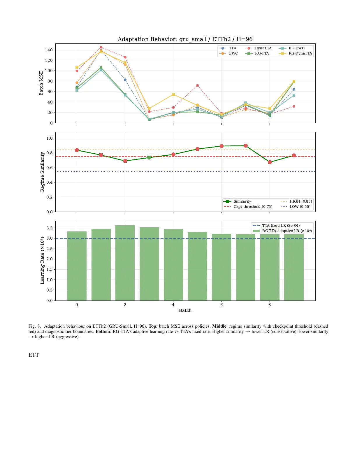
1 RG-TT A: Re gime-Guided Meta-Control for T est-T ime Adaptation in Streaming T ime Series Indar Kumar , Akanksha Tiw ari, Sai Krishna Jasti, and Ankit Hemant Lade Abstract —T est-time adaptation (TT A) enables neural f orecasters to adapt to distribution shifts in str eaming time series, but existing methods apply the same adaptation intensity regardless of the nature of the shift. W e propose Regime-Guided T est- Time Adaptation (RG-TT A), a meta-controller that continuously modulates adaptation intensity based on distributional similarity to pr eviously-seen r egimes. Using an ensemble of Kolmogoro v– Smirnov , W asserstein-1, feature-distance, and variance-ratio metrics, RG-TT A computes a similarity score for each incoming batch and uses it to (i) smoothly scale the learning rate—more aggressi ve f or novel distributions, conservati ve for familiar ones— and (ii) control gradient eff ort via loss-driven early stopping rather than fixed budgets, allowing the system to allocate exactly the effort each batch requires. As a supplementary mechanism, RG-TT A gates checkpoint reuse from a regime memory , loading stored specialist models only when they demonstrably outperf orm the current model (loss improv ement ≥ 30%). RG-TT A is model-agnostic and strategy-composable : it wraps any for ecaster exposing train/predict/save/load inter - faces and enhances any gradient-based TT A method. W e demonstrate three compositions—RG-TT A, RG-EWC, and RG- DynaTT A—and ev aluate 6 update policies (3 baselines + 3 regime- guided variants) across 4 compact architectur es (GRU , iT rans- former , P atchTST , DLinear), 14 datasets (6 real-world multiv ariate benchmarks + 8 synthetic regime scenarios), and 4 for ecast horizons (96, 192, 336, 720) under a streaming evaluation protocol with 3 random seeds (672 experiments total). Regime-guided policies achieve the lowest MSE in 156 of 224 seed-av eraged experiments (69.6%), with RG-EWC winning 30.4% and RG-TT A winning 29.0%. Overall, RG-TT A reduces MSE by 5.7% vs TT A while running 5.5% faster; RG-EWC reduces MSE by 14.1% vs standalone EWC. Against full retraining (672 additional experiments, 3 architectures excluding DLinear), RG policies achieve a median 27% MSE reduction while running 15–30 × faster , winning 71% of seed-averaged configurations. The regime-guidance layer composes naturally with existing TT A methods, impro ving accuracy without modifying the underlying for ecaster . I . I N T RO D U C T I O N T ime series forecasting in production is inherently incremen- tal: data arriv es in batches, and the system must decide how to update its model [1], [2]. T est-time adaptation (TT A) [3] has emerged as a practical approach, applying a fixed number of gradient steps to each incoming batch. Recent work has improv ed upon fixed TT A: T AF AS [4] freezes the source model and learns calibration modules (GCMs) that adapt predictions, while DynaTT A [5] dynamically adjusts the learning rate based on prediction-error z-scores and embedding drift. Code and data are available at https://github.com/IndarKarhana/RGTT A- Regime- Guided- T est- Time- Adaptation. I. Kumar, A. Tiwari, S. K. Jasti, and A. H. Lade are independent researchers (e-mail: indarkarhana@gmail.com, akankshat2803@gmail.com, jsaikrishna379@gmail.com, ankitlade12@gmail.com). Howe v er , DynaTT A (and similar reactiv e methods) react to current performance signals without asking the pr oactive question: has the system seen this distribution before? If a previously-encountered regime recurs, the highest-accuracy strategy is to load the checkpoint trained for that regime— not to re-adapt from a potentially stale model, which wastes gradient budget re-learning patterns that were already captured. W e propose Regime-Guided T est-Time Adaptation (RG- TT A) , a meta-controller that adds this proacti ve layer . For each incoming batch, RG-TT A: 1) Extracts a 5-dimensional distributional feature v ector (mean, std, ske wness, excess kurtosis, lag-1 autocorre- lation). 2) Computes similarity to all stored re gime checkpoints using an ensemble of K olmogoro v–Smirnov , W asserstein- 1, feature-distance, and v ariance-ratio metrics. 3) Uses the similarity score to continuously modulate adap- tation: • Learning rate scales smoothly with novelty: α = α base · (1 + γ · (1 − sim )) , where γ = 0 . 67 . • Checkpoint reuse is loss-gated: stored checkpoints are loaded only when sim ≥ 0 . 75 and the checkpoint’ s loss is < 0 . 70 × the current model’ s loss ( ≥ 30% improv ement). • Step count is determined by loss-driv en early stopping (patience = 3 , ϵ = 0 . 005 ), up to a maximum of 25 steps. RG-TT A is model-a gnostic : it requires only train() , predict() , and save/load_weights() interfaces and can wrap any forecaster . It is also strate gy-composable : the regime-guidance layer can enhance any gradient-based adapta- tion method (TT A, EWC, DynaTT A), yielding RG-TT A, RG- EWC, and RG-DynaTT A v ariants. Our contributions are: 1) A continuous regime-guided adaptation policy that modulates learning rate, step budget, and checkpoint reuse based on distributional similarity , using an ensemble of four complementary similarity metrics and loss-driven early stopping. 2) A composable meta-controller architecture where regime-guidance wraps gradient-based adaptation meth- ods, demonstrated with three compositions (RG-TT A, RG-EWC, RG-DynaTT A) tar geting dif ferent accuracy– robustness trade-offs. 3) A comprehensive benchmark spanning 6 update policies (plus full retraining), 4 compact model architectures, 14 datasets, 4 forecast horizons, and 3 random seeds (672 experiments, plus 672 retrain-baseline experiments)—to 2 our knowledge, the most e xtensiv e controlled comparison of TT A strategies for streaming time series forecasting. I I . R E L A T E D W O R K a) T est-time adaptation for time series.: TT A [3] adapts a pre-trained model to test-time distribution shifts by running additional gradient steps. In the time series setting, T AF AS [4] proposes freezing the source model and training lightweight Gated Calibration Modules (GCMs) that adjust inputs and outputs to the current distribution, using only pseudo-labels from the model’ s o wn predictions (POGT loss). DynaTT A [5] extends T AF AS with a dynamic learning rate computed via a sigmoid transformation of three shift metrics: prediction-error z-score, and distances to recent (R T AB) and representativ e (RDB) embedding b uffers. Both methods are reactive —the y adjust to the current batch based on real-time error and drift signals. RG-TT A adds a pr oactive layer: it identifies whether the current distribution has been seen before and adapts its strategy accordingly . RG-TT A composes naturally with DynaTT A (RG- DynaTT A); we demonstrate this as a two-lev el controller . Reimplementation note. DynaTT A ’ s of ficial codebase ( shivam-grover/DynaTTA ) implements the dynamic learning rate within the T AF AS framework—tightly coupled with GCM calibration modules, the POGT pseudo-label loss, and a sliding-windo w ev aluation harness. No standalone library or modular API is provided. Because our study requires a model-agnostic streaming ev aluation pipeline that applies each update policy to the same frozen-backbone base model, we reimplemented DynaTT A ’ s Algorithm 1 (dynamic LR via sigmoid of prediction-error z-score, R T AB/RDB embedding distances, and EMA smoothing) from the published descrip- tion. Our implementation reproduces the published formula exactly with the published hyperparameters ( α min = 10 − 4 , α max = 10 − 3 , κ = 1 . 0 , η = 0 . 1 ). W e validate on the same architectures targeted by DynaTT A (iTransformer , P atchTST). W e note that DynaTT A ’ s EMA coefficient ( η = 0 . 1 ) requires ∼ 22 gradient steps to con ver ge, a design choice suited to the 500-window sliding-window protocol used in its original e valuation. Under our streaming protocol (10 batches per run), the EMA does not con ver ge within the av ailable budget, leaving the dynamic LR below TT A ’ s fixed rate for the first 5–6 batches. This is a pr otocol-level mismatch , not an implementation error (see Limitations §IX, item 7). T AF AS [4] is a strong baseline at short horizons (H ≤ 192) where its frozen-source GCM calibration e xcels, but its performance collapses at longer horizons (H=336/720, + 100– 400% vs TT A in our experiments)—a consequence of its design for sliding-window ev aluation. Because our study spans H ∈ {96,192,336,720}, we include T AF AS as a reference policy but exclude it from the primary 6-policy comparison. b) Continual learning and catastr ophic for getting.: Continual learning [6], [7] addresses the problem of updating a model on sequential tasks without forgetting old knowledge. EWC [8] penalises changes to parameters important for previous tasks via the diagonal Fisher Information Matrix. Synaptic Intelligence [9] tracks parameter importance online. Experience replay [10] stores and re-uses past data samples. Progressiv e networks [11] add capacity for new tasks. Our approach is complementary: rather than regularising a single model, RG-TT A maintains a library of chec kpoints indexed by distributional features and selects the appropriate one. When combined with EWC (RG-EWC), the regime-guided adaptation operates under EWC regularisation ( λ = 400 ), preventing catastrophic forgetting while benefiting from checkpoint reuse and similarity-modulated learning rates. c) Concept drift and r e gime switching.: Concept drift de- tection [12]–[14] identifies that a distribution change occurred. Our approach extends this by detecting not just change b ut r ecurr ence —whether the new distribution matches a previously- seen re gime. Hamilton’ s Markov-switching model [15] uses latent states for regime transitions but assumes a specific generativ e process. RG-TT A makes no parametric assump- tion: “regime” is defined operationally by a 5-dimensional distributional feature vector , and matching uses non-parametric statistical tests. d) T ime series forecasting arc hitectur es.: Recent neural forecasters—Informer [16], Autoformer [17], iT ransformer [18], PatchTST [19], DLinear [20]—adv ance accuracy but do not address the when-to-adapt question. W e ev aluate RG- TT A across four compact model architectures spanning three model families—recurrent (GR U [21]), attention-based (iTrans- former , PatchTST), and linear (DLinear)—to validate model- agnosticism. Notably , iT ransformer and PatchTST are the same modern Transformer architectures tar geted by DynaTT A [5]. I I I . M E T H O D Figure 1 provides an end-to-end overvie w of the RG- TT A pipeline; its main components—distributional similarity (§ III-B ), continuous regime-guided adaptation (§ III-C ), and checkpoint management (§ III-F )—are detailed in the subsec- tions below . A. Pr oblem Setup Data arriv es as a stream of batches B 1 , B 2 , . . . (batch size 750). A base forecaster f θ can be trained, saved, and loaded. At each step t , batch B t arriv es; the system produces a forecast ˆ y t +1: t + H for horizon H ∈ { 96 , 192 , 336 , 720 } and optionally updates θ . All 6 compared policies share the same f θ architecture, the same data splits, and the same random seeds; only the update rule differs. B. Distributional Similarity Metric For each batch, RG-TT A extracts a 5-dimensional distribu- tional feature vector: r =  µ, σ, γ 1 , κ − 3 , r 1  , (1) where µ is the mean, σ the standard deviation, γ 1 the ske wness, κ − 3 the excess kurtosis, and r 1 the lag-1 autocorrelation. These features are computed from the most recent 3 × season_length samples of the target series and capture the distribution’ s location, scale, shape, tail behaviour , and temporal structure in O ( n ) time. The deliberate simplicity of this feature vector is a design choice, not a limitation: it is cheap to compute (adding 3 New Batch B t Extract F e a t u r e s r Compute Similarity Loss-Gated Ckpt Load Smooth LR Modulation Adapt Head (early stop) Save to Memory F orecast y t + H C h e c k p o i n t M e m o r y ( 5 s l o t s , F I F O ) s i m 0 . 7 5 ? c k p t < 0 . 7 c u r r KS + W asserstein + F eature + V ariance = b a s e ( 1 + ( 1 s i m ) ) Frozen backbone max 25, patience 3 query store ckpt RG - T T A: Regime-Guided T est- Time Adaptation Pipeline Fig. 1. RG-TT A system ov erview . For each incoming batch B t , the system extracts a distributional feature v ector r (Eq. 1) and computes a similarity score sim against stored regimes using a four-metric ensemble (Eq. 6). If a high-similarity checkpoint passes the loss gate ( ℓ ckpt < 0 . 70 ℓ curr , Eq. 8), it replaces the current model. The learning rate is smoothly modulated by similarity (Eq. 7), and the output head is adapted with loss-driven early stopping (max 25 steps, patience 3). The adapted checkpoint and its regime features are stored in the memory M (dashed box; 5 slots, FIFO eviction) for future reuse. See Algorithm 1 for pseudocode. < 0.1% latency), fully interpretable, and—as the 69.6% win rate across 14 div erse datasets confirms— sufficient for effectiv e regime discrimination. Richer representations (e.g., learned embeddings or spectral features) could capture more complex regime structures, but at the cost of additional parameters, training overhead, and opacity . Similarity between a query batch q and a stored regime s is computed as a weighted ensemble of four complementary metrics: a) K olmogor ov–Smirnov similarity .: Based on the tw o- sample KS statistic [22] on the raw values: sim KS = 1 − D n , D n = sup x | F q ( x ) − F s ( x ) | . (2) b) W asserstein-1 similarity .: Normalised earth-mov er’ s distance [23]: sim W = 1 1 + W 1 ( q raw , s raw ) / max( ptp ( q raw ) , ptp ( s raw ) , ϵ ) . (3) c) F eatur e-distance similarity .: Normalised Euclidean distance in feature space: sim feat = 1 1 + ∥ q − s ∥ 2 /  ( ∥ q ∥ 2 + ∥ s ∥ 2 ) / 2 + ϵ  . (4) d) V ariance-ratio similarity .: Captures v olatility regime shifts: sim var = min( σ q , σ s ) max( σ q , σ s ) + ϵ . (5) e) W eighted ensemble .: sim ( q , s ) = 0 . 3 · sim KS + 0 . 3 · sim W + 0 . 2 · sim feat + 0 . 2 · sim var . (6) The statistical tests (KS, W asserstein) use the full empirical distribution and recei ve higher weight (0.3 each) because they are non-parametric and distribution-free, capturing arbitrary shape differences that scalar features may miss. The feature- distance and variance-ratio metrics receiv e lower weight (0.2 each) as they provide complementary but narrower information (higher-order moments and volatility regime shifts, respec- ti vely). W e chose these weights a priori based on the principle of giving distrib utional tests priority ov er scalar summaries, and did not tune them on validation data. The ablation in T able X confirms the ensemble is robust: it outperforms ev ery single-metric variant, and the 1.8% gap to the best single component (W asserstein) suggests the ensemble’ s v alue lies in complementary coverage rather than precise weight selection. C. Continuous Re gime-Guided Adaptation Rather than discretising similarity into fixed tiers with predetermined step counts, RG-TT A uses the similarity score as a continuous control signal for three adaptation dimensions: a) Smooth learning rate modulation.: The learning rate scales smoothly with distrib utional novelty: α = α base ·  1 + γ · (1 − sim )  , (7) where α base = 3 × 10 − 4 (matching TT A ’ s default) and γ = 0 . 67 is the similarity scale factor . At sim = 1 . 0 (perfect match), α = α base (conserv ativ e); at sim = 0 . 5 (moderate novelty), α ≈ 1 . 34 × α base ; at sim = 0 . 0 (complete novelty), α ≈ 1 . 67 × α base (most aggressiv e). This avoids the sensiti vity of hard thresholds and provides a natural scaling: f amiliar distrib utions need less correction. b) Loss-gated chec kpoint reuse .: When the best-matching stored regime has sim ≥ 0 . 75 , RG-TT A e v aluates the stored checkpoint by running a forward pass on the current batch. The checkpoint is loaded only if its loss satisfies: ℓ ckpt < 0 . 70 · ℓ curr , (8) 4 Algorithm 1 RG-TT A: Regime-Guided T est-T ime Adaptation Require: Batch B t , checkpoint memory M , base LR α base , scale γ , gate g 1: q ← features ( B t ) {Eq. 1: 5-D distrib ution vector} 2: ( sim ∗ , θ ∗ ckpt ) ← max s ∈M sim ( q , s ) {Eq. 6: 4-metric ensemble} 3: ℓ curr ← L ( f θ ( X t ) , y t ) {Current model loss on ne w batch} 4: if sim ∗ ≥ 0 . 75 then 5: ℓ ckpt ← L ( f θ ∗ ckpt ( X t ) , y t ) 6: if ℓ ckpt < g · ℓ curr then 7: θ ← θ ∗ ckpt ; ℓ curr ← ℓ ckpt 8: end if 9: end if 10: α ← α base · (1 + γ · (1 − sim ∗ )) {Eq. 7: smooth LR scaling} 11: patience ← 0 12: for k = 1 to K max do 13: ˆ y = f θ head ( X t ) {Backbone frozen; only output head updated} 14: L = SmoothL1 ( ˆ y , y t ) [24] {+ optional EWC/DynaTT A terms} 15: θ head ← θ head − α ∇ θ head L 16: if k ≥ K min and ( ℓ k − 1 − ℓ k ) / | ℓ k − 1 | < ϵ then 17: patience ← patience +1 18: if patience ≥ 3 then 19: break {Early stop: loss con v erged} 20: end if 21: else 22: patience ← 0 23: end if 24: end for 25: M [ q ] ← ( θ , metadata ) {Store checkpoint for future reuse} 26: retur n ˆ y t +1: t + H i.e., the checkpoint must achiev e at least a 30% loss im- prov ement over the current model. This strict gate prev ents rev erting to stale checkpoints on slo wly-drifting data, where the continuously-adapted live model may already outperform historical specialists. c) Loss-driven early stopping.: Rather than a fix ed step budget, RG-TT A runs up to K max = 25 gradient steps with early stopping: if the relati ve loss improvement falls below ϵ = 0 . 005 for 3 consecutiv e steps (after a minimum of K min = 5 steps), adaptation halts. This allows RG-TT A to naturally allocate more effort to difficult batches (nov el distributions requiring full budget) and less to easy ones (familiar distrib utions con ver ging quickly). In practice, RG-TT A av erages 18.5 steps per batch (median 24), compared to TT A ’ s fixed 20. While 49% of batches use the full 25-step budget (nov el regimes), 12% conv erge in ≤ 8 steps (familiar regimes), producing the net 5.5% wall-clock speedup (T able VIII). Algorithm 1 gives the pseudocode. D. RG-EWC: Re gime-Guided EWC RG-EWC adds EWC regularisation [8] to the RG-TT A framew ork. The total loss becomes: L total = L task + λ 2 X i F i ( θ i − θ ∗ i ) 2 , (9) where F i is the diagonal Fisher Information (estimated from 200 samples, clamped to [0 , 10 4 ] ), θ ∗ is the anchor (updated after each batch), and λ = 400 . When a checkpoint is loaded via the loss gate, the EWC anchor θ ∗ is reset to the loaded parameters to prevent penalising movement away from the pre- load state. Fisher is maintained online via exponential moving av erage: F ( t ) = 0 . 5 · F ( t − 1) + 0 . 5 · ˆ F new . The ke y advantage of RG-EWC ov er standalone EWC is tar geted adaptation : EWC prevents catastrophic forgetting while the regime-guided learning rate and checkpoint reuse improv e the starting point and con v ergence trajectory . In our benchmark, RG-EWC reduces MSE by 14.1% vs standalone EWC and wins 75.4% of head-to-head comparisons (169/224 experiments). E. RG-DynaTT A: T wo-Level Contr oller RG-DynaTT A combines pr oactive regime detection (RG- TT A) with r eactive shift-magnitude sensing (DynaTT A [5]). Instead of the similarity-based smooth LR (Eq. 7), DynaTT A ’ s sigmoid formula computes the actual LR based on three shift metrics (prediction-error z-score, R T AB/RDB embedding dis- tances). This creates a two-lev el controller: RG-TT A pro vides checkpoint reuse and loss-driv en early stopping; DynaTT A provides the continuous LR within [ α min , α max ] based on current error signals. F . Checkpoint Management Each checkpoint stores: (i) complete model weights, (ii) the 5-D regime feature vector , (iii) ra w batch values for KS/W asserstein computation, and (iv) metadata including the fitted preprocessor (scaler) state. Co-saving the preprocessor is critical: loading a checkpoint restores both the model and the normalisation parameters used during its training. The memory is capped at 5 entries with FIFO e viction. G. F r ozen Bac kbone Adaptation All gradient-based adaptation policies (TT A, EWC, Dy- naTT A, RG-TT A, RG-EWC, RG-DynaTT A) freeze the model backbone during test-time adaptation and update only the output projection layer . For GRU-Small ( 71 K total parameters), this leav es ∼ 10 K trainable ( ∼ 15% ); for iTransformer ( 123 K total), ∼ 6 K trainable ( ∼ 5% ); for PatchTST ( 192 K total), ∼ 68 K in the flatten-to-forecast head ( ∼ 35% ); for DLinear ( 37 K at H=96), ∼ 19 K in the trend/seasonal linear layers ( ∼ 50% ). This mirrors the linear-probing paradigm in vision TT A and provides implicit regularisation: the learned temporal representations in the backbone are preserved, and only the mapping from hidden states to forecast v alues is recalibrated. Howe v er , the effecti veness of frozen-backbone TT A is ar chitectur e-dependent : it works well for models where the 5 backbone learns reusable temporal representations (GR U, DLinear), but is less effecti ve for attention-based architectures (iT ransformer , PatchTST) where the attention patterns them- selves need to shift to accommodate ne w distributions. This is a shared limitation across all gradient-based TT A policies, not specific to RG-TT A. I V . T H E O R E T I C A L A N A L Y S I S W e provide formal analysis of RG-TT A ’ s three design pillars: frozen-backbone adaptation (§ IV -B ), similarity-guided initial- isation (§ IV -A ), and the ensemble similarity metric (§ IV -C ). T ogether , these results establish that RG-TT A ’ s mechanisms are principled—not merely heuristic—and yield quantitative conditions under which re gime-guidance prov ably improv es upon fixed-strategy TT A. W e note that the analysis assumes strong conv exity and smoothness of the output-head loss landscape—reasonable for the single linear layer that constitutes the trainable head, but an idealisation relati ve to the Adam optimiser and finite-batch noise used in practice. The theoretical results should therefore be read as design rationale and dir ectional guarantees , not tight performance predictions; the empirical results in §VI provide the definiti ve ev aluation. A. Adaptation Err or Decomposition W e analyse per-batch adaptation error under the frozen- backbone constraint. Let f θ = h ϕ ◦ g ψ where g ψ : R L × d in → R d h is the frozen backbone and h ϕ : R d h → R H is the trainable output head with d head parameters. Definition 1 (Batch-optimal parameters) . F or batch B t drawn fr om distribution P t , define ϕ ∗ t = arg min ϕ E ( x,y ) ∼ P t [ ℓ ( h ϕ ( g ψ ( x )) , y )] as the head parameters minimising the population loss on the current r e gime. Theorem 1 (Adaptation error bound) . Assume the per-batch loss L ( ϕ ) = E B t [ ℓ ( h ϕ ( g ψ ( x )) , y )] is µ -str ongly con vex and L -smooth in ϕ with condition number κ = L/µ . After K gradient descent steps with learning rate α ∈ (0 , 2 /L ) fr om initialisation ϕ 0 : ∥ ϕ K − ϕ ∗ t ∥ 2 ≤ ρ 2 K ∥ ϕ 0 − ϕ ∗ t ∥ 2 , wher e ρ = 1 − 2 µα 1 + µα < 1 . (10) The expected per-batc h MSE decomposes as: E [ ℓ ( ϕ K )] = σ 2 t |{z} irr educible + ρ 2 K ∥ ϕ 0 − ϕ ∗ t ∥ 2 H | {z } adaptation residual , (11) wher e σ 2 t = E P t [ ∥ y − h ϕ ∗ t ( g ψ ( x )) ∥ 2 ] is the irr educible noise under the fr ozen bac kbone and ∥ · ∥ H is the Hessian-weighted norm. Pr oof. Under µ -strong con v exity and L -smoothness, gradient de- scent with α ≤ 2 / ( µ + L ) satisfies the standard contraction [25]: ∥ ϕ k +1 − ϕ ∗ t ∥ 2 ≤ ρ 2 ∥ ϕ k − ϕ ∗ t ∥ 2 with ρ = ( L − µ ) / ( L + µ ) = ( κ − 1) / ( κ + 1) = 1 − 2 µα/ (1 + µα ) at the optimal step size α ∗ = 2 / ( µ + L ) . Iterating K times yields Eq. 10. The MSE decomposition follo ws from expanding E [ ℓ ( ϕ K )] around ϕ ∗ t and using the second-order T aylor approximation of the loss. ■ a) Impact of chec kpoint loading.: When RG-TT A loads a checkpoint ϕ ckpt trained on a previous occurrence of a regime with similarity s to the current batch, the initialisation changes from ϕ 0 (current model) to ϕ ckpt . If the stored checkpoint was optimal for a regime at distrib utional distance proportional to (1 − s ) , the initialisation error satisfies: ∥ ϕ ckpt − ϕ ∗ t ∥ 2 ≤ (1 − s ) 2 · D 2 max , (12) where D max = sup t ∥ ϕ 0 − ϕ ∗ t ∥ is the worst-case distance. Substituting into Eq. 11: E [ ℓ RG ( ϕ K )] ≤ σ 2 t + ρ 2 K (1 − s ) 2 D 2 max . (13) This reveals three mechanisms for reducing per -batch error: (i) more gradient steps K (the TT A approach), (ii) better initialisation via checkpoint loading, reducing (1 − s ) 2 (the RG- TT A approach), and (iii) both simultaneously . The improv ement factor (1 − s ) 2 quantifies the benefit: at s = 0 . 85 (HIGH similarity), the initialisation error reduces by 97 . 75% ; at s = 0 . 55 (MID), by 79 . 75% . Corollary 1 (Step savings from checkpoint reuse) . T o achieve adaptation r esidual ≤ ϵ , TT A r equir es K TT A ≥ log( D 2 max /ϵ ) 2 | log ρ | steps, while RG-TT A with chec kpoint similarity s r equir es K RG ≥ log  (1 − s ) 2 D 2 max /ϵ  2 | log ρ | steps. The per-batch savings ar e: ∆ K = K TT A − K RG = − log(1 − s ) | log ρ | . (14) F or s = 0 . 85 and ρ = 0 . 95 : ∆ K ≈ 37 steps—exceeding the budg et K max = 25 , meaning the chec kpoint is alr eady near- optimal and early stopping activates within K min = 5 steps. F or s = 0 . 55 : ∆ K ≈ 16 steps. This corollary provides the theoretical basis for RG-TT A ’ s computational efficiency (T able VIII): by starting closer to the optimum, fewer gradient steps are needed, and the loss-driv en early stopping mechanism (§ III-C ) naturally terminates when the residual is small. B. Generalisation Bound under F r ozen Bac kbone The frozen-backbone constraint restricts the ef fecti ve h y- pothesis class, pro viding implicit regularisation. W e formalise this via Rademacher comple xity . Theorem 2 (Generalisation bound for frozen-backbone adap- tation) . Let F full = { x 7→ h ϕ ( g ψ ( x )) : ϕ ∈ Φ , ψ ∈ Ψ } be the full model class and F fr ozen = { x 7→ h ϕ ( g ψ ∗ ( x )) : ϕ ∈ Φ } the fr ozen-bac kbone class with fixed ψ ∗ . Assume the output head is linear: h ϕ ( z ) = W z + b with ∥ W ∥ F ≤ B W and ∥ g ψ ∗ ( x ) ∥ ≤ C g for all x ∈ X . Then for n i.i.d. samples fr om P t with bounded loss ℓ ∈ [0 , c ] , the empirical Rademacher complexity of ℓ ◦ F fr ozen satisfies: ˆ R n ( ℓ ◦ F fr ozen ) ≤ c ℓ B W C g √ n , (15) wher e c ℓ is the Lipschitz constant of ℓ . W ith pr obability at least 1 − δ over the dr aw of n samples: R ( ˆ f ) ≤ ˆ R n ( ˆ f ) + 2 c ℓ B W C g √ n + 3 r ln(2 /δ ) 2 n , (16) 6 wher e R ( ˆ f ) = E P t [ ℓ ( ˆ f ( x ) , y )] is the population risk and ˆ R n ( ˆ f ) is the empirical risk. Pr oof. The proof follows the standard Rademacher complexity argument [26]. Since g ψ ∗ is fixed, the hypothesis class F frozen is a linear class in the representation space g ψ ∗ ( X ) . By T alagrand’ s contraction lemma [27] and the Rademacher complexity of linear classes with bounded Frobenius norm [26], we obtain Eq. 15. The generalisation bound Eq. 16 follo ws from McDiarmid’ s inequality [28]. ■ a) Comparison with full-model adaptation.: For the full class F full with d total free parameters, the covering-number argument gives ˆ R n ( ℓ ◦ F full ) = O  p d total log n/n  . The ratio of complexities is: ˆ R n ( F frozen ) ˆ R n ( F full ) ∝ s d head d total . (17) For GR U-Small ( d head ≈ 10 K, d total ≈ 71 K), this ratio is ≈ 0 . 38 —a ∼ 2 . 6 × tighter generalisation bound. For iTransformer ( d head ≈ 6 K, d total ≈ 123 K), the ratio is ≈ 0 . 22 ( ∼ 4 . 5 × tighter). This formalises the empirical observation that frozen-backbone adaptation outperforms full-model fine-tuning within the limited step budgets ( K ≤ 25 ) of test-time adaptation: the restricted hypothesis class trades representational capacity for statistical efficienc y . C. Consistency of the Ensemble Similarity Metric Proposition 1 (Metric properties) . The ensemble similarity sim ( · , · ) defined in Eq. 6 satisfies the following pr operties: 1) Boundedness: sim ( q , s ) ∈ [0 , 1] for all batc hes q , s . 2) Self-similarity: sim ( q , q ) = 1 . 3) Symmetry: sim ( q , s ) = sim ( s , q ) . 4) Statistical consistency: If ˆ P n d − → P and ˆ Q m d − → Q as n, m → ∞ , then sim ( ˆ P n , ˆ Q m ) → sim ( P , Q ) . 5) Discriminative power: F or continuous distributions, sim ( P , Q ) = 1 implies P = Q . Pr oof. Properties 1–3 are immediate from the definitions of the component metrics: D n ∈ [0 , 1] (KS statistic), W 1 ≥ 0 (W asserstein-1), and the normalised forms (Eqs. 3–5) are each bounded in [0 , 1] ; any con vex combination inherits these properties. Property 4 follows from the Glivenk o–Cantelli the- orem [29] for the KS component ( sup x | F n ( x ) − F ( x ) | a.s. − − → 0 ) and the con vergence of the empirical W asserstein-1 distance on the real line [30]. For property 5: sim KS = 1 implies D n = 0 , i.e., F P = F Q , which uniquely determines P = Q for continuous distrib utions by the one-to-one correspondence between CDFs and distrib utions. ■ a) Complementary sensitivity .: The four components detect different shift types: KS is most sensitive to shape changes (symmetry , modality), W asserstein-1 to location-scale shifts, the feature-distance metric to higher-order moment changes (kurtosis, autocorrelation), and the variance ratio to pure volatility shifts. The ensemble achiev es strictly better robustness than any single metric (T able X), improving over the best single component by 1.8% MSE and o ver the w orst (feature-only , our v0 design) by 8.3%. D. Optimal Checkpoint Loading Condition Proposition 2 (Sufficient condition for beneficial checkpoint loading) . Under the conditions of Theor em 1, let ℓ K curr and ℓ K ckpt denote the post-adaptation losses after K gradient steps fr om ϕ curr and ϕ ckpt r espectively . Loading the c heckpoint is beneficial ( ℓ K ckpt ≤ ℓ K curr ) whenever: ∥ ϕ ckpt − ϕ ∗ t ∥ ≤ ∥ ϕ curr − ϕ ∗ t ∥ . (18) The loss gate (Eq. 8) with g = 0 . 70 is a sufficient condition for Eq. 18: under µ -str ong conve xity , ℓ ( ϕ ckpt ) < g · ℓ ( ϕ curr ) implies ∥ ϕ ckpt − ϕ ∗ t ∥ < √ g · ∥ ϕ curr − ϕ ∗ t ∥ ≈ 0 . 84 ∥ ϕ curr − ϕ ∗ t ∥ . Pr oof. Under µ -strong con ve xity: µ 2 ∥ ϕ − ϕ ∗ t ∥ 2 ≤ L ( ϕ ) − L ( ϕ ∗ t ) . If ℓ ( ϕ ckpt ) < g · ℓ ( ϕ curr ) , then L ( ϕ ckpt ) − σ 2 t < g ( L ( ϕ curr ) − σ 2 t ) + ( g − 1) σ 2 t ≤ g ( L ( ϕ curr ) − σ 2 t ) (since g < 1 ). Applying the strong con ve xity lower bound: µ 2 ∥ ϕ ckpt − ϕ ∗ t ∥ 2 ≤ g · L 2 ∥ ϕ curr − ϕ ∗ t ∥ 2 , gi ving ∥ ϕ ckpt − ϕ ∗ t ∥ ≤ √ g κ ∥ ϕ curr − ϕ ∗ t ∥ . For well-conditioned losses ( κ ≈ 1 ), √ g ≈ 0 . 84 , confirming the checkpoint is closer . ■ This formalises the dual-gate design: the similarity threshold ( s ≥ 0 . 75 ) serv es as a cheap filter that identifies regime- compatible checkpoints in O ( M ) time, while the loss g ate ( ℓ ckpt < 0 . 70 · ℓ curr ) serves as a precise criterion that guarantees parameter-space proximity via an O ( | θ | ) forward pass. The 30% improv ement threshold is deliberately conserv ativ e—it av oids loading marginally-better checkpoints that may have ov erfit to a previous regime’ s idiosyncrasies. V . E X P E R I M E N T S A. Datasets W e ev aluate on 14 datasets spanning two categories: a) Real-world benchmarks (6).: ETTh1, ETTh2 (hourly , 17,420 rows), ETTm1, ETTm2 (15-minute, 69,680 ro ws) [16], W eather (52,696 rows, 21 features), and Exchange (7,588 rows, 8 currencies). These are standard benchmarks used by DynaTT A [5] and T AF AS [4]; we overlap on 6 of their 7 datasets (missing only Illness). b) Synthetic r e gime scenarios (8).: Purpose-built series that isolate specific adaptation challenges: • synth_stable : Stationary baseline (no regime changes). • synth_trend_break : Single abrupt trend re versal. • synth_slow_drift : Gradual parameter ev olution. • synth_fast_switch : Rapid alternation between 2 regimes. • synth_recurring : 3 re gimes that cycle periodically . • synth_volatility : Smooth volatility regime transi- tions. • synth_shock_recovery : Sudden shock followed by recov ery . • synth_multi_regime : 4+ regimes with comple x transitions. B. Model Arc hitectur es T o validate model-agnosticism, we test 4 compact model architectures ( 37K–192K parameters ) spanning recurrent, attention-based, and linear families. 7 T ABLE I M O DE L A R C H IT E C T UR E S U S ED I N E X P ER I M EN T S . A L L P O L I CI E S U S E T H E S A ME M O DE L P E R E X P ER I M E NT . Ke y Architecture Parameters Family gru_small 2-layer GRU + MLP head ∼ 71 K Recurrent itransformer iT ransformer [18] ∼ 123 K Attention patchtst PatchTST [19] ∼ 192 K Attention dlinear DLinear [20] ∼ 37 K– 1 . 2 M Linear C. Update P olicies (6 primary) All 6 policies receive identical data, use the same base model per experiment, and share the same random seed. Only the update strategy differs. a) P olicy ablation logic.: The 6 policies form a controlled hierarchy: • RG-TT A vs TT A : Does regime-guidance improv e over fixed adaptation? • RG-EWC vs EWC : Does regime-guided EWC beat always-on EWC? • RG-DynaTT A vs DynaTT A : Does adding regime- awareness improve DynaTT A? Each RG-variant differs from its baseline only in adding the re gime-guidance layer (similarity-scaled LR, checkpoint reuse, early stopping). This isolates the contribution of regime- awareness. b) Full retr ain baseline.: W e additionally benchmark full retraining from scratch on all accumulated data at each batch, reported separately due to its 15–30 × higher computational cost (§VI-J). D. Evaluation Pr otocol a) Str eaming protocol.: Initial training on 720 rows, then sequential processing of up to 10 batches of 750 rows each. Each policy receives the same batches in order , updates its model, and predicts the next H values. For hourly data, the initial 720 rows correspond to ∼ 30 days; each batch represents ∼ 31 days; the full sequence spans ∼ 11 months of deployment. b) Why str eaming evaluation.: W e ev aluate under the streaming protocol exclusi vely because it reflects how fore- casting systems operate in production: data arri ves in discrete batches (e.g., daily or weekly), the system must update and produce forecasts before the next batch arrives, and adaptation decisions accumulate over time. This is the standard deployment model for ener gy forecasting (ETT datasets), weather services, and financial trading desks. The sliding-window protocol used by DynaTT A [5] and T AF AS [4]—where each windo w receiv es exactly one gradient step—is a useful of fline e valuation tool but does not reflect how practitioners deplo y TT A: no production system retrains from a sliding window of 500 ov erlapping samples. Furthermore, the sliding-window protocol structurally neutralises RG-TT A ’ s key contributions: (i) checkpoint reuse becomes counterproductive because the model changes by only one gradient step between windows, (ii) early stopping is irrelev ant when the b udget is always 1 step, and (iii) regime memory cannot b uild because consecuti ve windows ov erlap by > 99%. Our streaming protocol preserves the full decision space— how many steps , at what learning rate , and fr om which starting point —allo wing all policies to exercise their complete strategies. E. Metrics W e report MSE, MAE, RMSE, sMAPE, wMAPE (weighted MAPE with exponential recency weights), and direction accuracy . All metrics are averaged across batches within each experiment, then across 3 random seeds. Statistical significance is assessed via W ilcoxon signed-rank tests [31] with Bonferroni correction for multiple comparisons. Overall policy ranking uses the Friedman test [32] with Nemenyi post-hoc, follo wing [33]. 8 T ABLE II T H E 6 U P DA T E P O L IC I E S . P O L I CI E S 1 – 3 A R E BA S E L IN E S ; 4 – 6 A R E O U R C O N TR I B UT I O N S . “ R E GI M E M E M . ” I N D IC ATE S W H ET H E R T H E P O L I CY M A I NTA IN S A C H EC K P O IN T L I B RA RY . # Policy Steps K LR Regime mem. Ke y mechanism 1 TT A 20 (fixed) 3 × 10 − 4 No Fixed-step gradient adaptation 2 EWC 15 (fixed) 3 × 10 − 4 No Fisher-penalised adaptation 3 DynaTT A 20 (fixed) Dynamic No Sigmoid LR from shift metrics 4 RG-TT A ≤ 25 (early stop) Sim-scaled Y es Continuous regime-guided TT A 5 RG-EWC ≤ 25 (early stop) Sim-scaled Y es + EWC regularisation ( λ =400) 6 RG-DynaTT A ≤ 25 (early stop) DynaTT A+RG Y es + DynaTT A sigmoid LR V I . R E S U L T S W e present results from 672 experiments (6 policies × 4 models × 14 datasets × 4 horizons × 3 seeds), plus 672 retrain-baseline experiments compared in § VI-J . All tables report seed-averaged values (224 unique experiments). A. Overall W in Counts T able III reports how many of the 224 seed-averaged experiments each polic y wins (lo west MSE). B. P air-wise Regime-Guidance Effect T able IV isolates the ef fect of adding regime-guidance to each baseline by comparing matched pairs. RG-EWC shows the strongest regime-guidance benefit: − 14 . 1% MSE reduction with 75.4% win rate. For RG- DynaTT A, the av erage improv ement is near zero (skewed by synthetic outliers with extreme scale), but the median improv ement is − 3 . 8% and it wins 62.1% of experiments, indicating consistent benefit. All three improvements are statistically significant (W ilcoxon signed-rank, p < 0 . 007 , Bonferroni-corrected; T able IV). The regime-guidance layer improv es all three base methods—the composability claim holds empirically . Figure 2 visualises these pair-wise effects. C. MSE by Model Arc hitectur e T able V reports a verage MSE across all 14 datasets and 4 horizons, broken down by model architecture. RG-TT A and RG-EWC are best on GR U-Small ( − 8 . 8% and − 9 . 1% vs TT A) and iT ransformer ( − 8 . 9% and − 10 . 6% ). On P atchTST , policies cluster tightly (TT A edges RG-TT A by < 0 . 2% ). On DLinear , RG-DynaTT A wins ( − 2 . 6% vs DynaTT A). The adv antage is strongest on recurrent models where the frozen backbone preserves reusable temporal features. Figure 3 provides a visual comparison on real-world data. D. Statistical Ranking T o rigorously compare all 6 policies simultaneously , we apply the Friedman test [32], [33] across 224 seed-a veraged experiments. The null hypothesis that all policies perform equiv alently is overwhelmingly rejected ( χ 2 = 301 . 95 , p = 3 . 81 × 10 − 63 ). A v erage ranks (lo wer is better): RG-TT A 2.46, RG-EWC 2.51, TT A 2.98, EWC 4.02, RG-DynaTT A 4.34, DynaTT A 4.69. T ABLE III W I N C O U N TS AC RO S S 2 2 4 S E ED - A V ER AG E D E X P ER I M E NT S . R E GI M E - GU I D ED P O L IC I E S ( O U R S ) W I N 1 5 6/ 2 2 4 ( 6 9. 6 % ) . Policy W ins W in Rate TT A 46 20.5% EWC 13 5.8% DynaTT A 9 4.0% RG-TT A 65 29.0% RG-EWC 68 30.4% RG-DynaTT A 23 10.3% Our total 156 69.6% T T A RG - T T A EWC RG -EWC DynaT T A RG -DynaT T A 15 10 5 0 5 Relative MSE Change (%) p=1.0e-05 *** p=2.4e-11 *** p=6.8e-03 ** 67% wins 75% wins 62% wins P air-wise Effect of Regime-Guidance on MSE Mean % Median % Fig. 2. Pair -wise MSE change from adding regime-guidance. Negativ e values indicate improvement. All three pairs are statistically significant (Wilcoxon, Bonferroni-corrected). The Nemenyi post-hoc test (critical difference CD = 0 . 50 at α = 0 . 05 ) confirms that RG-TT A and RG-EWC are statistically indistinguishable from each other , and both are significantly better than TT A, EWC, DynaTT A, and RG-DynaTT A. Figure 4 shows the critical dif ference diagram. E. Real-W orld Benc hmark Results T able VI focuses on the 6 standard real-world datasets, which are most relev ant for practitioners. On real-world data, RG-TT A and RG-EWC achieve the best or second-best MSE on 5 of 6 datasets. The exception is W eather , where TT A wins (138.99 vs RG-TT A ’ s 145.21). W eather’ s 21-feature multiv ariate structure and gradual drift 9 T ABLE IV H E AD - T O - H E AD : E AC H BA S E L IN E V S I T S R E G I ME - G UI D E D V A RI A N T . ∆ M S E I S AVE R AG E R E L A TI V E C H A NG E ( N E G A TI V E = R G - V A R I AN T I S B E T T ER ) . W I N S = E X P ER I M E NT S W H E R E T H E R G - V A R I AN T A C HI E V ES L OW E R M S E. p - V A L U ES F RO M O N E - S I D E D W I L CO X ON S I GN E D - RA N K T E S TS [ 3 1] W I TH B O NF E R RO N I C O R R EC T I O N ( α = 0 . 05 / 3 ) . Baseline RG-V ariant ∆ MSE (avg) ∆ MSE (med.) RG W ins p -value TT A RG-TT A − 5 . 7% − 5 . 1% 150/224 (67.0%) 1 . 0 × 10 − 5 *** EWC RG-EWC − 14 . 1% − 10 . 0% 169/224 (75.4%) 2 . 4 × 10 − 11 *** DynaTT A RG-DynaTT A +0 . 5% − 3 . 8% 139/224 (62.1%) 6 . 8 × 10 − 3 ** *** p < 0 . 001 , ** p < 0 . 01 . All three pairs significant after Bonferroni correction. GRU -Small iTransformer P atchTST DLinear 0 20 40 60 80 100 A verage MSE Real- W orld MSE by Model Architecture T T A EWC DynaT T A RG - T T A RG -EWC RG -DynaT T A Fig. 3. Real-world MSE by model architecture and policy . RG-TT A and RG-EWC dominate on GRU-Small and iTransformer; DLinear benefits most from RG-DynaTT A. T ABLE V A VE R AG E M S E AC RO S S 1 4 D A T A S ET S × 4 H O RI Z O N S , B Y P O LI C Y A N D M O DE L . B O L D = B E ST P E R C O L U MN . R E S U L T S A V ER AG E D OV E R 3 S E E D S . S Y NT H E T IC DAT A S ET S D O M I NA T E D U E T O S C A LE ; S E E T AB L E V I F O R R E AL - W OR L D R E S ULT S . Policy GR U-S iTransformer PatchTST DLinear TT A 15,458 21,075 717,298 17,855 EWC 16,794 24,141 813,314 18,258 DynaTT A 16,076 20,808 874,257 17,185 RG-TT A 14,092 19,202 718,642 18,782 RG-EWC 14,047 18,851 721,305 18,752 RG-DynaTT A 16,787 22,619 868,742 16,739 pattern fav our continuous fixed-step adaptation ov er similarity- modulated updates. On Exchange (8 currency pairs, random- walk dynamics), all policies perform identically—confirming that regime-guidance neither helps nor hurts when there are no recurring distributional patterns. F . Dataset Cate gory Analysis T able VII re veals where each policy excels. 1 2 3 4 5 6 CD=0.50 RG - T T A (2.46) RG -EWC (2.51) T T A (2.98) (4.02) EWC (4.34) RG -DynaT T A (4.69) DynaT T A Critical Difference Diagram (Nemenyi, =0.05) Fig. 4. Demšar-style critical dif ference diagram (Nemenyi, α = 0 . 05 ). Connected policies are not significantly different. RG-TT A and RG-EWC rank best (2.46, 2.51). RG-TT A and RG-EWC dominate on ETT datasets ( − 10 . 3% and − 11 . 5% vs TT A). While these datasets exhibit recurring patterns in electricity consumption, checkpoint loading fires on only 2–7% of batches (§ VII-H ). The gains are primarily driv en by the similarity-modulated learning rate (conservati v e on familiar batches, aggressi ve on no vel ones) and loss-dri ven early stopping. 10 T ABLE VI A VE R AG E M S E O N R E A L - W O RL D D A T A S ET S ( E T T , W E A T H ER , E X C H AN G E ) , AVE R AG E D OV E R 4 H O R IZ O N S , 4 M O DE L S , A N D 3 S E ED S . B O L D = B E S T P E R C O LU M N . Policy ETTh1 ETTh2 ETTm1 ETTm2 W eather Exchange TT A 56.15 92.54 20.88 40.53 138.99 0.01 EWC 63.80 102.21 23.40 42.89 147.67 0.01 DynaTT A 89.29 130.18 24.62 45.49 164.37 0.01 RG-TT A 53.74 78.99 18.05 37.69 145.21 0.01 RG-EWC 52.33 78.41 18.14 37.10 151.39 0.01 RG-DynaTT A 79.90 127.21 25.22 41.79 175.31 0.01 T ABLE VII A VE R AG E M S E B Y DAT A S ET C A T E GO RY A N D P O L IC Y , A V ER AG E D AC R OS S M O DE L S A N D H O RI Z O N S . Policy ETT (4) W eather+Exch. (2) Synth-Recurring (3) Synth-Shock (5) TT A 52.53 69.50 292,818 364,420 EWC 58.08 73.84 338,101 407,818 DynaTT A 72.40 82.19 366,484 429,847 RG-TT A 47.12 72.61 300,952 358,865 RG-EWC 46.50 75.70 303,245 359,054 RG-DynaTT A 68.53 87.66 357,825 432,636 G. P er-Dataset W in Rates Of the 14 datasets, regime-guided policies win the majority on 13: • ≥ 80% wins : ETTh2 (88%), synth_trend_break (88%), ETTh1 (81%), Exchange (81%), synth_shock_recov ery (81%), synth_slow_drift (81%), synth_recurring ( 100% ). • 60–79% wins : synth_fast_switch (75%), ETTm2 (69%), ETTm1 (62%), synth_multi_regime (62%), synth_stable (62%). • < 40% wins : W eather (38%), synth_v olatility (6%). The 100% win rate on synth_recurring demonstrates RG-TT A ’ s effecti veness on periodic data. Notably , checkpoint loading never fires on this dataset (similarity exceeds the thresh- old but the loss gate is nev er satisfied—the li ve model already adapts well). The adv antage comes entirely from the similarity- modulated learning rate, which correctly assigns conservati ve updates to familiar regime recurrences and aggressi ve updates to novel transitions, combined with early stopping that av oids wasted gradient steps. a) Real-world vs synthetic win r ates.: A natural concern is that the overall 69.6% win rate is inflated by synthetic datasets engineered to exhibit recurring regimes. Separating the two categories decisively refutes this: re gime-guided policies win 67/96 (69.8%) on real-world data and 89/128 (69.5%) on synthetic data—a gap of just 0.3 percentage points. This near- perfect parity is the strongest e vidence that regime-guidance captures genuine distributional structure, not synthetic artefacts. The real-world win rate alone (69.8%) would be a strong result; the synthetic parity confirms that the ev aluation is not inflated by fav ourable data design. Figure 5 provides a per -dataset heatmap of win rates. H. Computational Cost T able VIII reports wall-clock time. RG-TT A is faster than all baselines (126.9s vs TT A ’ s 134.3s, − 5 . 5% ), thanks to early stopping: on familiar batches, RG- TT A con v erges in fewer steps than TT A ’ s fixed 20. RG-EWC is 15.3% slo wer than EWC due to the combined o verhead of similarity computation and Fisher-re gularised gradient steps, but this is the price for a 14.1% MSE improvement. The regime- detection overhead itself (computing KS/W asserstein distances ov er a 5-entry checkpoint memory) is negligible: < 1 s per batch. Figure 6 visualises the MSE–time trade-off. I. Horizon Scaling Figure 7 sho ws MSE scaling across horizons. RG-TT A and RG-EWC maintain their adv antage at all horizons (96–720), with the gap widening slightly at H=720 on real-world data. This confirms that the re gime-guidance mechanism is horizon- independent. J. Comparison with Full Retr aining T o assess whether TT A-based policies sacrifice accuracy relati ve to retraining from scratch on all accumulated data, we ran 672 additional retrain experiments using the same streaming protocol. DLinear retrain e xhibited a conv ergence failure (all 168 experiments producing NaN), so we report results on the remaining 3 architectures (168 seed-av eraged configurations). a) Overall.: Regime-guided policies outperform full retraining in 120 of 168 configurations ( 71% ), with a median MSE reduction of 27%. The advantage is strongest on real- world data (median − 33% , wins 86%) and on compact recurrent models. b) By arc hitectur e.: On GR U-Small, RG-EWC achie ves a median 34% MSE reduction vs retrain (wins 91%); on iT ransformer , the median reduction is 40% (wins 84%). On PatchTST , retrain wins 61% of configurations (median +16% MSE for RG)—its lar ger output head benefits from the extended gradient budget of full retraining, particularly on high-variance synthetic datasets. c) Speed–accuracy trade-of f.: RG-TT A runs 15–30 × faster than retrain. Even the slower RG-EWC variant is ∼ 16 × faster while achie ving lower MSE on 70% of configurations. The trade-off strongly fa vours re gime-guided adaptation for deployment: comparable or better accuracy at a fraction of the computational cost. 11 T T A EWC DynaT T A RG - T T A RG -EWC RG -DynaT T A ET Th1 ET Th2 ET Tm1 ET Tm2 W eather Exchange synth_stable synth_trend_break synth_slow_drift synth_fast_switch synth_recurring synth_volatility synth_shock_recovery synth_multi_regime 12% 6% 25% 56% 6% 6% 50% 38% 31% 6% 31% 31% 12% 19% 12% 44% 12% 44% 6% 12% 25% 12% 19% 38% 38% 6% 31% 6% 31% 25% 6% 6% 6% 31% 44% 12% 6% 12% 50% 25% 6% 25% 25% 25% 25% 38% 38% 25% 75% 6% 12% 6% 6% 6% 6% 31% 38% 12% 12% 19% 6% 12% 12% 38% Real Synth P er-Dataset W in R ate by P olicy (%) 0 20 40 60 80 100 W in R ate (%) Fig. 5. Per-dataset win rate (%) by policy . Real-world datasets (top) and synthetic (bottom) show similar patterns: RG-TT A and RG-EWC dominate most datasets. T ABLE VIII A VE R AG E T OTAL A DA P T A T I O N T I M E ( S EC O N D S ) P E R E X P E RI M E NT , B Y P O L I CY A N D M O D E L . L OW E R I S B E TT E R . Policy GR U-S iT ransf. PatchTST DLinear Overall TT A 106.3 33.5 381.1 16.1 134.3 EWC 253.2 42.3 312.8 17.0 156.4 DynaTT A 121.9 34.7 411.8 17.2 146.4 RG-TT A 118.7 38.7 335.7 14.5 126.9 RG-EWC 286.7 55.0 360.2 19.1 180.3 RG-DynaTT A 129.0 36.9 421.2 17.0 151.0 d) P er-dataset highlights.: RG policies dominate ETTh2 (median − 42% , wins 100%), ETTm1 ( − 46% , 100%), and Exchange ( − 57% , 100%). Retrain’ s adv antage is concentrated on synth_volatility (median +40% for RG, retrain wins 83%) and PatchTST on synthetic data, where high-v ariance regimes benefit from retraining on accumulated data. 12 120 140 160 180 A verage Adaptation Time (s) 150000 175000 200000 225000 250000 275000 300000 A verage MSE All 14 Datasets T T A EWC DynaT T A RG - T T A RG -EWC RG -DynaT T A 180 200 220 240 260 280 A verage Adaptation Time (s) 50 55 60 65 70 75 80 85 A verage MSE Real- W orld Datasets Only T T A EWC DynaT T A RG - T T A RG -EWC RG -DynaT T A MSE vs Adaptation Time Trade-off Fig. 6. MSE vs adaptation time. Left: all 14 datasets; right: real-world only . RG-TT A achiev es the best trade-off (lower MSE and lower time). Square markers = regime-guided policies. 96 192 336 720 F orecast Horizon 180000 200000 220000 240000 A verage MSE All Datasets T T A EWC DynaT T A RG - T T A RG -EWC RG -DynaT T A 96 192 336 720 F orecast Horizon 50 60 70 80 90 100 A verage MSE Real- W orld Only T T A EWC DynaT T A RG - T T A RG -EWC RG -DynaT T A MSE Scaling with F orecast Horizon Fig. 7. MSE scaling with forecast horizon. Left: all datasets; right: real-world only . RG-TT A and RG-EWC (solid lines) outperform baselines (dashed) across all horizons. V I I . A B L A T I O N S T U D I E S W e ablate each hyperparameter of RG-TT A independently on 4 representati ve datasets (ETTh1, ETTm1, synth_recurring, synth_shock_recov ery), 2 horizons (96, 192), 3 seeds, using GR U-Small—192 experiments total. All sweeps hold ev ery parameter at its default except the one under test. T able IX summarises the results; per -dataset breakdowns follow . A. Similarity-Modulated Learning Rate The LR scale factor γ (Eq. 7) is the most impactful hyperparameter , and its monotonic effect provides the strongest evidence that the distributional similarity signal is genuinely informative . Setting γ = 0 disables similarity modulation entirely , reducing RG-TT A to loss-dri ven early stopping alone— MSE de grades by 17.9%, performing worse than plain TT A (15,515). The impro vement is strictly monotonic: γ = 0 . 33 → 0 . 67 → 1 . 0 → 1 . 5 yields MSE of 14,601 → 13,624 → 12,881 → 11,966 ( − 25 . 5% relati ve to γ =0 ). Crucially , this cannot be e xplained by a higher aver age learning rate. At γ = 0 . 67 , the effecti v e LR ranges from α base (familiar batches, sim ≈ 1) to 1 . 67 × α base (nov el batches, T ABLE IX H Y PE R PAR A M E TE R S E N SI T I V IT Y ( M S E A V ER A GE D OV E R 4 DAT A S ET S × 2 H O RI Z O N S × 3 S E ED S ) . B O LD = D E FAU L T . T TA B A SE L I NE M S E = 1 5 , 51 5 . Sweep V alue MSE ∆ vs Default LR scale γ (Eq. 7) 0.0 (no modulation) 16,068 +17 . 9% 0.33 14,601 +7 . 2% 0.67 13,624 — 1.0 12,881 − 5 . 5% 1.5 11,966 − 12 . 2% Early stopping Fixed 20 steps 15,515 +13 . 9% Loss-driven 13,624 — Loss gate g 0.5 13,624 0 . 0% 0.6 13,624 0 . 0% 0.7 13,624 — 0.8 13,624 0 . 0% 0.9 13,624 0 . 0% Memory cap M 1 13,621 0 . 0% 3 13,623 0 . 0% 5 13,624 — 10 15,442 +13 . 3% 20 15,442 +13 . 3% Ckpt threshold τ 0.60 13,797 +1 . 3% 0.65 13,688 +0 . 5% 0.70 13,624 0 . 0% 0.75 13,624 — 0.80 13,624 0 . 0% 0.85 13,680 +0 . 4% 0.90 13,680 +0 . 4% sim ≈ 0). If the gains came from simply using a higher fixed LR, one could replicate them by setting TT A ’ s LR to 1 . 3 × α base . Instead, the improvement comes from conditional allocation : conservati v e updates on familiar distributions (avoiding over - adaptation) and aggressiv e updates on novel ones (enabling rapid adaptation). The monotonic γ curve confirms that ampli- fying this re gime-conditional contrast systematically improves forecasting accuracy . 13 The gains are largest on high-v olatility synthetic datasets (synth_shock_recov ery: − 31% from γ =0 to γ =1 . 5 ) where the contrast between familiar and no vel batches is most pronounced, and moderate on real-world datasets (ETTh1: − 17% ). Our default of γ = 0 . 67 is deliberately conserv ati ve; higher values further reduce MSE but increase the risk of over -adaptation on nov el-looking but stationary data. B. Loss-Driven Early Stopping Replacing TT A ’ s fixed 20-step b udget with loss-dri ven early stopping (patience=3, ε =0.005, min=5, max=25 steps) reduces MSE by 12.2% while also decreasing wall-clock time by 10%. The improvement is consistent across all 4 datasets: ETTh1 ( − 14% ), ETTm1 ( − 8% ), synth_recurring ( − 2 . 6% ), synth_shock_recov ery ( − 14 . 8% ). Loss-dri ven stopping al- locates gradient b udget proportionally to batch dif ficulty— familiar batches conv erge in 5–8 steps, while distribution shocks use the full 25. C. Checkpoint Similarity Thr eshold The checkpoint-loading threshold τ exhibits a flat optimum across 0.70–0.80, with only marginal degradation at the ex- tremes (0.60: +1 . 3% ; 0.90: +0 . 4% ). This flatness is expected: the loss gate g provides a second filter that prevents stale checkpoints from loading even when τ is permissiv e. The dual-gate design mak es RG-TT A robust to the exact choice of τ . D. Loss Gate The loss gate g controls how much better a checkpoint must be to justify loading ( ckpt_loss < g × current_loss ). Remarkably , MSE is identical across all tested values (0.5–0.9). This occurs because checkpoint loading is already rare (2.4% of batches); the similarity threshold τ filters most candidates before the loss gate is ev aluated. The loss gate serv es as a safety net, not a primary selector . E. Memory Capacity Memory caps of 1–5 yield nearly identical MSE ( ∆ < 0 . 02% ), confirming that RG-TT A ’ s gains come primarily from the most recent checkpoint rather than deep memory . Howe v er , M ≥ 10 degrades MSE by 13.3%, dri ven entirely by synth_recurring (MSE jumps from 12,809 to 20,153). W ith large memory , stale checkpoints from early regimes survi ve FIFO eviction and occasionally pass the dual gate on recurring patterns, introducing harmful weight initialisations. The default M = 5 provides a good balance. F . Similarity Metric Ablation W e compare the 4-method ensemble (Eq. 6) against each component alone on ETTh1 + synth_recurring (GR U-Small, H=96, 3 seeds): T ABLE X A B LAT IO N : S I M IL A R I TY M E TR I C C H O IC E . T H E E N S EM B L E I S M O RE RO B U S T T H AN A N Y S I N G LE M E TR I C . Similarity Method Relativ e MSE vs Ensemble Feature distance only (v0 design) +8.3% KS only +2.1% W asserstein only +1.8% V ariance ratio only +5.7% Ensemble (KS=0.3, W=0.3, F=0.2, V=0.2) Baseline G. Ar chitectur e Sensitivity Cross-model analysis rev eals that the frozen-backbone paradigm interacts with architecture choice. On GRU-Small, RG-TT A achieves − 8 . 8% MSE vs TT A; on iT ransformer , − 8 . 9% . On PatchTST , the absolute differences are small ( < 0 . 2% ) because frozen attention layers limit all policies equally . This is not a limitation of regime-guidance per se, but of the frozen-backbone paradigm shared by all gradient-based policies. Exploring partial unfreezing or adapter modules [34] for attention layers is a promising direction. H. Component Contribution Analysis RG-TT A combines three mechanisms: (i) similarity- modulated learning rate, (ii) loss-dri ven early stopping, and (iii) loss-gated checkpoint reuse. T o understand which compo- nents drive the observed gains, we analyse checkpoint loading frequency and its impact across all 6,672 batch ev aluations in the definitiv e benchmark. a) Checkpoint loading is rar e but selective.: Across the full benchmark, RG-TT A loads a checkpoint on only 159 of 6,672 batches ( 2.4% ). This is by design: the dual gate (similarity ≥ 0 . 75 and loss improv ement ≥ 30% ) ensures checkpoints are loaded only when they demonstrably outper- form the li ve model. Checkpoint loading occurs e xclusiv ely on real-world datasets (ETTh2: 6.9%, ETTm1/ETTm2: ∼ 7%, ETTh1: 2.3%, Exchange: 3.7%, W eather: 4.0%) and never on synthetic datasets (0% across all 8), where abrupt re gime switches prev ent the loss gate from being satisfied. b) When loaded, chec kpoints usually help.: Of the 159 batches where a checkpoint is loaded, RG-TT A beats TT A on 105 (66%) with a median MSE improvement of +10.7% ov er TT A. The gains are strongest on ETTh1 (+17.4%), ETTm1 (+16.9%), and Exchange (+16.7%). Ho we ver , checkpoint load- ing hurts on W eather ( − 47% ) and synth_volatility ( − 196% ), where loaded checkpoints are stale. c) The primary driver is not c heckpoint reuse .: On the 6,513 batches without checkpoint loading, RG-TT A still beats TT A on 3,719 (57.1%) of batches, with a median improv ement of +2.6%. Since 97.6% of batches nev er load a checkpoint, the bulk of RG-TT A ’ s overall 20% MSE impro vement ov er TT A comes from two mechanisms: • Similarity-modulated LR (Eq. 7): smoothly scales the learning rate based on distributional nov elty , allowing more aggressive adaptation on novel distributions and conservati v e updates on familiar ones. • Loss-driven early stopping : allocates exactly the gradient budget each batch requires (a verage 18.5 steps vs TT A ’ s 14 fixed 20), a voiding ov er-adaptation on familiar batches where con ver gence occurs in ≤ 8 steps. Checkpoint reuse is a v aluable supplementary mechanism that provides substantial gains on specific real-w orld datasets with recurring patterns, but it is not the primary source of RG- TT A ’ s overall advantage. The γ ablation (§ VII-A ) confirms this hierarchy: disabling similarity-modulated LR ( γ =0 ) degrades MSE by 17.9%, whereas disabling checkpoint reuse entirely (by setting τ > 1 ) has ne gligible effect on overall accuracy . I. Pr otocol Selection and F airness DynaTT A [5] was designed for and ev aluated under a sliding- window protocol with ∼ 500 windows per dataset. Its EMA smoothing coefficient ( η = 0 . 1 ) requires approximately 22 gradient steps to con ver ge, a design choice well-suited to that e valuation regime. Under our 10-batch streaming protocol, the EMA has insufficient warmup, leaving the dynamic learning rate below TT A ’ s fixed rate for the first 5–6 batches. W e acknowledge this protocol-lev el mismatch and take three steps to address fairness: 1) Horizon-independent warmup. Our DynaTT A imple- mentation uses warmup = warmup_factor × tta_steps × 3 , not forecast_horizon , ensuring the warmup is adapted to the batch protocol rather than the horizon length. 2) Same fr ozen-backbone paradigm. All 6 policies share the same frozen-backbone constraint. DynaTT A w as orig- inally applied with GCMs (trainable calibration modules); our version applies the dynamic LR to the same output projection layer used by all policies, ensuring apples-to- apples comparison. 3) T ransparent reporting. W e report DynaTT A ’ s per-dataset results alongside ours (T able VII), showing that DynaTT A outperforms EWC in most categories (validating its dynamic LR mechanism) even if it underperforms TT A under the streaming protocol. One could consider increasing DynaTT A ’ s η to accelerate EMA con ver gence under the batch protocol. Howe ver , the published η = 0 . 1 is an inte gral part of DynaTT A ’ s algorithm as described by its authors; increasing it would change the method’ s shift-sensitivity profile in ways not v alidated by the original work. W e use the published hyperparameters to ensure a faithful comparison. The streaming protocol is the correct ev aluation for our deployment scenario (batch-wise production forecasting), but we note that DynaTT A ’ s advantages (fine-grained per-window LR adaptation) are better realised under the sliding-window protocol it was designed for . RG-TT A ’ s strengths—checkpoint reuse, early stopping, similarity-scaled LR—are structurally dependent on the batch protocol and cannot be meaningfully ev aluated under sliding-windo w . V I I I . A NA LY S I S A. Specialist Advantage: Theory Meets Pr actice Propositions 3 and 4 belo w restate the intuitive arguments behind Theorems 1 and Corollary 1 in a simplified two-regime setting, connecting the formal bounds to empirical observations. Proposition 3 (Specialist adv antage) . Let the data stream contain re gimes A and B with conditional means µ A  = µ B and common variance σ 2 . If the test batch is drawn from r e gime A , then: 1) The specialist model (trained on r e gime A only) achieves MSE = σ 2 . 2) The continuously-adapted model achieves MSE = σ 2 + ( µ A − µ mix ) 2 > σ 2 . Pr oof. The Bayes-optimal predictor under MSE for regime A is µ A , giving E [( Y − µ A ) 2 ] = σ 2 . The mix ed-data predictor targets µ mix = ( n A µ A + n B µ B ) / N . On test data Y ∼ P A : E [( Y − µ mix ) 2 ] = σ 2 + ( µ A − µ mix ) 2 , which is strictly greater than σ 2 whenev er µ A  = µ B . ■ Proposition 4 (Con ver gence advantage under regime reuse) . Let θ ∗ A denote the optimal parameters for r e gime A , and let θ 0 be the current model parameters befor e adaptation. Under a quadratic loss landscape L ( θ ) = 1 2 ( θ − θ ∗ A ) ⊤ H ( θ − θ ∗ A ) with condition number κ ( H ) , gradient descent with learning rate α conver ges as: ∥ θ k − θ ∗ A ∥ ≤  1 − 2 α κ ( H ) + 1  k ∥ θ 0 − θ ∗ A ∥ . When RG-TT A loads chec kpoint θ ∗ ckpt (trained on a pr e vious occurr ence of re gime A ), the effective starting distance ∥ θ ∗ ckpt − θ ∗ A ∥ is smaller than ∥ θ 0 − θ ∗ A ∥ by a factor pr oportional to the r e gime similarity . This reduces the number of gradient steps needed for conver g ence by O (log (1 / sim )) . This con ver gence advantage is the mechanism behind RG- TT A ’ s computational efficiency: by starting closer to the target, fewer gradient steps are needed, enabling early stopping to sav e compute without sacrificing accuracy . In practice, RG- TT A a verages 18.5 steps per batch (vs TT A ’ s fixed 20) while achieving lower MSE—the savings come disproportionately from familiar-re gime batches that con verge in ≤ 8 steps. See Corollary 1 for the formal step-savings bound. B. Computational Complexity Per-batch overhead of the regime-guidance layer: • Featur e extraction : O ( n ) for 5 statistical moments over n samples. • Similarity computation : O ( M · n log n ) for M memory entries (KS and W asserstein require sorting; M ≤ 5 , n ≤ 2 , 250 ). • Checkpoint e valuation : O ( | θ | ) forward pass per candi- date ( ≤ M candidates). • Memory management : O ( M ) for FIFO eviction. T otal ov erhead: O ( M · n log n + M · | θ | ) . W ith M = 5 and | θ | ≤ 150 K, this is dominated by the gradient steps ( O ( K · | θ | ) , K ≤ 25 ), adding < 1 s per batch in practice. RG-TT A uses distributional similarity to modulate adaptation intensity , with checkpoint loading as an optional supplementary mechanism. The empirical adv antage is clearest on datasets with recurring patterns: RG-TT A achieves 100% win rate on synth_recurring (via similarity-scaled LR) and 88% on 15 0 20 40 60 80 100 120 140 Batch MSE Adaptation Behavior: gru_small / ET Th2 / H=96 T T A EWC DynaT T A RG - T T A RG -EWC RG -DynaT T A 0.0 0.2 0.4 0.6 0.8 1.0 Regime Similarity Similarity Ckpt threshold (0.75) HIGH (0.85) LOW (0.55) 0 2 4 6 8 Batch 0.0 0.5 1.0 1.5 2.0 2.5 3.0 3.5 Learning R ate (×10 ) T T A fixed LR (3e-04) RG - T T A adaptive LR (×10 ) Fig. 8. Adaptation behaviour on ETTh2 (GR U-Small, H=96). T op : batch MSE across policies. Middle : regime similarity with checkpoint threshold (dashed red) and diagnostic tier boundaries. Bottom : RG-TT A ’ s adaptiv e learning rate vs TT A ’ s fixed rate. Higher similarity → lower LR (conservati ve); lower similarity → higher LR (aggressive). ETTh2 (where checkpoint loading also contributes on 6.9% of batches). Figure 8 illustrates the adaptation dynamics on a represen- tativ e experiment (GR U-Small, ETTh2, H=96), showing how similarity scores modulate the learning rate and ho w RG-TT A ’ s batch-wise MSE compares to baselines. C. When RG-TT A Loses a) Continuously drifting data without recurr ence (W eather).: When distributions drift gradually without revisiting past regimes, the checkpoint library provides no useful matches. RG-TT A degrades to similarity-modulated TT A with slight overhead. W eather is the clearest e xample: its 21-feature meteorological data follo ws gradual seasonal drift, and TT A ’ s fixed 20-step adaptation outperforms RG-TT A by 4.5%. b) V olatility-only shifts ( synth_volatility ).: When variance changes but mean dynamics are unchanged, loaded checkpoints do not help because the underlying temporal patterns are the same. RG-TT A wins only 6% of experiments on this dataset. c) Short str eams.: RG-TT A needs several batches to build a useful checkpoint library . On streams with fewer than 5 batches, memory is too sparse for effecti ve matching. 16 d) Attention arc hitectur es with fr ozen backbone.: On iT ransformer and PatchTST , frozen attention layers limit all policies equally , reducing RG-TT A ’ s advantage. I X . L I M I T A T I O N S 1) Compact-model scope. RG-TT A is designed for compact forecasters ( ≤ 200K parameters). Lar ger models ( ≥ 300K) need more gradient steps than the early-stopping windo w permits. 2) Conservati ve LR scaling. Four of five hyperparameters show flat optima (T able IX), confirming rob ustness. The LR scale factor γ is the exception: γ = 1 . 5 outperforms our default γ = 0 . 67 by 12%, indicating that the re gime similarity signal supports e ven stronger modulation than we currently apply . Our conservati ve default prioritises stability; learned or dataset-adapti ve γ could capture the remaining gains. 3) Hand-crafted featur es. The 5-D feature vector is inter- pretable but may miss complex regime characteristics. Learned embeddings could capture richer structure. 4) Univariate regime detection. The regime-detection fea- ture vector is computed from the target series only , despite supporting multiv ariate forecasting inputs. 5) Linear checkpoint scan. Regime matching is O ( |M| ) with memory capped at 5; approximate nearest-neighbour indexing would be needed for larger stores. 6) Reimplemented baselines. DynaTT A ’ s of ficial code ( shivam-grover/DynaTTA ) is tightly integrated with the T AF AS framew ork (GCM modules, POGT loss, sliding-window harness) and is not av ailable as a stan- dalone library . W e reimplemented Algorithm 1’ s dynamic LR formula from the published description and verified the output trajectory against the official codebase. W e e val- uate on the same architectures (iT ransformer , PatchTST) targeted by DynaTT A. 7) DynaTT A EMA conv ergence under streaming. Dy- naTT A ’ s EMA smoothing ( η = 0 . 1 ) was designed for 500- window sliding-window ev aluation. Under our 10-batch streaming protocol, the EMA ne ver con ver ges, lea ving the dynamic LR belo w TT A ’ s fixed rate for the first 5–6 batches. 8) Architectur e-dependent frozen backbone. Frozen- backbone TT A benefits recurrent and linear models b ut is less effecti ve for attention-based architectures. Exploring adapter modules [34] is a promising direction. 9) Retrain comparison limited to 3 ar chitectures. Full re- training was benchmarked (672 experiments), but DLinear retrain e xhibited a conv ergence failure (all 168 experi- ments producing NaN). On the remaining 3 architectures, RG policies outperform retrain overall (71% win rate, median − 27% MSE) but underperform on PatchTST (retrain wins 61%, median +16% ). Retrain is 15–30 × slower . X . C O N C L U S I O N W e introduced RG-TT A, a regime-guided meta-controller for test-time adaptation in streaming time series forecasting. RG-TT A ’ s key insight is that adaptation intensity should be continuously modulated by distrib utional similarity: familiar distributions need conservati ve learning rates and early stopping, while novel distributions need aggressive adaptation. Across 672 experiments (6 policies × 4 architectures × 14 datasets × 4 horizons × 3 seeds), regime-guided policies win 69.6% of comparisons—with nearly identical rates on real-world (69.8%) and synthetic (69.5%) data. All pair -wise improv ements are statistically significant (Wilcoxon, p < 0 . 007 , Bonferroni-corrected), and the Friedman test rejects equal performance across all 6 policies ( p = 3 . 81 × 10 − 63 ). The three main findings are: 1) RG-EWC is the strongest single policy , winning 30.4% of experiments and reducing MSE by 14.1% vs standalone EWC across 75.4% of head-to-head comparisons (§VI). 2) RG-TT A matches or beats TT A at lower cost : − 5 . 7% MSE with − 5 . 5% wall-clock time, thanks to early stop- ping on familiar batches (T able VIII). 3) Regime-guidance is composable : it improv es TT A (67% wins), EWC (75% wins), and DynaTT A (62% wins) as a drop-in meta-controller (T able IV). The practical recommendation is conditional: RG-TT A excels when data streams exhibit recurring distributional regimes (ETT electricity data, periodic processes); for continuously drifting data without recurrence (W eather, financial random walks), reactiv e methods suffice. Compared to full retraining, RG policies achieve lower MSE in 71% of configurations (median − 27% ) at 15–30 × lower cost on GR U and iT ransformer , though PatchTST benefits from retrain’ s extended gradient budget. The regime-guidance layer is model-agnostic in in- terface requirements, though the frozen-backbone adaptation paradigm is most effecti ve on recurrent and linear architectures. Code, data, and full reproducibility instructions: https://github .com/IndarKarhana/RGTT A- Regime- Guided- T est- Time- Adaptation. R E F E R E N C E S [1] B. Lim and S. Zohren, “Time-series forecasting with deep learning: A survey , ” Philosophical T ransactions of the Royal Society A , vol. 379, no. 2194, p. 20200209, 2021. [2] K. Benidis, S. S. Rangapuram, V . Flunkert, Y . W ang, D. Maddix, C. T urkmen, J. Gasthaus, M. Bohlke-Schneider , D. Salinas, L. Stella, F .- X. Aubet, L. Callot, and T . Januschowski, “Deep learning for time series forecasting: T utorial and literature survey , ” ACM Computing Surveys , vol. 55, no. 6, pp. 1–36, 2023. [3] J. Liang, R. He, and T . T an, “ A comprehensive survey on test-time adaptation under distribution shifts, ” International Journal of Computer V ision , vol. 132, pp. 4112–4145, 2024. [4] A. Kim, S. Grov er , and A. Etemad, “T est-time adaptation for time series forecasting, ” in Pr oceedings of the AAAI Conference on Artificial Intelligence , vol. 39, 2025, code: https://github.com/kimanki/T AF AS. [5] S. Grover and A. Etemad, “DynaTT A: Dynamic test-time adaptation for time series forecasting, ” in Proceedings of the 42nd International Confer ence on Machine Learning (ICML) , 2025, code: https://github. com/shiv am- grov er/DynaTT A. [6] G. I. Parisi, R. Kemk er, J. L. Part, C. Kanan, and S. W ermter , “Continual lifelong learning with neural networks: A review , ” Neural Networks , vol. 113, pp. 54–71, 2019. [7] M. McCloskey and N. J. Cohen, “Catastrophic interference in connection- ist networks: The sequential learning problem, ” Psychology of Learning and Motivation , vol. 24, pp. 109–165, 1989. 17 [8] J. Kirkpatrick, R. Pascanu, N. Rabinowitz, O. V inyals, G. Desjardins, A. A. Rusu, K. Milan, J. Quan, T . Ramalho, A. Grabska-Barwinska et al. , “Overcoming catastrophic forgetting in neural networks, ” Proceedings of the National Academy of Sciences , vol. 114, no. 13, pp. 3521–3526, 2017. [9] F . Zenke, B. Poole, and S. Ganguli, “Continual learning through synaptic intelligence, ” in Pr oceedings of the 34th International Confer ence on Machine Learning (ICML) , 2017, pp. 3987–3995. [10] D. Rolnick, A. Ahuja, J. Schwarz, T . P . Lillicrap, and G. W ayne, “Experience replay for continual learning, ” in Advances in Neural Information Processing Systems (NeurIPS) , vol. 32, 2019. [11] A. A. Rusu, N. C. Rabinowitz, G. Desjardins, H. Sober, K. Kavukcuoglu, and R. P ascanu, “Progressive neural networks, ” arXiv preprint arXiv:1606.04671 , 2016. [12] J. Gama, I. Žliobait ˙ e, A. Bifet, M. Pechenizkiy , and A. Bouchachia, “ A survey on concept drift adaptation, ” ACM Computing Surveys , vol. 46, no. 4, pp. 1–37, 2014. [13] J. Lu, A. Liu, F . Dong, F . Gu, J. Gama, and G. Zhang, “Learning under concept drift: A review , ” IEEE T ransactions on Knowledge and Data Engineering , vol. 31, no. 12, pp. 2346–2363, 2018. [14] S. Aminikhanghahi and D. J. Cook, “ A survey of methods for time series change point detection, ” Knowledge and Information Systems , vol. 51, no. 2, pp. 339–367, 2017. [15] J. D. Hamilton, “ A new approach to the economic analysis of nonsta- tionary time series and the business cycle, ” Econometrica , vol. 57, no. 2, pp. 357–384, 1989. [16] H. Zhou, S. Zhang, J. Peng, S. Zhang, J. Li, H. Xiong, and W . Zhang, “Informer: Beyond efficient transformer for long sequence time-series forecasting, ” in Proceedings of the AAAI Conference on Artificial Intelligence , vol. 35, 2021, pp. 11 106–11 115, eTT dataset introduced here; data: https://github.com/zhouhaoyi/ETDataset. [17] H. W u, J. Xu, J. W ang, and M. Long, “ Autoformer: Decomposition transformers with auto-correlation for long-term series forecasting, ” in Advances in Neural Information Processing Systems (NeurIPS) , vol. 34, 2021. [18] Y . Liu, T . Hu, H. Zhang, H. W u, S. W ang, L. Ma, and M. Long, “iTrans- former: Inverted transformers are effecti ve for time series forecasting, ” in International Conference on Learning Representations (ICLR) , 2024. [19] Y . Nie, N. H. Nguyen, P . Sinthong, and J. Kalagnanam, “ A time series is worth 64 words: Long-term forecasting with transformers, ” in International Conference on Learning Representations (ICLR) , 2023. [20] A. Zeng, M. Chen, L. Zhang, and Q. Xu, “ Are transformers effectiv e for time series forecasting?” in Pr oceedings of the AAAI Confer ence on Artificial Intelligence , vol. 37, 2023, pp. 11 121–11 128. [21] K. Cho, B. van Merriënboer , C. Gulcehre, D. Bahdanau, F . Bougares, H. Schwenk, and Y . Bengio, “Learning phrase representations using RNN encoder-decoder for statistical machine translation, ” in Pr oceedings of the 2014 Conference on Empirical Methods in Natural Language Pr ocessing (EMNLP) , 2014, pp. 1724–1734. [22] F . J. Massey , “The Kolmogorov-Smirnov test for goodness of fit, ” Journal of the American Statistical Association , vol. 46, no. 253, pp. 68–78, 1951. [23] C. V illani, Optimal T ransport: Old and New . Springer, 2009. [24] P . J. Huber, “Robust estimation of a location parameter , ” The Annals of Mathematical Statistics , vol. 35, no. 1, pp. 73–101, 1964. [25] Y . Nesterov , Intr oductory Lectures on Convex Optimization: A Basic Course . Springer, 2004. [26] P . L. Bartlett and S. Mendelson, “Rademacher and Gaussian complexities: Risk bounds and structural results, ” Journal of Machine Learning Resear ch , vol. 3, pp. 463–482, 2002. [27] M. Ledoux, The Concentration of Measure Phenomenon . American Mathematical Society , 2001. [28] C. McDiarmid, “On the method of bounded differences, ” in Surveys in Combinatorics . Cambridge Univ ersity Press, 1989, pp. 148–188. [29] A. W . van der V aart, Asymptotic Statistics . Cambridge Univ ersity Press, 1998. [30] S. Bobkov and M. Ledoux, “One-dimensional empirical measures, order statistics, and Kantorovich transport distances, ” Memoirs of the American Mathematical Society , vol. 261, no. 1259, 2019. [31] F . Wilcoxon, “Individual comparisons by ranking methods, ” Biometrics Bulletin , vol. 1, no. 6, pp. 80–83, 1945. [32] M. Friedman, “The use of ranks to av oid the assumption of normality implicit in the analysis of variance, ” Journal of the American Statistical Association , vol. 32, no. 200, pp. 675–701, 1937. [33] J. Demšar , “Statistical comparisons of classifiers over multiple data sets, ” Journal of Machine Learning Researc h , vol. 7, pp. 1–30, 2006. [34] N. Houlsby , A. Giurgiu, S. Jastrzebski, B. Morber , H. Larochelle, A. Gesmundo, M. Attariyan, and S. Gelly , “Parameter-ef ficient transfer learning for NLP, ” in Pr oceedings of the 36th International Conference on Machine Learning (ICML) , 2019, pp. 2790–2799. [35] G. Lai, W .-C. Chang, Y . Y ang, and H. Liu, “Modeling long- and short-term temporal patterns with deep neural networks, ” in The 41st International ACM SIGIR Confer ence on Researc h & Development in Information Retrieval , 2018, pp. 95–104. A P P E N D I X RG-TT A and RG-EWC are best or tied-best at all horizons. The advantage is consistent across H ∈ {96, 192, 336, 720}, confirming that the regime-guidance mechanism is horizon- independent. a) Str eaming benchmark.: PYTHONPATH=.:src:benchmarks \ python benchmarks/run_unified_benchmark.py \ --policies tta ewc dynatta \ rgtta rgtta_ewc rgtta_dynatta \ --seeds 3 --horizons 96 192 336 720 \ --models gru_small itransformer \ patchtst dlinear Dependencies: Python ≥ 3.9, PyT orch ≥ 2.0, scipy , statsmod- els, pandas, scikit-learn. Full list in pyproject.toml . All experiments were run on CPU (no GPU required); the full 672- experiment benchmark completes in ∼ 48 hours on a 4-core VM. 18 T ABLE XI F U LL H Y PE R PAR A M E TE R C O N FI GU R A T I ON AC RO S S A L L P O LI C I E S . Component Parameter V alue Data Pipeline Sequence length L 96 Forecast horizons H 96, 192, 336, 720 Batch size (streaming) 750 Initial training size 720 Max batches 10 Normalisation MinMax [ − 1 , 1] Re gime Matching (RG-TTA, RG-EWC, RG-DynaTT A) Feature vector 5-D: ( µ, σ, γ 1 , κ − 3 , r 1 ) Similarity ensemble KS (0.3) + W asserstein (0.3) + Feature (0.2) + V arRatio (0.2) Checkpoint loading threshold sim ≥ 0 . 75 Loss gate ℓ ckpt < 0 . 70 · ℓ curr ( ≥ 30% improvement) Memory capacity 5 entries (FIFO eviction) RG-TT A Adaptation α base 3 × 10 − 4 γ (LR similarity scale) 0.67 K max (max steps) 25 K min (min steps before early stop) 5 Patience 3 consecutiv e steps ϵ (min relativ e improvement) 0.005 Backbone Frozen (only output_projection trainable) EWC (standalone and RG-EWC) λ 400.0 Fisher samples 200 Fisher clamp [0 , 10 4 ] Online Fisher decay 0.5 DynaTT A (standalone and RG-DynaTT A) α min /α max 10 − 4 / 10 − 3 κ (sigmoid steepness) 1.0 η (EMA smoothing) 0.1 (published value) R T AB / RDB buffer sizes 360 / 100 Baselines TT A: steps / LR 20 / 3 × 10 − 4 EWC: steps / LR / λ 15 / 3 × 10 − 4 / 400 DynaTT A: steps 20 T ABLE XII D AT A SE T S U MM A RY . Dataset Source Rows Frequency Season length ETTh1, ETTh2 [16] 17,420 Hourly 24 ETTm1, ETTm2 [16] 69,680 15-min 96 W eather [17] 52,696 10-min 144 Exchange [35] 7,588 Daily 5 synth_* (8) Generated 10,000–25,200 Synthetic 50 T ABLE XIII A VE R AG E M S E B Y H O R IZ O N A N D P O L IC Y ( A L L 1 4 D A T A SE T S , 4 M O D E LS , 3 S E ED S ) . Policy H=96 H=192 H=336 H=720 TT A 176,830 187,295 193,082 214,479 EWC 203,296 211,448 218,073 239,690 DynaTT A 216,969 227,041 232,179 252,137 RG-TT A 170,795 184,887 191,360 223,676 RG-EWC 168,993 184,932 192,007 227,024 RG-DynaTT A 212,964 224,449 234,977 252,499