AutoStan: Autonomous Bayesian Model Improvement via Predictive Feedback

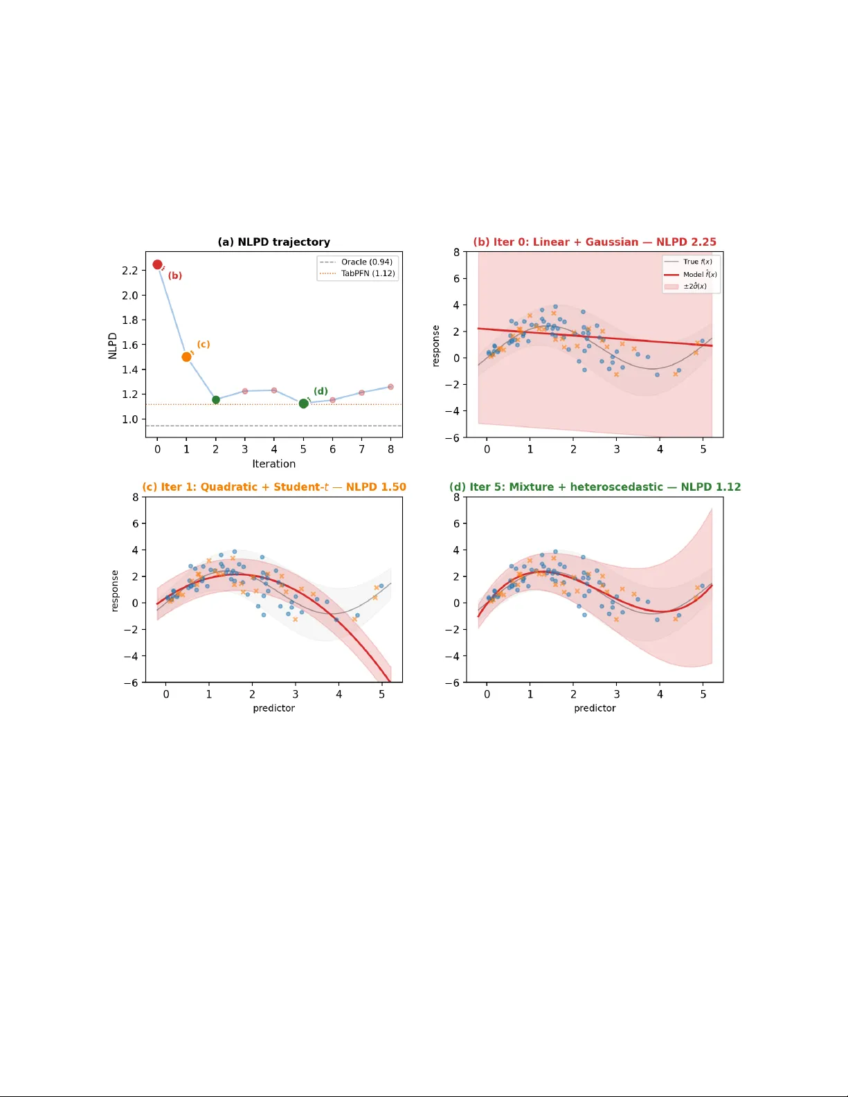
AutoStan: Autonomous Ba y esian Mo del Impro v emen t via Predictiv e F eedbac k Oliv er D ¨ urr Th urgau Institute for Digital T ransformation (TIDIT), Switzerland Marc h 31, 2026 Abstract W e presen t AutoStan, a framework in which a command-line interface (CLI) coding agent autonomously builds and iteratively impro ves Ba yesian models written in Stan. The agent op erates in a lo op, writing a Stan mo del file, executing MCMC sampling, then deciding whether to keep or revert each change base d on tw o complementary feedback signals: the negative log predictiv e densit y (NLPD) on held-out data and the sampler’s own diagnostics (divergences, R-hat, effectiv e sample size). W e ev aluate AutoStan on fiv e datasets with div erse modeling structures. On a syn thetic regression dataset with outliers, the agent progresses from naive linear regression to a mo del with Student- t robustness, nonlinear heteroscedastic structure, and an explicit con tamination mixture, matc hing or outp erforming T abPFN, a state-of-the-art black-box metho d, while remaining fully in terpretable. Across four additional experiments, the same mec hanism discov ers hierarchical partial p o oling, v arying-slop e mo dels with correlated random effects, and a Poisson attack/defense mo del for so ccer. No search algorithm, critic module, or domain-sp ecific instructions are needed. This is, to our knowledge, the first demonstration that a CLI co ding agent can autonomously write and iterativ ely improv e Stan co de for diverse Bay esian mo deling problems. 1 In tro duction Ba yesian mo deling is, in principle, b eautifully simple: y ou state what you b elieve ab out the data, condition on observ ations, and let probabilit y theory do the rest. In practice, this simplicit y was historically lo ck ed b ehind in tractable integrals—un til probabilistic programming languages like BUGS [ Lunn et al. , 2009 ], JAGS [ Plummer , 2003 ], and Stan [ Stan Developmen t T eam , 2017 ] made arbitrary generativ e mo dels accessible via MCMC. Y et even with Stan, the practitioner m ust still closely monitor and ”babysit” the inference: diagnose divergences, c heck R-hat and effective sample sizes, reparameterize funnels, tune priors, and iterate, a w orkflow that textb o oks like Gelman and Hill [ 2006 ] and McElreath [ 2020 ] ha ve made accessible but not less lab orious. The question w e tac kle in this pap er is whether mo dern CLI coding agents can automate parts of this tedious cycle. Karpath y’s autoresearch [ Karpathy , 2026 ] demonstrated that a co ding agent with a single scalar rew ard (v alidation bits-p er-b yte) can autonomously improv e a neural net work training script o vernigh t. W e translate this idea to Bay esian mo deling. Sup ervised Ba y esian inference is a natural fit for autonomous optimization b ecause it admits a principled, mo del-agnostic ev aluation metric lik e the negative log predictive density (NLPD) or any other strictly prop er scoring rule [ Gneiting and Raftery , 2007 ]. NLPD rewards calibrated predictive distributions and cannot b e gamed by ov er- or under-confiden t predictions, making it an ideal hands-off reward signal. The agent edits a Stan 1 mo del file, runs MCMC, observ es NLPD on held-out data, and decides whether to keep or revert. No additional orc hestration b ey ond the CLI agen t is needed. W e demonstrate AutoStan on five datasets spanning four statistical paradigms: regression with outliers, hierarc hical partial p o oling, v arying-slop e models, and sp orts mo deling. Eac h rev eals qualitativ ely different agent b ehaviors: from immediately writing the correct mo del (hierarc hical) to disco vering Student- t robustness for outlier handling and ultimately an explicit c on tamination mixture (regression). T o our knowledge, this is the first demonstration that a CLI co ding agent can autonomously write and impro v e Stan code. 2 Metho d 2.1 CLI Co ding Agen ts A CLI co ding agent is a terminal-based AI assistan t that can read and edit files, execute shell commands, and reason ab out their output in a read–edit–execute lo op. In our case, the agent edits Stan mo del files and executes MCMC via cmdstanpy [ CmdStanPy Developers , 2024 ]. Examples of CLI co ding agents include Claude Co de [ Anthropic , 2025 ], Gemini CLI [ Go ogle , 2025 ], Co dex CLI [ Op enAI , 2025 ], and op enco de [ op enco de con tributors , 2025 ], the last of which is op en-source. AutoStan relies on this capability but is not tied to any sp ecific agen t: any CLI co ding agen t that can edit files and execute shell commands can implement the optimization lo op. All exp eriments rep orted here use Claude Co de (v2.1.86) with Sonnet 4.6 (Mo del ID claude-sonnet-4-6) and a con text windo w of 200,000 tokens [ An thropic , 2025 ]. The framework, how ever, is agen t-agnostic and should w ork with an y mo dern CLI co ding agent. 2.2 W orkflo w The agen t is launched with a single prompt: Read program.md for your instructions. Your dataset is datasets/. Tw o files define the task: program.md con tains domain-agnostic Ba yesian w orkflo w instructions ( ∼ 56 lines; full text in App endix E ): read the data, inspect the training set, edit model.stan , run ev aluation, in terpret NLPD and diagnostics, decide whether to k eep or revert, rep eat. The instructions mention general strategies (non-cen tered parameterization, prior tuning, alternative likelihoo ds) but contain no dataset-sp ecific guidance. dataset.md is a short dataset description: column names, data format, the Stan data interface, and the dataset-sp ecific ev aluation command ( python evaluate.py ), which the agen t calls to compile the mo del, run MCMC, and receive the resulting NLPD. F or synthetic datasets, v ariable names are anonymized; the true generativ e process is nev er disclosed. Examples are given in App endix D and at https://github.com/tidit- ch/autostan . 2.3 Agen t Autonomy The agen t is free to explore the data b efore writing co de. In practice, it often computes summary statistics, c hecks for outliers, examines group structure, or insp ects v alue ranges on its own initiativ e, b eha vior that emerges from the agen t’s statistical reasoning rather than from any script. The agent 2 then writes a model.stan file with complete freedom ov er priors, likelihoo d, parameterization, and mo del structure. The only con tract: the mo del m ust output a log lik v ector in the generated quantities blo c k whic h is needed for the ev aluation script to compute the NLPD. 2.4 Ev aluation and Reward Eac h dataset has an evaluate.py script (executable but not readable by the agent) that compiles the mo del via cmdstanp y , runs MCMC (4 chains, 1 000 p ost-w armup draws for most datasets; 30 000 for the large 1D regression, to reduce Monte Carlo noise), computes NLPD from the log lik v ector (pro vided in the stan file). T est data is protected via filesystem permissions and nev er visible to the agen t. The primary reward is NLPD on held-out data: NLPD = − 1 N test N test X n =1 log 1 S S X s =1 p  y test n | θ ( s )  ! . (1) As a strictly prop er scoring rule [ Gneiting and Raftery , 2007 ], the NLPD is uniquely minimized b y the true predictiv e distribution. In con trast to metrics suc h as accuracy or RMSE, it p enalizes b oth errors in the predictive mean and miscalibrated uncertain t y . In principle, an y other strictly prop er scoring rule (e.g., CRPS) could b e used. The agen t halts after 3 consecutive non-improving iterations or 20 total. 3 Case Study: Regression with Outliers W e examine this case study in detail, as it clearly illustrates the core principles of our approach. Additional examples are pro vided in Section 4 . 3.1 Setup The agen t receiv es a dataset.md file (see App endix D ) containing the column names ( predictor , response ), the Stan data interface, and the ev aluation command, plus the one-line dataset descrip- tion: “Observ ations of a contin uous predictor and a contin uous resp onse.” The true generativ e pro cess, whic h is unkno wn to the agent, inv olv es three independent sources of difficult y: f ( x ) = 2 sin(1 . 2 x ) + 0 . 3 x, (2) σ ( x ) = 0 . 3 + 0 . 8 exp h − 1 2  x − 3 1 . 5  2 i , (3) and ∼ 6% of tr aining observ ations shifted ± 10–15 units as extreme outliers. The test set is dra wn from the clean generativ e pro cess (no outliers), so the oracle NLPD is simply the negative log-densit y under the true f ( x ) and σ ( x ); no mixture comp onent is needed. This oracle represen ts a lo wer b ound that cannot b e reac hed: b eyond the usual parameter uncertain ty from finite data, the oracle kno ws that the test set contains no outliers, an information the agent do es not hav e. W e ev aluate on t wo datasets: large ( n =500 train, 200 test) and small ( n =68 train, 30 test). 3 0 1 2 3 4 5 6 7 8 9 10 11 12 13 14 Iteration 1 . 2 1 . 4 1 . 6 1 . 8 2 . 0 2 . 2 NLPD (b) (c) (d) (a) NLPD trajectory ( n =500) Oracle (1.1442) T abPFN (1.2501) 0 1 2 3 4 5 − 4 − 2 0 2 4 6 response (b) Iter 0: Linear + Gaussian — NLPD 2.16 T rue f ( x ) ± 2 ˆ σ ( x ) Model ˆ f ( x ) 0 1 2 3 4 5 predictor − 4 − 2 0 2 4 6 response (c) Iter 1: Cubic + Student- t — NLPD 1.32 0 1 2 3 4 5 predictor (d) Iter 11: Sine + mixture + het. — NLPD 1.23 0 1 2 3 4 5 predictor (e) T abPFN — NLPD 1.2501 Figure 1: AutoStan on the large 1D regression dataset ( n = 500 train, 200 test; DGP defined in Section 3.1 ). In panels (b)–(d), the fitted mean ˆ f ( x ) is plotted with ± 2 ˆ σ ( x ) shaded; the faint grey ov erlay marks the oracle ground truth f ( x ) ± 2 σ ( x ). T raining p oin ts outside the plot range [ − 5 , 7] are shown as edge-pinned triangles ( ▲ / ▼ ) at the panel b oundary . (a) NLPD tra jectory o ver 15 iterations; colored mark ers iden tify the three mo del-fit panels. The dashed oracle line ( NLPD = 1 . 14) is a low er bound that cannot be reac hed (see Section 3.1 ). (b) Baseline (iter 0): Gaussian linear mo del; predictiv e bands are dominated by the ≈ 30 extreme training outliers ( NLPD = 2 . 16). (c) Iter 1: cubic p olynomial mean + Studen t- t lik eliho o d; one step eliminates most band inflation ( NLPD = 1 . 32). (d) Iter 11 (best): sinusoidal mean with learned frequency ω , heteroscedastic log-linear v ariance, and a con tamination-mixture likelihoo d; tight, lo cally calibrated bands closely follo w the oracle noise env elop e ( NLPD = 1 . 23). (e) T abPFN (90% predictiv e in terv al, NLPD = 1 . 25): mean tracking is accurate but in terv als are uniformly too wide—the model has absorb ed the training outliers, inflating uncertaint y across the full input range. 3.2 Mo del Evolution on the Large Dataset Figure 1 summarizes the large-dataset run in one view. In 15 iterations the age n t progresses from a flat, outlier-dominated baseline to a p osterior predictive that closely trac ks the true DGP (compare panels (b)–(d)), and ends up outp erforming T abPFN (panel (e)). The tra jectory reveals four key discov eries (see also T able 1 ): Disco very 1: Outlier Robustness ( ∆ = 0 . 84 ). The baseline linear regression with Gaussian errors scores NLPD = 2.16. At iteration 1, the agent adds a cubic p olynomial mean and switches to Studen t- t , a single change that drops NLPD by 0.84, the largest jump of the run. Disco very 2: Nonlinear Mean Structure ( ∆ ≈ 0 . 02 ). The agen t replaces the p olynomial with a sin usoidal basis a sin ( ω x ) + b cos ( ω x ) + cx (iter 2). It subsequen tly frees ω as a learnable 4 Iter NLPD Mo del ∆ 0 2.1589 Linear mean, Gaussian likelihoo d — 1 1.3181 Cubic p olynomial + Student- t − 0.84 2 1.3060 Sine basis + Student- t − 0.01 5 1.2854 + Quadratic log σ ( x ) − 0.02 7 1.2844 + Learnable frequency ω − 0.001 9 1.2325 Gaussian mixture (fixed σ out =10) − 0.05 11 1.2256 + Cubic log σ ( x ) − 0.007 T able 1: NLPD tra jectory , 1D regression large ( n = 500). Oracle NLPD = 1.1442. F ull tra jectory including rejected iterations in T able 4 . parameter (iter 7), reco v ering a v alue near the true frequency 1 . 2. Disco very 3: Heteroscedastic V ariance ( ∆ ≈ 0 . 02 ). Adding log σ ( x ) as a quadratic then cubic p olynomial captures the lo cally elev ated v ariance near x ≈ 3 (iters 5, 11). Disco very 4: Robust Mixture Mo del ( ∆ = 0 . 05 ). A t iteration 9 the agen t replaces Student- t with an explicit t w o-comp onen t Gaussian mixture: y ∼ (1 − π ) N ( µ ( x ) , σ ( x )) + π N ( µ ( x ) , σ out ) . (4) The p osterior estimate ˆ π ≈ 6% is close to the true contamination fraction. Ho wev er, introducing t w o exc hangeable mixture comp onents leads to a lab el-switching pathology: the p osterior is inv ariant under p erm utation of the comp onent lab els, effectively sw apping the roles of σ ( x ) and σ out . As a result, MCMC c hains alternate b et ween mo des in which either component explains the outliers, leading to p o or mixing (R-hat = 1.52 at iteration 10). The agent resolves this issue by fixing σ out = 10 based on data insp ection, thereby restoring stable inference. 3.3 Small Dataset ( n =68 ) With only n = 68 training observ ations, the same three di sco v eries o ccur in compressed form (9 iterations; see Appendix A.1 ): (1) outlier robustness via Studen t- t (∆ = 0 . 75), (2) nonlinear mean with heteroscedastic v ariance (∆ = 0 . 35), and (3) con tamination mixture (∆ = 0 . 03), reac hing NLPD 1.12. The sinusoidal frequency and cubic heteroscedastic profile, which require more data to iden tify , are absent here and cannot b e identified due to small sample size. 3.4 Comparison with T abPFN W e compare against T abPFN [ Hollmann et al. , 2025 ], a transformer pre-trained on syn thetic tabular data that claims to approximate Ba yesian inference without fitting a mo del at test time (details in App endix B ). Other natural baselines exist (gradient-bo osted trees [ Chen and Guestrin , 2016 ] or deep ensembles), but T abPFN is particularly useful out of the b ox as it pro duces full predictiv e distributions rather than p oin t estimates and is curren tly a state-of-the-art metho d for regression tasks. On the small dataset, T abPFN (NLPD 1.12) and AutoStan (NLPD 1.12) are effectively tied; on the large dataset, AutoStan slightly outp erforms T abPFN (1.23 vs. 1.25). The gap reflects structural adv antages: the sinusoidal mean captures the true functional form, the heteroscedastic v ariance gives lo cally calibrated uncertain ty , and the mixture correctly separates outliers. The main 5 adv antage, ho wev er, is in terpretabilit y: AutoStan exp oses every assumption (mean, v ariance profile, outlier fraction ˆ π ) with p osterior uncertaint y; T abPFN pro vides a predictive distribution but no explanation. 4 Additional Datasets The 1D regression serv es as a single illustrative example. T o assess how broadly the mechanism generalizes, within the limited scop e of this exploratory study , we apply AutoStan to four additional datasets spanning hierarc hical, v arying-slop e, and fo otball (soccer) modeling problems (T able 2 ; complete tra jectories in App endix A ). A large-scale b enchmark is b eyond the scop e of this pap er; our goal is instead to demonstrate the range of mo deling structures the agent can discov er. Hierarc hical: small ( n j = 8 , 20 groups). The generativ e structure follows the spirit of the classic Eigh t Schools mo del [ Rubin , 1981 ] (group means dra wn from a shared prior, observ ations drawn from those m eans), but uses a syn thetic dataset with anon ymized v ariable names to a void LLM con tamination. The agent selected a hierarc hical partial-p o oling mo del as its b aseline (NLPD = 1.50, oracle: 1.49), reac hing near-optimal p erformance already at iteration 0. Three attempted improv e- men ts (non-centered parameterization (NCP), Studen t- t , group-sp ecific σ ) all increased NLPD. The finding is the baseline c hoice itself: given anonymized group-structured data, the agent immediately wrote the correct mo del. Hierarc hical: large ( n j = 40 , 20 groups). Same generativ e pro cess, more data. The agent ac hieved four consecutive improv ements: NCP , group-sp ecific v ariances, Student- t lik eliho o d, and tigh ter data-informed priors, reaching NLPD 1.4014 (oracle: 1.4039). It also ran a principled ablation, rev erting to Normal lik eliho o d to confirm Studen t- t w as b eneficial. How ever, the b est mo del slightly outp erforms the oracle, a result that is not statistically meaningful and likely reflects mild o verfitting to the test set through iterativ e optimization (see Limitations). V arying slop es ( J = 15 groups). Generated from correlated random intercepts and slop es, with anon ymized v ariable names. The largest gain (∆ = 0 . 51) came from disco v ering v arying slop es at iter 1. Most strikingly , the agen t disco vered a piecewise linear structure not pr esent in the true gener ative mo del (iter 10), achieving NLPD 1.2738 vs. oracle 1.2627. While the gap is small, the piecewise structure is a mo deling artifact rewarded by the test set and is considered another instance of mild test-set adaptation through iterative optimization. The agent correctly recognized when additional complexit y b ecame counterproductive: 3-segmen t piecewise (15 div ergences) and learned knot p ositions (282 divergences, R-hat = 1.63) were b oth rejected. Bundesliga 2024/25 (real data). Real matc h results, 18 teams, temp oral train/test split. This is the only dataset with domain-lab eled column names ( home team id , home goals , etc.). The agent immediately applied a canonical Poisson mo del with separate attack and defense parameters, then iterativ ely added hierarchical priors (∆ = 0 . 020), NCP , and team-sp ecific home adv antage (∆ = 0 . 003). It rejected the negative binomial likelihoo d, the Dixon–Coles lo w-scoring correction [ Dixon and Coles , 1997 ], and a Bradley–T erry-style quality parameter [ Bradley and T erry , 1952 ], none of which impro ved NLPD. An earlier exp eriment with fully anonymized column names ( unit a , count a ) revealed the agent’s pattern recognition: from 18 units, small integer coun ts (0–7), and a paired-matc h up structure alone, 6 Hier. S Hier. L Slop es 1D S 1D L Bundes. Oracle 1.494 1.404 1.263 0.944 † 1.144 † — Baseline 1.500 1.404 1.818 2.248 2.159 1.566 Best 1.500 1.401 1.274 1.124 1.226 1.543 Gap 0.006 − 0.003 0.011 0.180 † 0.081 † — Iters 0 4 10 5 11 9 T able 2: Summary across all exp eriments. Gap = Best − Oracle (lo wer is b etter; negative means the mo del outp erforms the oracle, likely due to test-set ov erfitting). † Oracle is a strict low er b ound that cannot b e reached: the oracle knows the test set contains no outliers, whereas the agent must accoun t for the ≈ 6% training contamination. The agent exhibits qualitatively different b eha viors dep ending on dataset structure and size. it reasoned “ This lo oks like a sp orts-style matchup dataset ” and wrote a P oisson attac k/defense mo del as its baseline, without any domain lab els. 5 Related W ork A gro wing b o dy of work explores LLM-driven statistical mo deling. Li et al. [ 2024 ] structure their system around the classic iterative cycle of prop osing a mo del, fitting it, critiquing the fit, and revising. Implemen ted in PyMC, an LLM plays b oth roles: mo deler (prop osing probabilistic programs) and domain exp ert (critiquing them). Mo delSMC [ W ahl et al. , 2026 ] tak es a more formal route, recasting mo del discov ery as probabilistic inference with candidate mo dels as particles in a sequential Monte Carlo sampler; theoretically elegan t but substantially more complex. MA THMO [ Liu and v an der Sc haar , 2026 ] tak es a broader scop e, treating mathematical mo deling in general (not just probabilistic mo dels) as a sequential decision-making problem. Domk e [ 2025 ] sidesteps iterativ e improv ement en tirely: an LLM generates man y candidate probabilistic programs from an informal description, and predictions are computed as a w eighted av erage, i.e., Bay esian mo del a v eraging with an LLM prior o ver mo del space. A t the sp ecification end, LLM-BI [ Huang , 2025 ] demonstrates that LLMs can elicit priors and lik eliho o ds from natural language, though so far only for linear regression. All of these approac hes in tro duce dedicated infrastructure: custom critic mo dules, SMC samplers, mo del-space priors, or multi-ob jective search algorithms. AutoStan is radical in what it do es not need. The entire system consists of a generic CLI co ding agen t, a 56-line instruction file, a short dataset description, and NLPD as the sole rew ard: no custom framework, no search algorithm, no critic. Our direct inspiration is Karpathy’s autoresearc h [ Karpath y , 2026 ], which show ed that a co ding agent with a single scalar rew ard (v alidation bits-per-byte) can autonomously impro v e a neural netw ork training script o v ernight. AutoStan translates this to Ba yesian mo deling, where NLPD (a strictly prop er scoring rule) replaces bits-p er-byte and Stan mo del files replace Python training scripts. An extension is that AutoStan augments the scalar reward with the rich diagnostic output of the MCMC sampler (divergences, R-hat, and effective sample sizes), giving the agent a second feedbac k c hannel that signals not just whether a mo del impro v ed but ho w it is broken and what to fix next. The contrast with blac k-b o x metho ds is instructiv e. T abPFN [ Hollmann et al. , 2025 ], a transformer pre-trained on synthetic datasets, pro duces comp etitive predictive distributions, but no mo del: there are no parameters to in terpret, no priors to insp ect, no assumptions to challenge. AutoStan’s output is fundamentally different: a complete generative mo del in Stan with explicit lik eliho o d, 7 priors, and structure that a statistician can read, critique, and build up on. Moreo ver, b ecause the agen t runs in an interactiv e CLI, the practitioner can pause the lo op, ask the agent to explain its mo deling c hoices in plain language, request sp ecific changes, or resume autonomous improv ement; ev en a user who do es not read Stan fluently can ask the agent to translate the mo del into a verbal description of its assumptions, making the Bay esian workflo w acce ssible well b eyond the traditional exp ert comm unit y . 6 Discussion and Conclusion F our findings emerge across all exp eriments. (1) NLPD and MCMC diagnostics drive structural disco v ery : NLPD signals whether a change impro ves predictive p erformance, while the sampler’s output (div ergences, elev ated R-hat, p o or mixing) signals how a mo del is brok en and what to fix. Both channels are essential: the agent discov ered robust likelihoo ds, nonlinear heteroscedastic structure, con tamination mixtures, hierarchical p o oling, v arying slop es, and sp ort-sp ecific mo dels b y reading b oth, and the final output is not just a score but a complete, readable Stan mo del. (2) The agent adapts to data structure and scale : on small hierarc hical data it immediately writes the correct mo del; with more data it finds additional structure (group-sp ecific v ariances, learned frequencies). On the 1D regression, 68 observ ations suffice for outlier robustness; with 500, the agent also reco vers the true sinusoidal frequency and cubic heteroscedastic profile. (3) The agen t adapts to domain : anonymized v ariable names lead to generic baselines; domain-lab eled columns (Bundesliga) lead to domain-appropriate models (Poisson attack/defense). Ev en with fully anon ymized column names, the agen t’s w orld knowledge helps it recognize structural patterns (e.g., paired in teger counts as a sp orts match up). (4) The agen t kno ws when to stop : div ergences, elev ated R-hat, and increased NLPD serve as reliable stopping signals, and the agen t correctly rejects o vercomplex mo dels across all datasets. Limitations. Iterative NLPD optimization on a fixed test set risks mild o verfitting: on the hierarc hical-large dataset, the b est mo del slightly outp erforms the oracle (NLPD 1.401 vs. 1.404), and on v arying slop es, the agent disco v ers piecewise structure not in the true DGP . These results are not statistically meaningful impro vemen ts ov er the oracle but artifacts of optimizing against a finite test set ov er multiple iterations. A mitigation is cross-v alidation or p erio dic test-set rotation, though this increases computational cost. When no held-out test set is a v ailable, PSIS-LOO [ V ehtari et al. , 2017 ] offers a principled within-sample surrogate: it is computed directly from the log lik v ector. Because AutoStan pro duces insp ectable Stan co de, a human reviewer can alwa ys v erify whether a giv en improv ement reflects genuine statistical insigh t or test-set adaptation, an adv an tage absent from black-box metho ds. A similar issue can arise when the agen t uses exploratory data analysis to inform priors. E.g., centering an outlier-scale prior on magnitudes observed in the training data. This technically conflates prior and likelihoo d, but is acceptable when prediction is the primary goal, as the held-out test set remains an honest judge of predictive quality . F or users in terested in gen uine inference, the agent’s output is not a black b o x but readable Stan code: the data-informed priors can simply b e replaced with the analyst’s true prior b eliefs b efore a final sampling run. The agen t’s training data presents b oth adv an tages and limitations. On the one hand, it may ha ve encoun tered similar textbo ok problems, making it difficult to disen tangle gen uine statistical reasoning from memorization; w e mitigate this b y using anonymized syn thetic datasets with unpublished generativ e processes. On the other hand, domain knowledge is a strength: when the Bundesliga columns carry semantic lab els, the agen t readily selects an appropriate P oiss on attack/defense mo del, and even with fully anonymized columns it can recov er structural patterns from its training. 8 A CLI co ding agent, guided only by NLPD, autonomously disco vers sophisticated probabilistic mo dels across diverse datasets (regression, hierarc hical, v arying-slop e, and sp orts) while pro ducing fully in terpretable Stan co de. No searc h algorithm, critic, or domain-sp ecific tuning is required. NLPD and MCMC diagnostics are all you need. Co de, datasets, and Stan mo del snapshots are a v ailable at https://github.com/tidit- ch/ autostan . A Claude Co de skill for practical use on new data is a v ailable at https://github. com/tidit- ch/autostan- skill . 9 References An thropic. Claude code: An agen tic coding tool, 2025. URL https://code.claude.com/docs/ en/overview . Ralph A. Bradley and Milton E. T erry . Rank analysis of incomplete blo ck designs: I. the metho d of paired comparisons. Biometrika , 39(3/4):324–345, 1952. Tianqi Chen and Carlos Guestrin. X GBo ost: A scalable tree b o osting system. In Pr o c e e dings of the 22nd A CM SIGKDD International Confer enc e on Know le dge Disc overy and Data Mining , pages 785–794, 2016. CmdStanPy Developers. CmdStanPy: Python in terface to CmdStan, 2024. URL https://mc- stan. org/cmdstanpy/ . Mark J. Dixon and Stuart G. Coles. Modelling asso ciation fo otball scores and inefficiencies in the fo otball b etting market. Journal of the R oyal Statistic al So ciety: Series C (Applie d Statistics) , 46 (2):265–280, 1997. Justin Domke. Large language Ba y es. In A dvanc es in Neur al Information Pr o c essing Systems , 2025. URL . Andrew Gelman and Jennifer Hill. Data Analysi s Using R e gr ession and Multilevel/Hier ar chic al Mo dels . Cam bridge Universit y Press, 2006. Tilmann Gneiting and Adrian E. Raftery . Strictly prop er scoring rules, prediction, and estimation. Journal of the A meric an Statistic al Asso ciation , 102(477):359–378, 2007. Go ogle. Gemini CLI: An AI agent for the terminal, 2025. URL https://github.com/ google- gemini/gemini- cli . Noah Hollmann, Samuel M ¨ uller, Lennart Puruck er, Arjun Krishnakumar, Max K¨ orfer, Shi Bin Ho o, Robin Tib or Schirrmeister, and F rank Hutter. Accurate predictions on small data with a tabular foundation mo del. Natur e , 637:319–326, January 2025. doi: 10.1038/s41586- 024- 08328- 6. Y ongchao Huang. LLM-BI: T ow ards fully automated Bay esian inference with large language mo dels, 2025. URL . Andrej Karpathy . autoresearc h. GitHub, 2026. URL https://github.com/karpathy/ autoresearch . Mic hael Y. Li, Emily B. F o x, and Noah D. Go o dman. Automated statistical mo del discov ery with language mo dels. In Pr o c e e dings of the 41st International Confer enc e on Machine L e arning , Pro ceedings of Mac hine Learning Researc h, 2024. URL . T ennison Liu and Mihaela v an der Schaar. MA THMO: Automated mathematical mo deling through adaptiv e searc h. In Pr o c e e dings of the 14th International Confer enc e on L e arning R epr esentations , 2026. URL https://openreview.net/forum?id=t2fZ2GOwAT . Da vid Lunn, David Spiegelhalter, Andrew Thomas, and Nicky Best. The BUGS pro ject: Ev olution, critique and future directions. Statistics in Me dicine , 28(25):3049–3067, 2009. Ric hard McElreath. Statistic al R ethinking: A Bayesian Course with Examples in R and Stan . Chapman & Hall/CR C, 2nd edition, 2020. 10 Op enAI. Co dex CLI: A light weigh t coding agen t for the terminal, 2025. URL https://github. com/openai/codex . op enco de contributors. op enco de: Op en-source AI co ding agen t for the terminal, 2025. URL https://opencode.ai . Mart yn Plummer. JA GS: A program for analysis of Bay esian graphical mo dels using Gibbs sampling. In Pr o c e e dings of the 3r d International Workshop on Distribute d Statistic al Computing (DSC 2003) , 2003. Donald B. Rubin. Estimation in parallel randomized exp erimen ts. Journal of Educ ational Statistics , 6(4):377–401, 1981. Stan Developmen t T eam. Stan mo deling language users guide and reference man ual, version 2.17.0, 2017. URL https://mc- stan.org . Aki V ehtari, Andrew Gelman, and Jonah Gabry . Practical ba yesian mo del ev aluation using leav e- one-out cross-v alidation and W AIC. Statistics and Computing , 27(5):1413–1432, 2017. doi: 10.1007/s11222- 016- 9696- 4. Stefan W ahl, Raphaela Schenk, Ali F arnoud, Jakob H. Mack e, and Daniel Gedon. A probabilistic framew ork for LLM-based mo del discov ery , 2026. URL . 11 A Additional Results This app endix collects full iteration-by-iteration tra jectories for all exp eriments. Checkmarks ( ✓ ) denote accepted impro v ements; crosses ( × ) denote rejected attempts that were reverted. A.1 1D Regression: Small Dataset ( n =68 ) Figure 2: AutoStan on the 1D regression small dataset ( n = 68). (a) NLPD tra jectory o ver 9 iterations. (b) Baseline: linear + Gaussian, enormous bands from 4 extreme outliers. (c) Iter 1: quadratic mean + Studen t- t , the largest gain (∆ = 0 . 75). (d) Iter 5 (b est): cubic + log-linear σ ( x ) + con tamination mixture; NLPD 1.1244, matching T abPFN (1.1202) while remaining fully in terpretable. 12 Iter NLPD Model / change ∆ 0 2.2482 Baseline: linear mean, Gaussian likelihoo d — 1 1.5023 ✓ Student- t likelihoo d + quadratic mean − 0.746 2 1.1558 ✓ Cubic mean + log-linear σ ( x ) + Student- t − 0.347 3 1.2247 × F ourier basis mean (sin/cos) +0.069 4 1.2319 × Quartic mean + quadratic log σ +0.076 5 1.1244 ✓ Con tamination mixture ( ˆ π ≈ 6%) + log-linear σ ( x ) − 0.031 6 1.1520 × Student- t clean comp onent instead of Normal +0.028 7 1.2131 × Mixture + cubic+sin(x) mean + linear log σ +0.089 8 1.2592 × Mixture + quartic mean (centered at x =2) +0.135 T able 3: Complete tra jectory , 1D regression small ( n = 68). Oracle NLPD = 0.9443. T abPFN NLPD = 1.1202. A.2 1D Regression: Large Dataset ( n =500 ) The main b o dy (T able 1 ) shows only the 7 key accepted iterations. Here the full 15-iteration run is sho wn, including all rejections. The spik e at iter 10 (NLPD = 1.35) reflects lab el-switching when σ out w as estimated; the agent diagnosed this via R-hat = 1.52 and reverted to fixing σ out = 10. Iter NLPD Model / change ∆ 0 2.1589 Baseline: linear mean, Gaussian likelihoo d — 1 1.3181 ✓ Student- t + cubic p olynomial mean − 0.841 2 1.3060 ✓ Sine basis: a sin( π x/ 3)+ b cos( π x/ 3)+ cx − 0.012 3 1.3088 × 2-harmonic F ourier basis +0.003 4 1.2952 ✓ + Linear log σ ( x ) = s 0 + s 1 x − 0.011 5 1.2854 ✓ + Quadratic log σ ( x ) = s 0 + s 1 x + s 2 x 2 − 0.010 6 1.2859 × Sine+quadratic mean + quadratic log σ +0.001 7 1.2844 ✓ + Learnable frequency ω (recov ers ˆ ω ≈ 1 . 2) − 0.001 8 1.2635 ✓ Gaussian mixture ( ˆ π ≈ 10%), estimated σ out − 0.021 9 1.2325 ✓ Mixture, fixed σ out =10 (stabilizes lab el-switc hing) − 0.031 10 1.3529 × Estimated σ out (lognormal prior); R-hat = 1.52 +0.120 11 1.2256 ✓ Cubic log σ ( x ) , fixed σ out =10 − 0.007 12 1.2262 × Sine-based log σ ( x ) instead of cubic +0.001 13 1.2258 × Cubic log σ + seasonal adjustment +0.000 14 1.2291 × Studen t- t inlier + Normal(10) outlier mixture +0.004 T able 4: Complete tra jectory , 1D regression large ( n = 500). Oracle NLPD = 1.1442. T abPFN NLPD = 1.2501. A.3 Syn thetic Hierarchical Generated from µ j ∼ N (0 , 1), y ij ∼ N ( µ j , 1), J = 20 groups. V ariable names anonymized (“unit”, “effect”). 13 A.3.1 Small Dataset ( n j =8 , 160 train / 40 test) Iter NLPD Mo del 0 1.4999 Hierarchical centered, weakly informativ e priors ← b est 1 1.5014 Non-centered parameterization 2 1.5035 Student- t likelihoo d 3 1.5019 Group-sp ecific σ (ov erfit) T able 5: Complete tra jectory , hierarchical small ( n j =8). Oracle NLPD = 1.4935. A.3.2 Large Data set ( n j =40 , 800 train / 200 test) The agen t ran a principled ablation at iter 7, reverting to Normal likelihoo d to confirm Studen t- t w as b eneficial (+0 . 002 NLPD when remo v ed). Iter NLPD Model / change ∆ 0 1.4036 Hierarchical centered, shared σ — 1 1.4035 ✓ NCP for group means − 0.0001 2 1.4025 ✓ + Group-sp ecific σ (hierarchical log-normal) − 0.0010 3 1.4018 ✓ + Student- t likelihoo d ( ν estimated) − 0.0007 4 1.4014 ✓ + Tighter data-informed priors − 0.0004 5 1.4020 × Fixed ν =10 instead of estimated +0.0006 6 1.4015 × ν ∼ Gamma(2 , 0 . 2) (heavier prior) +0.0001 7 1.4034 × Normal likelihoo d ablation (confirms Student- t helps) +0.0020 T able 6: Complete tra jectory , hierarchical large ( n j =40). Oracle NLPD = 1.4039. A.4 V arying Slop es ( J =15 groups) Generated from α j ∼ N (2 , 1), β j ∼ N ( − 0 . 5 , 0 . 7), y ij ∼ N ( α j + β j x ij , 0 . 8), 25 obs/group (300 train / 75 test). Anon ymized column names. Iter NLPD Model / change ∆ 0 1.8178 Baseline: fully p o oled regression — 1 1.3091 ✓ V arying intercepts + slop es, NCP − 0.509 2 1.3073 ✓ + LKJ Cholesky correlation − 0.002 3 1.3073 ✓ + Student- t likelihoo d ( ν ∼ Gamma) < 0.001 4 1.3055 ✓ + Unit-sp ecific σ (hierarchical) − 0.002 5 1.2910 ✓ + Hierarchical quadratic term p er unit − 0.015 6 1.2933 × Indep endent slop es + intercepts + quadratic +0.002 7 1.2839 ✓ 3D LKJ ( α , β , γ ) correlated − 0.007 8 1.2861 × Tighter τ 3 ∼N (0 , 0 . 5) prior +0.002 9 1.2890 × LKJ(4) prior instead of LKJ(2) +0.005 10 1.2738 ✓ Piecewise linear at x =0 , 3D LKJ − 0.010 11 1.2833 × 3-segmen t piecewise (knots ± 1); 15 divergences +0.010 12 1.2949 × Piecewise + predictor-dep enden t σ ( x ) +0.021 13 1.2937 × Learned shared knot k ∼N (0 , 1); 282 divergences +0.020 T able 7: Complete tra jectory , v arying slop es ( J =15). Oracle NLPD = 1.2627. 14 A.5 Bundesliga 2024/25 Real match results, 18 teams, 207 training matc hes (matchda ys 1–23), 99 test matc hes (matchda ys 24–34). Domain-labeled column names. Iter NLPD Model / change ∆ 0 1.5663 Baseline: Poisson, indep endent priors — 1 1.5465 ✓ Hierarchical priors on attack/defense − 0.020 2 1.5557 × Negative binomial likelihoo d +0.009 3 1.5463 ✓ NCP (attack/defense raw) − 0.000 4 1.5472 × Dixon–Coles low-score correction +0.001 5 1.5468 × Correlated attack/defense ( ρ ∼N ( − 0 . 3 , 0 . 4)) +0.001 6 1.5460 ✓ NCP + tighter σ ∼N (0 , 0 . 5) priors − 0.000 7 1.5544 × Negative binomial home, Poisson aw ay +0.008 8 1.5645 × Single quality param p er team (Bradley–T erry style) +0.019 9 1.5432 ✓ T eam-sp ecific home adv an tage δ j − 0.003 10 1.5443 × Symmetric: δ h added/subtracted from b oth λ +0.001 11 1.5432 × Separate attac k/defense home adv antage < 0.001 12 1.5460 × ZIP + team home adv an tage ( π h ≈ 9%) +0.003 T able 8: Complete tra jectory , Bundesliga 2024/25. No oracle NLPD (real data). (a) T eam-sp ecific home adv an tage. (b) A ttac k vs. defense strength. Figure 3: Bundesliga mo del parameters (iteration 9). (a) Dortmund (0.39), F reiburg (0.33), Bay ern (0.32) b enefit most from pla ying at home; Heidenheim ( − 0.01) and St. Pauli (0.00) show no home adv antage. (b) Attac k vs. defense with 90% credible interv als; Ba yern’s dominance is clearly visible. B T abPFN Comparison Details T abPFN 2.2.1 [ Hollmann et al. , 2025 ] was run with n estimators=8 : since the pre-trained trans- former is sensitiv e to the order of training examples, T abPFN runs 8 forward passes with different random p ermutations of the training data and a v erages the resulting predictiv e distributions. This 15 is an ensemble within a single fixed pre-trained mo del, not 8 separately trained mo dels. T abPFN’s predictiv e output is a histogram (“bar distribution”) ov er a fixed grid of bins cov ering the resp onse range. T o compute NLPD, we need a con tin uous density rather than bin masses, so w e approximate the densit y at each test p oint via CDF finite-differencing with δ = 0 . 02: ˆ p ( y n | x n ) ≈ CDF( y n + δ ) − CDF( y n − δ ) 2 δ . (5) This giv es a properly normalized con tinuous density directly comparable to AutoStan’s Gaus- sian/mixture NLPD. T abPFN’s built-in pdf() metho d returns unnormalized bin masses and was not used. (a) Small dataset ( n =68). (b) Large dataset ( n =500). Figure 4: T abPFN predictions. On the large dataset, the in terv als widen globally near outliers instead of isolating them, explaining T abPFN’s higher NLPD (1.2501 vs. AutoStan’s 1.2256). C T ec hnical Details C.1 F ramew ork After the agen t edits model.stan , it calls a p er-dataset evaluate.py script, which internally uses cmdstanp y to compile the mo del and run CmdStan for MCMC sampling (4 chains × 1000 p ost- w armup dra ws; 30 000 for the large 1D regression to reduce Monte Carlo noise in NLPD). The script then computes NLPD from the log lik v ector and app ends a JSON record to log.jsonl , prin ting the NLPD and sampler diagnostics for the agent to read. The agent nev er sees the test data or the script’s implemen tation: evaluate.py is executable but not readable ( chmod 111 ). C.2 P ermissions T est data and generation scripts are protected via filesystem p ermissions: evaluate.py is executable but not readable ( chmod 111 ); test data and generation scripts hav e no access p ermissions ( chmod 000 ). The agen t can only execute the ev aluation script. C.3 Compute and T oken Usage All exp erimen ts w ere run interactiv ely on a MacBook Pro (Apple M2 Pro, 10-core CPU, 16 GB RAM). MCMC wall time p er iteration ranges from a few seconds for small datasets (hierarchical mo dels with n j = 8) to sev eral min utes for the large 1D regression ( n = 500, 30 000 draws), where individual iterations to ok up to ∼ 50 min utes due to the large num b er of draws required to reduce Mon te Carlo noise in NLPD. Across the six rep orted exp eriments, the agen t generated a total of 16 roughly 220 000 output tok ens and read approximately 20 million tokens from cache. The high cac he-read-to-output ratio reflects the structure of the lo op: at each iteration the agent re-reads the accum ulated conv ersation context (dataset description, previous Stan mo dels, NLPD history) but pro duces only a short plan and the revised model.stan . C.4 NLPD Computation NLPD = − 1 N test N test X n =1 log 1 S S X s =1 p  y test n | θ ( s )  ! , (6) where θ ( s ) are p osterior dra ws. Computed via logsumexp from Stan’s log lik output. D Dataset Sp ecifications D.1 1D Regression The 1D regression dataset is the main case study and the one from whic h the most conclusions are dra wn. Belo w is the verbatim dataset.md the agen t receives—this is the c omplete information pro vided, nothing more. The true generative pro cess is nev er disclosed. T rue generativ e pro cess (not shown to agent): f ( x ) = 2 sin (1 . 2 x ) + 0 . 3 x ; σ ( x ) = 0 . 3 + 0 . 8 exp  − 1 2  x − 3 1 . 5  2  ; ∼ 6% con tamination at ± 10–15 units. Small: 68 train / 30 test. Large: 500 train / 200 test. V erbatim dataset.md (large v ersion; small is identical except n ): # Dataset: 1D Regression (Large) ## Overview Observations of a continuous predictor and a continuous response. The goal is to predict ‘response’ for held-out test observations. This is a larger version of the dataset with more training data. ## Data Format ‘train.csv’ columns: - ‘predictor’ --- continuous predictor variable - ‘response’ --- continuous response variable (target) 500 training observations. 200 test observations (held out, not visible to the agent). ## Data Interface The evaluation script passes the following to Stan: int N train; int N test; vector[N train] predictor train; vector[N test] predictor test; vector[N train] response train; 17 vector[N test] response test; ## Evaluation python datasets/regression 1d large/protected/evaluate.py \ --notes "..." --rationale "..." Your model must output a ‘log lik’ vector of length ‘N test’ in the generated quantities block. Note: This dataset uses extended MCMC sampling (30,000 post-warmup iterations per chain) for precise NLPD estimation. D.2 All Other Datasets The remaining datasets follow the same dataset.md structure (Overview, Data F ormat, Data In terface, Ev aluation, log lik contract). The true generative parameters for the syn thetic datasets are giv en in the tra jectory tables in App endix A . F ull dataset.md files, generation scripts, and Stan mo del snapshots are av ailable at https://github.com/tidit- ch/autostan . E Agen t Prompt The complete program.md is the only b ehavioral sp ecification the agent receiv es (b eyond the dataset- sp ecific dataset.md ). The contrast is the p oint: 56 lines of generic Ba y esian workflo w instructions + a 6-line dataset description ⇒ a sophisticated probabilistic mo del. Note that the reading of testfiles is not p ossible due to filesystem p ermissions, w e just tell the agen t that the test set is hidden so that it do es not try to read it and wastes time on it. # AutoStan --- Agent Instructions You are an autonomous Bayesian modeling agent. Your task is to iteratively improve a Stan model to minimize NLPD (negative log predictive density) on a held-out test set. ## Workflow 1. Read the dataset description: Read datasets//dataset.md to understand the data, format, and evaluation procedure. 2. Check history: Before proposing any change, read results//log.jsonl to see the full NLPD history and what has been tried. 3. Read training data: Read datasets//train.csv to understand the data structure and values. 4. Edit model.stan: Modify the model --- you can change priors, likelihood, parameterization, model structure, anything. 5. Evaluate: Run the evaluation script as specified in dataset.md. Always pass --notes (what you changed) and --rationale (why, referencing previous iterations). 6. Interpret results: Read the printed NLPD and diagnostics. Decide whether to keep or revert the change. 7. Repeat: Propose the next change based on what you’ve learned. 18 ## Rules - NLPD is the only metric. Lower NLPD = better model. - log lik is the only interface contract. Your model.stan must always output a log lik vector in the generated quantities block. - Do NOT read any files in protected/. - Do NOT randomly perturb. Think like a statistician reasoning from evidence. Reference previous iterations. - The filesystem is your memory. All history is in results/ --- read it before acting. - Reason briefly about why you make each change. ## Strategies to Consider - Non-centered vs centered parameterization - Prior tightening or loosening - Different likelihood families (Normal, Student-t, etc.) - Adding or removing hierarchy levels - Reparameterization for better sampling efficiency - Covariate effects, interactions - Regularizing priors ## Stopping Rule Stop when any of these conditions is met: - 3 consecutive non-improving iterations - 20 total iterations (including baseline) When you stop, write results//report.md summarizing: best model, trajectory, NLPD table, and key insights. ## Getting Started If no results//log.jsonl exists yet, write a deliberately simple baseline model. Run it to establish the baseline NLPD, then start improving. 19