A Nonlinear Incremental Approach for Replay Attack Detection
Replay attacks comprise replaying previously recorded sensor measurements and injecting malicious signals into a physical plant, causing great damage to cyber-physical systems. Replay attack detection has been widely studied for linear systems, where…
Authors: Tao Chen, Andreu Cecilia, Lei Wang
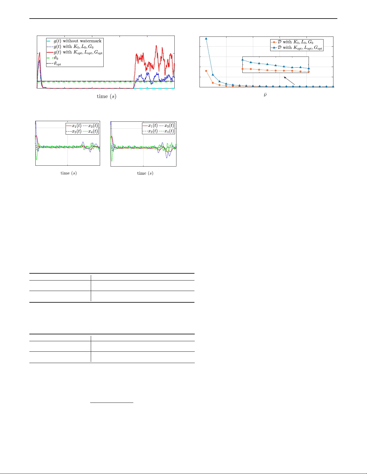
I 1 A Nonlinear Incremen tal Approac h for Repla y A ttac k Detection T ao Chen, Andreu Cecilia, Lei W ang*, Daniele Astol, Zhitao Liu Abstract— Repla y attac ks comprise replaying previously recorded sensor measuremen ts and injecting malicious signals in to a ph ysical plant, causing great damage to cyb er-ph ysical systems. Replay attack detection has b een widely studied for linear systems, whereas limited research has b een reported for nonlinear cases. In this pap er, the replay attac k is studied in the context of a nonlinear plant controlled b y an observer- based output feedbac k con troller. W e rst analyze repla y attac k detection using an innov ation-based detector and reveal that this detector alone ma y fail to detect such attac ks. Conse- quen tly , w e turn to a watermark-based design framework to impro v e the detection. In the prop osed framework, the eects of the watermark on attack detection and closed-lo op system p erformance loss are quantied by tw o indices, which exploit the incremen tal gains of nonlinear systems. T o balance the detection p erformance and control system performance loss, an explicit optimization problem is form ulated. Moreo ver, to ac hiev e a better balance, we generalize the prop osed w atermark design framework to co-design the watermark, con troller and observ er. Numerical simulations are presented to v alidate the prop osed frameworks. Index T erms— Cyber-physical systems, nonlinear systems, repla y attack detection, incremental gains. I . I N T R O D U C T I O N Cyb er-ph ysical systems (CPSs) seamlessly integrate computational algorithms with physical comp onents [1]. Suc h integrations rely on (wireless) comm unication net- w orks, raising securit y risks. T o analyze and improv e the resilience of CPSs to security risks, multiple types of attacks are studied in the literature, e.g., false data injection attac k [2], [3], replay attack [4], [5], den y-of- service attac k [6], [7], eav esdropping attack [8], etc. Among them, the replay attack has received signicant atten tion due to its simplicit y , stealthiness and model-free nature. F or attac k detection, one commonly used detector is the χ 2 detector [9], [10], which is innov ation-based, that is, it relies on the discrepancy b et w een the predicted and receiv ed sensor outputs. How ev er, as demonstrated in [4], [11], an innov ation-based detector may fail to detect repla y attac ks in the sense that, under some stability conditions, its detection rate conv erges to the false alarm rate. T o address this issue, lots of mechanisms hav e b een prop osed T ao Chen, Lei W ang and Zhitao Liu are with the College of Control Science and Engineering, Zhejiang Univ ersity , P .R. China (e-mail: tao_chen; lei.wangzju; ztliu@zju.edu.cn). Andreu Cecilia is with the Universitat P olitécnica de Cataluny a, A vinguda Diagonal, 647, 08028 Barcelona, Spain. (e-mail: andreu.cecilia@up c.edu).Daniele Astol is with the Univ. Lyon, Univ ersité Claude Bernard Lyon 1, CNRS, LAGEPP UMR 5007, F-69100 Villeurbanne, F rance (e-mail: daniele.astol@univ-lyon1.fr). Corresponding author: Lei W ang in the literature, which can b e broadly classied into t w o categories. The rst inv olves “enco ding-deco ding” the sensor measuremen t to b e repla y ed. Sp ecically , these metho ds use a random pair (e.g., tw o identical random n um bers) to encode the sensor measurements to b e trans- mitted and then deco de it at the receiv er’s side [12]– [14]. Under a repla y attac k, the detection is facilitated b y the mismatch of the random pair. Ho wev er, to achiev e sync hronization of the random pair, prior information a v ailable to both sides [12], [13] or an extra comm unication c hannel [14] is required, which reduces the applicability and the inherent robustness against adv ersaries [15]. An alternative to detect a replay attack is to add a “w atermark” [4] to the control input and stimulating the ph ysical plant. Under a replay attac k, the incoherence b et w een the expected stim ulation and the actual sen- sor measurements facilitates the repla y attac k detection. Nonetheless, since the watermark is essentially a distur- bance directly acting on the physical plan t, it inevitably aects the control system p erformance. Therefore, b oth detection performance and control system p erformance loss are considered when designing a watermark. In [4], the detection p erformance is ev aluated by the dierence b etw een the healthy innov ation cov ariance and the attac k ed one, while the system p erformance loss is ev aluated by the watermark-induced extra linear- quadratic-Gaussian (LQG) cost. Then, based on these ev aluations, an optimization problem is constructed in [11] to balance these tw o factors. Motiv ated b y these results, v arious strategies hav e b een rep orted to further reduce the control system p erformance loss or, equiv alently , to enhance detection p erformance with the same amount of w atermarking. F or example, [16] prop oses a p erio dic w atermarking sc heduling approach. In [17], a parsimo- nious policy is prop osed to limit the a v erage num ber of watermarking even ts. In [18], an ev en t-based physical w atermark is designed, where the probability of adding the w atermark is determined b y the inno v ation. In [19], sensitiv e states are considered, and additional constraints are dev eloped to strictly limit the eect of the watermark on these states. Moreo v er, n umerous w atermark design metho ds ha v e b een developed to achiev e specic objectives in replay attack detection, e.g., minimizing the av erage detection delay [17], making the w atermark unpredictable [20], extending the watermark for industrial pro cess op- eration optimization of cyb er-physical systems [21], and automatically learning and recognizing repla y attac ks [22]. 2 I T o sum up, w atermark approaches ha v e b een widely used to enhance χ 2 detectors. Moreov er, the detection p erformance and the con trol system performance loss ha ve b een well quan tied and balanced. How ever, all of these studies hav e b een conducted in the context of linear systems, and it is not straightforw ard to extend these metho ds to nonlinear cases. F or example, in [4], [16], [18]–[20], the detection p erformance is ev aluated by the dierence b etw een the attac k ed and the healthy innov ation co v ariance, which can b e explicitly computed for linear cases, but is signican tly more complex in nonlinear scenarios. In view of the ab ov e discussion, in this work, we study the repla y attac k detection problem for nonlinear systems. Sp ecically , we rst analyze the detection p erformance with an innov ation-based detector and sho w that, by itself, it ma y fail to detect suc h attacks. W e therefore adopt a watermark-based design framework. T o ev aluate the detection p erformance and con trol system performance loss, we employ incremental gain-based metho ds, which are broadly applicable in nonlinear scenarios. F urther- more, incremen tal gains allo w us to b ound the output (or state) of a system without requiring explicit calculation of v ariable distributions and indep endently of the sys- tem’s equilibrium point. With these ev aluations, sucient conditions for sp ecic detection performance and con trol system p erformance loss can b e rigorously established and exploited, which supp ort the watermark design. The main con tributions are summarized as follows. • A new w atermark design framework for nonlinear systems replay attack detection is prop osed, where the detection performance and the con trol system p erformance loss caused by the watermark are ev alu- ated by some indices that are induced by incremental gains. • Sucien t conditions for sp ecic detection p erfor- mance and con trol system performance loss are estab- lished, thereb y enabling the construction of a solv able optimization problem for the watermark design. • A systematic approach based on LMIs for co- designing the watermark, the controller and the observ er is further developed to achiev e a b etter tradeo b etw een the detection p erformance and the con trol p erformance loss. • F or detection p erformance ev aluation, a low er b ound b et w een the input dierence and the output dierence for nonlinear systems is required. Ho w ever, this index, referred to as the incremental L − 2 gain and denoted as L − δ 2 , has not been well dev elop ed in the literature. Extending the L − 2 gain to L − δ 2 and developing its corresp onding Lyapuno v (Prop osition 2) and LMI (Lemma 2) c haracterizations are t w o con tributions of the work. • The connection b etw een detection p erformance and L − δ 2 gain is not straightforw ard. Establishing a clear link b et w een the detector and the L − δ 2 gain for eec- tiv e p erformance ev aluation is another contribution. Notation. W e denote by N the set of natural num b ers, R n the set of real n umbers of dimension n ∈ N , R ≥ 0 the set of non-negativ e reals, R > 0 the set of p ositive reals. F or a vector x ∈ R n , ∥ x ∥ denotes the Euclidean norm and ∥ x ∥ Λ := √ x ⊤ Λ x for Λ ∈ R n × n . F or random vector x , x ∼ N ( µ, Σ) denotes that x follows a Gaussian distribution with mean µ and cov ariance Σ . F or column vectors x ∈ R m and y ∈ R n , col ( x, y ) := [ x ⊤ , y ⊤ ] ⊤ . F or matrix A ∈ R n × n , λ max ( A ) denotes the largest eigenv alue of A ( λ min ( · ) for the minimum). F or matrices A ∈ R m × m and B ∈ R n × n , diag ( A, B ) denotes a matrix with A and B in the main diagonal and 0 everywhere else. I n denotes iden tity matrix of dimension n × n . F or real-v alued Leb esgue integrable functions f : R ≥ t 0 → R n , ∥ f ∥ L 2 := R ∞ t 0 ∥ f ( t ) ∥ 2 d t for some t 0 ∈ R ≥ 0 . Given a function u : R ≥ 0 → R m , we dene ∥ u ( · ) ∥ ∞ = sup t ∈ [0 , ∞ ) ∥ u ( t ) ∥ . Given a signal u : R [0 , ∞ ) → R m and a scalar τ ∈ [0 , ∞ ) , w e denote by ( u ( t )) τ the τ - truncation of u ( t ) dened as ( u ( t )) τ = u ( t ) for all t ∈ [0 , τ ] and ( u ( t )) τ = 0 , for all t > τ . A mapping f : R p → R q is C n if it is n -times contin uously dieren tiable. In addition, a contin uous function α : R ≥ 0 → R ≥ 0 is of class K , if it is strictly increasing and α (0) = 0 . A contin uous function β : R ≥ 0 × R ≥ 0 → R ≥ 0 is of class KL if, for eac h xed s ≥ 0 , the function β ( · , s ) is of class K and, for each xed r > 0 , β ( r , s ) is strictly decreasing and lim r →∞ β ( r , s ) → 0 . I I . P R E L I M I N A R I E S O N I N C R E M E N TA L G A I N P R O P E RT I E S Consider a system of the form ˙ x = f ( x ) + B u, y = C x + D u (1) where f : R n → R n is a (lo cally) Lipschitz function satisfying f (0) = 0 , x ∈ R n is the state, u : [0 , ∞ ) → R m is a measurable and lo cally essentially bounded function taking v alues on a set of U ⊂ R m con taining the origin, and y ∈ R p the output. F urthermore, w e denote by X ( t, x 0 , u ) the unique solution of system (1) at time t , with initial state x 0 ∈ R n and input u ( t ) ∈ U . Similarly , we denote b y Y ( t, x 0 , u ) = C X ( t, x 0 , u ) + D u ( t ) its output tra jectory . F or system (1), w e provide the denitions of input-to- state stable [23], denoted as ISS, and incremen tal input- to-state stable [24], denoted as δ ISS. Denition 1 (ISS). System (1) is said to be input-to-state stable (ISS) if there exist α ∈ K and β ∈ K L suc h that the following holds for all t ≥ 0 ∥ X ( t, x 0 , u ) ∥ ≤ β ( ∥ x 0 ∥ , t ) + α ( ∥ u ( · ) ∥ ∞ ) (2) for any x 0 ∈ R n and u ( t ) ∈ U . Denition 2 ( δ ISS). System (1) is said to b e incrementally input-to-state stable if there exist α ∈ K and β ∈ KL such that the following holds for all t ≥ 0 ∥ X ( t, x 1 , u 1 ) − X ( t, x 2 , u 2 ) ∥ ≤ β ( ∥ x 1 − x 2 | , t ) + α ( ∥ u 1 ( · ) − u 2 ( · ) ∥ ∞ ) for any x 1 , x 2 ∈ R n and u 1 ( t ) , u 2 ( t ) ∈ U . A NONLINEAR INCREMENT AL APPROA CH F OR REPLA Y A TT ACK DETECTION 3 Next, based on [25], [26], we dene the incremental L + 2 gain, denoted as L + δ 2 . Denition 3 ( L + δ 2 gain). The L + δ 2 gain of system (1) is dened as L + δ 2 := inf γ + , if there exist γ + < ∞ and α + ∈ K suc h that for all t ≥ 0 and τ ≥ 0 , ∥ (( Y ( t, x 1 , u 1 ) − Y ( t, x 2 , u 2 )) τ ∥ L 2 ≤ γ + ∥ ( u 1 ( t ) − u 2 ( t )) τ ∥ L 2 + α + ( ∥ x 1 − x 2 ∥ ) (3) holds for any x 1 , x 2 ∈ R n and u 1 ( t ) , u 2 ( t ) ∈ U . In the following, w e also use [ L + δ 2 ] u y to indicate the input and output with resp ect to which the L + δ 2 gain is dened. With the denition of L + δ 2 , an upp er b ound on the L + 2 norm of the error b etw een tw o dierent output tra jectories of system (1) can b e eectiv ely estimated. Corresp ondingly , to get a low er b ound, we turn to the L − δ 2 gain, which is an incremental version of the L − 2 gain [27]. The formal denition of the L − δ 2 gain is provided b elo w. Denition 4 ( L − δ 2 gain). The L − δ 2 gain of system (1) is dened as L − δ 2 := sup γ − , if there exist γ − > 0 and α − ∈ K suc h that for all t ≥ 0 and τ ≥ 0 , ∥ (( Y ( t, x 1 , u 1 ) − Y ( t, x 2 , u 2 )) τ ∥ L 2 ≥ γ − ∥ ( u 1 ( t ) − u 2 ( t )) τ ∥ L 2 − α − ( ∥ x 1 − x 2 ∥ ) (4) holds for any x 1 , x 2 ∈ R n and u 1 ( t ) , u 2 ( t ) ∈ U . Remark 1. Note that for system (1) δ ISS implies an L + δ 2 gain b ecause the output is linear (this may b e not hold for generic nonlinear functions). Ho wev er, the con v erse is true only under additional (dieren tial) detectability conditions. Remark 2. Incremen tal properties, such as those consid- ered in this section, relate the state and output dierences b et w een any pair of the system’s tra jectories with distinct initial states and inputs. As extensiv ely studied in the literature (e.g. [24], [28]) one has the implications δ ISS ⇒ ISS and L + δ 2 gain ⇒ L 2 gain, while the con verse generically do es not hold true. In view of the previous denitions, w e no w pro vide tw o Ly apuno v c haracterizations of the L + δ 2 and L − δ 2 gains. The pro of of the former can b e found in [26, App endix B.1], while the pro of of the latter is p ostp oned to App endix A. Concerning the Lyapuno v characterization of δ ISS w e refer to [24]. Prop osition 1 (Lyapuno v L + δ 2 c haracterization). Suppose there exist a C 1 function V + : R n × R n × R → R ≥ 0 , functions α + , α + ∈ K ∞ and γ + > 0 suc h that α + ( ∥ x 1 − x 2 ∥ ) ≤ V + ( x 1 , x 2 , t ) ≤ α + ( ∥ x 1 − x 2 ∥ ) (5) ∂ V + ∂ t ( x 1 , x 2 , t ) + ∂ V + ∂ x 1 ( f ( x 1 )+ B u 1 )+ ∂ V + ∂ x 2 ( f ( x 2 )+ B u 2 ) ≤ γ + ∥ u 1 − u 2 ∥ 2 − ∥ y 1 − y 2 ∥ 2 (6) for all t ≥ 0 , x 1 , x 2 ∈ R n , and u 1 , u 2 ∈ U . Then the L + δ 2 gain of system (1) satises [ L + δ 2 ] u y ≤ γ + . Prop osition 2 (Lyapuno v L − δ 2 c haracterization). Suppose there exist a C 1 function V − : R n × R n × R → R ≥ 0 , functions α − , α − ∈ K ∞ and γ − > 0 suc h that α − ( ∥ x 1 − x 2 ∥ ) ≤ V − ( x 1 , x 2 , t ) ≤ α − ( ∥ x 1 − x 2 ∥ ) (7) ∂ V − ∂ t ( x 1 , x 2 , t ) + ∂ V − ∂ x 1 ( f ( x 1 )+ B u 1 )+ ∂ V − ∂ x 2 ( f ( x 2 )+ B u 2 ) ≤ − γ − ∥ u 1 − u 2 ∥ 2 + ∥ y 1 − y 2 ∥ 2 (8) for all t ≥ 0 , x 1 , x 2 ∈ R n , and u 1 , u 2 ∈ U . Then the L − δ 2 gain of system (1) satises [ L − δ 2 ] u y ≥ γ − . Finally , for systems of form (1), if w e assume that f : R n → R n is C 1 , w e can provide matrix inequality c haracterizations of the previous incremen tal gains, whic h will b e useful in the subsequen t developmen t of a compu- tationally viable design methodology . A matrix inequality characterization for the [ L + δ 2 ] u y gain follo ws from [26, Corollary 14], and is recalled in the next Lemma. F or con venience, dene A x := ∂ f ∂ x ( x ) . Lemma 1. Supp ose there exist a symmetric p ositive denite matrix P ∈ R n × n and γ + ≥ 0 satisfying A ⊤ x P + P A x + C ⊤ C P B + C ⊤ D ⋆ D ⊤ D − γ + I m ⪯ 0 , (9) for all x ∈ R n . Then, V + ( x 1 , x 2 ) = ( x 1 − x 2 ) ⊤ P ( x 1 − x 2 ) satises (5), (6) and system (1) has an incremental L + δ 2 gain [ L + δ 2 ] u y ≤ γ + . Motiv ated by the previous result, we prop ose a similar c haracterization for the [ L − δ 2 ] u y gain in the next Lemma. Lemma 2. Suppose there exist a symmetric negativ e denite matrix Q ∈ R n × n and γ − ≥ 0 satisfying A ⊤ x Q + QA x + C ⊤ C QB + C ⊤ D ⋆ D ⊤ D − γ − I m ⪰ 0 (10) for all x ∈ R n . Then, V − ( x 1 , x 2 ) = − ( x 1 − x 2 ) ⊤ Q ( x 1 − x 2 ) satises (7), (8) and system (1) has an incremental L − δ 2 gain [ L − δ 2 ] u y ≥ γ − . The pro of of Lemma 2 is p ostp oned to Appendix B. Remark 3. F rom (10), it is evident that if D = 0 , then γ − is alwa ys 0 . T o obtain a p ositive γ − , the relative degree of system (1) b etw een u and y must b e 0 . F or systems whose relative degree is greater than 0 , one can reduce its relativ e degree to 0 by redening a new output to include an auxiliary direct c hannel [27]. I I I . P R O B L E M F O R M U L A T I O N A. System Description Consider contin uous-time nonlinear plants of the form Σ np : ( ˙ x = f ( x ) + B u + ω y = C x + D u + ν, (11) 4 I where x ∈ R n is the plan t state, u ∈ R m is the input signal, y ∈ R p is the sensor measurement, and ω ∈ R n and ν ∈ R p are the system and sensor measuremen t noise, resp ectiv ely , which are assumed to b e Lebesgue in tegrable and b ounded as ∥ ω ∥ ∞ ≤ ω and ∥ ν ∥ ∞ ≤ ν with ω > 0 and ν > 0 . Finally , f : R n → R n is C 1 . F urthermore, we denote by X ( t, x 0 , u, ω ) the unique solution of system (11) at time t , with initial states x 0 ∈ R n and sub ject to the input u and noise ω . Similarly , we denote by Y ( t, x 0 , u, ω , ν ) = C X ( t, x 0 , u, ω ) + D u ( t ) + ν ( t ) its output tra jectory . F or conv enience, we omit the noise signal ω and ν and use notations X ( t, x 0 , u ) and Y ( t, x 0 , u ) in the following. F or output feedback con trol purp ose, we assume that a Luen b erger-t ype observer [29], [30] and a state feedback con troller are deploy ed, taking the form of Σ o : ( ˙ ˆ x = f ( ˆ x ) + B u + L ( y − ˆ y ) ˆ y = C ˆ x + D u, (12) and Σ c : u = κ ( ˆ x ) + v (13) resp ectiv ely , where ˆ x ∈ R n and ˆ y ∈ R p are the estimated state and output, resp ectively , L ∈ R n × p is the gain of observ er, κ : R n → R m is a Lipsc hitz feedbac k map, that is, there exists a constan t l κ > 0 suc h that ∥ κ ( x 1 ) − κ ( x 2 ) ∥ ≤ l κ ∥ x 1 − x 2 ∥ , (14) for all x 1 , x 2 ∈ R n , and v denotes a residual control signal to b e addressed later. W e denote b y b X ( t, ˆ x 0 , v , y ) and b Y ( t, ˆ x 0 , v , y ) = C b X ( t, ˆ x 0 , v , y ) + D u the solution and the output tra jectory of the observ er (12), resp ectively . Dene ˜ x := x − ˆ x as the observ ation error, whose dynamics are given as follows ˙ ˜ x = f ( x ) − f ( x − ˜ x ) + L ˜ y + ω , ˜ y = C ˜ x + ν (15) where u = κ ( x − ˜ x ) + v . W e denote by e X ( t, x 0 , v , y ) = X ( t, x 0 , u ) − b X ( t, ˆ x 0 , v , y ) the solution and e Y ( t, x 0 , v , y ) = Y ( t, x 0 , u ) − b Y ( t, ˆ x 0 , v , y ) the output tra jectory of (15), resp ectiv ely , where x 0 := col ( x 0 , ˆ x 0 ) . In addition, with the controller (13), the ph ysical plan t (11) evolv es as follows ˙ x = f ( x ) + B ( κ ( x − ˜ x ) + v ) + ω . (16) Then, we assume that the error dynamic system (15) and the controlled plant (16) and satisfy input-to-state stabilit y (ISS) prop erty [24], [31]. That is, Assumption 1. The error dynamic system (15) is ISS w.r.t. inputs ν and ω (see Denition 1) uniformly on x , and the controlled plant (16) is δ ISS w.r.t. inputs ˜ x, v , ω (see Denition 2). Designing con trollers and observ ers to ac hieve Assump- tion 1 has b een w ell studied, see for instance [32], and a metho dology can b e found in Lemma 3. Remark 4. W e analyze the nonlinear system of the form (11) and assume a linear output, as b oth choices are necessary to dev elop computationally tractable conditions. While parts of this theory might extend to more gen- eral (e.g., non-smo oth) systems or those with nonlinear outputs, these generalizations would likely preven t the tractable LMI characterizations for L − δ 2 and L + δ 2 gains presen ted in Lemmas 1 and 2. F or instance, a nonlinear output w ould lik ely require state-dep endent matrices P ( x ) and Q ( x ) , rendering the conditions intractable. B. Communication T opology and Repla y Attac k In practice, for remote con trol purp ose, the controller and observ er ma y be deploy ed in a remote control cen ter. In this case, as sho wn in Fig. 1, the sensor measurement y and the con trol signal u are transmitted through netw orks, making them susceptible to attac ks. Controller Observer Plant y y u ˆ x Network Network Attacker y a u a Plant layer Control layer Network layer Control center Fig. 1. Sc heme of the communication top ology . In this pap er, w e supp ose that the netw ork suers from a replay attack, and is free from delays and noise for simplicit y . The follo wing resources are supp osed to be a v ailable to the adv ersary: (i) The adversary can monitor and record the sensor measuremen t y for all time t . (ii) The adv ersary can arbitrarily mo dify the transmitted signals u and y to u a and y a , resp ectively . With the ab ov e resources, the replay attack strategy is giv en as follows. 1) (Record) F rom time 0 to time T , the adversary records a sequence of sensor measurements y . 2) (Repla y) F rom time T to time 2 T , the adversary repla ys the recorded sensor measuremen ts to tamp er the true sensor outputs, i.e., y a ( t ) = Y ( t − T , x 0 , u ) , T ≤ t < 2 T . (17) 3) (Con tamination) During replay , the adversary con- taminates the nominal control signal with a series of malicious control sequences u a to damage the plan t. Remark 5. F rom the attack er’s p ersp ective, one of the main benets of repla y attacks is their simplicity and the p ossibility of executing them without any system kno wledge. F or this reason, w e assume that the attack er A NONLINEAR INCREMENT AL APPROA CH F OR REPLA Y A TT ACK DETECTION 5 has no system kno wledge, in particular no knowledge of the watermarking signal. Before presenting the main detection mec hanism of this w ork, w e state the last assumption. W e assume that the repla y attack occurs when the system, and in particular its observ er, has already reached a steady state. Otherwise the replay ed signal will not b e consistent with the mo del and can b e easily detected. Assumption 2. The observer (12) has already reached its steady state at time instan t 0 . That is, we hav e ∥ e X ( t, x 0 , v , y ) ∥ ≤ α ω ( ∥ ω ( s ) ∥ ∞ ) + α ν ( ∥ ν ( s ) ∥ ∞ ) , for all t ≥ 0 , where α ω , α ν ∈ K . In this pap er, we fo cus on the repla y attack detection problem for nonlinear systems describ ed b y plant (11), observ er (12) and con troller (13). F or linear systems, it has b een sho wn that the innov ation-based detector is not sucien t for replay attack detection under some stability conditions (see [4], [11]), and thus the watermark-based detection is employ ed [4], [11], [16]–[22]. Motiv ated by these works, we consider the follo wing tw o problems. P1) F or nonlinear systems (11), (12) and (13), is the inno v ation-based detector sucien t for repla y attac k detection? P2) If the inno v ation-based detector is not sucient, how can w e dev elop a systematic w atermark-based repla y detection metho d for nonlinear systems? I V . I N N OVA T I O N - B A S E D R E P L A Y A T T AC K D E T E C T I O N In this section, we aim to answer the P1) b y revealing conditions under which the innov ation-based detector ma y fail to detect the repla y attac k. Sp ecically , the detector is assumed to hav e access to the sensor measurement y (or y a if under attack) and its estimation ˆ y , taking the form of Σ d : ψ = ( A ttac k , g ( t ) > ϑ No Attac k , g ( t ) ≤ ϑ g ( t ) := 1 σ Z t t − σ ∥ e Y ( s, x 0 , v , y ) ∥ 2 ds (18) where g ( t ) is referred to as the monitoring signal of the detector, e Y ( s, x 0 , v , y ) is the innov ation tra jectory given b y (15), and σ ∈ R > 0 is the window size. In the following, w e say that the detector is triggered if ψ = A ttac k. Remark 6. The detector (18) is a mo dication of the well- kno wn χ 2 detector [9], [10], which is widely used in CPSs and takes the form Σ χ : ψ χ = ( A ttac k , g χ ( t ) > ϑ χ No Attac k , g χ ( t ) ≤ ϑ χ g χ ( t ) = 1 σ Z t t − σ ∥ e Y ( s, x 0 , v , y ) ∥ 2 P − 1 ds (19) where P is the v ariance of the inno v ation for normalization and ϑ χ > 0 is the threshold. F or nonlinear systems, the inno v ation v ariance is generally nontrivial to compute, and th us we omit the normalization in (19) and employ (18). Under the replay attack, at time t ∈ [ T , 2 T ) , the observ er evolv es as follo ws, ˙ ˆ x = f ( ˆ x ) + B ( κ ( ˆ x ) + v ) − L [ C ˆ x + D ( κ ( ˆ x ) + v )] + Ly a ˆ y = C ˆ x + D ( κ ( ˆ x ) + v ) (20) where y a is the replay ed data given in (17). W e denote b y b X ( t, ˆ x T , v , y a ) and b Y ( t, ˆ x T , v , y a ) := C b X ( t, ˆ x T , v , y a ) + D ( κ ( b X ( t, ˆ x T , v , y a )) + v ) the solution and output tra jec- tory of observer (20) with initial state x T ∈ R n and sub ject to the repla y attac k y a . In addition, the inno v ation tra jectory under attac k is denoted as e Y ( t, x 0 , v , y a ) := Y ( t − T , x 0 , u ) − b Y ( t, ˆ x T , v , y a ) , with x 0 := col ( x 0 , ˆ x T ) . Then, the following prop osition summarizes a scenario where the detector ma y fail to detect the repla y attac k. Prop osition 3. Consider the system (11) with observer (12), controller (13) with v ( t ) = 0 , ∀ t ∈ R ≥ 0 , detector (18) and supp ose that Assumption 1 holds. Then, if σ ≤ T and (20) is δ ISS with input y a and state ˆ x , there exists a KL function β such that g ( t ) ≤ 1 σ Z T t − σ ∥ e Y ( s, x 0 , v , y ) ∥ 2 ds + 1 σ Z t T ∥ e Y ( s − T , x 0 , v , y ) ∥ 2 ds + β ( ∥ ˆ x ( T ) − ˆ x (0) ∥ , t ) , t ∈ [ T , T + σ ) , g ( t ) ≤ 1 σ Z t t − σ ∥ e Y ( s − T , x 0 , v , y ) ∥ 2 ds + β ( ∥ ˆ x ( T ) − ˆ x (0) ∥ , t ) , t ∈ [ T + σ, 2 T ) . (21) The pro of is postp oned to App endix C. Prop osition 3 sho ws that, if v ( t ) = 0 , ∀ t ∈ R ≥ 0 and (20) is δ ISS, the detector (18) is insucient for reliably detecting replay attacks. Specically , b ecause all of the inno v ation terms e Y ( t, x 0 , v , y ) in (21) are integrated ov er t ∈ [0 , T ) and the replay o ccurs since time instant T , the monitoring signal g ( t ) under attack will conv erge to some v alues b ounded as in the No Attac k scenario. As a result, the detector may b e triggered only immediately after the repla y occurs, and it fails to raise any alarm as time tends to innity . F urthermore, a skilled adv ersary can p oten tially av oid even this initial trigger, as demonstrated in the following example. Example 1. F or systems whose steady state is p erio dic/quasi-p erio dic and whose estimator satises the δ ISS prop erty given in Prop osition 3, the adv ersary could w ait until the initial portion of the recorded signal closely matc hes the current measuremen ts b efore starting replay . In this case, ˆ x ( T ) is close to ˆ x (0) , making the term β ( ∥ ˆ x ( T ) − ˆ x (0) ∥ , t ) suciently small so that the resulting monitoring signal is indistinguishable (considering sensor noise) from nominal measuremen ts. W e highlight that Prop osition 3 motiv ates a detection mec hanism for replay attacks. Indeed, the replay attac k 6 I can b e detected if (20) satises lim t →∞ ∥ b X ( t, ˆ x T , 0 , y a ) − b X ( t − T , ˆ x 0 , 0 , y ) ∥ = ∞ . (22) Then, it is ob vious that during a repla y attack the signal g ( t ) will gro w until the detector is triggered. A similar strategy has b een explored for instance in [11] for linear systems. How ever, t w o issues should b e addressed when imp osing (22). First, it op ens the p ossibility of compromising the stability of the whole system by merely repla ying the sensor measuremen ts. Second, designing feedbac k gains K and L that enable the system to satisfy Assumption 1 and (22) sim ultaneously is usually non trivial in nonlinear cases. In view of the previous analysis, w e turn to a watermark- based approach, providing a p ositive answer to the P2). V . W A T E R M A R K - B A S E D R E P L A Y A T T A C K D E T E C T I O N The watermarking signal is introduced through the term v in controller (13). As shown in Fig. 2, it is an additional signal added to the feedback con trol signal, without requiring a redesign of the controller, observ er or detector. In this section, we use the incremental gains in tro duced in Section I I to ev aluate the detection p erformance and the control system performance loss. Then, a systematic w atermark design approach is prop osed based on this ev aluation framework. F or con venience, the w atermark signal is separated in to t w o parts, i.e., v = Gξ ( t ) , (23) where G ∈ R m × m is the weigh t (gain) matrix to be designed and ξ ( t ) is a Lebesgue in tegrable watermark signal satisfying 1 t Z t 0 + t t 0 ∥ ξ ( s ) ∥ 2 ds ≤ 1 , ∀ t > t 0 . (24) Denote U ξ the set of ξ that satisfying (24). With the w atermark giv en in (23), the attack ed observ er (20) b ecomes ˙ ˆ x = f ( ˆ x ) + B ( κ ( ˆ x ) + Gξ ) − L [ C ˆ x + D ( κ ( ˆ x ) + Gξ )] + Ly a ˆ y = C ˆ x + D ( κ ( ˆ x ) + Gξ ) . (25) Remark 7. W atermark design is well studied for linear systems, but it is not straigh tforw ard to extend these metho ds to the nonlinear case. F or linear systems, one of the most widely used watermarks is indep endent and iden tically distributed (i.i.d.) Gaussian noise [4], [16], [18]– [20], i.e., v ∼ N (0 , Σ) . With v , the cov ariance of the inno- v ation under a replay attack diers from the healthy case, and this dierence can b e calculated precisely to ev aluate the detection performance. In addition, the p erformance loss caused by the watermark can also b e calculated precisely by extra w atermark-induced LQG p erformance loss. How ev er, when the plant is nonlinear, the exact ev aluation of these tw o factors is m uc h more complex. Therefore, appropriate indices and, corresp ondingly , a new framework are required, which motiv ates the present w ork. Controller Observer Plant y y u ˆ x Network Network Attacker W atermar k Generator y a Detector u a r v Secure layer Plant layer Control layer Network layer Control center Fig. 2. Sc heme of the communication top ology and security la yer. A. Replay Attac k Detection Performance An ideal detection mec hanism will never trigger an alarm in the absence of an attack (no false p ositives) and m ust trigger an alarm under the replay attack (no false negativ es). Under Assumption 1, the ISS prop erty of the error dynamics holds indep endent of the inputs. Therefore, in the absence of an attack, ev en if the w atermarking signal c hanges the statistics of the innov ation, the upp er b ound on the estimation error, and hence the upp er b ound on g ( t ) , remains unchanged. In addition, under the repla y attac k, the dierence b etw een the current and historical w atermark employ ed by the estimator guarantees a low er b ound on g ( t ) , th us ensuring attac k detection. Hence, to quan tify the detection p erformance of the system, the follo wing theorem presents the upp er b ound on g ( t ) in the absence of an attack and the low er bound on g ( t ) under the repla y attac k. A dditionally , this result can b e used to design the threshold ϑ in the detector (18), to a v oid false p ositives induced by the noise. Theorem 1. Consider system (11) with observ er (12), con troller (13), detector (18) and let Assumptions 1 and 2 hold. In addition, supp ose that system (25) has an [ L − δ 2 ] ξ ˆ y gain as dened in Denition 4. Then, in the absence of repla y attack, for all t ≥ 0 , g ( t ) ≤ h ∥ C ∥ ( α ω ( ω ) + α ν ( ν )) + ν i 2 =: g n , (26) where ω and ν are the upp er b ounds of ∥ ω ∥ ∞ and ∥ ν ∥ ∞ , resp ectiv ely , α ω and α ν are given in Assumption 2. In the presence of a replay attack launched at T , for all t ∈ [ T , 2 T ) , g ( t ) ≥ [ L − δ 2 ] ξ ˆ y − ε σ Z t Θ ∥ ξ ( s ) − ξ ( s − T ) ∥ 2 ds − α − a ( ∥ ˆ x (Θ) − ˆ x (Θ − T ) ∥ ) σ − g n =: g a ( t ) , (27) where ε > 0 is an arbitrarily small constant, Θ = T if T ≤ t < T + σ and Θ = t − σ if t ∈ [ T + σ, 2 T ) . The pro of is postp oned to App endix D. A NONLINEAR INCREMENT AL APPROA CH F OR REPLA Y A TT ACK DETECTION 7 With Prop osition 1, w e obtain the follo wing corollary . Corollary 1. Under the conditions in Theorem 1, the detector will hav e no false p ositiv e alarms for t ≥ 0 and no false negative alarms for t ∈ [ T , 2 T ) if g n < g a ( t ) , ∀ t ∈ [ T , 2 T ) (28) and the threshold ϑ is chosen such that g n ≤ ϑ < g a ( t ) , ∀ t ∈ [ T , 2 T ) . (29) Remark 8. Under the repla y attack, the sensor mea- suremen ts are substituted by the previously recorded health y data, so any mo dications to the control input in tro duced by the attack er are not reected in the sensor measuremen ts receiv ed by the con trol center. Hence, the attac k input signal do es not app ear in either the detection mec hanism or the detection p erformance analysis. Remark 9. The term − (1 /σ ) α − a ( ∥ ˆ x (Θ) − ˆ x (Θ − T ) ∥ ) in (27) is negativ e because, in the worst case, the initial state dierence, i.e. ˆ x (Θ) − ˆ x (Θ − T ) , ma y cancel out the eect of the w atermark signal on the detector’s output. How ever, in most cases, this term will b e small ov er t ∈ [ T , T + σ ) , b ecause in this p erio d ˆ x (Θ) − ˆ x (Θ − T ) = ˆ x ( T ) − ˆ x (0) , whic h is t ypically chosen to b e small b y the adv ersary to a v oid triggering the detector immediately , as analyzed in Section IV. B. Control System Performance Loss Since the watermark is essentially a disturbance act- ing on the physical plant, it inevitably degrades the p erformance of the closed-loop control system. In this subsection, this degradation is ev aluated b y comparing the output dierence of the physical plant with and without the watermark. With the watermark, b y (11)-(13), the observ er and nonlinear plant evolv e as ˙ ˆ x = f ( ˆ x ) + B ( κ ( ˆ x ) + Gξ ) + L ( C x − C ˆ x + ν ) ˙ x = f ( x ) + B ( κ ( ˆ x ) + Gξ ) + ω y = C x + D ( κ ( ˆ x ) + Gξ ) + ν . (30) By Assumption 1, the eect of the w atermark on the tra jectories of the closed-lo op system is bounded. In this subsection, we provide a bound on the degradation via an L + δ 2 gain, to quantify ho w dierent the system resp onse b ecomes once the w atermark is implemented. Theorem 2. Supp ose that system (30) has an [ L + δ 2 ] ξ ˆ y gain as dened in Denition 3. Then for an y given time instant τ > 0 , the follo wing bound holds ∥ ( Y ( t, x ¯ t 0 , ξ ) − Y ( t, x ¯ t 0 , 0) τ ∥ L 2 ≤ ([ L + δ 2 ] ξ y + ε ′ )( τ − t 0 ) , (31) where ε ′ > 0 is an arbitrary small constant. The pro of of Theorem 2 can b e obtained b y comparing (30) with and without the watermark, along with the fact that ξ ( t ) is Leb esgue-integrable and satises (24). T o simplify the analysis and the design procedure, for the rest of the pap er, we will not consider the eect of the estimation error ˜ x when computing the control system p erformance loss, i.e., instead of using (30), the following appro ximated system is adopted ˙ x ′ = f ( x ′ ) + B ( κ ( x ′ ) + Gξ ) + ω y ′ = C x ′ + D ( κ ( x ′ ) + Gξ ) + ν. (32) Since the estimation error is ISS b y means of Assumption 1 indep enden tly on the watermarking signal, this simpli- cation is reasonable if l κ is relatively small. C. T wo Examples of W atermark Signal ξ ( t ) This subsection gives t wo examples for the design of the w atermark signal ξ ( t ) , and the watermark gain G will b e optimized in the next subsection. The w atermarking signal m ust satisfy the Leb esgue in tegrabilit y of ξ ( t ) and (24) in order to ensure that the system p erformance loss is bounded as (31). In addition, to ac hiev e (28), a relatively large R t Θ ∥ ξ ( s ) − ξ ( s − T ) ∥ 2 ds is required. Therefore, for some s ∈ [Θ , t ] , we need that ξ ( s ) = ξ ( s − T ) , implying that ξ ( t ) cannot b e a p erio dic signal. W e highligh t that quasi-p eriodic signals ma y also b e undesired as R t Θ ∥ ξ ( s ) − ξ ( s − T ) ∥ 2 ds is small if ξ ( s ) is close to ξ ( s − T ) for all s ∈ [Θ , t ] . F ollowing the abov e analysis, we giv e tw o desirable examples of ξ ( t ) . 1) Chaotic W atermark : Chaotic systems are determinis- tic systems, but appear random and non-p erio dic [33]. The c haotic signal ξ ( t ) can be generated b y a c haotic system of the following form ( ˙ θ = Aθ + ϕ ( θ ) ξ = Λ θ (33) where θ ∈ Θ ⊂ R n ξ with Θ a compact set, ξ ∈ U ξ ⊂ R m , ϕ : R n ξ → R n ξ is a nonlinear v ector eld. Since ξ ( t ) is contin uous, it is Leb esgue integrable and (24) can be achiev ed by adjusting the output matrix Λ . In addition, since the chaotic signal is non-perio dic, it is clear R t Θ ∥ ξ ( s ) − ξ ( s − T ) ∥ 2 ds > 0 for all t > Θ . Moreov er, even if ξ ( T ) is close to ξ ( t − T ) , ξ ( t ) and ξ ( t − T ) may deviate from each other exponentially [34, Chapter 26]. 2) Bernoulli W atermark : The watermark can also b e generated by sto chastic systems. Here we consider a simple w atermark generated by Bernoulli distribution. F or i = 1 , 2 , .., m , let the w atermark be, for t ∈ [ t i , t i + δ t ) , ξ i ( t ) = 1 √ m , ϱ ( t i ) = 1 , − 1 √ m , ϱ ( t i ) = 0 (34) where { ϱ ( t i ) } is a series of random v ariables and each of them follows Bernoulli distribution with P ( ϱ ( t i ) = 1) = P ( ϱ ( t i ) = 0) = 0 . 5 , and E ( ϱ ( t i ) ϱ ( t j )) = 0 , ∀ i = j . With xed δ t > 0 , ξ ( t ) is Leb esgue integrable and it is easy to v erify that this watermark satises (24). In addition, 8 I with this w atermark, R t Θ ( ∥ ξ ( s ) − ξ ( s − T ) ∥ 2 ) ds > 0 can b e guaran teed with high probability if the term σ is selected sucien tly large. The main dierence betw een watermark signals lies in ho w they guaran tee a sucien tly large R t Θ ∥ ξ ( s ) − ξ ( s − T ) ∥ 2 ds . F or example, the detection p erformance of the c haotic watermark is guaran teed by the inherent prop- erties of chaotic systems, e.g., non-p erio dic and p ositive Ly apuno v exponents. On the other hand, for the Bernoulli w atermark, the detection p erformance is guaranteed in a probabilistic sense. V I . D E S I G N O F T H E W A T E R M A R K G A I N In this section, we aim to design the watermark gain G . A ccording to Theorems 1 and 2, a relatively large v alue of [ L − δ 2 ] ξ ˆ y for (25) implies a b etter detection p erformance, while a relatively small v alue of [ L + δ 2 ] ξ y ′ for (32) corresp onds to a less degradation in control system p erformance. F rom (25) and (32), it is clear that b oth incremen tal gains de- p end on the watermark gain G . T o show this relationship, w e denote these tw o incremental gains as [ L − δ 2 ] ξ ˆ y ( G ) and [ L + δ 2 ] ξ y ′ ( G ) , resp ectively . In the following, we pro ceed to design the w atermark gain G to ac hieve a balance betw een detection performance and control system p erformance loss. A feasible balance is to maximize the [ L − δ 2 ] ξ ˆ y ( G ) gain while constraining the [ L + δ 2 ] ξ y ′ ( G ) gain. Consequently , the follo wing optimization problem is constructed, max G,β β s . t . [ L − δ 2 ] ξ ˆ y ( G ) ≥ β and [ L + δ 2 ] ξ y ′ ( G ) ≤ α (35) for a given α > 0 which bounds the allow able performance loss. The detailed pro cess for solving (35) is given in the follo wing. Deriving tractable matrix inequalities in order to solve (35) and solving the resulting bilinear matrix inequalities are tw o main diculties in this section. F or simplicit y , we assume that κ ( ˆ x ) = − K ˆ x . A. Sucient Conditions for Incremental Gains F or preparation, a sucien t condition such that [ L − δ 2 ] ξ ˆ y ( G ) ≥ β holds for a giv en β is given b elo w. This condition will be used later to dev elop a design metho dology that optimizes the detection p erformance. Prop osition 4. F or system (25), the b ound [ L − δ 2 ] ξ ˆ y ( G ) ≥ β holds for some p ositiv e constant β > 0 if there exists a symmetric negativ e denite matrix Q ∈ R n × n and matrix G ∈ R m × m suc h that, for all x ∈ R n , M 11 Q ( B − LD ) G + ( C − D K ) ⊤ D G ⋆ G ⊤ D ⊤ D G − β I m ⪰ 0 (36) where M 11 = [ A x − B K − L ( C − D K )] ⊤ Q + Q [ A x − B K − L ( C − D K )] + ( C − D K ) ⊤ ( C − D K ) . The pro of is obtained b y directly applying Lemma 2. Belo w, w e provide a sucient condition suc h that [ L + δ 2 ] ξ y ( G ) ≤ α for some giv en α . This condition will b e fun- damen tal for dev eloping a metho dology that constrain ts the system p erformance loss. Prop osition 5. F or system (32), the b ound [ L + δ 2 ] ξ y ′ ( G ) ≤ α holds for some p ositive constan t α > 0 if there exists a symmetric positive denite matrix P s ∈ R n × n and matrix G ∈ R m × m suc h that, for all x ∈ R n , N 11 B G P s C ⊤ − P K ⊤ D ⊤ ⋆ − αI m ( D G ) ⊤ ⋆ ⋆ − I p ⪯ 0 (37) where N 11 := A x P s + P s A ⊤ x − B K P s − P s K ⊤ B ⊤ + ϵP s with ϵ > 0 . The pro of is postp oned to App endix E. Remark 10. Due to the existence of state dep endent dier- en tial terms, i.e., A x , an innite set of matrix inequalities should b e considered when solving (36) and (37). One w a y to deal with this problem is to conv exify the state v ariation, referred to as the dierential parameter-v arying inclusion in [26, Sec. 4.5]. With this con vexication, w e are able to solve (36) and (37) with a nite num ber of matrix inequalities via polytopic or multiplier-based metho ds [35]. Alternativ ely , a nite set of LMIs can be obtained for particular partially linear systems. F or example, one can refer to [36] for the case where A x = A + ϕ ( x ) with ϕ ( x ) satisfying some dierential quadratic constraint. B. An Algorithm for W atermark Gain Design F or solving the optimization problem (35), the sucien t conditions for [ L − δ 2 ] ξ ˆ y ( G ) ≥ β in Prop osition 4 and for [ L + δ 2 ] ξ y ′ ( G ) ≤ α in Proposition 5 should b e used. It is noted that due to the presence of the bilinear terms Q ( B G − LDG ) and G ⊤ D ⊤ D G , (36) is not an LMI. T o solv e this problem, w e resort to the iterativ e LMI tec hnique [37], where an equiv alent condition to (36) is utilized, as presented in the follo wing prop osition. Prop osition 6. Condition (36) holds if and only if there exist symmetric negative denite matrices Q 0 , Q ∈ R n × n and matrices G 0 , G ∈ R m × m suc h that, for all x ∈ R n M ′ 11 ( C − D K ) ⊤ D G − Q ⋆ M ′ 22 ( B G − LD G ) ⊤ ⋆ ⋆ I ⪰ 0 (38) where M ′ 11 = QQ 0 + Q 0 Q − Q 0 Q 0 + QA x + A ⊤ x Q − QB K − ( B K ) ⊤ Q − QLC − ( LC ) ⊤ Q + QLD K + ( LD K ) ⊤ Q + ( C − D K ) ⊤ ( C − D K ) , M ′ 22 = G ⊤ [( B − LD ) ⊤ ( B − LD ) + D ⊤ D ] G 0 + G ⊤ 0 [( B − LD ) ⊤ ( B − LD ) + D ⊤ D ] G − G ⊤ 0 [( B − LD ) ⊤ ( B − LD ) + D ⊤ D ] G 0 − β I m . The pro of is postp oned to App endix F. It is clear that (38) is an LMI for any given Q 0 and G 0 . Then (37) and (38) can b e used to replace [ L − δ 2 ] ξ ˆ y ( G ) ≥ β and [ L + δ 2 ] ξ y ′ ( G ) ≤ α in (35), respectively . It is noted that with this replacement, w e may only obtain a sub-optimal solution, as (37) and (38) are not guaranteed to b e the A NONLINEAR INCREMENT AL APPROA CH F OR REPLA Y A TT ACK DETECTION 9 necessary conditions of [ L − δ 2 ] ξ ˆ y ( G ) ≥ β and [ L + δ 2 ] ξ y ′ ( G ) ≤ α , resp ectiv ely . Sp ecically , an iterating pro cess for solving G is given in Algorithm 1. Algorithm 1: Solving the w atermark gain G Require: Parameters A x , B , C , D , K , L , G init , Q init , α , β 0 , n um ber of iterations N Ensure: G opt ; 1: Set G 0 = G init , Q 0 = Q init , i = 1 2: while i ≤ N do 3: With the obtained G 0 , Q 0 , maximize β i sub ject to (37) and (38) to get G , Q . Let G 0 = G , Q 0 = Q . 4: i = i + 1 . 5: end while Remark 11. In Algorithm 1, G init and Q init ≺ 0 can b e any matrices suc h that the maximization at Step 3 is solv able. Then, at each iteration of Step 3, the LMIs (37) and (38) are alwa ys solv able since the optimization v ariables can alwa ys take their initial v alues (in this case G = G 0 , Q = Q 0 and β i +1 = β i ), implying that β i increases monotonically . Mean while, according to (37) and applying the Sch ur complement lemma to (38), w e hav e β i I m ⪯ ( DG ) ⊤ D G ⪯ αI m , ensuring that β i is b ounded. Then combining the fact that β i is monotonically increasing and b ounded, it is con v ergen t. How ever, β i is guaranteed to conv erge to a lo cal maxim um, denoted as β opt , rather than to the global one. Finally , with β i con v erging to β opt , G will also con v erge to the set G = { G | (37) and (38) with β = β opt } . C. Co-design of W atermark, Con troller and Observer F rom dynamics (25) and (32) and matrix inequalities (36) and (37), it is clear that the parameters of the observ er L , and con troller K , also aect the incremen- tal gains of the system, which are therefore denoted b y [ L − δ 2 ] ξ ˆ y ( G, L ) and [ L + δ 2 ] ξ y ′ ( G, K , L ) . Hence, to gain a b etter balance b etw een detection p erformance and control system p erformance loss, we extend our main results to co-design G, K and L . When designing K and L , w e m ust ensure that Assump- tion 1 is satised, as it guarantees that the plant and the error dynamics hav e δ ISS and ISS prop erties, resp ectively . Consequen tly , the optimization problem (35) is extended to max G,K,L,β β s . t . [ L − δ 2 ] ξ ˆ y ( G, L ) ≥ β , [ L + δ 2 ] ξ y ′ ( G, K , L ) ≤ α and Assumption 1 holds (39) for some given α . T o solv e (39), a sucient condition to achiev e Assump- tion 1 is rst pro vided b elow. Algorithm 2: Solving K , L , and G Require: Parameters A x , B , C , D , α , β 0 , G init , n um ber of iterations N Ensure: K opt , L opt , and G opt ; 1: Set G = G init and let G 0 = G . Solve (37) to get K and P s , and let K 0 = K , P s 0 = P s . Solve (40a) to get L and R , and let L 0 = L , R 0 = Q . 2: With G, K and L obtained at Step 1, solve (36) to get Q and let Q 0 = Q . 3: Set i = 1 . 4: while i ≤ N do 5: With the obtained G 0 , K 0 , L 0 , P s 0 , Q 0 and R 0 , maximize β i sub ject to (41), (42), and (43) to get G opt , K opt , L opt , P opt , Q opt and R opt . Let G 0 = G opt , K 0 = K opt , L 0 = L opt , P s 0 = P s opt , Q 0 = Q opt and R 0 = R opt . 6: i = i + 1 . 7: end while Lemma 3. Consider the system (11) with observer (12), con troller (13). Assumption 1 holds with κ ( ˆ x ) = − K ˆ x if there exist positive denite matrices R , S , matrices L and K , and real constan ts ϵ 1 , ϵ 2 suc h that, for all x ∈ R n , A ⊤ x R + RA x − C ⊤ L ⊤ R − RLC ⪯ − ϵ 1 R (40a) A x S + S A ⊤ x − B K S − S K ⊤ B ⊤ ⪯ − ϵ 2 S (40b) The pro of is postp oned to App endix G. No w w e can use (36), (37), (40a) and (40b) for solving (39). It is noted that the condition (40b) has already b een in v olv ed in N 11 ⪯ 0 in (37), and thus it is omitted in the following design pro cess. Then similar to the iterating pro cess to (35), the iterativ e LMI technique should be emplo y ed to solve (39). T o do so, we rst give equiv alent conditions to (36), (37) and (40a), resp ectively . Their pro ofs are similar to the pro of of Prop osition 6, and thus omitted here. 1) An Equiv alent Condition to (36) : Prop osition 7. Condition (36) holds if and only if there exist symmetric negativ e denite matrices Q 0 , Q and matrices K 0 , L 0 , G 0 , K , L and G such that Ξ ⪰ 0 (41) for all x ∈ R n , where Ξ is giv en at the b ottom of this page. 2) An Equiv alent Condition to (37) : Prop osition 8. Condition (37) holds if and only if there exist symmetric p ositive denite matrices P s 0 , P s and matrices K 0 , K such that, for all x ∈ R n , N ′ 11 B G P s C ⊤ P s − B K P s ⋆ − αI m ( D G ) ⊤ 0 0 ⋆ ⋆ N ′ 33 0 − D K ⋆ ⋆ ⋆ − I n 0 ⋆ ⋆ ⋆ ⋆ − I n ⪯ 0 (42) 10 I where N ′ 11 = A x P s + P s A ⊤ x − 2 P s 0 P s − 2 P s P s 0 + 2 P s 0 P s 0 − B K 0 ( B K ) ⊤ − B K ( B K 0 ) ⊤ + B K 0 ( B K 0 ) ⊤ and N ′ 33 = − I p − D K 0 ( D K ) ⊤ − D K ( D K 0 ) ⊤ + D K 0 ( D K 0 ) ⊤ . 3) An Equiv alent Condition to (40a) : Prop osition 9. Condition (40a) holds if and only if there exist symmetric p ositive denite matrices R 0 , R and matrices L 0 , L such that, for all x ∈ R n , U 11 R − ( LC ) ⊤ ⋆ − I n ⪯ 0 (43) where U 11 = A ⊤ x R + RA x − R 0 R − RR 0 + R 0 R 0 − ( L 0 C ) ⊤ LC − ( LC ) ⊤ L 0 C + ( L 0 C ) ⊤ L 0 C . Then, with [ L − δ 2 ] ξ ˆ y ( G, L ) ≥ β , [ L + δ 2 ] ξ y ′ ( G, K , L ) ≤ α and (40a) in the optimization problem (39) replaced by (41), (42) and (43), resp ectiv ely , the iterating pro cess to K , L and G is giv en in Algorithm 2. Remark 12. With a similar analysis to Algorithm 1 (in Remark 11), β i will conv erge to a local maximum. Remark 13. According to Prop osition 1, the detection p erformance can also b e impro v ed b y reducing g n if K and L can b e designed. In (39) we still fo cus on improving g a ( t ) for simplicity . V I I . S P E C I A L C A S E : L I N E A R S Y S T E M S In this section, w e consider the case where the plan t is linear. In particular, w e consider the follo wing plan t Σ lp : ( ˙ x = Ax + B u + ω , y = C x + D u + ν, where ω ∼ N (0 , Q ) and ν ∼ N (0 , R ) are the plant noise and measurement noise, resp ectively , with co v ariance Q ≥ 0 , R ≥ 0 . A, B , C , D are constant matrices of the appropriate dimension. W e rst analyze the con trol p erformance loss. With the ab o v e linear plant, (31) b ecomes ∥ (∆ Y ( t, x ¯ t 0 , ξ )) τ ∥ L 2 ≤ [ L + δ 2 ] ξ y ′ ∥ ( ξ ( t )) τ ∥ L 2 , where ∆ Y ( t, x ¯ t 0 , ξ ) is the output tra jectory of ∆ ˙ x ′ = ( A − B K )∆ x ′ + B Gξ ∆ y ′ = ( C − D K )∆ x ′ + D Gξ . This means that the incremental gain [ L + δ 2 ] ξ y ′ reduces to its non-incremen tal v ersion, i.e., the [ L + 2 ] ξ y ′ gain. In addition, we can obtain the similar results if w e analyze the detection p erformance in linear case, that is, the incremen tal gain [ L − δ 2 ] ξ ˆ y reduces to [ L − 2 ] ξ ˆ y . Then for designing the watermark gain, w e can use optimization problems (35) and (39) with non-incremental gains [ L + 2 ] ξ y and [ L − 2 ] ξ ˆ y , and employ Algorithm 1 and Algorithm 2 to solv e them, resp ectively , with A x = A . Remark 14. Most existing watermark-based detection metho ds, e.g., [4], [11], [16], [18]–[20], follow a traditional framew ork that requires explicit calculation of the detec- tion p erformance and control system p erformance loss. T ypically , the detection p erformance is calculated by the exact dierence of inno v ation v ariances, e.g., [11, Theorem 6], and the con trol system p erformance loss is calculated b y the exact additional LQG cost, e.g., [11, Theorem 5]. Both calculations crucially rely on the linear prop erty of the Gaussian watermark. In contrast, our framework a v oids this explicit calculation b y employing the lo w er b ound of the detection performance and the upp er b ound of the control system p erformance loss. This dierence allo ws for the generalization to the nonlinear scenarios. In the linear system scenario, our framework has tw o main adv antages compared with the traditional framew ork men tioned ab o ve. First, we do not limit the watermark to b e i.i.d. Gaussian noise, allowing for a broader class of watermark signals to b e employ ed. In addition, with the LMI technique, we are able to extend our framew ork Ξ := M ′′ 11 ⋆ ⋆ ⋆ ⋆ ⋆ ⋆ ⋆ ⋆ ⋆ ⋆ ( D G ) ⊤ C M ′′ 22 ⋆ ⋆ ⋆ ⋆ ⋆ ⋆ ⋆ ⋆ ⋆ Q + LC 0 I n ⋆ ⋆ ⋆ ⋆ ⋆ ⋆ ⋆ ⋆ Q + B K 0 0 I n ⋆ ⋆ ⋆ ⋆ ⋆ ⋆ ⋆ − Q B G 0 0 I n ⋆ ⋆ ⋆ ⋆ ⋆ ⋆ D K D G 0 0 0 I m ⋆ ⋆ ⋆ ⋆ ⋆ − D K 0 0 0 0 0 M ′′ 77 ⋆ ⋆ ⋆ ⋆ Q 0 0 0 0 0 − L I n ⋆ ⋆ ⋆ 0 D G 0 0 0 0 0 0 M ′′ 99 ⋆ ⋆ Q 0 0 0 0 0 0 0 − L I n ⋆ 2 Q − L ( Q 0 L 0 ) ⊤ 0 0 0 0 0 0 0 0 0 I n where M ′′ 11 = QA x + A ⊤ x Q + ( B K ) ⊤ B K 0 + ( B K 0 ) ⊤ B K − ( B K 0 ) ⊤ B K 0 + 9 QQ 0 + 9 Q 0 Q − 9 Q 0 Q 0 + ( LC ) ⊤ L 0 C + ( L 0 C ) ⊤ LC − ( L 0 C ) ⊤ L 0 C + 2( D K ) ⊤ D K 0 + 2( D K 0 ) ⊤ D K − 2( D K 0 ) ⊤ D K 0 − 2 Q 0 L 0 ( Q 0 L 0 ) ⊤ + ( Q 0 L 0 ) L ⊤ L 0 ( Q 0 L 0 ) ⊤ + ( Q 0 L 0 ) L ⊤ 0 L ( Q 0 L 0 ) ⊤ − ( Q 0 L 0 ) L ⊤ 0 L 0 ( Q 0 L 0 ) ⊤ , M ′′ 22 = 3 G ⊤ D ⊤ D G 0 + 3 G ⊤ 0 D ⊤ D G − 3 G ⊤ 0 D ⊤ D G 0 + G ⊤ B ⊤ B G 0 + G ⊤ 0 B ⊤ B G − G ⊤ 0 B ⊤ B G 0 − β I m , M ′′ 77 = I m + L ⊤ L 0 + L ⊤ 0 L − L ⊤ 0 L 0 , and M ′′ 99 = I m + L ⊤ L 0 + L ⊤ 0 L − L ⊤ 0 L 0 . A NONLINEAR INCREMENT AL APPROA CH F OR REPLA Y A TT ACK DETECTION 11 to co-design the watermark with controller and observer, whereas this kind of extension is not easy for the literature men tioned abov e. How ever, we ackno wledge that for linear systems with Gaussian noise, using the exact dierence of inno v ation v ariances and the exact additional LQG cost can yield b etter performance than our framew ork. V I I I . N U M E R I C A L S I M U L A T I O N In this section, we v alidate the prop osed framew ork by considering a single-link rob ot system [38, Section 4.10] of the form (11) with f ( x ) = x 2 − k J 2 x 1 − mgd J 2 cos ( x 1 ) − F 2 J 2 x 2 + k J 2 b x 3 x 4 k J 1 b x 1 − k J 2 b 2 x 3 − F 1 J 1 x 4 B = 0 0 0 1 ⊤ , C = 1 0 0 0 , D = 1 0 0 0 ⊤ where k = 0 . 4 k g · m 2 /s 2 , m = 0 . 1 kg , g = 9 . 81 m/s 2 , d = 0 . 1 m , b = 2 , F 1 = 0 . 1 kg · m 2 /s , F 2 = 0 . 7 kg · m 2 /s , J 1 = 0 . 15 k g · m 2 , J 2 = 0 . 2 k g · m 2 are parameters of the plan t. In addition, the noise b ounds ν = ω = 0 . 05 . The observ er and controller take forms of (12) and (13), resp ectively , with κ ( ˆ x ) = − K ˆ x . In this simulation, we fo cus on the co-designing of the w atermark, con troller and observer and emplo ying Algorithm 2. Letting α = 4 , G init = 1 and according to Ste p 1 of Algorithm 2, the original K , L , and G are calculated as K 0 = 1 . 1525 0 . 1535 0 . 0755 0 . 1651 L 0 = 0 . 3974 3 . 8453 0 . 2410 0 . 9848 ⊤ , G 0 = 1 . Then letting N = 30 and choosing β 0 = 0 . 01 , K opt , L opt and G opt solv ed by Algorithm 2 are K opt = 1 . 1426 0 . 4401 0 . 0673 0 . 1895 L opt = 0 . 1623 3 . 7539 0 . 1596 0 . 7642 ⊤ , G opt = 1 . 33 . The β i obtained at each iteration of the algorithm is sho wn in Fig. 3, which represents the detection p erfor- mance improv ement b y the iterative LMI. In the follo wing, both chaotic w atermark and Bernoulli w atermark are tested. The c haotic watermark is generated 0 5 10 15 20 25 30 0 0.5 1 1.5 Detection performance improvement by iterative LMI Fig. 3. The β i solved b y iterativ e LMI. 0 20 40 60 80 100 0 2 4 6 Fig. 4. The detection p erformance with chaotic watermark. 0 50 100 -5 0 5 (a) 0 50 100 -5 0 5 (b) Fig. 5. The states of the plan t with chaotic watermark. (a) With K 0 , L 0 and G 0 . (b) With K opt , L opt and G opt . b y a R ¨ o ssler prototype-4 system [39] of form (33) with A = 0 − 1 − 1 1 0 0 0 0 . 5 − 0 . 5 , ϕ ( θ ) = 0 0 − 0 . 5 θ 2 2 , Λ = 0 . 5 0 0 ⊤ . First of all, the detection p erformance of the innov ation- based detector is illustrated in Fig. 4, where σ = 2 and ϑ tak es ∥ C ˜ x ∥ 2 ∞ for simplicity , which is calculated according to [40, Theorem 4.19]. In Fig. 4, ϑ opt and ϑ 0 are the thresholds calculated by the optimized parameters K opt , L opt and G opt and the original parameters K 0 , L 0 and G 0 , respectively . It is sho wn that, without w atermark, ev en under attac k (from 70 s ), g ( t ) is alwa ys smaller than the thresholds and th us the attack cannot b e detected. As illustrated in Fig. 4, with the c haotic w atermark, g ( t ) with b oth the optimized parameters and the original pa- rameters exceed their resp ective thresholds, demonstrating an impro v emen t in detection p erformance. F urthermore, g ( t ) with the optimized parameters is signicantly greater than that with the original parameters, while the perfor- mance of the control system using b oth sets of parameters is similar (see Fig. 5). This v eries the eectiveness of Algorithm 2. Similar results can b e obtained by analyzing the de- tection results with a Bernoulli w atermark, as sho wn in Figs. 6-7, where δ t = 0 . 1 s . Besides, we ran both the c haotic watermark and Bernoulli w atermark simulations 1000 times to get their statistical detection results, i.e., the detection rate, a verage detection dela y (av erage d.d) and maximal detection dela y (maximal d.d.), which are summarized in T ables I and I I. In these simulations we can see that the prop osed co-design methodology improv es the detection rate and reduces the detection delay of the replay 12 I 0 20 40 60 80 100 0 1 2 3 Fig. 6. The detection p erformance with Bernoulli w atermark. 0 50 100 -5 0 5 (a) 0 50 100 -5 0 5 (b) Fig. 7. The states of the plant with Bernoulli watermark. (a) With K 0 , L 0 and G 0 . (b) With K opt , L opt and G opt . attac k, without compromising the control performance b ound established b y α . F urthermore, w e can see that if w e allow some additional p erformance loss (by increasing α ) we can additionally impro v e the detection indicators of the system. T ABLE I S TA T I S T I C R E S ULT S F OR C H A O T I C W AT E R M A RK Detection rate A v erage d.d. Maximal d.d α = 4 K 0 , L 0 , G 0 100% 3.79 s 15.50 s K opt , L opt , G opt 100% 1.92s 10.61s α = 1 K 0 , L 0 , G 0 87.4% 10.28 s 29.78 s K opt , L opt , G opt 97.3% 8.34 s 29.74 s T ABLE II S TA T I S T I C R E S ULT S F OR B E R NO U L L I W A T E R MA R K Detection rate A v erage d.d. Maximal d.d. α = 4 K 0 , L 0 , G 0 100% 1.22 s 4.37 s K opt , L opt , G opt 100% 0.66 s 1.64 s α = 1 K 0 , L 0 , G 0 69.5 % 13.15 s 29.87 s K opt , L opt , G opt 99.60% 6.01 s 29.66 s In addition, to further sho w the improv ement of detec- tion p erformance in dierent noise levels, the follo wing index is used, i.e., D := max t ∈ [70 , 100] g ( t ) max t ∈ [20 , 69] g ( t ) whic h is the ratio of detector’s maximal output after and b efore the repla y attack. A larger D implies a smaller g ( t ) in the absence of the attack, and a larger g ( t ) when the attack o ccurs, thereby indicating a b etter detection p erformance. 0 2 4 6 8 10 0 50 100 150 200 250 6 7 8 9 10 1 2 3 Fig. 8. The D with initial and optimized K, L and G with dierent noise level. The D obtained by the sim ulation in dieren t noise lev els is given in Fig. 8 (with c haotic watermark). It is clear that D with optimized parameters is alw a ys greater than that with initial parameters, indicating that the detection p erformance is improv ed in all noise levels. I X . C O N C L U S I O N This pap er presen ted a nov el w atermark design frame- w ork for detecting repla y attac ks in nonlinear plan ts. First, we show ed that the inno v ation-based detector may fail to detect replay attac ks and th us a watermark-based detection w as motiv ated. Then, to ev aluate the detection p erformance and the control system p erformance loss induced b y the w atermark, an incremen tal gain framew ork w ere introduced. Using the incremental gains, we eec- tiv ely ev aluated b oth detection p erformance and control system p erformance loss. T o balance these t w o factors, an optimization problem was form ulated, which w as then solv ed b y establishing sucient conditions for sp ecic detection and p erformance loss ob jectives. Additionally , w e extended the framework to co-design the watermark, con troller, and observer. Finally , the prop osed framework w as v alidated by simulations. R E F E R E N C E S [1] S. Kim, K. Park, and C. Lu, “A survey on netw ork security for cyber–physical systems: F rom threats to resilient design,” IEEE Communications Surveys & T utorials, vol. 24, no. 3, pp. 1534– 1573, 2022. [2] A. A. Habib, M. K. Hasan, A. Alkhayyat, S. Islam, R. Sharma, and L. M. Alkwai, “F alse data injection attac k in smart grid cyber ph ysical system: Issues, challenges, and future direction,” Computers and Electrical Engineering, vol. 107, p. 108638, 2023. [3] T. Zhang and D. Y e, “F alse data injection attacks with com- plete stealthiness in cyber–physical systems: A self-generated approach,” A utomatica, v ol. 120, p. 109117, 2020. [4] Y. Mo and B. Sinopoli, “Secure control against repla y attacks,” in 2009 47th annual Allerton conference on communication, control, and computing (Allerton), pp. 911–918, IEEE, 2009. [5] R. Langner, “Stuxnet: Dissecting a cyberwarfare weapon,” IEEE security & priv acy , vol. 9, no. 3, pp. 49–51, 2011. [6] A. Lu and G. Y ang, “Input-to-state stabilizing con trol for cyb er- physical systems with multiple transmission channels under denial of service,” IEEE T ransactions on Automatic Control, vol. 63, no. 6, pp. 1813–1820, 2017. [7] T. Li, B. Chen, L. Y u, and W.-A. Zhang, “Activ e securit y con trol approach against dos attacks in cyber-physical systems,” IEEE T ransactions on A utomatic Control, vol. 66, no. 9, pp. 4303– 4310, 2020. A NONLINEAR INCREMENT AL APPROA CH F OR REPLA Y A TT ACK DETECTION 13 [8] K. W ang, L. Y uan, T. Miyazaki, Y. Chen, and Y. Zhang, “Jamming and eav esdropping defense in green cyb er–physical transportation systems using a stack elb erg game,” IEEE T rans- actions on Industrial Informatics, vol. 14, no. 9, pp. 4232–4242, 2018. [9] R. Mehra and J. Pesc hon, “An inno v ations approach to fault detection and diagnosis in dynamic systems,” Automatica, vol. 7, no. 5, pp. 637–640, 1971. [10] J. Antoch, “A guide to chi-squared testing,” Computational Statistics & Data Analysis, v ol. 23, no. 4, pp. 565–566, 1997. [11] Y. Mo, R. Chabukswar, and B. Sinop oli, “Detecting integrit y attacks on SCAD A systems,” IEEE T ransactions on Control Systems T ec hnology , vol. 22, no. 4, pp. 1396–1407, 2013. [12] D. Du, C. Zhang, X. Li, M. F ei, and H. Zhou, “Attac k detection for netw orked control systems using even t-triggered dynamic watermarking,” IEEE transactions on industrial informatics, vol. 19, no. 1, pp. 351–361, 2022. [13] T. Li, Z. W ang, L. Zou, B. Chen, and L. Y u, “A dynamic encryption–decryption scheme for replay attack detection in cyber–physical systems,” Automatica, v ol. 151, p. 110926, 2023. [14] Y. Jo o, Z. Qu, and T. Namerikaw a, “Resilien t con trol of cyb er- physical system using nonlinear encoding signal against system integrit y attac ks,” IEEE T ransactions on A utomatic Con trol, vol. 66, no. 9, pp. 4334–4341, 2020. [15] R. M. F errari and A. M. T eixeira, “A switching m ultiplicativ e watermarking scheme for detection of stealthy cyber-attacks,” IEEE T ransactions on Automatic Con trol, vol. 66, no. 6, pp. 2558–2573, 2020. [16] C. F ang, Y. Qi, P . Cheng, and W. X. Zheng, “Optimal p erio dic watermarking sc hedule for replay attack detection in cyb er– physical systems,” A utomatica, vol. 112, p. 108698, 2020. [17] A. Naha, A. M. T eixeira, A. Ahlén, and S. Dey , “Quick est detection of deception attacks on cyber–physical systems with a parsimonious watermarking p olicy ,” Automatica, vol. 155, p. 111147, 2023. [18] X. Zhao, L. Liu, W. Xing, and N. Xu, “Sto chastic ev en t-based physical watermarks against replay attac ks in cyb er physical systems,” IEEE T ransactions on Control of Net work Systems, 2023. [19] T. Chen, L. W ang, X. Ren, Z. Liu, and H. Su, “Replay attack detection for cyber-physical systems with sensitive states,” in 2023 62nd IEEE Conference on Decision and Control (CDC), pp. 2821–2826, IEEE, 2023. [20] L. Zhai, K. G. V amv oudakis, and J. Hugues, “Switc hing watermarking-based detection scheme against replay attac ks,” in 2021 60th IEEE Conference on Decision and Control (CDC), pp. 4200–4205, IEEE, 2021. [21] C. Y ang, Z. Chu, L. Ma, G. W ang, and W. Dai, “Join t watermarking-based repla y attack detection for industrial pro- cess op eration optimization cyber-physical systems,” IEEE T ransactions on Industrial Informatics, vol. 19, no. 8, pp. 8910– 8922, 2022. [22] Y. Y u, W. Y ang, W. Ding, and J. Zhou, “Reinforcement learning solution for cyb er-physical systems security against replay attacks,” IEEE T ransactions on Information F orensics and Security , vol. 18, pp. 2583–2595, 2023. [23] E. D. Sontag et al., “Smooth stabilization implies coprime fac- torization,” IEEE T ransactions on A utomatic Con trol, vol. 34, no. 4, pp. 435–443, 1989. [24] D. Angeli, “A Lyapuno v approach to incremen tal stabilit y properties,” IEEE T ransactions on A utomatic Con trol, v ol. 47, no. 3, pp. 410–421, 2002. [25] A. V an der Sc haft, L2-gain and passivity techniques in nonlinear control. Springer, 2000. [26] C. V erho ek, P . J. Koelewijn, S. Haesaert, and R. T óth, “Conv ex incremental dissipativit y analysis of nonlinear systems,” Auto- matica, vol. 150, p. 110859, 2023. [27] J. Liu, J. L. W ang, and G. Y ang, “An LMI approach to min- imum sensitivity analysis with application to fault detection,” Automatica, v ol. 41, no. 11, pp. 1995–2004, 2005. [28] B. Romanch uk and M. James, “Characterization of the L p incremental gain for nonlinear systems,” in Proceedings of 35th IEEE Conference on Decision and Control, vol. 3, pp. 3270– 3275, IEEE, 1996. [29] S. Mohan, J. Liu, and R. V asudev an, “Synthesizing the optimal luenberger-type observer for nonlinear systems,” in 2017 IEEE 56th Ann ual Conference on Decision and Con trol (CDC), pp. 3658–3663, IEEE, 2017. [30] J. Le Ny , “Privacy-preserving nonlinear observer design using contraction analysis,” in 2015 54th IEEE Conference on Deci- sion and Control (CDC), pp. 4499–4504, IEEE, 2015. [31] E. D. Sontag and Y. W ang, “Output-to-state stability and detectability of nonlinear systems,” Systems & Control Letters, vol. 29, no. 5, pp. 279–290, 1997. [32] M. Giaccagli, V. Andrieu, S. T arbouriech, and D. Astol, “LMI conditions for contraction, integral action, and output feedback stabilization for a class of nonlinear systems,” Automatica, vol. 154, p. 111106, 2023. [33] G. L. Baker and J. P . Gollub, Chaotic dynamics: an in troduc- tion. Cambridge universit y press, 1996. [34] W. Greiner, Classical Mec hanics: Systems of Particles and Hamiltonian Dynamics. Springer, 2003. [35] C. Homann and H. W erner, “A survey of linear parameter- v arying con trol applications v alidated by exp eriments or high- delity sim ulations,” IEEE T ransactions on Control Systems T echnology , vol. 23, no. 2, pp. 416–433, 2014. [36] S. Zoboli, A. Cecilia, and S. T arb ouriech, “Dynamic output- feedback design for generalized Ly apunov inequalities,” HAL preprint hal-04738534, 2024. [37] Y. Cao, Y. Sun, and J. Lam, “Sim ultaneous stabilization via static output feedback and state feedback,” IEEE T ransactions on Automatic Con trol, vol. 44, no. 6, pp. 1277–1282, 1999. [38] A. Isidori, Nonlinear Control Systems: An Introduction. Springer, 1985. [39] J. C. Sprott, Elegan t Chaos: Algebraically Simple Chaotic Flows. W orld Scien tic, 2010. [40] H. Khalil, “Nonlinear systems,” 3rd edition, 2002. [41] W. Rudin, “Principles of mathematical analysis,” 3rd ed., 1976. [42] F. Bullo, Contraction Theory for Dynamical Systems. Kindle Direct Publishing, 1.2 ed., 2024. A P P E N D I X A. Pro of of Proposition 2 The inequality (8) is equiv alent to ˙ V − ( x 1 , x 2 , t ) ≤ − γ − ∥ u 1 − u 2 ∥ 2 + ∥ y 1 − y 2 ∥ 2 (A.1) T aking integral for b oth sides of (A.1) from any t 0 ≥ 0 to t > t 0 , we hav e V − ( x 1 , x 2 , t ) − V − ( x 1 , x 2 , t 0 ) ≤ Z t t 0 − γ − ∥ u 1 ( s ) − u 2 ( s ) ∥ 2 + ∥ y 1 ( s ) − y 2 ( s ) ∥ 2 ds. (A.2) Then with (7), V − ( x 1 , x 2 , t ) and V − ( x 1 , x 2 , t 0 ) satisfy V − ( x 1 , x 2 , t ) ≥ α − ( ∥ x 1 − x 2 ∥ ) ≥ 0 and V − ( x 1 , x 2 , t 0 ) ≤ α − ( ∥ x 1 − x 2 ∥ ) , resp ectively , and thus (A.2) is further deduced as Z t t 0 ∥ y 1 ( s ) − y 2 ( s ) ∥ 2 ds ≥ Z t t 0 γ − ∥ u 1 ( s ) − u 2 ( s ) ∥ 2 ds − α − ( ∥ x 1 − x 2 ∥ ) , ∀ t ≥ t 0 . (A.3) The pro of is complete b y recalling the denition of ∥ · ∥ L 2 and incremental L − δ 2 gain. B. Pro of of Lemma 2 Dene ˜ x := x 1 − x 2 , ˜ u := u 1 − u 2 , ˜ y := y 1 − y 2 . Let V − ( x 1 , x 2 ) = − ˜ x T Q ˜ x . Since Q is symmetric negativ e, − λ max ( Q ) ∥ ˜ x ∥ 2 ≤ V − ( x 1 , x 2 ) ≤ − λ min ( Q ) ∥ ˜ x ∥ 2 (B.1) whic h veries condition (7) for all x 1 , x 2 ∈ R n . 14 I W e no w proceed to v erify condition (8). T aking the time deriv ative of V − ( x 1 , x 2 ) , we hav e ˙ V − ( x 1 , x 2 ) = − 2 ˜ x T Q [ f ( x 1 ) + B u 1 − f ( x 2 ) − B u 2 ] . (B.2) A ccording to the F undamental Theorem of Calculus [41, Chapter 6], we hav e g (1) − g (0) = Z 1 0 ∂ g ∂ s ( s ) ds (B.3) for any g ∈ C 1 . Hence, letting g ( s ) := f (( s − 1) ˜ x + x 1 ) and recalling that f ∈ C 1 , we hav e that f ( x 1 ) − f ( x 2 ) = Z 1 0 ∂ f ∂ x ( η ) ds ˜ x (B.4) where η := ( s − 1) ˜ x + x 1 . Substituting (B.4) into (B.2), w e hav e ˙ V − ( x 1 , x 2 ) = − 2 ˜ x T Q Z 1 0 ∂ f ∂ x ( η ) ds ˜ x + B ˜ u = − ˜ x ˜ u T Z 1 0 Q ∂ f ∂ x ( η ) + ∂ f T ∂ x ( η ) Q QB ∗ 0 ds ˜ x ˜ u . (B.5) Notice that the inequalit y (10) is equiv alent to A T x Q + QA x QB ⋆ 0 ⪰ − C T C − C T D ⋆ − D T D + γ − I . (B.6) Com bining this b ound with ( B.5), we obtain ˙ V − ≤ − ˜ x ˜ u T Z 1 0 − C T C − C T D ⋆ − D T D + γ − I ds ˜ x ˜ u = − ˜ x ˜ u T ∗ T γ − I 0 0 − I 0 I C D ˜ x ˜ u Z 1 0 ds. (B.7) With the fact that y 1 − y 2 = C ˜ x + D ˜ u , ( B.7) is equiv alent to ˙ V − ( x 1 , x 2 ) ≤ − ˜ u T ˜ y T γ − I 0 0 − I ˜ u ˜ y = − γ − ∥ u 1 − u 2 ∥ 2 + ∥ y 1 − y 2 ∥ 2 (B.8) whic h veries the condition (8). No w b oth (7) and (8) hav e b een veried, which, according to Prop osition 2, v eries that system (1) has an incremental L − δ 2 gain [ L − δ 2 ] u y ≥ γ − . C. Pro of of Proposition 3 With controller (13), the health y observer (12) ev olves ˙ ˆ x = f ( ˆ x ) + B κ ( ˆ x ) − L ( C ˆ x + D κ ( ˆ x )) + Ly ˆ y = C ˆ x + D κ ( ˆ x ) , (C.1) whose solution in t ∈ [0 , T ) can b e denoted as b X ( t − T , ˆ x 0 , v , y ) with t ∈ [ T , 2 T ) . By comparing (20) and (C.1) and with the δ ISS prop ert y and v = 0 in mind, there exists a KL function ˇ β suc h that, for t ∈ [ T , 2 T ) , ∥ b X ( t, ˆ x T , 0 , y a ) − b X ( t − T , ˆ x 0 , 0 , y ) ∥ ≤ ˇ β ( ∥ ˆ x ( T ) − ˆ x (0) ∥ , t ) . (C.2) In addition, the innov ation dierence b etw een (20) and (C.1) satises ∥ e Y ( t, x 0 , 0 , y a ) − e Y ( t − T , x 0 , 0 , y ) ∥ = ∥ − b Y ( t, ˆ x T , 0 , y a ) + b Y ( t − T , ˆ x 0 , 0 , y ) ∥ = ∥ − C b X ( t, ˆ x T , 0 , y a ) − D κ ( b X ( t, ˆ x T , 0 , y a )) + C b X ( t − T , ˆ x 0 , 0 , y ) + D κ ( b X ( t − T , ˆ x 0 , 0 , y )) ∥ . (C.3) Recalling the Lipschitz prop ert y (14) and com bining (C.2) and (C.3), w e ha ve ∥ e Y ( t, x 0 , 0 , y a ) − e Y ( t − T , x 0 , 0 , y ) ∥ ≤ ( ∥ C ∥ + ∥ D ∥ l κ ) ˇ β ( ∥ ˆ x ( T ) − ˆ x (0) ∥ , t ) . (C.4) W e rst analyze the output of the detector when t ∈ [ T + σ, 2 T ) . In this case, the output dierence b etw een the attack ed detector and the history health y one is 1 σ Z t t − σ ∥ e Y ( s, x 0 , v , y a ) ∥ 2 ds − 1 σ Z t t − σ ∥ e Y ( s − T , x 0 , v , y ) ∥ 2 ds = 1 σ Z t t − σ ( ∥ e Y ( s, x 0 , 0 , y a ) ∥ − ∥ e Y ( s − T , x 0 , 0 , y ) ∥ ) ( ∥ e Y ( s, x 0 , 0 , y a ) ∥ + ∥ e Y ( s − T , x 0 , 0 , y ) ∥ ) ds. (C.5) F rom (C.4), we obtain that e Y ( s, x 0 , 0 , y a ) is b ounded, as e Y ( t − T , x 0 , 0 , y ) is the health y output, which is b ounded according to Assumption 1. Consequently , there exists a constan t M > 0 such that ( ∥ e Y ( s, x 0 , 0 , y a ) ∥ + ∥ e Y ( s − T , x 0 , 0 , y ) ∥ ) ≤ M , ∀ s ∈ [ T , 2 T ) . In addition, with the triangle inequality ∥ e Y ( s, x 0 , 0 , y a ) ∥ − ∥ e Y ( s − T , x 0 , 0 , y ) ∥ ≤ ∥ e Y ( s, x 0 , 0 , y a ) − e Y ( s − T , x 0 , 0 , y ) ∥ and (C.4) in mind, (C.5) can b e further deduced as 1 σ Z t t − σ ∥ e Y ( s, x 0 , v , y a ) ∥ 2 ds − 1 σ Z t t − σ ∥ e Y ( s − T , x 0 , v , y ) ∥ 2 ds ≤ M 1 σ Z t s − σ ∥ e Y ( s, x 0 , 0 , y a ) − e Y ( s − T , x 0 , 0 , y a ) ∥ ds ≤ M 1 σ Z t t − σ ( ∥ C ∥ + ∥ D ∥ l κ ) ˇ β ( ∥ ˆ x ( T ) − ˆ x (0) ∥ , s ) ds ≤ M ( ∥ C ∥ + ∥ D ∥ l κ ) ˇ β ( ∥ ˆ x ( T ) − ˆ x (0) ∥ , t − σ ) (C.6) whic h implies g ( t ) ≤ 1 σ Z t t − σ ∥ e Y ( s − T , x 0 , v , y ) ∥ 2 ds + ∆ 1 (C.7) where ∆ 1 := M ( ∥ C ∥ + ∥ D ∥ l κ ) ˇ β ( ∥ ˆ x ( T ) − ˆ x (0) ∥ , t − σ )] . Then, for T ≤ t < T + σ , the monitoring signal is g ( t ) = 1 σ Z T t − σ ∥ e Y ( s, x 0 , v , y ) ∥ 2 ds + 1 σ Z t T ∥ e Y ( s, x 0 , v , y a ) ∥ 2 ds (C.8) where the term 1 /σ R T t ∥ e Y ( s, x 0 , v , y a ) ∥ 2 ds satises the follo wing inequality by the similar deduction from (C.5) A NONLINEAR INCREMENT AL APPROA CH F OR REPLA Y A TT ACK DETECTION 15 to (C.6), i.e., 1 σ Z t T ∥ e Y ( s, x 0 , v , y a ) ∥ 2 ds − 1 σ Z t T ∥ e Y ( s − T , x 0 , v , y ) ∥ 2 ds ≤ M ( ∥ C ∥ + ∥ D ∥ l κ ) ˇ β ( ∥ ˆ x ( T ) − ˆ x ′ ( T ) ∥ , T ) . (C.9) Com bining (C.8) and (C.9), the monitoring signal sat- ises g ( t ) ≤ 1 σ Z T t − σ ∥ e Y ( s, x 0 , v , y ) ∥ 2 ds + 1 σ Z t T ∥ e Y ( s − T , x 0 , v , y ) ∥ 2 ds + ∆ 2 (C.10) where ∆ 2 := M ( ∥ C ∥ + ∥ D ∥ l κ ) ˇ β ( ∥ ˆ x ( T ) − ˆ x ′ ( T ) ∥ , T ) . Finally , combining (C.7) for t ∈ [ T + σ, 2 T ) and (C.10) for t ∈ [ T , T + σ ) , (21) is obtained with β ( · , t ) := M ( ∥ C ∥ + ∥ D ∥ l κ ) ˇ β ( · , t − σ ) . D. Pro of of Theorem 1 The proof is divided in to tw o parts that pro ve ( 26) and (27), resp ectively . Pro of of (26): A ccording to Assumption 2 and recalling that ∥ ω ∥ ∞ ≤ ω and ∥ ν ∥ ∞ ≤ ν , w e ha ve ∥ e X ( t, x 0 , v , y ) ∥ ≤ α ω ( ω ) + α ν ( ν ) , ∀ t ∈ [0 , ∞ ) . (D.1) Then we hav e ∥ e Y ( s, x 0 , v , y ) ∥ = ∥ C X ( t, x 0 , u ) + D u + ν − C b X ( t, ˆ x 0 , v , y ) + D u ∥ ≤ ∥ C ∥∥ e X ( t, x 0 , v , y ) ∥ + ν ≤ ∥ C ∥ ( α ω ( ω ) + α ν ( ν )) + ν . (D.2) As a result, g ( t ) = 1 σ Z t t − σ ∥ e Y ( s, x 0 , v , y ) ∥ 2 ds ≤ [ ∥ C ∥ ( α ω ( ω ) + α ν ( ν )) + ν ] 2 whic h prov es (26). Pro of of (27): With v = Gξ , the healthy observ er (12) b ecomes ˙ ˆ x = f ( ˆ x ) + B ( κ ( ˆ x ) + Gξ ) − L ( C ˆ x + D ( κ ( ˆ x ) + Gξ ) + Ly ˆ y = C ˆ x + D ( κ ( ˆ x ) + Gξ ) , (D.3) whose solution in t ∈ [0 , T ) can b e denoted as b X ( t − T , ˆ x 0 , v , y ) with t ∈ [ T , 2 T ) . Comparing (25) and (D.3), we hav e e Y ( t, x t 0 , v , y a ) − e Y ( t − T , x t 0 , v , y ) = − b Y ( t, ˆ x t 0 + T , v , y a ) + b Y ( t − T , ˆ x t 0 , v , y ) . Then, since the system (25) has an [ L − δ 2 ] ξ ˆ y gain, for 0 ≤ t 0 ≤ T , ∥ ( e Y ( t, x t 0 , v , y a ) − e Y ( t − T , x t 0 , v , y )) τ ∥ L 2 = ∥ ( b Y ( t, ˆ x t 0 + T , v , y a ) − b Y ( t − T , ˆ x t 0 , v , y )) τ ∥ L 2 ≥ ([ L − δ 2 ] ξ ˆ y − ε ) ∥ ( ξ ( t ) − ξ ( t − T )) τ ∥ L 2 − α − a ( ∥ ˆ x ( t 0 + T ) − ˆ x ( t 0 ) ∥ ) , (D.4) for all initial states x t 0 , x t 0 and inputs ξ ( t ) , ξ ( t − T ) . W e rst consider the case t ∈ [ T + σ, 2 T ) . In this case, let t 0 and τ in (D.4) be t 0 = t − T − σ and τ = σ . Then w e hav e Z t t − σ ∥ e Y ( t, x t 0 ,v , y a ) ∥ 2 ds ≥ − Z t t − σ ∥ e Y ( t − T , x t 0 ,v , y ) ∥ 2 ds + ([ L − δ 2 ] ξ ˆ y − ε ) Z t t − σ ∥ ξ ( s ) − ξ ( s − T ) ∥ 2 ds − α − a ( ∥ ˆ x ( t − σ ) − ˆ x ( t − σ − T ) ∥ ) , (D.5) where the inequalit y R t t − σ ∥ e Y ( t, x t 0 , v , y a ) ∥ 2 ds + R t t − σ ∥ e Y ( t − T , x t 0 , v , y ) ∥ 2 ds ≥ R t t − σ ∥ e Y ( t, x t 0 , v , y a ) − e Y ( t − T , x t 0 , v , y ) ∥ 2 ds is used. Then combining (D.5) and (26), i.e., 1 /σ R T + σ T ∥ e Y ( t − T , x 0 , v , y ) ∥ 2 ds ≤ g n , and with the fact R t t − σ ∥ e Y ( t, x t 0 , v , y a ) ∥ 2 ds = R t t − σ ∥ e Y ( t, x 0 , v , y a ) ∥ 2 ds, ∀ t ∈ [ T + σ, 2 T ) in mind, w e hav e, for t ∈ [ T + σ, 2 T ) , g ( t ) ≥ [ L − δ 2 ] ξ ˆ y − ε σ Z t t − σ ∥ ξ ( s ) − ξ ( s − T ) ∥ 2 ds − α − a ( ∥ ˆ x ( t − σ ) − ˆ x ( t − σ − T ) ∥ ) σ − g n . (D.6) No w we consider the case t ∈ [ T , T + σ ) . In this case, g ( t ) = 1 σ Z T t − σ ∥ e Y ( t, x 0 , v , y ) ∥ 2 ds + 1 σ Z t T ∥ e Y ( t, x 0 , v , y a ) ∥ 2 ds. (D.7) Let t 0 and τ in (D.4) b e t 0 = 0 and τ = σ . Similar to (D.5), we hav e Z t T ∥ e Y ( t, x 0 , v , y a ) ∥ 2 ds ≥ − Z t T ∥ e Y ( t − T , x 0 , v , y ) ∥ 2 ds + ([ L − δ 2 ] ξ ˆ y − ε ) Z t T ∥ ξ ( s ) − ξ ( s − T ) ∥ 2 ds − α − a ( ∥ ˆ x ( T ) − ˆ x (0) ∥ ) . (D.8) Substituting (D.8) into (D.7), we ha v e g ( t ) ≥ 1 σ Z T t − σ ∥ e Y ( t, x 0 , v , y ) ∥ 2 ds − 1 σ Z t T ∥ e Y ( t − T , x 0 , v , y ) ∥ 2 ds + ([ L − δ 2 ] ξ ˆ y − ε ) σ Z t T ∥ ξ ( s ) − ξ ( s − T ) ∥ 2 ds − α − a ( ∥ ˆ x ( T ) − ˆ x (0) ∥ ) σ . (D.9) By 1 σ R T t − σ ∥ e Y ( t, x 0 , v , y ) ∥ 2 ds ≥ 0 and 1 σ R t T ∥ e Y ( t − T , x 0 , v , y ) ∥ 2 ds ≤ g n , signal (D.9), for t ∈ [ T , T + σ ) , satises g ( t ) ≥ [ L − δ 2 ] ξ ˆ y − ε σ Z t T ∥ ξ ( s ) − ξ ( s − T ) ∥ 2 ds − α − a ( ∥ ˆ x ( T ) − ˆ x (0) ∥ ) σ − g n . (D.10) Finally , (27) is obtained b y combining (D.6) and (D.10). 16 I E. Pro of of Prop osition 5 By Lemma 1 and the Sc h ur complemen t, [ L + δ 2 ] ξ y ′ ( G ) ≤ α if there exists a symmetric p ositive denite matrix P s and matrix G such that, for all x ∈ R n , N ′ 11 P B G ( C − D K ) ⊤ ⋆ − αI m ( D G ) ⊤ ⋆ ⋆ − I n ⪯ 0 (E.11) where N ′ 11 := A ⊤ x P + P A x − ( B K ) ⊤ P − P B K + ϵP with ϵ > 0 . Then by pre and p ost multiplying diag ( P − 1 , I m , I n ) on (E.11) and letting P s = P − 1 , we obtain (37). F. Pro of of Proposition 6 ((36) ⇒ (38)): By the Sch ur complement lemma, LMI (36) is equiv alen t to Π 2 := ¯ M 11 ( C − D K ) ⊤ D G − Q ⋆ ¯ M 22 ( B G − LD G ) ⊤ ⋆ ⋆ I ⪰ 0 where ¯ M 11 = QQ + QA x + A ⊤ x Q − QB K − ( B K ) ⊤ Q − QLC − ( LC ) ⊤ Q + QLD K + ( LD K ) ⊤ Q + ( C − D K ) ⊤ ( C − D K ) and ¯ M 22 = ( B G − LD G ) ⊤ ( B G − LD G ) + G ⊤ D ⊤ D G − β I m . Then, (36) implies (38) if c ho osing Q 0 = Q and G 0 = G . ((36) ⇐ (38)): Inequality (38) can b e rewritten as Π 2 − diag [Λ 1 , Λ 2 , 0] ⪰ 0 where Λ 1 := ( Q − Q 0 )( Q − Q 0 ) , Λ 2 := ( G − G 0 ) ⊤ [( B − LD ) ⊤ ( B − LD ) + D ⊤ D ]( G − G 0 ) , which implies Π 2 ⪰ 0 . G. Pro of of Lemma 3 Let ˜ x := x − ˆ x . W e rst verify that ˜ x = 0 is exp onentially stable when ω = ν = 0 . Dene V := ˜ x ⊤ R ˜ x , then ˙ V = 2 ˜ x ⊤ R [ f ( x ) + B u − f ( ˆ x ) − B u + L ( C x − C ˆ x )] . In addition, (40a) is equiv alen t to ( A x − LC ) ⊤ R + R ( A x − LC ) ⪯ − ϵ 1 R, whic h implies [42, Lemma 3.1] ˜ x ⊤ R [ f ( x ) − f ( ˆ x ) + L ( C x − C ˆ x )] ≤ − ϵ 1 2 ˜ x ⊤ R ˜ x Exp onen tial stability follows from the fact that ˙ V ≤ − ϵ 1 V . (G.12) F or the case ω = 0 and ν = 0 , the ISS prop erty of the error system (15) follo ws from [42, Corollary 3.17]. No w w e verify that the nonlinear plant (11) is δ ISS w.r.t. inputs ˜ x, v , ω . Let V := ( x 1 − x 2 ) ⊤ S ( x 1 − x 2 ) . Since f ∈ C 1 , similar to (B.4), w e hav e f ( x 1 ) + B K x 1 − ( f ( x 2 ) + B K x 2 ) = Z 1 0 ∂ f ∂ x ( η ) ds ( x 1 − x 2 ) − B K ( x 1 − x 2 ) . With (40b) in mind, the time deriv ativ e to V is ˙ V ≤ 2( x 1 − x 2 ) ⊤ S ( f ( x 1 ) + B K x 1 − ( f ( x 2 ) + B K x 2 )) ≤ − ϵ 2 V , whic h prov es that x 1 exp onen tially conv erges to x 2 [40, Theorem 4.10]. Finally , we can obtain that the nonlinear plan t (11) is δ ISS w.r.t. inputs ˜ x, v , ω from [42, Corollary 3.17]. T ao Chen received the B.Eng. degree in au- tomation from Shandong Agricultural Uni- versit y , China, in 2018, and M.S. degree in Control Science and Engineering from South China Universit y of T echnology , China, in 2021. He is currently pursuing the Ph.D. degree in Control Science and Engineering in Zhejiang Universit y , China. His curren t research interests include cyber-physical sys- tems, secure estimation, and attac k detection. Andreu Cecilia receiv ed the B.Eng. degree in industrial engineering, the double M.Sc. degree in automatic control/industrial engi- neering and the Ph.D. in automatic control from the Univ ersitat P olitècnica de Catalun ya, Barcelona, Spain, in 2017, 2020 and 2022, respectively . In 2022-2023, he w ork ed as a post-do ctoral researcher at LAGEPP , Lyon, F rance. He is curren tly working as a lec- turer at Universitat Politècnica de Catalun ya, Barcelona. His researc h interests include ob- servers, nonlinear system theory and its application to energy systems and cyb er-security . Lei W ang received the B.Eng. degree in automation from W uhan Universit y , China, in 2011, and Ph.D. degree in Con trol Science and Engineering from Zhejiang Universit y , China in 2016. F rom December 2014 to December 2015, he visited C.A.SY.-DEIS, Universit y of Bologna as a visiting Ph.D. student. Lei held research positions with School of Elec- trical and Electronic Engineering at Nan y ang T echnological Univ ersity , Singap ore, Sc hool of Electrical Engineering and Computing at Universit y of Newcastle, Australia, and Australian Center for Field Robotics, The Universit y of Sydney , Australia. Since Novem b er 2021 he has b een a Hundred-T alent Researcher at College of Control Science and Engineering, Zhejiang University , China. Lei serves as an AE of Journal of Control and Decision, and a member of IF A C T echnical Committee 2.3 Nonlinear Con trol Systems, and has served as an IPC mem b er of several conferences. His current researc h interest lies in the developmen t of nonlinear control theory from nonlinear systems to netw orked systems, with applications to fuel- cell systems and p ow er systems. A NONLINEAR INCREMENT AL APPROA CH F OR REPLA Y A TT ACK DETECTION 17 Daniele Astol received the B.S. and M.S. degrees in automation engineering from the Universit y of Bologna, Italy , in 2009 and 2012, respectively . He obtained a joint Ph.D. degree in Con trol Theory from the Univ ersit y of Bologna, Italy , and from Mines ParisT ech, F rance, in 2016. In 2016 and 201 7, he has been a Research Assistant at the University of Lorraine (CRAN), Nancy , F rance. Since 2018, he is a CNRS Researcher at LAGEPP , Lyon, F rance. His research interests include observer design, feedbac k stabilization and output regulation for nonlinear systems, netw orked control systems, hybrid systems, and multi- agent systems. He serv es as an asso ciate editor of the IF A C journal Automatica. He w as a recipient of the 2016 Best Italian Ph.D. Thesis A ward in Automatica giv en by Società Italiana Do centi e Ricercatori in A utomatica (SIDRA, Italian So ciety of Professors and Researc hers in Automation Engineering). Zhitao Liu received the B.S. degree from Shandong Univ ersit y at W eihai, China, in 2005, and the Ph.D. degree in control sci- ence and engineering from Zhejiang Univ er- sity , Hangzhou, China, in 2010. F rom 2011 to 2014, he was a Researc h F ellow with TUM CREA TE, Singap ore. He was an Assistan t Professor from 2015 to 2016 and an Asso ciate Professor from 2017 to 2021 in Zhejiang Uni- versit y , where he is currently a Professor with the Institute of Cyb er-Systems and Control, Zhejiang University . His current research interests include robust adaptive control, wireless transfer systems, and energy management systems.
Original Paper
Loading high-quality paper...
Comments & Academic Discussion
Loading comments...
Leave a Comment