Structure-Preserving Learning of Nonholonomic Dynamics

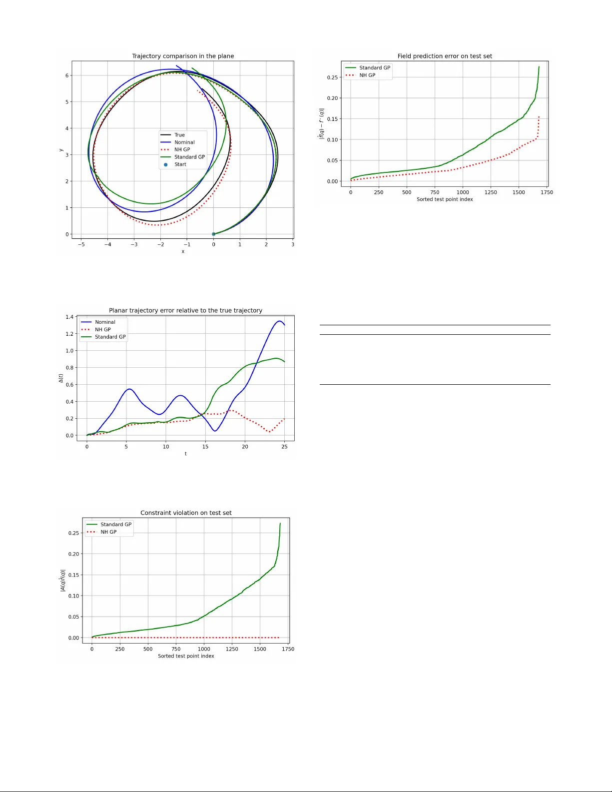
Structur e-Pr eserving Learning of Nonholonomic Dynamics Thomas Beckers, Anthon y Bloch, Leonardo Colombo Abstract — Data-driven modeling is playing an increasing role in robotics and control, yet standard learning methods typically ignore the geometric structur e of nonholonomic systems. As a consequence, the learned dynamics may violate the nonholo- nomic constraints and produce physically inconsistent motions. In this paper , we introduce a structure-preserving Gaussian process (GP) framework for learning nonholonomic dynamics. Our main ingredient is a nonholonomic matrix-valued kernel that incorporates the constraint distrib ution directly into the GP prior . This construction ensures that the learned vector field satisfies the nonholonomic constraints f or all inputs. W e show that the proposed kernel is positive semidefinite, characterize its associated repr oducing ker nel Hilbert space as a space of admissible v ector fields, and pr ove that the resulting estimator admits a coordinate repr esentation adapted to the constraint distribution. W e also establish the consistency of the learned model. Numerical simulations on a vertical rolling disk illustrate the effectiveness of the proposed approach. I . I N T RO D U C T I O N Data-driv en modeling has become an increasingly impor- tant tool in robotics, control, and dynamical systems. In many applications, the dynamics of a system are not perfectly known and must be learned from e xperimental data. Gaussian process (GP) regression has emerged as a powerful nonpara- metric approach for learning unknown dynamics due to its flexibility , probabilistic interpretation, and strong theoretical guarantees [1]. Howe ver , standard machine learning methods typically ignore the geometric structure underlying many mechanical systems. Nonholonomic systems arise frequently in robotics and vehicle dynamics, including wheeled mobile robots and robotic locomotion systems [2], [3], [4]. These systems are characterized by velocity constraints that restrict the admissible directions of motion. As a consequence, their dy- namics e volv e on a distribution of allowable velocities rather than on the full tangent bundle of the configuration space. When learning dynamics directly from data, ignoring these constraints can lead to models that violate the admissible distribution and produce physically inconsistent predictions. Thomas Beckers is with the Department of Computer Science, V anderbilt University , Nashville, TN 37212, USA thomas.beckers@vanderbilt.edu A. Bloch is with Department of Mathematics, Univ ersity of Michigan, Ann Arbor , MI 48109, USA. abloch@umich.edu L. Colombo is with Centre for Automation and Robotics (CSIC-UPM), Ctra. M300 Campo Real, Km 0,200, Arganda del Rey - 28500 Madrid, Spain. leonardo.colombo@csic.es L. Colombo acknowledge financial support from Grant PID2022- 137909NB-C21 funded by MCIN/AEI/ 10.13039/501100011033. The re- search leading to these results was supported in part by iRoboCity2030-CM, Robótica Inteligente para Ciudades Sostenibles (TEC-2024/TEC-62), funded by the Programas de Actividades I+D en T ecnologías en la Comunidad de Madrid. A.Bloch was partially supported by NSF grant DMS-2103026, and AFOSR grants F A 9550-22-1-0215 and F A 9550-23-1-0400. This issue is well kno wn in the modeling of robotic systems, where learned models may generate trajectories that are incompatible with the underlying mechanical constraints. Sev eral works hav e demonstrated that embedding geo- metric structure into learning architectures can markedly improv e the consistency and interpretability of learned dy- namical models. Representativ e examples include Hamilto- nian and Lagrangian neural networks, equiv ariant models on Lie groups, and symmetry-preserving learning methods for Hamiltonian systems with conserved quantities [5], [6], [7], [8], [9], [10], [11], [12]. More recently , nonholonomic learning has started to re- ceiv e attention in approaches based on constraint discovery [13] while nonnholonomic neural netw orks have been exo- plored in [14]. In this work, we incorporate the constraint distribution directly into the Gaussian process prior . In this way , the learned vector field is admissible by construction for every input. In particular , we propose a GP framework for learning nonholonomic dynamics while preserving the constraint distribution. The key idea is to construct a matrix- valued kernel that incorporates the constraint distribution directly into the GP prior . The resulting nonholonomic kernel ensures that the learned vector field automatically satisfies the constraints for all inputs. Main contributions : • W e introduce a nonholonomic kernel that embeds the constraint distribution into the GP prior and we prove that the resulting kernel is positive semidefinite and therefore defines a valid Gaussian process model. • W e characterize the reproducing kernel Hilbert space induced by the kernel and sho w that it consists only of admissible vector fields. • W e establish that learning with the nonholonomic k ernel is equiv alent to Gaussian process regression in coordi- nates adapted to the constraint distribution. • W e prove consistency of the resulting estimator . These results provide a structure-preserving learning framew ork for nonholonomic systems that combines geo- metric modeling with modern machine learning techniques. The paper is structured as follo ws. In Section II, we revie w nonholonomic systems and recall the Gaussian process re- gression frame work used throughout the paper . In Section III, we introduce the nonholonomic kernel and establish its main structural properties and the analysis of the associated estimator , including its coordinate representation adapted to the constraint distribution and consistency properties. In Section IV, we present numerical simulations illustrating the proposed method for the vertical rolling disk. Section V contains concluding remarks and directions for future work. I I . B A C K G RO U N D A. Nonholonomic Mechanics Let Q denote the configuration manifold of a mechanical system, with local coordinates q ∈ Q with dim ( Q ) = n . W e consider nonholonomic systems subject to linear velocity constraints of the form A ( q ) ˙ q = 0 , where A ( q ) ∈ R k × n has full row rank and defines k independent constraints. These constraints define the subspace D q = ker A ( q ) ⊂ T q Q , which specifies the set of allowable velocities at configuration q . A trajectory q ( t ) is admissible if and only if ˙ q ( t ) ∈ D q ( t ) . Thus, the constraints determine a rank- ( n − k ) distribution D ⊂ T Q , whose fiber at each q ∈ Q is D q . For mechanical systems with Lagrangian L ( q , ˙ q ) , the equations of motion subject to the nonholonomic constraints can be written using Lagrange multipliers as λ ∈ R k , see, for instance, [2], [3] d dt ∂ L ∂ ˙ q − ∂ L ∂ q = A ( q ) ⊤ λ, A ( q ) ˙ q = 0 . In this work we focus on learning admissible dynamics of the form ˙ q = f ( q ) , where the v ector field satisfies f ( q ) ∈ D q . T o describe the admissible subspace it is con venient to introduce the orthogonal projector onto the constraint distri- bution. For each q ∈ Q , let P ( q ) = I − A ( q ) † A ( q ) , (1) where A ( q ) † denotes the Moore–Penrose pseudoinv erse. In local coordinates, and with respect to the Euclidean inner product on the ambient coordinate space, P ( q ) is the or- thogonal projector onto the admissible distribution D q = k er A ( q ) . In particular , P ( q ) 2 = P ( q ) and Im( P ( q )) = D q . This representation will be used in the next section to construct Gaussian process kernels that generate vector fields lying in the distribution D . B. Gaussian Processes and Kernels The Gaussian process (GP) provides a nonparametric framew ork for learning unknown functions from data. A GP is fully specified by a mean function m ( q ) and a cov ariance function k ( q, q ′ ) , and is written as f ∼ G P ( m ( q ) , k ( q , q ′ )) . In practice, the mean function is often taken to be zero, which simplifies the resulting expressions without reducing the expressi ve po wer of the model. Thus, in this work we consider the prior f ∼ G P (0 , k ( q, q ′ )) , see [1]. Giv en training inputs q 1 , . . . , q N ∈ Q and corresponding scalar observations y 1 , . . . , y N ∈ R , the kernel matrix (or Gram matrix) is defined by K ij = k ( q i , q j ) , i, j = 1 , . . . , N . Assuming additiv e Gaussian measurement noise with vari- ance σ 2 , the posterior mean prediction at a test point q ∈ Q is given by ˆ f ( q ) = k ( q , Q )  K ( Q, Q ) + σ 2 I  − 1 Y , (2) where Y = [ y 1 , . . . , y N ] ⊤ , K ( Q, Q ) = [ k ( q i , q j )] N i,j =1 is the Gram matrix associated with the training inputs, and k ( q, Q ) = [ k ( q , q 1 ) , . . . , k ( q , q N )] . A symmetric function k : Q × Q → R is called a positive definite kernel if, for any points q 1 , . . . , q N ∈ Q and any coefficients c 1 , . . . , c N ∈ R , N X i,j =1 c i k ( q i , q j ) c j ≥ 0 . This condition guarantees that the associated Gram matrix is positiv e semidefinite and therefore defines a valid cov ariance function for GP regression. For kernels defined on non- Euclidean domains and Riemannian manifolds see [15], [16]. T o learn vector fields on Q , it is natural to consider matrix- valued kernels K : Q × Q → R n × n . Such a kernel is positive semidefinite if, for an y q 1 , . . . , q N ∈ Q and c 1 , . . . , c N ∈ R n , N X i,j =1 c ⊤ i K ( q i , q j ) c j ≥ 0 . Matrix-valued kernels therefore pro vide a natural framew ork for GP models of vector-v alued dynamics [17], [18]. Let Q be a compact set. A continuous positive definite kernel k : Q × Q → R is said to be universal if its associated RKHS H k is dense in C ( Q ) , the space of real-valued continuous functions on Q , with respect to the uniform norm. T ypical examples on compact Euclidean domains include the squared e xponential kernel and suitable Matérn kernels; see, e.g., [19], [20]. I I I . L E A R N I N G N O N H O L O N O M I C D Y N A M I C S A. Nonholonomic Kernel W e now introduce a kernel that incorporates the geometric structure of nonholonomic systems directly into the GP prior . Definition 1: Let k ( q , q ′ ) be a scalar positi ve definite kernel on Q . The nonholonomic kernel associated with the constraint distribution D is defined as K N H ( q , q ′ ) = P ( q ) k ( q, q ′ ) P ( q ′ ) . (3) This kernel produces vector -valued predictions in T Q while enforcing admissibility with respect to the nonholo- nomic constraint distribution D . Definition 2: A reproducing kernel Hilbert space (RKHS) H K associated with a matrix-valued positiv e semidefinite kernel K : Q × Q → R n × n is a Hilbert space of vector- valued functions f : Q → R n such that, for every q ∈ Q and v ∈ R n , the function K ( · , q ) v belongs to H K and the reproducing property ⟨ f , K ( · , q ) v ⟩ H K = ⟨ f ( q ) , v ⟩ R n holds for all f ∈ H K . Associated with the matrix-valued kernel K NH is a RKHS H NH of vector-v alued functions on Q . The following result characterizes H NH and shows that it consists only of vector fields f satisfying f ( q ) ∈ D q for all q ∈ Q . Pr oposition 1: Let H kI n be the RKHS associated with the matrix-v alued kernel K 0 ( q , q ′ ) = k ( q , q ′ ) I n , and define the operator ( T g )( q ) := P ( q ) g ( q ) . Then the RKHS H NH associated with the nonholonomic kernel (3) is gi ven by H NH = { T g : g ∈ H kI n } , endo wed with the norm ∥ f ∥ H NH = inf {∥ g ∥ H kI n : T g = f } . In particular , e very f ∈ H NH can be written as f ( q ) = P ( q ) g ( q ) for some g ∈ H kI n , and hence f ( q ) ∈ D q ∀ q ∈ Q . Pr oof: Define the linear operator T : H kI n → { f : Q → R n } , ( T g )( q ) := P ( q ) g ( q ) . W e claim that the matrix- valued kernel K NH ( q , q ′ ) is precisely the kernel induced by the operator T . Indeed, for any q ′ ∈ Q and c ∈ R n , the kernel section of K 0 is K 0 ( · , q ′ ) c = k ( · , q ′ ) c ∈ H kI n , and applying T gives T  K 0 ( · , q ′ ) P ( q ′ ) c  ( q ) = P ( q ) k ( q , q ′ ) P ( q ′ ) c = K NH ( q , q ′ ) c. Hence every kernel section of K NH belongs to T ( H kI n ) . Con versely , the linear span of such sections is contained in T ( H kI n ) , since for any finite linear combination, N X i =1 K NH ( · , q i ) c i = T N X i =1 K 0 ( · , q i ) P ( q i ) c i ! . Therefore, the RKHS generated by K NH is exactly the image of H kI n under T , endowed with the standard norm ∥ f ∥ H NH = inf {∥ g ∥ H kI n : T g = f } . It follo ws that ev ery f ∈ H NH admits a representation f = T g with g ∈ H kI n , that is, f ( q ) = P ( q ) g ( q ) . Since Im( P ( q )) = D q , then f ( q ) ∈ D q , ∀ q ∈ Q . Remark 1: The previous proposition shows that the non- holonomic kernel does not merely project the posterior prediction a posteriori. Rather , it restricts the entire GP prior to vector fields taking values in D . Pr oposition 2: If k ( q , q ′ ) is positiv e definite, then the nonholonomic kernel K N H ( q , q ′ ) is a positive semidefinite matrix-valued kernel. Pr oof: Let c 1 , . . . , c N ∈ R n be arbitrary vectors. Then N X i,j =1 c T i K N H ( q i , q j ) c j = N X i,j =1 c T i P ( q i ) k ( q i , q j ) P ( q j ) c j . Defining ˜ c i = P ( q i ) c i giv es N X i,j =1 ˜ c T i k ( q i , q j )˜ c j ≥ 0 , since k is positive definite. Propositions 1 and 2 together show that the proposed non- holonomic kernel defines a valid GP model whose associated hypothesis space consists only of admissible vector fields. W e now make this implication explicit at the lev el of the GP predictor , sho wing that the posterior mean automatically satisfies the nonholonomic constraints for ev ery input. Pr oposition 3: Let ˆ f ( q ) be the Gaussian process predic- tor obtained using the nonholonomic kernel K N H . Then A ( q ) ˆ f ( q ) = 0 for all q ∈ Q . Pr oof: From the definition of the nonholonomic kernel, any mean function generated by the Gaussian process has the form ˆ f ( q ) = N X i =1 K N H ( q , q i ) c i . Substituting the kernel definition gives ˆ f ( q ) = P ( q ) N X i =1 k ( q, q i ) P ( q i ) c i . Since P ( q ) is the orthogonal projector onto D q , we hav e A ( q ) P ( q ) = 0 . Therefore A ( q ) ˆ f ( q ) = 0 . B. Adapted Coordinates Interpr etation Nonholonomic systems admit a natural representation in terms of coordinates adapted to the constraint distribution. Let B ( q ) ∈ R n × ( n − k ) be a smooth matrix whose columns form a basis of the D q , i.e., D q = Im( B ( q )) . Any admissible v elocity can then be written as ˙ q = B ( q ) ν , where ν ∈ R n − k represents the generalized velocity in adapted coordinates to D . Consequently , any admissible vec- tor field f ( q ) satisfying f ( q ) ∈ D q admits the representation f ( q ) = B ( q ) ν ( q ) , (4) for some vector field ν ( q ) adapted to D . Next, we show that the nonholonomic kernel implicitly performs GP regression on these adapted coordinates. Theor em 1: Let B ( q ) ∈ R n × ( n − k ) be a smooth matrix whose columns form a basis of the constraint distribution D q , so that D q = Im( B ( q )) . Then every function f ∈ H NH admits a representation f ( q ) = B ( q ) ν ( q ) , for some v ector field ν ( q ) on D . Accordingly , learning with the nonholo- nomic kernel admits an equiv alent representation in adapted coordinates to the constraint distribution. Pr oof: Any function f ∈ H NH can be written as f ( q ) = P ( q ) g ( q ) , for some vector -valued function g . Since P ( q ) projects onto D q and D q = Im( B ( q )) , there e xists a pseudoin verse B ( q ) † such that P ( q ) = B ( q ) B ( q ) † . There- fore f ( q ) = B ( q ) B ( q ) † g ( q ) . Defining ν ( q ) = B ( q ) † g ( q ) , we obtain f ( q ) = B ( q ) ν ( q ) . Thus ev ery admissible function generated by the nonholo- nomic kernel can be represented in adapted coordinates. Remark 2: The previous theorem should be understood as a representation result at the lev el of admissible function classes. An exact statistical equiv alence between regression in ambient coordinates and regression in adapted coordinates additionally depends on the observation model and on how measurement noise transforms under the map B ( q ) † . Remark 3: Theorem 1 provides an alternativ e interpreta- tion of the proposed method. Instead of explicitly parame- terizing the admissible dynamics using adapted coordinates B ( q ) , the nonholonomic kernel enforces the same structure implicitly through the projection operator P ( q ) . As a conse- quence, the Gaussian process prior is automatically restricted to vector fields compatible with the constraint distribution. C. Consistency of the Estimator W e no w study the statistical properties of the estimator induced by the nonholonomic kernel. In particular , we show that the resulting GP scheme is consistent for the true admissible vector field, provided that the latter belongs to, or is well approximated by , the function class induced by the underlying scalar kernel. Assume that we observe noisy samples of the vector field y i = f ⋆ ( q i ) + ε i , where q i ∈ Q , the noise terms ε i are independent Gaussian variables with v ariance σ 2 , and the true dynamics f ⋆ satisfy the nonholonomic constraints f ⋆ ( q ) ∈ D q . Let ˆ f N denote the GP estimator obtained from N samples using the nonholonomic kernel K N H . Pr oposition 4: Let ˆ g N denote an estimator obtained with the kernel k ( q , q ′ ) I n , and let ˆ f N be the estimator induced by the nonholonomic kernel, so that ˆ f N ( q ) = P ( q ) ˆ g N ( q ) . Assume that the true admissible dynamics satisfy f ⋆ ( q ) = P ( q ) g ⋆ ( q ) for some vector-v alued function g ⋆ . Then ∥ ˆ f N ( q ) − f ⋆ ( q ) ∥ ≤ ∥ P ( q ) ∥ ∥ ˆ g N ( q ) − g ⋆ ( q ) ∥ . (5) Pr oof: From the construction of the estimator we hav e ˆ f N ( q ) = P ( q ) ˆ g N ( q ) , and f ⋆ ( q ) = P ( q ) g ⋆ ( q ) . Therefore ˆ f N ( q ) − f ⋆ ( q ) = P ( q )( ˆ g N ( q ) − g ⋆ ( q )) . T aking norms, ∥ ˆ f N ( q ) − f ⋆ ( q ) ∥ ≤ ∥ P ( q ) ∥ ∥ ˆ g N ( q ) − g ⋆ ( q ) ∥ . Remark 4: Proposition 4 shows that the projection step is stable: the error of the nonholonomic estimator is con- trolled by the error of the underlying unconstrained estimator through the operator norm of P ( q ) . Since P ( q ) is an orthog- onal projector, one has ∥ P ( q ) ∥ ≤ 1 in the induced Euclidean operator norm. Hence ∥ ˆ f N ( q ) − f ⋆ ( q ) ∥ ≤ ∥ ˆ g N ( q ) − g ⋆ ( q ) ∥ . Next, we address the uni versal propery of the proposed nonholonomic kernel. Let Q be a compact set. A continuous positiv e definite kernel k : Q × Q → R is said to be universal if its associated RKHS H k is dense in C ( Q ) , the space of real-v alued continuous functions on Q , with respect to the uniform norm. T ypical examples on compact Euclidean domains include the squared e xponential kernel and suitable Matérn kernels; see, e.g., [19], [20]. Assumption 1: The scalar kernel k ( q , q ′ ) is uni versal on the compact set Q . Assumption 2: The true vector field f ⋆ belongs to the RKHS H N H associated with the nonholonomic kernel. Assumption 2 is a standard realizability assumption in RKHS-based consistency analysis. It requires that the true admissible dynamics lie in the space induced by the nonholo- nomic kernel, i.e., they can be represented as the projection of a suf ficiently regular ambient v ector field. While this is not automatic, it is natural for smooth nonholonomic dynamics on compact domains and for sufficiently rich scalar kernels. Theor em 2: Let ˆ f N be the Gaussian process estimator obtained using the nonholonomic kernel K NH and N dis- tinct training samples. Under the above assumptions, ˆ f N is uniformly consistent in probability , namely , for ev ery ε > 0 , P  sup q ∈ Q ∥ ˆ f N ( q ) − f ⋆ ( q ) ∥ > ε  → 0 as N → ∞ . Pr oof: By Proposition 1, the RKHS associated with the nonholonomic kernel is H NH = { f : Q → R n | f ( q ) = P ( q ) g ( q ) , g ∈ H kI n } . Since f ⋆ ∈ H NH , there exists g ⋆ ∈ H kI n such that f ⋆ ( q ) = P ( q ) g ⋆ ( q ) , q ∈ Q . Let ˆ g N denote the Gaussian process estimator associated with the kernel K 0 ( q , q ′ ) = k ( q, q ′ ) I n . Under Assumptions 1 and 2 and standard consistency results for kernel-based GP regression, ˆ g N is uniformly consistent in probability for g ⋆ , namely , for ev ery ε > 0 , P  sup q ∈ Q ∥ ˆ g N ( q ) − g ⋆ ( q ) ∥ > ε  → 0 as N → ∞ . On the other hand, the estimator induced by the nonholo- nomic kernel satisfies ˆ f N ( q ) = P ( q )ˆ g N ( q ) . Therefore, for ev ery q ∈ Q , ˆ f N ( q ) − f ⋆ ( q ) = P ( q )  ˆ g N ( q ) − g ⋆ ( q )  , and hence ∥ ˆ f N ( q ) − f ⋆ ( q ) ∥ ≤ ∥ P ( q ) ∥ ∥ ˆ g N ( q ) − g ⋆ ( q ) ∥ . By construction, P ( q ) = I − A ( q ) † A ( q ) is the orthogonal projector onto D q = k er A ( q ) . In particular, P ( q ) is self- adjoint and idempotent, that is, P ( q ) ⊤ = P ( q ) and P ( q ) 2 = P ( q ) . Hence, with respect to the Euclidean norm, its operator norm satisfies ∥ P ( q ) ∥ ≤ 1 , q ∈ Q . Indeed, if v ∈ R n is decomposed orthogonally as v = v D + v D ⊥ , v D ∈ D q , v D ⊥ ∈ D ⊥ q , then P ( q ) v = v D , and therefore ∥ P ( q ) v ∥ = ∥ v D ∥ ≤ ∥ v ∥ . Consequently , sup q ∈ Q ∥ ˆ f N ( q ) − f ⋆ ( q ) ∥ ≤ sup q ∈ Q ∥ ˆ g N ( q ) − g ⋆ ( q ) ∥ . Now let ε > 0 . Then P  sup q ∈ Q ∥ ˆ f N ( q ) − f ⋆ ( q ) ∥ > ε  ≤ P  sup q ∈ Q ∥ ˆ g N ( q ) − g ⋆ ( q ) ∥ > ε  . Since the right-hand side conv erges to zero as N → ∞ , we conclude that, for ev ery ε > 0 , P  sup q ∈ Q ∥ ˆ f N ( q ) − f ⋆ ( q ) ∥ ε  → 0 as N → ∞ . This estimate shows that consistency of the unconstrained estimator ˆ g N transfers directly to the projected estimator ˆ f N , provided the target dynamics admit the representation f ⋆ ( q ) = P ( q ) g ⋆ ( q ) . Hence, the nonholonomic construction preserves the approximation properties of the underlying regression method while enforcing the constraints exactly . I V . N U M E R I C A L E X A M P L E : V E RT I C A L RO L L I N G D I S K T o illustrate the proposed nonholonomic Gaussian process framew ork, we consider the vertical rolling disk, see [2]. The configuration space is Q = S E (2) × S 1 ∼ = R 2 × S 1 × S 1 with coordinates q = ( x, y , φ, θ ) , where ( x, y ) denotes the contact point on the plane, φ is the orientation of the disk in the plane, and θ is the rotation angle of the disk. The rolling-without-slipping constraints are ˙ x − R cos φ ˙ θ = 0 , ˙ y − R sin φ ˙ θ = 0 . (6) These define the constraint distribution with constraint matrix A ( q ) =  1 0 0 − R cos φ 0 1 0 − R sin φ  . (7) A con venient basis of the distribution is giv en by the vector fields X 1 ( q ) =  R cos φ R sin φ 0 1  T and X 2 ( q ) =  0 0 1 0  T , so that ev ery admissible velocity can be written as ˙ q = B ( q ) ν, B ( q ) =  X 1 ( q ) X 2 ( q )  , ν ∈ R 2 . By construction, A ( q ) B ( q ) = 0 . W e consider admissible dynamics of the form ˙ q = f ( q ) , with f ( q ) ∈ D q . Rather than learning arbitrary vector fields in the ambient tangent bundle, we work with dynamics that are admissible through the representation f ( q ) = B ( q ) ν ( q ) , where ν ( q ) ∈ R 2 is an adapted velocity field to D . W e define a nominal model f nom ( q ) = B ( q ) ν nom ( q ) , and the perturbed dynamics f ⋆ ( q ) = B ( q ) ν ⋆ ( q ) , ν ⋆ ( q ) = ν nom ( q ) + δ ( q ) , where δ ( q ) is a smooth model disturbance. Thus, the true dy- namics is obtained by augmenting the nominal field adapted to D with an unmodeled component, while admissibility is preserved by construction. Because both vector fields are generated through the same distribution basis B ( q ) , they satisfy f nom ( q ) , f ⋆ ( q ) ∈ D q for all q ∈ Q , so admissibility is preserved by construction. In the simulation we use the parameters R = 1 , Ω = 1 . 0 , ω = 0 . 35 , ε = 0 . 18 , where Ω and ω denote the nominal (baseline) angular rates of the dynamics on adapted coordinates, and ε sets the amplitude of the perturbation. T o av oid an ov erly degenerate nominal trajectory , the nominal velocity field ν nom is chosen to be weakly state-dependent, rather than constant: ν nom ( q ) = " Ω + 0 . 10 sin φ + 0 . 06 cos θ ω + 0 . 08 cos φ − 0 . 05 sin θ # . The true v elocity field is then defined by adding the smooth perturbation δ ( q ) = ε " 0 . 60 sin( φ − θ ) + 0 . 25 cos(2 θ ) 0 . 50 cos( φ + θ ) − 0 . 20 sin(2 φ ) # , so that ν ⋆ ( q ) = ν nom ( q ) + δ ( q ) , and therefore f ⋆ ( q ) = B ( q ) ν ⋆ ( q ) satisfies f ⋆ ( q ) ∈ D q for all q ∈ Q . T raining data are generated from the true model by sam- pling states along three true trajectories with initial condi- tions (0 , 0 , 0 . 2 , 0 . 1) , (0 , 0 , − 0 . 6 , 0 . 4) and (0 , 0 , 0 . 8 , − 0 . 5) , integrated with time step ∆ t = 0 . 05 . The sampled states are then subsampled to obtain N train = 120 training points. Gaussian perturbations with standard de viation σ state = 0 . 05 are added to the angular coordinates ( φ, θ ) of the sampled states, and noisy observations are generated as y i = f ⋆ ( q i ) + η i , η i ∼ N (0 , σ 2 I ) , with σ = 0 . 03 . The horizon time for testing is chosen as T = 25 . W e compare two Gaussian process models. The first is a standard vector-v alued Gaussian process with kernel K std ( q , q ′ ) = k ( q , q ′ ) I 4 , which does not encode the non- holonomic constraints. The second is the proposed Gaus- sian process with the nonholonomic kernel K NH ( q , q ′ ) = P ( q ) k ( q, q ′ ) P ( q ′ ) , whose posterior mean predictor is de- noted by ˆ f NH , where P ( q ) = I − A ( q ) † A ( q ) is the orthog- onal projector onto D . In this example, since R = 1 , the basis matrix is B ( q ) =  (cos φ, sin φ, 0 , 1) T , (0 , 0 , 1 , 0) T  and the projector can be written explicitly as P ( q ) = B ( q )  B ( q ) ⊤ B ( q )  − 1 B ( q ) ⊤ , that is, P ( q ) =     cos 2 φ 2 sin φ cos φ 2 0 cos φ 2 sin φ cos φ 2 sin 2 φ 2 0 sin φ 2 0 0 1 0 cos φ 2 sin φ 2 0 1 2     . (8) By the results established in Section III, the nonholonomic kernel restricts the entire GP prior to admissible vector fields and therefore guarantees A ( q ) ˆ f NH ( q ) = 0 , for all q ∈ Q . In all experiments we use a squared-exponential scalar kernel acting on the angular variables ( φ, θ ) , k ( q, q ′ ) = σ 2 f exp − 1 2  φ − φ ′ θ − θ ′  ⊤ Λ − 1  φ − φ ′ θ − θ ′  ! , (9) with Λ = diag( ℓ 2 φ , ℓ 2 θ ) . Here σ 2 f denotes the signal variance, ( ℓ φ , ℓ θ ) the length scales, and σ 2 n the noise variance. The standard GP is trained directly in ambient coordinates R 4 , whereas the nonholonomic GP is trained in the adapted co- ordinates ν ∈ R 2 and mapped back to ambient space through B ( q ) . The kernel hyperparameters obtained by marginal likelihood optimization are summarized in T able I. In this Model / channel σ 2 f ℓ φ ℓ θ σ 2 n Stand. GP , outp 1 0 . 949 2 1.50 2.18 0.00198 Stand. GP , output 2 1 . 49 2 1.50 2.46 0.00409 Stand. GP , output 3 1 . 21 2 1.27 1.70 0.0939 Stand. GP , output 4 0 . 989 2 1.39 1.28 0.0583 NH GP , adapted 1 1 . 02 2 1.47 1.35 0.0306 NH GP , adapted 2 1 . 21 2 1.27 1.70 0.0939 T ABLE I: Standard vs. nonholonomic GP example the squared-exponential kernel is implemented in the angular chart ( φ, θ ) . Since the trajectories considered here remain in a regime where this chart representation is numerically adequate, we use the corresponding Euclidean RBF kernel. A more intrinsic treatment on S 1 × S 1 could alternativ ely employ periodic kernels, see [1]. T o assess model quality , we compare both local vector - field prediction and trajectory-lev el performance. First, we ev aluate the pointwise prediction error e f ( q ) = ∥ ˆ f ( q ) − f ⋆ ( q ) ∥ . Second, we measure violation of the nonholonomic constraints through e nh ( q ) = ∥ A ( q ) ˆ f ( q ) ∥ . For the nonholo- nomic GP , this quantity v anishes identically up to numerical precision, whereas for the unconstrained GP it is generally nonzero. Third, we inte grate the learned vector fields and compare the resulting trajectories with the true trajectory . If q ⋆ ( t ) denotes the trajectory generated by f ⋆ and ˆ q ( t ) the trajectory generated by a learned model, we use the planar tracking error as a physical observable: ∆( t ) = p ( x ⋆ ( t ) − ˆ x ( t )) 2 + ( y ⋆ ( t ) − ˆ y ( t )) 2 . (10) Fig. 1 displays the resulting trajectories. The nominal model exhibits a visible drift with respect to the true trajec- tory . The unconstrained GP already improves the prediction substantially , but the proposed nonholonomic GP yields the closest trajectory to the ground truth over the full horizon time. This is confirmed quantitatively in Fig. 2, which reports the planar trajectory error ∆( t ) . The nonholonomic GP achiev es the smallest error over essentially the entire simulation interval and improv es upon both the nominal model and the unconstrained GP . Fig. 3 shows the constraint violation metric e nh ( q ) = ∥ A ( q ) ˆ f ( q ) ∥ ov er the test set. As predicted by the theory , the nonholonomic GP preserves the rolling constraints exactly up to numerical precision, while the unconstrained GP produces nonzero components outside the admissible distribution. Fi- nally , Fig. 4 reports the pointwise field prediction error e f ( q ) = ∥ ˆ f ( q ) − f ⋆ ( q ) ∥ on the test set. The nonholonomic GP also provides the smallest field error , sho wing that its geometric consistency does not come at the expense of predictiv e accuracy . On the contrary , in this example the nonholonomic prior impro ves both local field approximation and long-horizon trajectory prediction. Fig. 1: Trajectory comparison in the plane: true dynamics, nominal model, nonholonomic GP , and standard GP . Fig. 2: Planar trajectory error ∆( t ) for the nominal, nonholo- nomic GP , and standard GP models. Fig. 3: Constraint violation metric e nh ( q ) = ∥ A ( q ) ˆ f ( q ) ∥ for the standard and nonholonomic GP models. Fig. 4: Pointwise field prediction error e f ( q ) = ∥ ˆ f ( q ) − f ⋆ ( q ) ∥ on the test set. T able II sho ws the numerical results. The nonholonomic GP achie ves the smallest mean field error , exactly preserves the constraint distribution, and yields the lowest mean and final trajectory errors among all models considered. Metric Nominal Standard GP NH GP Mean field err . — 0.067409 0.035205 Mean constr . viol. — 5 . 873109 × 10 − 2 0 Max constr . viol. — 2 . 722539 × 10 − 1 0 Mean planar err . 0.449343 0.373659 0.148855 Final planar err . 1.302615 0.868002 0.194430 T ABLE II: Metrics used for the vertical rolling disk. V . C O N C L U S I O N S A N D F U T U R E W O R K W e introduced a nonholonomic kernel for GP regres- sion that enforces the nonholonomic constraints exactly by projecting a scalar kernel onto the constraint distribution. The resulting construction yields valid vector-v alued kernels, restricts the associated RKHS to admissible vector fields, and preserves consistency of the underlying regression scheme. Future work will address learning on reduced nonholo- nomic systems, where the reconstruction process can make the estimation problem substantially more challenging. W e also plan to incorporate volume variation as an additional metric in examples such as the Chaplygin sleigh and the Suslov problem, where volume is not necessarily preserved and may play an important role in the learning behavior . R E F E R E N C E S [1] C. E. Rasmussen and C. K. Williams, Gaussian pr ocesses for machine learning . MIT press Cambridge, 2006, vol. 1. [2] A. M. Bloch, “Nonholonomic mechanics, ” in Nonholonomic mechan- ics and control . Springer , 2003. [3] J. Cortés, Geometric, contr ol and numerical aspects of nonholonomic systems . Springer Science & Business Media, 2002, no. 1793. [4] J. I. Neimark and N. A. Fufae v , Dynamics of nonholonomic systems . American Mathematical Soc., 2004, vol. 33. [5] S. Greydanus, M. Dzamba, and J. Y osinski, “Hamiltonian neural networks, ” in Advances in Neural Information Pr ocessing Systems , vol. 32, 2019. [6] P . Jin, Z. Zhang, A. Zhu, Y . T ang, and G. E. Karniadakis, “Symp- nets: Intrinsic structure-preserving symplectic networks for identifying hamiltonian systems, ” Neural Networks , vol. 132, pp. 166–179, 2020. [7] Y . D. Zhong, B. Dey , and A. Chakraborty , “Symplectic ode-net: Learn- ing hamiltonian dynamics with control, ” in International Conference on Learning Representations , 2020. [8] M. Cranmer , S. Greydanus, S. Hoyer , P . Battaglia, D. Spergel, and S. Ho, “Lagrangian neural networks, ” in ICLR 2020 W orkshop on Inte gration of Deep Neural Models and Differ ential Equations . [9] M. Finzi, S. Stanton, P . Izmailo v , and A. G. W ilson, “Generalizing con- volutional neural networks for equivariance to lie groups on arbitrary continuous data, ” in Proceedings of the 37th International Confer ence on Machine Learning , ser . Proceedings of Machine Learning Research, vol. 119. PMLR, 2020, pp. 3165–3176. [10] M. V aquero, J. Cortés, and D. M. de Die go, “Symmetry preservation in hamiltonian systems: Simulation and learning, ” Journal of Nonlinear Science , vol. 34, no. 6, p. 115, 2024. [11] C. Eldred, F . Gay-Balmaz, S. Huraka, and V . Putkaradze, “Lie–poisson neural networks (lpnets): Data-based computing of hamiltonian sys- tems with symmetries, ” Neural Networks , vol. 173, p. 106162, 2024. [12] T . Beckers, J. Seidman, P . Perdikaris, and G. J. Pappas, “Gaussian process port-hamiltonian systems: Bayesian learning with physics prior , ” in 2022 IEEE 61st Conference on Decision and Control (CDC) . IEEE, 2022, pp. 1447–1453. [13] B. W ang and A. Bloch, “Learning nonholonomic dynamics with constraint discov ery , ” arXiv preprint , 2024. [14] V . A. Díaz, L. M. Salomone, and M. Zuccalli, “Lagrangian neural networks for nonholonomic mechanics, ” Chaos, Solitons & F ractals , vol. 199, p. 116867, 2025. [15] S. Jayasumana, R. Hartley , M. Salzmann, H. Li, and M. Harandi, “Ker - nel methods on riemannian manifolds with gaussian RBF kernels, ” IEEE T ransactions on P attern Analysis and Machine Intelligence , vol. 37, no. 12, pp. 2464–2477, 2015. [16] V . Borovitskiy , A. T erenin, P . Mosto wsky , and M. P . Deisenroth, “Matérn gaussian processes on riemannian manifolds, ” in Advances in Neural Information Pr ocessing Systems , vol. 33, 2020, pp. 12 426– 12 437. [17] C. A. Micchelli and M. Pontil, “On learning vector-v alued functions, ” Neural computation , vol. 17, no. 1, pp. 177–204, 2005. [18] C. Carmeli, E. De V ito, A. T oigo, and V . Umanitá, “V ector valued reproducing kernel hilbert spaces and univ ersality , ” Analysis and Applications , vol. 8, no. 01, pp. 19–61, 2010. [19] I. Steinwart and A. Christmann, Support vector machines . Springer Science & Business Media, 2008. [20] B. K. Sriperumbudur , K. Fukumizu, A. Gretton, B. Schölkopf, and G. R. G. Lanckriet, “Uni versality , characteristic kernels and rkhs embedding of measures, ” Journal of Machine Learning Researc h , vol. 12, pp. 2389–2410, 2011.