MPC-Based Trajectory Tracking for a Quadrotor UAV with Uniform Semi-Global Asymptotic Stability Guarantees

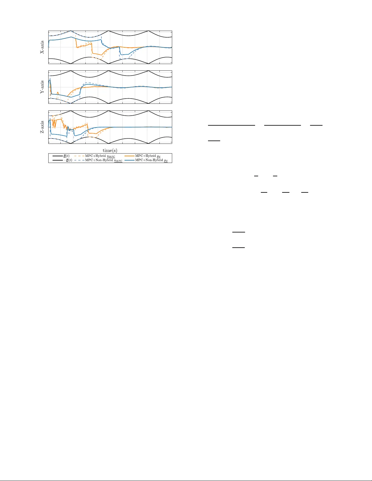
MPC-Based T rajectory T racking f or a Quadr otor U A V with Unif orm Semi-Global Asymptotic Stability Guarantees Qian Y ang, Miaomiao W a ng, Abdelhamid T aye bi Abstract — This paper proposes a model predictive trajectory tracking approach fo r quadrotors sub ject to input constraints. Our proposed approach relies on a hierarchical contro l strategy with an outer -loop feedback generating the required thrust and desired attitude and an inner -loop feedback regulating the actual attitude to the desired one. For th e outer -loop translational dynamics, the generation of the virtual control input is fo rmulated as a constrained model predictiv e contr ol problem with ti me-va rying input constraint s and a contro l strategy , endowed with uniform global asymptotic stability guarantees, is proposed. F or the inner -loop rotational dynamics, a hybrid geometric controller is adopted achieving semi-global exponential tracking of the desired attitude. Finally , we prov e that the ov erall cascaded system is semi-globally asymptotically stable. Simulation results illu strate th e effectiv eness of the proposed approach. I . I N T R O D U C T I O N Quadroto rs are versatile u nmanne d aerial vehicles (U A Vs) used in many ind u strial and hobby app lica tio ns, due to their high man euverability an d vertical takeoff and lan ding capability . Due to the un d eractuated natu re of these systems, the hierarch ical inner-outer loo p con trol p aradigm is a com- monly adopted solution f or the trajecto ry tracking problem for quadro tor U A Vs. The ou te r-loop feed back dea ls with the translational dynamics wh ere a v irtual co ntrol input is designed to regulate the quadroto r’ s po sition to th e d esired one. The thrust input and the desired or ie n tation a r e then extracted from th is vir tual inpu t and th e inner loop takes care of regulating the actual orientation to the desired one (see, for instan ce, [1 ]–[3]) . V arious attitude co ntrol tech- niques have b een developed in th e literature using different attitude rep resentations such as the unit-q uaternion [4], [ 5] and the special o rthogon al group SO(3) [6]. Due to the topolog ical obstru ction o n SO(3 ) , continu ous tim e -in variant feedback ca nnot ach iev e glob al asympto tic stability (GAS) on SO (3) [7 ]. T o overcome this limitation, hybr id feed back control tec hniques, e n dowed with glo bal asy m ptotic stability guaran tee s, h av e been pro posed in the literatu re [8] –[10] . In prac tical applications, the tr ajectory trac king of qu adro- tor U A Vs must take into consideration practical requir ements such as actuator satura tions. Existing meth ods usually gu ar- antee these requiremen ts by restricting th e oute r-loop contro l This wo rk was supporte d in part by the National Natural Science Founda tion of China under Grant 62403205, and in part by the Na- tional Scien ces and Engineer ing Research Council of Canada under Grant NSERC-DG RGPIN-2020-06270. Q. Y ang and M. W ang are with the S chool of Artificial Intellige nce and Automation, Huazhong Uni versit y of Scienc e a nd T echn ology , W uhan 430074, China (e-mail: mmwang@hust.e du.cn ). A. T ayebi i s wi th the Departmen t of Elec tri- cal E nginee ring, Lak ehead U nive rsity , Thunder Bay , ON P7B 5E1, Cana da (e-mail: a tayebi@lakehead u.ca ). parameters. Mo del pr edictiv e contro l (MPC) is an attractive approa c h when it comes to handling inp u t constra in ts. In [11], MPC was employed for the o u ter-loop feedba ck d esign for a q uadroto r U A V . The tr a nslational dynamics was dy- namically extend ed to generate a twice- differentiable desired attitude to be used by the inner-loop controller . T o ensure that the actual virtual inp u t satisfies the prescribe d time-varying constraint, a unifo r m conservati ve constraint was imp osed on the augm ented virtual input in the MPC form ulation. T o relax the conservativ e con straints co nditions in [11 ], th e authors in [12] sugge sted to up date the time-varying con stra int at each sampling in stan t. Both appr oaches in [11] , [12] achieve unifor m alm o st glob al asym ptotic stability (U A GAS) of the overall closed- loop system. H owever , neither approach allows the original time-v aryin g constraint to be imposed directly on th e augm ented virtua l in p ut. In this pap er , we propose a hierar chical c ontrol framework for quadro tor trajector y tracking . In the ou te r-loop , an MPC strategy is designe d to achiev e UGAS in the continuo us- time sense. In particular, b ased on [11] , a scale factor is introdu c ed so that the o riginal time-varying constraints can be applied directly to the aug mented virtual input in the MPC formu lation. For th e inner-loop, a hybrid attitude con- troller is adopted to ensure semi-glo b al expon ential stability (SGES). Uniform semi-global asymptotic stab ility (USGAS) of the overall ca scad ed closed -loop system is rigor o usly established. I I . P R E L I M I NA R I E S A. Notation a nd Definitio n s Denote the sets of all real nu mbers an d non-n egati ve integers by R and N , resp e cti vely . W e deno te by R n the n -dimensio n al Euclidean space, and d e note b y I n and 0 m × n the n -b y - n identity matrix and the m -by- n matr ix with all zero elements, respectively . Let e 1 , e 2 , e 3 ∈ R 3 denote the standard basis vectors. Define the 2-no r m of vector a ∈ R n as k a k , and the ind uced 2- n orm of matrix A ∈ R m × n as k A k 2 . For some symmetr ic matrix P = P ⊤ ≻ 0 , we d efine k x k 2 P = x ⊤ P x for a vector x ∈ R n . Moreover , let | x | A denote the distance of a point x ∈ M to a closed set A ⊂ M . W e write λ max ( P ) ( λ min ( P ) ) for the m a x imum (minimum ) eigenvalue of P . For any vector p ∈ R n , we denote by p i the i th compo nent of p . For any vector x = [ x 1 , x 2 , x 3 ] ⊤ ∈ R 3 , we define ( · ) × as a ske w- symmetric operator given by x × = [0 , − x 3 , x 2 ; x 3 , 0 , − x 1 ; − x 2 , x 1 , 0] , such that for any x, y ∈ R 3 , the id entity x × y = x × y holds, whe r e × denotes the vector cross pr oduct operato r , and vec( · ) as the in verse opera to r of the ma p ( · ) × , such that v ec( x × ) = x . In addition, vec ( · ) : R m × n → R mn denotes the column- stacking operator, which maps a matrix to a vector by concaten ating its columns in o rder . Let SO(3) denote the special ortho gonal g roup of order three, i.e. , S O (3) = { R ∈ R 3 × 3 | R R ⊤ = R ⊤ R = I 3 , det( R ) = 1 } . W e defin e the saturation fun c tio n σ ∆ : R → R , for a giv en ∆ > 0 , such that 1) | σ ∆ ( x ) | ≤ ∆ ∀ x ∈ R ; 2) xσ ∆ ( x ) > 0 ∀ x 6 = 0 , σ ∆ (0) = 0 ; 3) σ ∆ is differentiable, and 0 < dσ ∆ ( x ) dx ≤ 1 ; 4) The deriv ativ e σ ′ ∆ ( x ) = dσ ∆ ( x ) dx is nonincrea sin g o n (0 , + ∞ ) and non decreasing o n ( −∞ , 0) . Denote Ψ ∆ ( x ) = R x 0 σ ∆ ( s ) ds . The fo llowing lem ma on the saturation fu nction will be u sed throug hout this pape r . Lemma 1: For all a > 0 , b ∈ [0 , 1] , and x ∈ R , the following inequality h o lds: 1) σ ∆ ( ax ) f ( x ) ≤ axf ( x ) , wher e f : R → R satisfies xf ( x ) > 0 , ∀ x 6 = 0 and f (0) = 0 ; 2) bxσ ∆ ( x ) ≤ xσ ∆ ( bx ) ; 3) Ψ ∆ ( x ) ≤ xσ ∆ ( x ) . Pr oo f: See Ap pendix A I I I . P R O B L E M F O R M U L A T I O N Let R ∈ SO (3 ) den ote the attitud e of the body -fixed fram e with respect to th e inertial fram e , an d ω ∈ R 3 denote the body- fixed fram e a n gular velocity . L et p, v ∈ R 3 denote the position and line a r velocity expressed in the inertial frame, respectively . The d ynamics model of a U A V is given by ˙ p = v (1a) ˙ v = g e 3 − T Re 3 − Dv (1b) ˙ R = Rω × (1c) J ˙ ω = − ω × J ω + τ (1d) where g is the acceleration of gravity , T d enotes the thrust normalized by ma ss, D = diag( d 1 , d 2 , d 3 ) , d 1 , d 2 , d 3 > 0 , are the mass-n o rmalized rotor dr a g coefficients, J = J ⊤ ∈ R 3 × 3 is th e constant in ertia m atrix, and τ ∈ R 3 is the contro l torque in put. The thrust is con sidered to be nonnegative and limited acco rding to 0 ≤ T ( t ) ≤ T max for all t ≥ 0 , where T max > g is the maximal thrust. This model is adapted from [11]. Compa r ed with the model in [1 1], ( 1d ) is written in a mo r e standar d f orm. Th is difference does n ot materially affect th e sub sequent contr o ller design, since the additional terms in the reference d models can be absorbed into the feedfor ward term. Consider a con tinuous time-varying ref erence trajector y r ( t ) ∈ R 3 . Giv en the m odel in ( 1 ), the objective is to design T and τ so that the system tracks a given contin uous r efer- ence r ( t ) . T o achieve the objec ti ve, we m ake the fo llowing mild assump tion. Assumption 1: Suppose r ( t ) is f o ur times d ifferentiab le, and its first four deriv atives ˙ r ( t ) , ¨ r ( t ) , r (3) ( t ) , and r (4) are unifor m ly b ounded with k nown b ounds. I n addition, ther e exist p ositi ve co nstants δ r and δ r z satisfying k D ˙ r + ¨ r k ≤ δ r < T max − g a n d e ⊤ 3 ( D ˙ r + ¨ r ) < δ r z < g . Defining the error state as ˜ p = p − r, ˜ v = v − ˙ r , th e error dynamics are g i ven by ˙ ˜ p = ˜ v (2a) ˙ ˜ v = g e 3 − T Re 3 − Dv − ¨ r = g e 3 − T Re 3 − ¨ r − D ˙ r − D ˜ v := µ − D ˜ v (2b) with µ = g e 3 − T Re 3 − ¨ r − D ˙ r. The variable µ is v ie wed a s a virtu al control inp ut for the translational error dynam ics. By app ropriately designing µ , both ˜ p and ˜ v can b e regulated to zero. Define µ d as th e desired v irtual inp ut given b y µ d = g e 3 − T R d e 3 − ¨ r − D ˙ r (3) where R d denotes the desired a ttitude to be tracked by tracked by the actual attitude R v ia the control torque τ . Equation ( 3 ) determ in es only th e third column of R d , so the extraction of R d from µ d is intrin sically nonun ique. Furthermo re, the extraction map is sing ular on a non e mpty set. Hence, b esides the physical constraints induced by T max , ˙ r , and ¨ r , the desired v irtual inpu t µ d must satisfy an additional adm issibility condition to guara ntee a well-d efined extraction o f R d . The correspon ding boun d is den o ted b y B ( ˙ r , ¨ r ) , who se explicit form will be given in a later section of the p aper . Moreover , the implem entation of a geometric controller such as that in [1 3] to drive R tow ard R d requires inf o rma- tion abou t the desired ang ular velocity ω d and the desired angular accelera tion ˙ ω d . This imp lies that the desired virtu al input µ d must be twice differentiable. Hence, the control d esign is d ecomposed into th e follow- ing o uter-loop an d inne r-loop p roblems. Pr ob lem 1 (Outer-loop pr oblem): Design a twice differ - entiable desired virtual input µ d satisfying the constraint B ( ˙ r , ¨ r ) such that the o r igin o f system ( 2 ) is UGAS. Pr ob lem 2 (Inn er -loop pr oblem): Based on the desired at- titude R d extracted from µ d , design a contro l tor que τ such th at R tracks R d and the overall closed-loo p system conv erges to the desired set. I V . C O N T RO L S Y S T E M D E S I G N In th is section, the inne r-outer loop con trol scheme fo r the q uadro to r UA V is d ev eloped. First, the d esired attitude extraction proced ure is presented, fro m wh ich the admissible constraints on the virtual inp ut are deriv ed. Secon d, a n MPC formu latio n is d e veloped that guar antees UGAS o f the ou ter- loop sub system under these constrain ts. Fin ally , a hybrid controller is introd u ced to gu a rantee the SGES of th e in ner- loop subsystem. A. Thrust, Desired A ttitude an d In put Constraints For con venience, we represent the de sired attitude R d ∈ SO(3) in terms of its column vectors as R d = [ x d , y d , z d ] , where x d , y d , z d ∈ R 3 constitute a right- handed or thonorm al frame. Fro m ( 3 ), the total thrust m agnitude is given by T = k g e 3 − D ˙ r − ¨ r − µ d k (4) and the z − axis of d esired attitude is determined b y the normalized thrust d irection z d = R d e 3 = 1 T ( g e 3 − D ˙ r − ¨ r − µ d ) . (5) T o sp e cify the vehicle h eading, we intr oduce a twice differ- entiable desired yaw ang le ψ d ( t ) , which can b e chosen to satisfy ta sk -depend ent orientatio n requirem ents. x b =   cos ψ d sin ψ d 0   . (6) Then, the first colum n of R d is given by x d = π z x b k π z x b k (7) with π z = I 3 − z d z ⊤ d , denoting the orth ogonal pro jection on the p lane orthog onal to z d . T o avoid th e sing ularity that π z x b = 0 , i.e. , x b is parallel to z d , th e following co nstraint is app lied to µ d , e ⊤ 3 µ d < g − e ⊤ 3 D ˙ r − e ⊤ 3 ¨ r which ca n be ensu r ed by requirin g k µ d k ≤ g − e ⊤ 3 D ˙ r − e ⊤ 3 ¨ r − ǫ := B 1 ( ˙ r , ¨ r ) (8) with 0 < ǫ < g − δ r z . Therefo re, the d esired attitu de can b e giv en by R d = [ x d , z d × x d , z d ] . (9) Lemma 2: Und er Assumption 1 an d constraint ( 8 ), th e total thrust ( 4 ) is guar anteed to be strictly po siti ve. Pr oo f: Under Assumption 1 , the reference trajecto ry r ( t ) satisfies g − e ⊤ 3 ( D ˙ r + ¨ r ) > 0 . Th en, in view of ( 4 ) and ( 8 ), o ne can obtain T ≥ | g − e ⊤ 3 D ˙ r − e ⊤ 3 ¨ r − e ⊤ 3 µ d | ≥ | g − e ⊤ 3 D ˙ r − e ⊤ 3 ¨ r | − e ⊤ 3 µ d ≥ g − e ⊤ 3 D ˙ r − e ⊤ 3 ¨ r − k µ d k ≥ ǫ > 0 . Consequently , the thr ust T remains strictly positive. Due to actuator saturation s, the thr ust ( 4 ) has to satisfy T = k g e 3 − ¨ r − D ˙ r − µ d k ≤ T max . A sufficient conservati ve condition is k µ d k ≤ T max − k g e 3 − ¨ r − D ˙ r k := B 2 ( ˙ r , ¨ r ) . (10) Combining with ( 8 ) a nd ( 10 ), the time-varying b ound on the magnitud e of µ d is given b y k µ d k ≤ B ( ˙ r , ¨ r ) := min {B 1 ( ˙ r , ¨ r ) , B 2 ( ˙ r , ¨ r ) } (11) Moreover , the explicit expressions for the desired ang u lar velocity ω d and angular acceleration ˙ ω d required for attitude tracking ar e p rovided in App endix B . B. Model Predictive Contr ol T o en sure th at the virtua l in put ( 3 ) satisfies the time- varying con stra in ts ( 11 ), [1]–[3 ], [14 ] impo se additional restrictions on the p arameters of the outer-loop PD contro ller , which in turn degrade the c o ntrol performa n ce. T o av oid such additional restrictions, MPC is employed bec ause of its capability for explicit constrain t handling. In order to provid e twice d ifferentiable desire d accelera tions for the inner loop , inspired by the work [1 1], we extend the sy stem ( 2 ) a s follows, ˙ ˜ p = ˜ v (12a) ˙ ˜ v = − D ˜ v + µ d (12b) ˙ µ d = − 1 γ ( µ d − αη ) (12c) ˙ η = − 1 γ ( η − αu ) (12d) where γ > 0 , ˜ p, ˜ v, µ d , η ∈ R 3 , u ∈ R 3 is the au gmented virtual inp ut an d α is a scale factor . Compared with [11], the scale factor α is intro duced to allow the time -varying constraint of µ d to be app lied directly to th e augmented virtual input, rather than on its lower bound. The selection of γ and α will be d iscussed in Lemm a 4 . Inspired by [ 11], [15 ], the vector system ( 12 ) is d ecom- posed in to th ree inde p endent scalar subsystems to facilitate the controller design : ˙ ˜ p i = ˜ v i (13a) ˙ ˜ v i = − d i ˜ v i + µ d i (13b) ˙ µ i d = − 1 γ ( µ d i − αη i ) (13c) ˙ η i = − 1 γ ( η i − αu i ) (13d) with i ∈ { 1 , 2 , 3 } . T o enforce ( 11 ), a mor e conservati ve constraint is imp osed on each comp onent of µ d as | µ d i | ≤ B ( ˙ r , ¨ r ) := 1 √ 3 B ( ˙ r , ¨ r ) . (14) Applying exact discretization un der a zer o-orde r hold (ZOH) on th e in p ut, i.e. , u i ( t ) = u i ( t k ) , t ∈ [ t k , t k +1 ) where t k = k h, k ∈ N , a nd h is the samp ling p eriod, resu lts in the discre te- time subsystem x i k +1 = A i x i k + B i u i k (15) where x i k = x i ( t k ) , x i = [˜ p i , ˜ v i , µ d i , η i ] ⊤ ∈ R 4 , k ∈ N , and the system matr ic e s A i and B i are given by A i = ex p ( A i 0 h ) , B i = Z h 0 exp( A i 0 τ ) B i 0 dτ (16) with A i 0 =     0 1 0 0 0 − d i 1 0 0 0 − 1 γ α γ 0 0 0 − 1 γ     , B i 0 =     0 0 0 α γ     . (17) Since the three scalar sub sy stems have the sam e struc- ture, the index i will be omitted from here. Den o te ∆ = inf t ≥ 0 B ( ˙ r , ¨ r ) = 1 √ 3 min { T max − g − δ r , g − δ r z − ǫ } . The time- varying bou nd B ( ¨ r ) on µ d in e a ch perio d can be bound ed b y a positive co nstant as 0 < ∆ k = inf kh ≤ t< ( k +1) h B ( ˙ r , ¨ r ) . (18) Then, by ap p lying the discretized constraints ( 18 ) dir e ctly to th e co ntrol inp ut u k within each sampling period, it c a n be ensur ed that, when | µ d (0) | ≤ ∆ 0 and | η (0) | ≤ ∆ 0 , th e virtual input µ d satisfies the time- varying constraint ( 14 ). This is gu aranteed by the following two lemm as. Lemma 3: Und er Assumption 1 , defin e L 1 := sup t ≥ 0 k ¨ r ( t ) k and L 2 := sup t ≥ 0 k r (3) ( t ) k . Then, th e input con straint ( 14 ) is Lipschitz co ntinuous with r e spect to time, i.e. |B ( ˙ r ( t 1 ) , ¨ r ( t 1 )) − B ( ˙ r ( t 2 ) , ¨ r ( t 2 )) | ≤ ¯ L | t 1 − t 2 | , ∀ t 1 , t 2 > 0 , where ¯ L = ( ¯ dL 1 + L 2 ) / √ 3 , an d ¯ d = max { d 1 , d 2 , d 3 } . Pr oo f: See Ap pendix C . Lemma 4: Consid e r system ( 13 ), and let the parameter γ and th e scale factor α satisfy the following inequalities:        0 < γ < ∆ ¯ L 0 < α ≤ β − e − h/γ 1 − e − h/γ (19) with β = ∆ / (∆ + ¯ Lh ) . If | µ d ( t k ) | ≤ ∆ k , | η ( t k ) | ≤ ∆ k and | u k | ≤ ∆ k , th en 1) | µ d ( t ) | ≤ ∆ k and | η ( t ) | ≤ ∆ k for a ll t ∈ [ t k , t k +1 ) ; 2) | µ d ( t k +1 ) | ≤ ∆ k +1 and | η ( t k +1 ) | ≤ ∆ k +1 . Pr oo f: See Ap pendix D . Based o n Lemma 4 an d the definition o f B ( ˙ r , ¨ r ) ( 1 4 ), by selecting the parameter γ an d the scale factor α according to ( 19 ), it follows that whe n the initial cond itions satisfy | µ d (0) | ≤ ∆ 0 and | η (0) | ≤ ∆ 0 , the constra in t | u k | ≤ ∆ k ensures | µ d ( t ) | ≤ B ( ˙ r , ¨ r ) for all t ≥ 0 , which gu arantees that that the desired attitude extraction is feasible and actuators saturations a re satisfied. Remark 1 : Comp ared with [12], the in tr oduction of the scale factor allows the constrain t on the virtu a l inpu t µ d to be directly app lied to the augm e nted virtual inp ut u , thereby av o iding the add itional constraint calculations re- quired within each sampling p eriod. It should be no ted, howe ver , that in ord e r to g u arantee µ d ( t k ) ≤ ∆ k and η ( t k ) ≤ ∆ k at the b eginning of e very samp ling instant t k , the scale factor α satisfies α < 1 . Con seq uently , the virtual inp ut µ d cannot fully saturate its ad missible constrain t | µ d | ≤ B ( ˙ r , ¨ r ) . A similar effect also appears in [12 ] d ue to the additional constraint computatio ns introduced there. When the sampling period is sufficiently small, th e scaling factor α appro aches 1 , and the resultin g loss of th e adm issible con straint becom es small. Ther e fore, in practical ap p lications, the red uction of the feasible in p ut set is typically minor . Since UGAS und e r MPC is g enerally difficult to establish for open-loo p non -asympto tica lly stable systems, we next transform the outer-loop su bsystem ( 13 ) into a form that explicitly r ev eals its stability structure. In particular, the system is decomposed into a marginally stable subsystem and an asy mptotically stable su b system. This deco mposition allows the subsequent M PC design an d stability an alysis to focus p rimarily on the marginally stable subsystem . T o th is end, pr e lim inary computatio ns are car ried out. T ransform ing matrix A 0 to its Jord a n can onical form, on e can ob tain: P − 1 A 0 P =     − d 0 0 0 0 − 1 γ 1 0 0 0 − 1 γ 0 0 0 0 0     := J 0 with P =      1 − γ 2 − γ 3 + γ 3 γ d − 1 1 − d γ γ 2 1 − γ d 0 0 γ d − 1 0 0 0 0 γ ( γ d − 1) α 0      P − 1 =     0 − 1 d γ d ( γ d − 1) − αγ d ( dγ − 1) 2 0 0 1 γ d − 1 0 0 0 0 α γ ( γ d − 1) 1 1 d γ d αγ d     In v iew of ( 16 ), th e system ma tr ices A and B ca n be written as A = P exp( J 0 h ) P − 1 = P     e − dh 0 0 0 0 e − h γ he − h γ 0 0 0 e − h γ 0 0 0 0 1     | {z } := ˆ A P − 1 B = P Z h 0 exp( J 0 ( h − τ )) P − 1 B 0 dτ | {z } := ˆ B . W e introd uce th e fo llowing coo rdinate transfor mation: ˆ x k = P − 1 x k (20) which ch anges the dyn amics in ( 15 ) to ˆ x k +1 = ˆ A ˆ x k + ˆ B u k . Then, the system can be decoup led into two subsystems ˆ x 1 ,k +1 = ˆ A 1 ˆ x 1 ,k + ˆ B 1 u k ˆ x 2 ,k +1 = ˆ x 2 ,k + ˆ bu k , where ˆ x 1 = [ I 3 , 0 3 × 1 ] P − 1 x := P 1 x (21a) ˆ x 2 = [0 1 × 3 , 1] P − 1 x := P 2 x (21b) ˆ A 1 = [ I 3 , 0 3 × 1 ] ˆ A [ I 3 , 0 3 × 1 ] ⊤ (21c) ˆ b = [0 1 × 3 , 1] ˆ B . (21d) Since all eigen values of ˆ A 1 lie within th e unit c ir cle, th ere exist positi ve definite symmetric matrices W, Q ∈ R 3 × 3 , such tha t ˆ A ⊤ 1 W ˆ A 1 − W = − Q. (22) Consider system ( 15 ), the MPC strategy is fo rmulated as follows: min u k J ( x k , u k ) = N − 1 X i =0 l ( x i | k , u i | k ) + V f ( x N | k ) (23a) s.t. x 0 | k = x k , (23b) x i +1 | k = A x i | k + B u i | k , i ∈ { 0 , · · · , N − 1 } (23 c) | u i | k | ≤ ∆ k + i , i ∈ { 0 , · · · , N − 1 } . (23d) where u k = [ u 0 | k , u 1 | k , · · · , u N − 1 | k ] ⊤ is the predicted future control inp uts, l : R 4 × R → R ≥ 0 and V f : R 4 → R ≥ 0 are the stage cost and termin a l cost, r e spectiv ely , as follows: l ( x, u ) = k x k 2 P ⊤ 1 P 1 + Ψ ∆ ( P 2 x ) + u 2 (24a) V f ( x ) = Θ k x k 2 M (24b) with Ψ ∆ ( z ) = R z 0 σ ∆ ( s ) ds , an d M = ( P − 1 ) ⊤  W 0 3 × 1 0 1 × 3 1  P − 1 (25a) Θ ≥ 1 min { 1 2 λ min ( Q ) , | ˆ b | , ˆ b 2 / Γ } (25b) Γ = ˆ b 2 + k ˆ B 1 k 2 W + 1 ε k ˆ B 1 k 2 + | ˆ b | (25c) ε = λ min ( Q ) 2 λ max ( ˆ A ⊤ 1 W W ⊤ ˆ A 1 ) . (25d) The so lu tion to the optimizatio n prob lem ( 23 ) is deno ted by u ∗ k . T he first contr o l inpu t f r om the optima l sequence u ∗ k is applied to the system ( 15 ), i.e. u k = u ∗ 0 | k . (26) Then, the fo llowing result is established: Theor em 1: Con sid e r the discrete-time subsy stem ( 15 ) with MPC feedback ( 2 6 ). Then , the origin x k = 0 of the resulting closed-loo p system is UGAS. Pr oo f: See Ap pendix E . Remark 2 : Since Ψ ∆ ( · ) in the stage cost is defined as the integral of the saturation functio n σ ∆ ( · ) , satisfying σ ′ ∆ ( · ) > 0 , it follows th at Ψ ( · ) is con vex. Hence, th e stage co st remains convex, and th e correspo nding MPC form ulation ( 23 ) is still conve x. C. Stability for Continu o us-T ime S ystem Although the above section has demonstrated th e UGAS for the propo sed MPC strategy ( 23 ), it is essential to analyze the behavior between sampling times to conc lude UGAS for th e closed-lo o p continu o us-time system. The closed- loop con tinuous-time linear sub system ( 13 ) and ( 26 ) can be rewritten as ˙ x = ˜ f out ( t, x ) := A 0 x ( t ) + B 0 u ( t ) (27) where A 0 and B 0 are given by ( 17 ), and the contr ol in put u ( t ) = u MPC ( x ( kh )) , t ∈ [ k h , k h + h ) is generated by the MPC strategy ( 23 ). Th e n, fo r t ∈ [ k h, k h + h ] x ( t ) = e A 0 ( t − kh ) x ( k h ) + Z t − kh 0 e A 0 τ dτ B 0 u ( k h ) . Then, ther e exists c 1 > 0 and c 2 > 0 , such that k x ( t ) k = k e A 0 ( t − kh ) x ( k h ) + Z t − kh 0 e A 0 τ dτ B 0 u ( k h ) k ≤ k e A 0 ( t − kh ) kk x ( k h ) k + k Z t − kh 0 e A 0 τ dτ B 0 k| u ( k h ) | ≤ c 1 k x ( k h ) k + c 2 | u ( k h ) | . (28 ) T o con clude UGAS for the clo sed-loop continuo us-time subsystem ( 27 ), we need the following Proposition : Pr op osition 1: Consider the MPC feed back ( 26 ) gener- ated by th e MPC stra tegy ( 23 ), there exists c 3 > 0 , such that | u k | ≤ c 3 k x k k for any k ∈ N . Pr oo f: See Ap pendix F W ith Proposition 1 established, the f ollowing result can be obtained. Theor em 2: Th e origin x = 0 is UGAS for the c lo sed- loop continuo us-time subsystem ( 27 ). Pr oo f: Based o n Prop osition 1 , ine q uality ( 2 8 ) can be further r ewritten as k x ( t ) k ≤ ( c 1 + c 2 c 3 ) k x ( k h ) k , ∀ t ∈ [ k h , k h + h ] . Based on Th eorem 1 , the o rigin of the d iscrete-time closed-loo p sub system ( 15 ), ( 26 ) is UGAS, which implies there exists β 0 ∈ KL , such that k x k k ≤ β 0 ( k x 0 k , k ) for any x 0 ∈ R 4 and k ∈ N . Therefo re, for any x (0) ∈ R 4 and t ≥ 0 , on e has k x ( t ) k ≤ ( c 1 + c 2 c 3 ) k x ( ⌊ t /h ⌋ h ) k ≤ ( c 1 + c 2 c 3 ) β 0 ( k x (0) k , ⌊ t/ h ⌋ ) := β ( k x (0) k , t ) (29) where ⌊ ·⌋ is the floor fun ction as follows: ⌊ x ⌋ = max { n ∈ N | n ≤ x } , ∀ x ∈ R . Since β 0 ∈ K L , o ne has β ∈ K L . By app ly ing [16, Lemma 4.5], the origin x = 0 is UGAS for th e clo sed-loop continuo us-time su bsystem ( 2 7 ). Remark 3 : Comp ared with [1 2], the p roposed MPC fo r- mulation ( 2 3 ) employs stage costs wh o se input term s have the same order as the state terms in the term inal cost. T his structural pro perty constitutes a sufficient conditio n f or the validity o f Propo sition 1 and p la y s a key role in the p r oof of Th eorem 2 . In view of ( 12 ) and ( 26 ), the closed-loo p system of the entire o uter-loop system can be written as ˙ x out = ˜ F out ( t, x out ) := Ax out ( t ) + B u ( t ) (3 0) where x out = ( ˜ p, ˜ v, µ d , η ) ∈ R 12 = vec  [ x 1 , x 2 , x 3 ] ⊤  , th e system matrices are given by A =     0 3 × 3 I 3 0 3 × 3 0 3 × 3 0 3 × 3 − D I 3 0 3 × 3 0 3 × 3 0 3 × 3 − α γ I 3 0 3 × 3 0 3 × 3 0 3 × 3 0 3 × 3 − α γ I 3     , B =     0 3 × 3 0 3 × 3 0 3 × 3 − α γ I 3     , and th e contr ol inpu t u ( t ) = u MPC ( x out ( k h )) :=   u x MPC ( x 1 ( k h )) u y MPC ( x 2 ( k h )) u z MPC ( x 3 ( k h ))   , ∀ t ∈ [ k h, k h + h ) (31) is ge n erated by three d istinct MPC con trollers, which are formu late d in ( 23 ). Based on Th eorem 2 , the fo llowing result is established . Theor em 3: Th e origin x out = 0 is UGA S f or the closed- loop continuo us-time system ( 30 ). Theorem 3 is a d irect consequence of Theorem 2 toge th er with the d efinition of x out . At th is point, Prob le m 1 is solved. D. Inner-Loop T rac king From Lemma 4 , it follows that unde r constraint u k ≤ ∆ k and initial constraint µ d (0) ≤ ∆ 0 and η (0) ≤ ∆ 0 , the virtual inpu t µ d ( t ) and the virtual jerk η ( t ) are bo unded. Moreover , Assumption 1 en sures that the derivati ves of r ( t ) up to th e o r der 4 a r e b o unded . Acco rding to Ap pendix B , the expre ssions for ω d and ˙ ω d are g i ven in terms of the first to fourth de r i vati ves of r ( t ) , µ d ( t ) , η ( t ) , and u ( t ) , which implies ω d ( t ) and ˙ ω d ( t ) are boun ded. Consequen tly , the dynamics of the desired attitude can be written as ˙ R d = R d ω × d ˙ ω d ∈ m B ) ( R d , ω d ) ∈ W d (32) where m > 0 and W d ⊂ SO(3) × R 3 is a co mpact sub set. The attitud e erro r and angu lar velocity error a r e d efined as ˜ R = R ⊤ d R ˜ ω = ω − ˜ R ⊤ ω d . From ( 1c ), ( 1d ) and ( 32 ), one ob tains the following error dynamics: ˙ ˜ R = ˜ R ˜ ω × (33a) J ˙ ˜ ω = Σ( ˜ R, ˜ ω, ω d ) ˜ ω − Υ( ˜ R, ω d , ˙ ω d ) + τ (33b) where th e function s Υ : SO(3) × R 3 × R 3 → R 3 and Σ : SO(3) × R 3 × R 3 → so (3 ) are given by Υ( ˜ R, ω d , ˙ ω d ) = J ˜ R ⊤ ˙ ω d + ( ˜ R ⊤ ω d ) × J ˜ R ⊤ ω d Σ( ˜ R, ˜ ω, ω d ) = ( J ˜ ω ) × + ( J ˜ R ⊤ ω d ) × − (( ˜ R ⊤ ω d ) × J + J ( ˜ R ⊤ ω d ) × ) . Then, a hybrid controller similar to the one propo sed in [10 ] is employed to en sure that the attitude R co n verges semi- globally expon entially to R d . Le t Θ h ⊂ R be a no nempty and finite real set an d consider any po tential function U ( R, θ ) satisfying [10, Assumption 1- 3], where θ ∈ R is a hy brid variable with h y brid dynam ic s given by H θ : ( ˙ θ = f θ ( R, θ ) , ( R, θ ) ∈ F θ θ + ∈ g θ ( R, θ ) , ( R, θ ) ∈ J θ (34) The flow an d jum p sets are d e fin ed as F θ := { ( R, θ ) ∈ SO(3) × R : µ U ( R, θ ) ≤ δ } (35a) J θ := { ( R, θ ) ∈ SO(3) × R : µ U ( R, θ ) ≥ δ } (35 b) with µ U := U ( R, θ ) − min θ ′ ∈ Θ h U ( R, θ ′ ) , δ > 0 , and the flow map f : SO(3) × R → R and jump map g : SO(3) × R ⇒ Θ h are defin ed as f θ ( R, θ ) := − k θ ∇ θ U ( R, θ ) g θ ( R, θ ) = { θ ∈ Θ h : θ = arg min θ ′ ∈ Θ h U ( R, θ ′ ) } with con stant scalar k θ > 0 . A hybrid contro ller is pro posed as fo llows: τ = Υ( ˜ R, ω d , ˙ ω d ) − φ ( ˜ R, θ, ˜ ω ) ˙ θ = f θ ( ˜ R, θ ) | {z } ( ˜ R,θ ) ∈F θ θ + ∈ g θ ( ˜ R, θ ) | {z } ( ˜ R,θ ) ∈J θ (36) where th e fun ction φ is giv en by φ ( ˜ R, θ, ˜ ω ) := 2 k R ψ ( ˜ R ⊤ ∇ ˜ R U ( ˜ R, θ )) + k ω ˜ ω with constant scalar s k R , k ω > 0 . Define the new state space X in := SO(3) × R × R 3 × W d and the n ew state x in := ( ˜ R, θ, ˜ ω , R d , ω d ) ∈ X in . In view of ( 33 )-( 36 ), one has the following hybrid closed- loop system: ( ˙ x in ∈ F in ( x in ) , x in ∈ F in := { x in ∈ X in : ( ˜ R, θ ) ∈ F θ } x + in ∈ G in ( x in ) , x in ∈ J in := { x in ∈ X in : ( ˜ R, θ ) ∈ J θ } (37) where th e flow and jump maps are given by F in ( x in ) :=       ˜ R ˜ ω × f θ ( ˜ R, θ ) J − 1 (Σ( ˜ R, ˜ ω , ω d ) ˜ ω − φ ( ˜ R, θ, ˜ ω )) R d ω × d m B       G in ( x in ) :=  ˜ R, g θ ( ˜ R, θ ) , ˜ ω , R d , ω d  . Then, one can establish the stability of the closed-lo o p system ( 37 ) as per the fo llowing resu lt from [10, Prop osition 1] : Theor em 4 ( [10]): Let k R , k ω , k θ > 0 and define the following set A in = { x in ∈ X in : ˜ R = I 3 , θ = 0 , ˜ ω = 0 } . Then, the set A in is SGES f or the h ybrid c lo sed-loop system ( 37 ) relative to X in . Mo re precisely , fo r ev ery comp act set Ω c ⊂ SO(3) × R × R 3 and e very in itial condition x in (0 , 0) ∈ Ω c × W d , the number o f jumps is finite, and there exist k , λ > 0 such that, each maxim al solution x in to the hybrid system ( 37 ) satisfies | x in ( t, j ) | 2 A in ≤ k exp( − λ ( t + j )) | x (0 , 0) | 2 A in (38) for a ll ( t, j ) ∈ dom x . Since the numbe r of jumps is finite, the hybrid exponential stability can b e viewed as the exponential stability in the classical sense (expone n tial conv ergence over time), i. e. , for ev ery c ompact set Ω c ⊂ SO(3) × R × R 3 and every initial condition x in (0) ∈ Ω c × W d , ther e exist k ′ , λ ′ > 0 , such that | x in ( t ) | A in ≤ k ′ exp( − λ ′ t ) | x in (0) | A in ∀ t ≥ 0 . (3 9) V . S TA B I L I T Y O F C A S C A D E D S Y S T E M In v iew of ( 1 ), ( 4 ), ( 12 ), ( 31 ), and ( 3 6 ), the overall closed- loop system can be repr esented as the fo llowing cascaded system: ˙ x out = F out ( t, x out , x in ) (40a) ˙ x in = F in ( x in ) | {z } x in ∈F in x + in = G in ( x in ) | {z } x in ∈J in (40b) where F in and G in are given in ( 37 ), and the func tio n F out is given by F out ( t, x out , x in ) = ˜ F out ( t, x out ) + T Λ R ( I 3 − Φ( x in )) e 3 with Λ = [0 3 × 3 , I 3 , 0 ⊤ 10 × 3 ] ⊤ , ˜ F out giv en in ( 30 ), and Φ( · ) : X in → SO(3) den oting the projection Φ( x in ) = ˜ R, ∀ x in = ( ˜ R, θ, ˜ ω, R d , ω d ) ∈ X in . Theor em 5: Con sid e r the cascaded closed- loop system ( 40 ). Let A := { ( x out , x in ) ∈ R 12 × X in : x out = 0 , x in ∈ A in } , where A in is defined in T heorem 4 . Then , the set A is USGAS fo r the system ( 40 ). Pr oo f: The proof pro ceeds by first establishin g the bound edness of the solutions to ( 40 ). No te that the o uter- loop subsystem ( 40a ) remain s deco upled alo ng the x -,y-, an d z-axes. For each axis, one h as: ˙ x = ˜ f out ( t, x ) + Λ 0 Π ( T R ( I 3 − Φ( x in )) e 3 ) (41) where Λ 0 = [0 , 1 , 0 , 0] ⊤ , ˜ f out ( t, x ) is giv en by ( 27 ), and Π : R 3 → R deno tes the canon ical projection onto the i − th compon ent (with i omitted). By the d e finition of Π( · ) , one has | Π( y ) | ≤ k y k , for any y ∈ R 3 . In view of ( 39 ), f o r every compact set Ω c ⊂ SO(3) × R × R 3 and every initial con d ition x in (0) ∈ Ω c × W d , there exist k ′ , λ ′ > 0 , such that | Π ( T R ( I 3 − Φ( x in )) e 3 ) | ≤ k T R ( I 3 − Φ( x in )) e 3 k ≤ 2 √ 2 T max | ˜ R | I 3 ≤ 2 √ 2 T max | x in | A in ≤ 2 √ 2 k ′ T max exp( − λ ′ t ) | x in (0) | A in := φ ( t ) | x in (0) | A in where | ˜ R | I 3 is the norm alized Eu clidean distance o n SO(3) with r espect o t the identity I 3 , wh ich is g iven by | ˜ R | I 3 = 1 2 q tr( I 3 − ˜ R ) . Denote ˇ x ( t ) the solution of ˙ ˇ x = f out ( t, ˇ x ) . Then, fo r the solutio n of ( 41 ), we have k x ( t ) k ≤ k ˇ x ( t ) k + | x in (0) | A in Z t 0 k exp( A 0 ( t − τ ))Λ 0 k φ ( τ ) dτ . (42) T o han dle the secon d term in ( 42 ), we estimate the corr e- sponding expression as follows: Z t 0 k exp( A 0 ( t − τ ))Λ 0 k φ ( τ ) dτ = k P k Z t 0 k exp( J 0 ( t − τ )) P − 1 Λ 0 k φ ( τ ) dτ ≤ 2 √ 2 k P k k ′ T max d | {z } := c 4 Z t 0 (exp( − d ( t − τ )) + 1) exp( − λ ′ τ ) dτ =      c 4 d − λ ′  e − λ ′ t − e − dt  + c 4 λ ′  1 − e − λ ′ t  , d 6 = λ ′ c 4 te − dt + c 4 λ ′  1 − e − λ ′ t  , d = λ ′ ≤        c 4 d − λ ′  e − λ ′ ln d − l n λ ′ d − λ ′ − e − d ln d − l n λ ′ d − λ ′  + c 4 λ ′ , d 6 = λ ′ c 4 e − 1 d + c 4 λ ′ , d = λ ′ := c 5 (43) where th e first ineq uality follows from exp( J 0 ( t − τ )) P − 1 Λ 0 = 1 d [ − e − d ( t − τ ) , 0 , 0 , 1] ⊤ , and the last inequality is obtained by upper bound in g the first and second terms in the preceding expression separately . Combining ( 29 ), ( 42 ), and ( 43 ), o ne ha s that the solution of ( 41 ) satisfies k x ( t ) k ≤ β ( k x (0) k , t ) + c 5 | x in (0) | A in . Hence, f o r every initial condition x out ∈ R 12 , x in ∈ Ω c × W d , the solution of the outer-loop system ( 40a ) is b ounde d . T ogeth er with the boun d edness o f th e solution of the inner- loop subsystem ( 40b ) established in Theor em 4 , the solution of the overall cascaded sy stem ( 4 0 ) is bound ed. Moreover , by Th eorem 3 , the equilib r ium x out = 0 of the o uter-loop subsystem ( 30 ) is UGAS, and by Th e orem 4 , the set A in is SGES f or the in ner-loop sub system ( 40 b ) . By app lying [11 , Theorem 4], the set A is USGAS fo r the cascaded sy stem ( 40 ). Remark 4 : Th e jumps of the hybrid variable θ in the inner-loop subsystem ( 40b ) do no t indu ce jump s in th e ou ter- loop state x out . This is b ecause the ou ter-loop d ynamics ev o lve co ntinuously and are affected by the inn er-loop only throug h the attitude trac k ing e r ror during flows. Mo reover , by Theorem 4 , th e set A is SGES fo r the inn er-loop subsystem ( 40b ). In particula r, alo ng every maximal so lution, th ere exists a L yap unov fun ction for the inner-loop su bsystem that de c reases expon e n tially dur ing flows an d undergo es a decrease of at least a fixed po siti ve amount at ea ch jump. Hence, th ere exists a fin ite time t ⋆ ≥ 0 such th at no further jump s occur f or t ≥ t ⋆ . Therefore, from time t ⋆ , the overall cascaded system ( 4 0 ) evolves as a co ntinuou s- time cascaded system. By taking ( x out ( t ⋆ ) , x in ( t ⋆ )) as a new initial conditio n , on e can apply [11, Theor e m 4] to conc lude conv ergence to A . Remark 5 : Th e semi-global property of the overall closed- loop system stem s from the fact that, in our proof, th e initial angular velocity ω (0 ) is requ ired to belon g to an arbitrary compact subset of R 3 , with n o restrictions o n the initial attitude, i. e., R (0) ∈ SO(3) . Remark 6 : Th e stability of the overall c losed-loop system ( 40 ) is indep endent of the initial conditio ns of µ d and η . The constraints | µ d (0) | ≤ ∆ 0 , | η (0) | ≤ ∆ 0 are imposed only to avoid the singu lar ity associated with the extraction of the desired attitude. Sin ce µ d and η are auxiliary states introdu c ed throug h dyn a m ic extension r ather than physical states of the UA V , these co nstraints do not impo se any additional req u irement o n the actu al initial state of the system. V I . S I M U L A T I O N R E S U LT S In this section, simulation results are pre sen ted to illus- trate the perform ance o f the pro posed contro l framew ork composed of the MPC-based o uter-loop con tr oller and the hybrid geom etric inner-loop co n troller . Th e MPC for mu- lation is so lved onlin e in M A TLAB using CasADi [17]. For the implem entation of the hyb rid contro ller ( 36 ), a potential fu n ction on SO(3) needs to be specified. In th e simulations, we ch oose the poten tial function U ( R, θ ) = tr( A ( I − T ( R, θ )))+ γ θ 2 θ 2 , where the detailed co nstruction of T ( R, θ ) and the ch oice of γ θ are omitted here for br e vity; see [ 10] fo r details. The proposed MPC strategy ( 23 ) and hybrid co n troller ( 36 ) in Section IV ar e refe rred to a s “MPC+Hybrid”. For comp arison, we also c o nsider the same MPC strategy ( 23 ) combined w ith the following classical non-h ybrid co ntroller, referred to as ”MPC+Non-Hy brid”: τ = Υ ( ˜ R, ω d , ˙ ω d ) − 2 k R ψ ( A ˜ R ) − k ω ˜ ω which is modified fr om the hyb rid co ntroller ( 36 ) by tak ing θ ≡ 0 . The initial condition s a r e chosen as p (0) = 0 , v (0) = 0 , µ d (0) = 0 , η (0) = 0 , θ (0 , 0) = 0 , ω (0) = 0 and R (0) = R d (0) R ( π , e 1 ) with e 1 = [1 , 0 , 0] ⊤ , R ( π , e 1 ) = I 3 + sin( π ) e × 1 + (1 − cos( π ))( e × 1 ) 2 . The parameters used in the simulation s are selec te d as follo ws. Th e inertia matr ix is taken as J = diag(0 . 01 5 9 , 0 . 0150 , 0 . 0297) , and th e gravitational a c celera- tion is g = 9 . 81 . T he maximum thrust-to-ma ss ratio is ch osen as T max = 2 5 . The refer e nce trajectory is gi ven by: r ( t ) =  3 sin(2 t ) 3 cos(2 t ) 8 + 4 cos( t )  ⊤ , ψ d ( t ) = 0 . 5 t. For the outer-loop controller, the sampling period of the MPC is selected as h = 0 . 05 , and the p rediction horizon is chosen as N = 25 . The p arameter γ and the scale factor α in ( 12 ) are chosen a s fo llows: γ is cho sen as 0 . 9 times its upper bound , and α is chosen at its upp er bound. The functio n Ψ ∆ ( · ) in stage cost ( 24a ) is cho sen as Ψ ∆ ( x ) = ln cosh( x ) , which is th e integral of the saturation fu nction σ ∆ ( x ) = tanh( x ) . Th e po sitive defin ite matrix Q in ( 22 ) is c hosen as Q = I 3 . Th e param eter Θ in ( 24b ) is chosen as 1 . 1 times the correspo nding lower bou nd required in ( 25 b ). For the 0 2 4 2 6 8 10 0 12 -2 -4 -2 -6 -8 0 -10 -12 2 -14 Fig. 1. 3D plot of the referenc e and actual trajectori es, where the black dot indicates the starting point of the actual traj ectory . 0 2 4 6 8 10 0 5 10 15 0 2 4 6 8 10 0 5 10 15 Fig. 2. Tra cking errors. inner-loop con troller, the co ntrol gain s are selecte d as k R = 1 . 5 , k ω = 0 . 2 , and k θ = 10 . The matrix A in the p o tential function is chosen a s A = diag (2 , 4 , 6) , an d the r emaining parameters in the hybr id m echanism are selected as Θ h = { 0 . 9 π } , γ θ = 7 π 2 , δ = 0 . 32 4 . The referen c e and r e su lting p osition trajecto ries are shown in Fig. 1 , which shows th at MPC+Hybrid exhibits better tracking perfo rmance th an MPC+Non-Hyb rid. A similar result can also be observed in Fig. 2 . Fig. 3 illustrates the virtual inpu t µ d and th e M PC input u MPC along the x -, y -, and z - axes under two different control strategies, which shows that the desired acceleratio n µ d always satisfies the constraints. Meanwhile, d ue to the scaling factor α , the virtual inpu t µ d maintains a certain margin from the constraint bo undary . V I I . C O N C L U S I O N S A N D F U T U R E W O R K This paper addr e sses the trajectory tracking problem of quadro tor U A Vs and de velops an MPC-based hierarchical control fram ew ork. The designed o u ter-loop MPC guarantees UGAS of th e outer-loop system in continuou s-time sen se. 0 1 2 3 4 5 6 7 8 9 10 -5 0 5 0 1 2 3 4 5 6 7 8 9 10 -5 0 5 0 1 2 3 4 5 6 7 8 9 10 -5 0 5 Fig. 3. Desired accelerat ions µ d and MPC input u MPC . Furthermo re, we p r ove that the cascade o f the outer-loop controller with the hy brid inner-loop controller is USGAS. Moreover , the introd uction of the scale factor allows the constraints on the virtual inp ut to be directly app lied to the augmen te d virtual in put. Simulation resu lts show that the propo sed fr amew ork a c hiev es satisfactory trajectory track ing perfor mance witho u t imposing restrictions on the initial atti- tude, and yield s better tran sient responses than its co unterpar t with a n on-hy brid inner-loop controller . Future work will focus on m odeling the outer-loop sub - system as a hybrid system and de veloping a cor respond in g hybrid MPC for mulation. This is expected to pr ovid e a unified framework integrating the outer-loop MPC and the hybrid geometr ic in ner-loop controller , an d to facilitate a deeper analy sis of the overall closed-lo op stability proper ties. A P P E N D I X A. Pr oof of Lemma 1 Proof o f item 1. Since 0 < σ ′ ∆ ( x ) ≤ 1 for all x ∈ R , it f ol- lows that ax − σ ∆ ( ax ) ≥ 0 when x ≥ 0 and ax − σ ∆ ( ax ) ≤ 0 when x ≤ 0 . Con seq uently , ( ax − σ ∆ ( ax )) f ( x ) ≥ 0 f or all x ∈ R , wh ich yield s σ ∆ ( ax ) f ( x ) ≤ axf ( x ) . Proof of item 2 . Defin e ρ ∆ ( x ) = σ ∆ ( bx ) − bσ ∆ ( x ) . Then, th e der i vati ve ρ ′ ∆ ( x ) = b ( σ ′ ∆ ( bx ) − σ ′ ∆ ( x )) and ρ ∆ (0) = 0 . Giv en b ∈ [0 , 1 ] and the mo n otinicity of σ ′ ∆ (nonin creasing over (0 , + ∞ ) , n o ndecreasing over ( −∞ , 0 ) ), we have ρ ′ ∆ ( x ) ≥ 0 for a ll x ∈ R . Hence, σ ∆ ( bx ) ≥ bσ ∆ ( x ) for x ≥ 0 and σ ∆ ( bx ) ≤ bσ ∆ ( x ) for x ≤ 0 , implying xσ ∆ ( bx ) ≥ bxσ ∆ ( x ) f or all x ∈ R . Proof o f item 3. By the Mean V alue Theorem f o r in tegrals, Ψ ∆ ( x ) = R x 0 σ ∆ ( s ) ds = xσ ∆ ( θx ) for so me θ ∈ (0 , 1) . Applying ineq uality 1) with a = θ , we h av e Ψ ∆ ( x ) ≤ θxσ ∆ ( x ) ≤ xσ ∆ ( x ) f or all x ∈ R . B. The expr essions of ω d and ˙ ω d From the exp ression of th e desired attitude ( 9 ), the desired angular velocity ω d and angu lar acce le r ation ˙ ω d are derived by first com puting ˙ R d and ¨ R d , w h ich are given by ˙ R d = [ ˙ x d , ˙ z d × x d + z d × ˙ x d , ˙ z d ] (44a) ¨ R d = [ ¨ x d , ¨ z d × x d + 2 ˙ z d × ˙ x d + z d × ¨ x d , ¨ z d ] . (44b) The expressions o f ˙ x d , ˙ z d , ¨ x d , and ¨ z d are d eriv ed as follows. In view of ( 5 ), let ν z = g e 3 − D ˙ r − ¨ r − µ d , so that z d = ν z / k ν z k . I ts first- an d second- order time der i vati ves are given by ˙ z d = k ν z k 2 ˙ ν z − ν z ν ⊤ z ˙ ν z k ν z k 3 = ( I 3 − z d z ⊤ d ) ˙ ν z k ν z k = π z ˙ ν z k ν z k (45a) ¨ z d = 1 k ν z k  ˙ π z ˙ ν z + π z ¨ ν z − z ⊤ d ˙ ν z ˙ z d  (45b) where ˙ π z = − ˙ z d z ⊤ d − z d ˙ z ⊤ d (46a) ˙ ν z = − D ¨ r − r (3) + 1 γ µ d − α γ η (46b) ¨ ν z = − D r (3) − r (4) − 1 γ 2 µ d + 2 α γ 2 η − α 2 γ 2 u. (46c) From ( 7 ), let ν x = π z x b , so that x d = ν x / k ν x k . Similarly to z d , its first- an d second-or der time de r i vati ves are giv en by ˙ x d = π x ˙ ν x k ν x k , (47a) ¨ x d = 1 k ν x k  ˙ π x ˙ ν x + π x ¨ ν x − x ⊤ d ˙ ν x ˙ x d  (47b) where π x = I 3 − x d x ⊤ d (48a) ˙ π x = − ˙ x d x ⊤ d − x d ˙ x ⊤ d (48b) ˙ ν x = ˙ π z x b + π z ˙ x b (48c) ¨ ν x = ¨ π z x b + 2 ˙ π z ˙ x b + π z ¨ x b (48d) ¨ π z = − ¨ z d z ⊤ d − 2 ˙ z d ˙ z ⊤ d − z d ¨ z ⊤ d . (48e) In view o f ( 6 ), the first- and second-o rder time derivati ves are given by ˙ x b = ˙ ψ d   − sin ψ d cos ψ d 0   (49a) ¨ x b = ¨ ψ d   − sin ψ d cos ψ d 0   + ( ˙ ψ d ) 2   − co s ψ d − sin ψ d 0   . (49b) Finally , fro m the kinematics of R d , i.e. , ˙ R d = R d ω × d , the desired a ngular velocity ω d and an gular acceler ation ˙ ω d are giv en by ω d = vec  R ⊤ d ˙ R d  (50a) ˙ ω d = vec  ˙ R ⊤ d ˙ R d + R ⊤ d ¨ R d  (50b) where R d is given by ( 9 ), ˙ R d and ¨ R d are given by ( 4 )-( 7 ) and ( 44 )-( 49 ). C. Pr oo f of Lemma 3 According to A ssum ption 1 , the fir st and second d e r iv a- ti ves ˙ r ( t ) a nd ¨ r ( t ) are L ip schitz con tinuous, th at is, there exists known constants L 1 = sup t ≥ 0 k ¨ r ( t ) k and L 2 = sup t ≥ 0 k r (3) ( t ) k , such that k ˙ r ( t 1 ) − ˙ r ( t ) k ≤ L 1 | t 1 − t 2 | k ¨ r ( t 1 ) − ¨ r ( t 2 ) k ≤ L 2 | t 1 − t 2 | for every t 1 , t 2 > 0 . Consider B 1 ( ˙ r , ¨ r ) , one has |B 1 ( ˙ r ( t 1 ) , ¨ r ( t 1 )) − B 1 ( ˙ r ( t 2 ) , ¨ r ( t 2 )) | =   e ⊤ 3 ( − D ˙ r ( t 1 ) − ¨ r ( t 1 ) + D ˙ r ( t 2 ) + ¨ r ( t 2 ))   ≤k ¨ r ( t 1 ) − ¨ r ( t 2 ) k + k D k 2 · k ˙ r ( t 1 ) − ˙ r ( t 2 ) k ≤ √ 3 ¯ L | t 1 − t 2 | with ¯ L =  ¯ dL 1 + L 2  / √ 3 , ¯ d = max { d 1 , d 2 , d 3 } , wh ic h implies the constrain t B 1 ( ˙ r , ¨ r ) is Lipschitz contin u ous f or time t . Consider B 2 ( ˙ r , ¨ r ) , one has |B 2 ( ˙ r ( t 1 ) , ¨ r ( t 1 )) − B 2 ( ˙ r ( t 2 ) , ¨ r ( t 2 )) | = |k g e 3 − ¨ r ( t 1 ) − D ˙ r ( t 1 ) k − k g e 3 − ¨ r ( t 2 ) − D ˙ r ( t 2 ) k| ≤k − ¨ r ( t 1 ) + ¨ r 2 ( t 2 ) − D ( ˙ r ( t 1 ) − ˙ r ( t 2 )) k ≤k ¨ r ( t 1 ) − ¨ r ( t 2 ) k + k D k 2 · k ˙ r ( t 1 ) − ˙ r ( t 2 ) k ≤ √ 3 ¯ L | t 1 − t 2 | Since the minimum o perator is n on-expansive under the infinity n orm, we have |B ( ˙ r ( t 1 ) , ¨ r ( t 1 )) − B ( ˙ r ( t 2 ) , ¨ r ( t 2 )) | = | min {B 1 ( ¨ r ( t 1 )) , B 2 ( ¨ r ( t 1 )) } − min { B 1 ( ¨ r ( t 2 )) , B 2 ( ¨ r ( t 2 )) }| ≤ max {|B 1 ( ¨ r ( t 1 )) − B 1 ( ¨ r ( t 2 )) | , |B 2 ( ¨ r ( t 1 )) − B 2 ( ¨ r ( t 2 )) |} ≤ √ 3 ¯ L | t 1 − t 2 | In v iew o f ( 14 ), on e has |B ( ˙ r ( t 1 ) , ¨ r ( t 1 )) − B ( ˙ r ( t 2 ) , ¨ r ( t 2 )) | ≤ ¯ L | t 1 − t 2 | . This completes the pr o of. D. Pr oof of Lemma 4 From 0 < γ < ∆ / ¯ L , we have e − h/γ < e − ¯ Lh/ ∆ < e − ln(1+ ¯ Lh/ ∆) = β Therefo re, β − e − h/γ 1 − e − h/γ > 0 , which implies that the scale factor α is feasible. In v ie w of ( 13d ), the ev olution of the je r k of the system ( 13 ) durin g o n e sampling perio d can be given b y η ( t ) = e − ( t − t k ) /γ η ( t k ) +  1 − e − ( t − t k ) /γ  αu k for t ∈ [ t k , t k +1 ] . On on e hand , by the fact that 0 < e − ( t − t k ) /γ ≤ 1 an d α < 1 , we have | η ( t ) | ≤ e − ( t − t k ) /γ | η ( t k ) | +  1 − e − ( t − t k ) /γ  | u k | ≤ e − ( t − t k ) /γ ∆ k +  1 − e − ( t − t k ) /γ  ∆ k = ∆ k . On the oth er han d, we have ∆ k +1 ∆ k ≥ ∆ k +1 ∆ k +1 + ¯ Lh ≥ ∆ ∆ + ¯ Lh = β . Therefo re, | η ( t k +1 ) | =    e − h/γ η ( t k ) +  1 − e − h/γ  αu k    ≤ e − h/γ | η ( t k ) | +  β − e − h/γ  | u k | ≤ β ∆ k ≤ ∆ k +1 . In view of ( 13c ), the evolution of the acceleration of the system ( 13 ) du ring one sampling period can b e given by µ d = e − ( t − t k ) /γ µ d ( t k ) + e − ( t − t k ) /γ Z t t k e − ( τ − t k ) /γ αη ( τ ) dτ . Applying the abso lu te value to both sid es yield s that | µ d | ≤ e − ( t − t k ) /γ | µ d ( t k ) | + e − ( t − t k ) /γ Z t t k e − ( τ − t k ) /γ | αη ( τ ) | dτ ≤ e − ( t − t k ) /γ | µ d ( t k ) | + α  1 − e − ( t − t k ) /γ  | ¯ η k | where | ¯ η k | = sup t ∈ [ t k ,t k +1 ) | η ( t ) | ≤ ∆ k . Following a similar approa c h to the p roof for jerk η ( t ) , a n analogo us co n clusion can be dr awn fo r a cceleration that | µ d ( t ) | ≤ ∆ k for all t ∈ [ t k , t k +1 ) an d | µ d ( t k +1 ) | ≤ ∆ k +1 . This completes the pr o of. E. Pr oof of Theorem 1 From [18] , to establish the stab ility , it suffices to prove that for any x k , there exists a f easible lo cal co ntrol law κ ( x k ) such tha t: | κ ( x k ) | ≤ ∆ k (51a) V f ( Ax k + B κ ( x k )) − V f ( x k ) ≤ − l ( x k , κ ( x k )) . (51b) In v iew o f ( 20 ), ( 2 1 ), ( 24a ), and ( 24b ) w e h av e V f ( x k ) = Θ( k ˆ x 1 ,k k 2 W + ˆ x 2 2 ,k ) l ( x k , κ ( x k )) = k ˆ x 1 ,k k 2 + Ψ ∆ ( ˆ x 2 ,k ) + κ ( x k ) 2 and 1 Θ ( V f ( Ax k + B κ ( x k )) − V f ( x k )) = k ˆ A 1 ˆ x 1 ,k + ˆ B 1 κ ( x k ) k 2 W − k ˆ x 1 ,k k 2 W + ( ˆ x 2 ,k + ˆ bκ ( x k )) 2 − ˆ x 2 2 ,k = k ˆ x 1 ,k k 2 ˆ A ⊤ 1 W ˆ A 1 − W + 2 ˆ x ⊤ 1 ,k ˆ A ⊤ 1 W ˆ B 1 κ ( x k ) + 2 ˆ b ˆ x 2 ,k κ ( x k ) + ( ˆ b 2 + k ˆ B 1 k 2 W ) κ ( x k ) 2 ≤ − k ˆ x 1 ,k k 2 Q − ε ˆ A ⊤ 1 W W ⊤ ˆ A 1 + 2 ˆ b ˆ x 2 ,k κ ( x k ) + ( ˆ b 2 + k ˆ B 1 k 2 W + 1 ε k ˆ B 1 k 2 ) κ ( x k ) 2 = − k ˆ x 1 ,k k 2 Q − ε ˆ A ⊤ 1 W W ⊤ ˆ A 1 +  2 ˆ b ˆ x 2 ,k + Γ κ ( x k )  κ ( x k ) − | ˆ b | κ ( x k ) 2 (52) where th e fo urth line follows Y oung ’ s inequ ality with ε chosen as ( 2 5 ). Choosing local con trol law κ ( x k ) as f o llows κ ( x k ) = − σ ∆ ˆ b ˆ x 2 ,k Γ ! (53) and apply ing the first ine quality of Lemma 1 , the ( 52 ) can be fu rther developed 1 Θ ( V f ( Ax k + B κ ( x k )) − V f ( x k )) ≤ − 1 2 λ min ( Q ) k ˆ x 1 ,k k 2 − | ˆ b | κ ( ˆ x k ) 2 − ˆ b ˆ x 2 ,k σ ∆ ˆ b ˆ x 2 ,k Γ ! = − 1 2 λ min ( Q ) k ˆ x 1 ,k k 2 − | ˆ b | κ ( x k ) 2 − | ˆ b | ˆ x 2 ,k σ ∆ | ˆ b | ˆ x 2 ,k Γ ! ≤ − 1 2 λ min ( Q ) k ˆ x 1 ,k k 2 − | ˆ b | κ ( x k ) 2 − ˆ b 2 Γ ˆ x 2 ,k σ ∆ ( ˆ x 2 ,k ) ≤ − 1 2 λ min ( Q ) k ˆ x 1 ,k k 2 − | ˆ b | κ ( x k ) 2 − ˆ b 2 Γ Ψ ∆ ( ˆ x 2 ,k ) ≤ − 1 Θ  k ˆ x 1 ,k k 2 + Ψ ∆ ( ˆ x 2 ,k ) + κ ( x k ) 2  = − 1 Θ l ( x k , κ ( x k )) where the second ineq uality follows fro m the second inequa l- ity in Lemm a 1 , and the thir d in equality f ollows from the second inequ ality in Lemm a 1 . Since the local control ( 53 ) is f easible for all k ∈ N b y constru ction, the stable con dition ( 51 ) holds uniformly with r espect to the sampling index. Therefo re, the o rigin x k = 0 of the discrete- time closed- loop system ( 15 ),( 26 ) is UGAS. This com p letes th e p roof. F . Pr o of Pr oposition 1 The MPC strategy y ields th e optim a l contro l seq uence u ∗ ( x k ) = { u ∗ 0 | k , u ∗ 1 | k , · · · , u ∗ N − 1 | k } and th e optima l cost J ∗ N ( x k ) = J ( x k , u ∗ ( x )) . Consider a n other con trol sequenc e ˜ u ( x k ) = { κ ( x 0 | k ) , κ ( ˜ x 1 | k ) , · · · , κ ( ˜ x N − 1 | k ) } and th e corr esponding state pred ic tio n sequ ence ˜ x = { ˜ x 0 | k , ˜ x 1 | k , · · · , ˜ x N | k } generated by applyin g ˜ u to the system dyn amics. Choo sing the contro l law κ ( · ) as ( 53 ), then ( 5 1 ) is satisfi ed, which implies J ∗ N ( x k ) ≤ J ( x k , ˜ u ( x k )) = N − 1 X i =0 l ( ˜ x i | k , κ ( ˜ x i | k )) + V f ( ˜ x N | k ) = N − 2 X i =0 l ( ˜ x i | k , κ ( ˜ x i | k )) + l ( ˜ x N − 1 | k , κ ( ˜ x N − 1 | k )) + V f ( ˜ x N | k ) ≤ N − 2 X i =0 l ( ˜ x i | k , κ ( ˜ x i | k )) + V f ( ˜ x N − 1 | k ) ≤ V f ( x k ) ≤ Θ λ max ( M ) k x k k 2 . (54) On the oth er han d, we have J ∗ N ( x k ) ≥ l ( x k , u ∗ 0 | k ) ≥ ( u ∗ 0 | k ) 2 = u 2 k . (55) In v iew o f ( 54 ) and ( 55 ), one has u 2 k ≤ Θ λ max ( M ) k x k k 2 . Therefo re, there exists c 3 = p Θ λ max ( M ) > 0 , such that | u k | ≤ c 3 k x k k . Th is com pletes the proof . R E F E R E N C E S [1] A. Abdessameud and A . T ayebi, “Global trajec tory tracking control of VTOL-U A Vs without linear vel ocity measurements, ” Automatic a , vol. 46, no. 6, pp. 1053–105 9, 2010. [2] A. Rober ts and A. T ayebi, “ Adapti ve position tracking of vtol uavs, ” IEEE T ransacti ons on R obotics , vol. 27, no. 1, pp. 129–142, 2011. [3] ——, “ A ne w position re gulation strate gy for VTOL U A Vs using IMU and GPS measurements, ” Automatica , vol. 49, no. 2, pp. 434–440, 2013. [4] A. T ayebi an d S. McGilvray , “ Attitude stabil izatio n of a VTOL quadroto r aircraft, ” IEEE Tr ansaction s on contr ol systems techn ology , vol. 14, no. 3, pp. 562–571, 2006. [5] A. T ayebi, “Unit quaternion-ba sed output feedback for the attitude tracki ng problem, ” IEEE T ransacti ons on Automati c Contr ol , vo l. 53, no. 6, pp. 1516–1520, 2008. [6] T . Lee, “Geometric tracking control of the attitude dynamics of a rigid body on SO(3), ” in P r oceedi ngs of the 2011 American contr ol confer ence . IEEE, 2011, pp. 1200–1205. [7] S. P . Bhat and D. S. Bernstein, “ A topologic al obstruct ion to con- tinuous global stabilizat ion of rotationa l m otion and the unwinding phenomenon , ” Systems & contr ol lette rs , vol. 39, no. 1, pp. 63–70, 2000. [8] C. G. Mayhe w and A. R. T eel, “Synergisti c hybrid feedba ck for global rigid-bod y attitude tracking on SO(3), ” IEEE T ransact ions on Automat ic Contr ol , vol. 58, no. 11, pp. 2730–2742, 2013. [9] S. Berkane, A. Abdessameud, and A. T ayebi, “Hybri d output feedback for attitud e tracking on SO (3) , ” IEEE T ransactions on Automatic Contr ol , vol. 63, no. 11, pp. 3956–3963, 2018. [10] M. W ang and A. T ayebi, “Hybrid feedbac k for global trackin g on matrix lie groups so (3) and se (3) , ” IEEE T ransacti ons on Automatic Contr ol , vol. 67, no. 6, pp. 2930–2945, 2022. [11] A. Andri ¨ en, E. Lefeber , D. Antunes, and W . Heemels, “Model pre- dicti ve control for quadc opters with almost global trajec tory tracking guarant ees, ” IEEE T ransacti ons on Automatic Contr ol , vol. 69, no. 8, pp. 5216–5230, 2024. [12] M. Izadi, A. Cobbenhagen, R. Sommer , A. Andri ¨ en, E. Lefeber , and W . Heemels, “High-pe rformance model predicti ve control for quadco pters with formal stabilit y guarant ees, ” arXiv preprint arXiv:2412.20277 , 2024. [13] T . Lee, M. Leok, and N. H. McClamroch, “Geometric trac king control of a quadrotor U A V on SE(3), ” in 49th IEEE conf ere nce on decisio n and contr ol (CDC) . IEEE , 2010, pp. 5420–5425. [14] Q. Y ang and M. W ang, “Quaternion-ba sed hybrid feedback for global trajec tory tracking control of a quadrotor UA V with smooth control input, ” in 2025 40th Y outh Academic A nnual Confer ence of Chinese Association of Automat ion (Y AC) . IEEE , 2025, pp. 1232–1237. [15] M. W . Mueller and R. D’Andrea, “ A model predicti ve control ler for quadroco pter state interception , ” in 2013 E ur opean Contr ol Confer- ence (ECC) . IEEE, 2013, pp. 1383–1389. [16] H. K. Khalil and J. W . Grizzle, Nonlinear systems . Prentic e hall Upper Saddle Ri ver , NJ, 2002, vol. 3. [17] J. Andersson, J. Gillis, G. Horn, J. Rawling s, and M. Diehl, “CasADi—a software framew ork for nonlinea r opti mization and opti- mal con trol, ” Mathemat ical Pro gramming Computatio n , vol. 11, no. 1, pp. 1–36, 2018. [18] J. B. Ra wlings, D. Q. Mayne , M. Diehl et al. , Model pr edictiv e contr ol: theory , computation, and design . Nob Hill Publishin g Madison, W I, 2020, vol. 2.