Velocity-Free Horizontal Position Control of Quadrotor Aircraft via Nonlinear Negative Imaginary Systems Theory

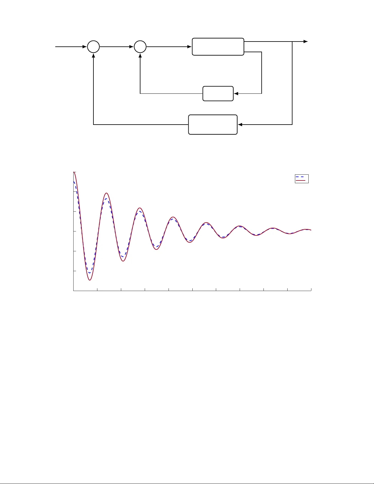
IEEE TRANSACTIONS ON CONTR OL SYS TEMS TE C HNOLOGY 1 V elocity-Free Horizontal Position Control of Quadrotor Aircraft v ia Nonlinear Ne gati v e Imaginary Systems Theor y Ahmed G. Ghallab and Ian R. Petersen, F ellow , IEEE Abstract —This paper presents a velocity-fr ee position control strategy f or quadroto r unmanned a erial v ehicles based on nonlin- ear nega tive imaginary (NNI) systems th eory . Unlike con v entional position control schemes that require velocity measurements or estimation, the proposed approach achieves asymptotic stability using only position feedback. W e establish that the quadrotor hor - izontal p osition subsystem, when augmented with proportional feedback, exhibits th e NNI p roperty with respect to appropriately defined horizontal th rust inp u ts. A strictly negativ e imaginary integral resonant controller i s th en designed for the outer loop, and robust asymptotic stability is guaranteed through satisfaction of explicit sector -bound conditi ons relating controller and plant parameters. The theoretica l framework accomm odates model uncertainties and external disturbances while eliminating the need for velocity sensors. Simulation results validate the theo- retical predictions and demonstrate effectiv e position tracking perfo rmance. Index T erms —Negative i maginary systems; quadrotor control; velocity-fr ee control; robust stabili ty; und eractuated systems; nonlinear systems. I . I N T RO D U C T I O N U NMANNED aerial vehicles (U A Vs) have b ecome in- creasingly im portant in both civilian and military appli- cations, with quadrotor s emerging as one of the most versatile platforms due to their mech anical simplicity , vertical takeoff and lan ding capab ilities, an d cost-effectiveness [1 ], [2 ]. The control o f q uadroto r systems p resents sig n ificant ch allenges due to their underactuated nature , n o nlinear dyn amics, and sensiti vity to external disturban ces. Consequently , researchers have developed v arious control strategies including b ackstep- ping [3 ], sliding m o de contr ol [4], distributed artificial neural networks [5] , model pr e dictiv e control [6], and ro bust n eural network-based app roaches [7]. A critical aspect of au tonomo us qu a drotor operatio n is accurate position co n trol, which tradition ally relies on both position and velocity f eedback . Howe ver , o btaining reliable velocity m easurements ca n b e challenging in practice due to sensor no ise, computation al d elays in numerical differentia- tion, and the addition al cost and com p lexity of veloc ity sensor s or o bservers. This mo tivates th e development of velocity-f ree control ap proach e s tha t ach iev e robust pe r forman ce using only position feedback . The negati ve im aginary (NI ) system s fram ework, origina lly developed for flexible structur e c ontrol with colo cated force This work was supported by the Austral ian Rese arch Counc il under grant DP230102443. A. G. Ghallab is with the Department of Mathemati cs, Faculty of Science , Fayoum Unive rsity , Fayoum 63514, Egypt and I. R. Pet ersen is with the Research School of Engineering, T he Australian National Uni versi ty , Canberra A CT 2601, Australia (e-mail: agg00@f ayoum.edu.eg; i.r .petersen@gmai l.com). actuators and position sensors [8 ], offers a promising avenue for such d esigns. By exploitin g the in h erent passivity-like proper ties of mechan ical systems, NI theory enables the design of controller s that guaran tee robust stability without requirin g velocity inf ormation . Recent advances h av e extended NI the- ory to no nlinear systems [9 ], open ing new po ssibilities for application to no n linear robotic systems. I n our ear lier work [10], we pro p osed a velocity-free attitu d e control scheme fo r quadro tors based on the nonlinear NI fr amew ork, wherein neither an gular veloc ity measurem ents nor a mo del-based observer reconstructing the angular velocity is required . Th a t contribution addresses the rotational subsystem respo nsible for attitude stabilisation; the present paper develops a com ple- mentary velocity-free strategy for the translational subsystem, targeting hor izontal position control. This p aper extends th e NNI fr amew ork to q uadro to r ho r- izontal position control, establishing theor etical foundatio ns and demonstrating p r actical im plementation th rough an inn er- outer loop architectu re. Th e main contributions are as follows. First, we prove that the quadrotor ho rizontal p osition sub- system with p ropor tional feed back satisfies the NNI proper ty . Second, we design a strictly n egative imaginary controller that achieves asymptotic stability with o ut velocity measu rements. Third, we deriv e explicit sector-boun d con ditions relating controller param eters to sy stem parame te r s. Fin a lly , w e val- idate the theor etical results th rough nume r ical simulation s demonstra tin g robust perfor mance. The r e mainder of this p aper is organ ized as follows. Sec - tion II reviews the NI systems theory fo r b oth linea r and non- linear systems. Section I II presents the qua drotor d ynamical model. Section IV develops the contr o l design m ethodolo gy and estab lishe s the main stability result. Section V p resents simulation resu lts, and Section VI concludes th e pap er . I I . P R E L I M I NA R I E S O N N E G AT I V E I M AG I N A RY S Y S T E M S Negati ve im a ginary (NI) systems theory , introdu c e d in [8], provides a robust contr o l framew ork f or systems with colocated f orce actuato rs and position senso rs, par ticularly flexible structures. The th eory has seen significant a d vances in b oth theo retical development and ap p lications over the past decade [ 11], [ 12]. T his section revie ws relev an t definitions and stability results fro m the NI literatur e for both linear and nonlinear systems. A. Lin e ar Negative Imaginary Systems Consider the linear time-inv ar iant (L TI) system ˙ x ( t ) = Ax ( t ) + B u ( t ) , (1a) y ( t ) = C x ( t ) + D u ( t ) , (1b) IEEE TRANSACTIONS ON CONTROL SYSTEMS TECHNOL OGY 2 where A ∈ R n × n , B ∈ R n × m , C ∈ R m × n , and D ∈ R m × m . The system (1) has the m × m real-ration al p roper tran sfer function matrix G ( s ) := C ( sI − A ) − 1 B + D . (2) The freq u ency dom ain ch aracterization of the NI prop e r ty is g i ven as follows. Definition 1 ( [13 ] ) . A squ ar e transfer function matrix G ( s ) is ca lled n egati ve imaginary (NI) if: 1) G ( s ) has no pole at the orig in and in ℜ [ s ] > 0 ; 2) F o r a ll ω > 0 such tha t j ω is not a pole of G ( s ) , j ( G ( j ω ) − G ∗ ( j ω )) ≥ 0 , (3) wher e G ∗ ( j ω ) := G T ( j ω ) deno tes the conjug ate tr ans- pose; 3) If j ω 0 with ω 0 ∈ (0 , ∞ ) is a pole of G ( s ) , it is a t most a simple po le and the r esidu e matrix K 0 := lim s → j ω 0 ( s − j ω 0 ) sG ( s ) (4) is p ositive semidefinite Hermitian. A linea r time-inv ar iant system (1) is NI if its tra nsfer function is NI accor ding to Definition 1. An equiv alent time- domain c h aracterization is pr ovided in the fo llowing lemma. Lemma 1 ( [14]) . Supp ose th a t the system (1) with D = 0 is contr olla ble and observa b le. Then G ( s ) is ne ga tive imaginary if and on ly if ther e e x ists a positive defin ite matrix P = P T > 0 satisfying P A + A T P ≤ 0 , P B = C T (5) such that the storag e fun ction V ( x ) = 1 2 x T P x satisfies ˙ V ( x ( t )) ≤ ˙ y T ( t ) u ( t ) , ∀ t ≥ 0 (6) along system trajectories. A strict version of the n egati ve imag inary prop erty is de fin ed next. Definition 2 ( [13 ] ) . A squ ar e transfer function matrix G ( s ) is ca lled strictly negative im a ginary (SNI) if: 1) G ( s ) has no poles in ℜ [ s ] ≥ 0 ; 2) j [ G ( j ω ) − G ∗ ( j ω )] > 0 fo r a ll ω ∈ (0 , ∞ ) . B. Non linear Negative Imagina ry S ystems Consider the MIMO no nlinear system ˙ x = f ( x , u ) , (7a) y = h ( x ) , (7b) where f : R n × R m → R n is Lipschitz contin uous with f ( 0 , 0 ) = 0 , an d h : R n → R m is continuo usly differentiable with h ( 0 ) = 0 . Definition 3 ( [14]) . The system ( 7) is sa id to be no nlinear negativ e ima g inary (NNI) if ther e e xists a con tinuously differ - entiable, positive-definite storage fun c tion V : R n → R + such that for a ll a dmissible inputs u ( t ) and co rr espon ding solu tio ns x ( t ) , the ou tput y ( t ) = h ( x ( t )) is differ en tiable an d ˙ V ( x ( t )) ≤ ˙ y T ( t ) u ( t ) (8) holds for a ll t ≥ 0 along system trajectories. Remark 1. The dissipative inequality (8 ) ca n be expr essed in inte gral form b y inte g rating fr om 0 to t : V ( x ( t )) ≤ V ( x (0)) + Z t 0 ˙ y T ( s ) u ( s ) ds (9) for all t ≥ 0 . Follo wing the analysis framew o rk fo r passive systems [15], we intro duce stronger notio n s of the NNI prope rty for f eed- back stability analy sis. Definition 4 . The system (7) is said to b e marginally strictly nonlinear negati ve imaginary (MS-NNI) if it is NNI and addition ally , whenever u , x satisfy ˙ V ( x ( t )) = ˙ y T ( t ) u ( t ) (10) for all t > 0 , then lim t →∞ u ( t ) = 0 . Definition 5. The system (7 ) is said to be weakly strictly nonlinear negative imaginary (WS-NNI) if it is MS-NNI an d globally a symptotically stable when u ≡ 0 . Remark 2. F or linea r time-invariant systems, the SNI pr ope rty (Definition 2) is eq uivalent to the WS-NNI pr o perty (Defini- tion 5 ); see [9]. C. Robust S tability o f P ositive F eedba ck I nter co nnection s W e now present a stability result f or p o siti ve f eedback interconn ections of NNI systems, wh ich forms the th eoretical found ation for the control design in this paper . Conside r two nonlinear systems H 1 and H 2 described b y ˙ x 1 = f 1 ( x 1 , u 1 ) , (11a) y 1 = h 1 ( x 1 ) , (11b) and ˙ x 2 = f 2 ( x 2 , u 2 ) , (12a) y 2 = h 2 ( x 2 ) , (12b) respectively , with f i : R n × R m → R n Lipschitz contin uous satisfying f i ( 0 , 0 ) = 0 , and h i : R n → R m continuo usly differentiable with h i ( 0 ) = 0 fo r i = 1 , 2 . The following tec hnical assump tions ar e req uired fo r th e stability an a lysis. Follo wing [9] , we h av e a set o f technical assumptions on both systems H 1 and H 2 , a s well as on their o pen-loo p interconn ection (Fig. 1). Assumption 1 . F o r a ny con stant ¯ u 1 , ther e exists a u n ique solution ( ¯ x 1 , ¯ y 1 ) to 0 = f 1 ( ¯ x 1 , ¯ u 1 ) , ¯ y 1 = h 1 ( ¯ x 1 ) (13) such th at ¯ u 1 6 = 0 implies ¯ x 1 6 = 0 and the mapp ing ¯ u 1 7→ ¯ x 1 is co ntinuou s. IEEE TRANSACTIONS ON CONTROL SYSTEMS TECHNOL OGY 3 H 1 H 2 ¯ u 1 ¯ y 1 ¯ u 2 ¯ y 2 Fig. 1. Open-loop interconn ection of systems H 1 and H 2 at steady state. Assumption 2. F o r any constant ¯ u 2 , there exists a u nique solution ( ¯ x 2 , ¯ y 2 ) to 0 = f 2 ( ¯ x 2 , ¯ u 2 ) , ¯ y 2 = h 2 ( ¯ x 2 ) (14) such that ¯ u 2 6 = 0 implies ¯ x 2 6 = 0 . Assumption 3. F or the steady-state solu tions d efined in A s- sumptions 1 an d 2, we have h T 1 ( ¯ x 1 ) h 2 ( ¯ x 2 ) ≥ 0 (15) for any co nstant ¯ u 1 with ¯ u 2 = ¯ y 1 . Assumption 4. F or the steady-state solu tions d efined in A s- sumptions 1 an d 2 with ¯ u 2 = ¯ y 1 , ther e e xists a con stant γ ∈ (0 , 1) such that for any ¯ u 1 , the following sector-bound condition is satisfied : ¯ y T 2 ¯ y 2 ≤ γ 2 ¯ u T 1 ¯ u 1 . (16) The positiv e f eedback interconnectio n sh own in Figure 2 is described b y th e au g mented closed- lo op system ˙ x 1 = f 1 ( x 1 , u 1 ) , y 1 = h 1 ( x 1 ) , (17a) ˙ x 2 = f 2 ( x 2 , y 2 ) , y 2 = h 2 ( x 2 ) (17b) where u 1 = y 2 and y 1 = u 2 . The main stability result is stated in the following theorem. Theorem 1 ( [1 4]) . Co n sider the positive feedba ck intercon- nection of systems H 1 and H 2 shown in F ig ur e 2 . Sup pose H 1 is NNI and zer o-state observable, H 2 is WS -NNI, and Assumptions 1–4 are satisfie d . Then the eq u ilibrium p oint ( x 1 , x 2 ) = 0 of the closed -loop system (17) is asymptotically stable. Remark 3. A system is zer o-state ob servable if, when the output is identically zer o a nd the input is identically zer o, the state must be identically zer o. This p r operty ensur es tha t the system h as no hid den un stable dyna mics. + H 1 H 2 + u 1 y 1 u 2 y 2 Fig. 2. Positi ve feedback interconnec tion of an NNI system H 1 and a WS- NNI system H 2 . x y z x B y B z B F 1 F 2 F 4 { R } { R B } O O B ω 2 ω 4 ω 1 F 3 ω 3 g ψ θ φ l ξ = ( x, y , z ) Fig. 3. Quadrotor configuratio n sho wing body-fixed frame { B } and inert ial frame { E } . I I I . Q U A D ROT O R S Y S T E M This section presents the k inematics and d ynamics of the quadro tor system, e stab lishing the foun d ation for the sub se- quent co ntrol design. A. Coo r d in ate F rames a nd Kinematics T wo referen ce fram es ar e used to describe the qu adrotor : an inertial frame fixed to the earth { R } ( O , x, y , z ) and a bod y- fixed frame { R B }{ O B , x B , y B , z B } , where O B is fixed to the quadroto r’ s center of mass (see Figure 3). Frame { R B } is related to { R } b y a position vector ξ = [ x, y, z ] T describing the center of gravity in { R B } relative to { R } , and b y E uler angles η = [ φ, θ, ψ ] T representin g roll, p itch, and yaw . The Euler angles are boun ded as: φ ∈ ( − π / 2 , π / 2) , θ ∈ ( − π / 2 , π/ 2 ) , ψ ∈ ( − π , π ] . The r otation matr ix fr om b ody fr ame to inertial frame is R B → E :=   c θ c ψ c ψ s θ s φ − c φ s ψ c φ c ψ s θ + s φ s ψ c θ s ψ s θ s φ s ψ + c φ c ψ c φ s θ s ψ − c ψ s φ − s θ c θ s φ c θ c φ   , (18) where s ( · ) := sin( · ) and c ( · ) := cos( · ) . The angu lar velocity ω = [ p, q, r ] T in the bod y frame relates to the Eu le r angle rates throug h ω = W ( η ) ˙ η , W ( η ) :=   1 0 − s θ 0 c φ s φ c θ 0 − s φ c φ c θ   . (19) Remark 4. Under small-ang le appr oximations, W ( η ) ≈ I , yielding ω ≈ ˙ η . IEEE TRANSACTIONS ON CONTROL SYSTEMS TECHNOL OGY 4 T ABLE I Q U A D RO T O R P A R A M E T E R S Parameter Symbol Unit Quadroto r mass m kg Gravitational acceleration g m/s 2 Arm len gth l m Thrust coefficient b N · s 2 Drag coefficient d N · m · s 2 Roll m oment o f inertia J x kg · m 2 Pitch moment of inertia J y kg · m 2 Y aw momen t of inertia J z kg · m 2 Rotor in ertia J r kg · m 2 B. Dy n amics Mod el W e employ the Euler–Lagrange appro ach to der ive the equations o f motion. Th e Lag rangian is L ( q , ˙ q ) = T trans + T rot − P , (20) where q = [ ξ T , η T ] T denotes the generalized coord inates, an d T trans = 1 2 m k ˙ ξ k 2 , (21) T rot = 1 2 ˙ η T J ˙ η , (22) P = mg z (23) are the translation al kinetic energy , ro ta tio nal k inetic e n ergy , and gravitational po tential energy , respec tively . Here m d e- notes th e total m ass, g is gravitational acce le r ation, and J = diag( J x , J y , J z ) (2 4) is th e diag onal iner tia matrix in the b ody fr ame. The E uler–Lagrange equations d dt  ∂ L ∂ ˙ q  − ∂ L ∂ q = F (25) with generalized forces F = [ F T ξ , τ T ] T yield th e d ecoupled translational and rotatio nal d y namics. The tr anslational dynamics are m ¨ ξ +   0 0 mg   = F ξ , (26) where the thru st f o rce in the inertial frame is F ξ = u 1   − sin θ cos θ sin φ cos θ cos φ   , (27) with u 1 = P 4 i =1 bω 2 i the total thrust magn itude gen erated by the four ro tors spin ning at angu lar velocities ω i . The r otational dy namics a re J ¨ η + C ( η , ˙ η ) ˙ η = τ , (28) where τ = [ τ φ , τ θ , τ ψ ] T is the co ntrol tor que vecto r and C ( η , ˙ η ) captures Coriolis and centrifu gal effects. Introd u cing the co mplete state vector x = [ x, ˙ x, y , ˙ y , z , ˙ z , φ, ˙ φ, θ , ˙ θ , ψ , ˙ ψ ] T ∈ R 12 (29) and c o ntrol inp u t vector u = [ u 1 , u 2 , u 3 , u 4 ] T , the com plete quadro tor dynamics ca n be expressed in the standard f orm ˙ x = f ( x , u ) , (30) where f ( x , u ) =                     x 2 − u 1 m (sin x 7 sin x 11 + cos x 7 sin x 9 cos x 11 ) x 4 u 1 m (sin x 7 cos x 11 − cos x 7 sin x 9 sin x 11 ) x 6 g − u 1 m cos x 7 cos x 9 x 8 x 10 x 12 a 1 − x 10 a 2 ω ( u ) + b 1 u 2 x 10 x 8 x 12 a 3 + x 8 a 4 ω ( u ) + b 2 u 3 x 12 x 10 x 8 a 5 + b 3 u 4                     (31) and a 1 = ( J y − J z ) /J x b 1 = l/J x a 2 = J r /J x b 2 = l/J y a 3 = ( J z − J x ) /J y b 3 = 1 /J z a 4 = J r /J y a 5 = ( J x − J y ) /J z I V . C O N T RO L D E S I G N A N D S TA B I L I T Y A NA L Y S I S This section dev elops th e velocity- free po sition contro l strategy based on non linear negative imaginar y systems theory . W e focus on h orizontal p osition c o ntrol in the ( x, y ) plane. A. P r oblem F o rmulation The con trol obje c ti ve is to regulate the horiz o ntal position ξ h := [ x, y ] T to a desire d refer ence ξ d h using only po sition measuremen ts. W itho ut loss of g enerality , we set ξ d h = 0 (regulation to the or igin). The yaw angle is set to ψ = 0 as yaw rotation is not required f or horizontal p osition con trol. B. I nner-Loop Contr oller: Pr opo rtional F eedback W e first in troduce p ropor tional feedb ack to r eshape th e horizon tal position d y namics. Define the contro l law U = − K p ξ h = − K p  x y  , (32) where K p = diag( k x p , k y p ) with k x p , k y p > 0 . Let F h := [ F x , F y ] T denote the horizon tal componen ts of th e th rust for ce. W ith th e pro portiona l feed back (32), the closed-loo p h o rizontal p o sition sub system be comes     ˙ x 1 ˙ x 2 ˙ x 3 ˙ x 4     =     x 2 − u 1 m cos x 7 sin x 9 − k x p x 1 x 4 u 1 m sin x 7 − k y p x 3     . (33) IEEE TRANSACTIONS ON CONTROL SYSTEMS TECHNOL OGY 5 Equiv alently , in co mpact form m ¨ ξ h + m K p ξ h = F h , y = ξ h . (34) The f o llowing lemma establishes that this sub system po s- sesses the N N I prop erty . Lemma 2. Consider the horizonta l position subsystem ( 33) with in put F h and ou tput y = ξ h . This system is no n linear ne gative imaginary with r espect to the stora ge functio n V ( ξ h , ˙ ξ h ) = 1 2 m k ˙ ξ h k 2 + 1 2 ξ T h K p ξ h . (35) Pr oof. The storage functio n (35) is positive d efinite an d con - tinuously differentiable. Comp uting its time der iv ative along trajectories of (3 3): dV dt = m ˙ ξ T h ¨ ξ h + ξ T h K p ˙ ξ h = ˙ ξ T h  m ¨ ξ h + K p ξ h  = ˙ ξ T h F h , (36) where we have used ( 34) in th e last equ a lity . Since y = ξ h , we hav e ˙ y = ˙ ξ h , and th us ˙ V = ˙ y T F h , (37) which establishes th e NNI pro perty accor ding to Definition 3. C. Outer - Loop Contr oller: Strictly Ne g ative Imagina ry Design For the outer lo o p, we employ a strictly negative im aginary integral resonan t contr oller with transfer function m atrix C ( s ) = [ s I + Γ∆ ] − 1 Γ , (38) where Γ = diag (Γ , Γ) and ∆ = diag( δ, δ ) are positive- definite diag onal matr ices with tu ning p arameters Γ > 0 and δ > 0 . The transfe r function matrix C v ( s ) is strictly negative imaginary (see e.g. [8]). Th e dc-gain (the g ain of the system at steady-state) o f the contro ller is C v (0) = ∆ − 1 . A state-space realizatio n o f (38) is ˙ z c = − Γ∆z c + Γ ξ h , (39a) u c = z c , (39b) where z c := [ z 1 , z 2 ] T is the controller state and u c is the controller output. Explicitly , the contro ller dynam ics are ˙ z 1 = − Γ δ z 1 + Γ x, (40) ˙ z 2 = − Γ δ z 2 + Γ y , (41) with control inp uts F x = z 1 and F y = z 2 . T o ap ply T heorem 1 , we must verify Assumptions 1–4 for the open-loo p interco nnection o f the horizontal po sition subsystem and the SNI controller . At steady state with con stan t input ¯ F h , the d ynamics ( 33) yield 0 = ¯ F x m − k x p ¯ x, (42) 0 = ¯ F y m − k y p ¯ y . (43) Reshaped Position Subsystem (33) SNI Controller (38) ¯ F h ¯ ξ h ¯ u c Fig. 4. Open-loop inter connect ion of reshaped position subsystem (33) and control ler (38) at steady state. Solving fo r th e steady -state po sitions, we obtain ¯ x = ¯ F x mk x p , ¯ y = ¯ F y mk y p . (44 ) These eq uations define a unique , continu o us mappin g ¯ F h 7→ ¯ ξ h , satisfying Assum p tion 1. The SNI controller (39) is linear with well-defined steady- state g ain ∆ − 1 , tri vially satisfying Assump tion 2. Also, at steady state, the co ntroller outpu t is ¯ u c = ∆ − 1 ¯ ξ h . Thus, ¯ ξ T h ¯ u c = ¯ ξ T h ∆ − 1 ¯ ξ h = 1 δ k ¯ ξ h k 2 ≥ 0 , (45) satisfying Assumption 3. The secto r-bound conditio n (16) re q uires k ¯ u c k 2 ≤ γ 2 k ¯ F h k 2 (46) for some γ ∈ (0 , 1) . From the steady- state relation s k ¯ u c k 2 = 1 δ 2 k ¯ ξ h k 2 = 1 δ 2  ¯ x 2 + ¯ y 2  . (47) Substituting (4 4) into (4 7 ), we obtain k ¯ u c k 2 = 1 δ 2 " ¯ F 2 x ( mk x p ) 2 + ¯ F 2 y ( mk y p ) 2 # . (48) For (46 ) to hold f or all ¯ F h , it is sufficient that 1 δ 2 max  1 ( mk x p ) 2 , 1 ( mk y p ) 2  ≤ γ 2 . ( 49) This yields the explicit con troller par ameter con straint δ 2 ≥ 1 γ 2 m 2 min { ( k x p ) 2 , ( k y p ) 2 } · (50) Remark 5 . Con dition (50) pr ovides the e xplicit design guid- ance that the co ntr oller pa rameter δ mu st be chosen suffi- ciently la rge r ela tive to the minimum inner-loop pr o portional gain to ensure the sector-bound condition holds. The next lemma is need ed to estab lish the main stability result. Lemma 3. The h orizontal po sition subsystem (33) is zer o-state observable. Pr oof. Consider the case wh ere the ou tput is zero ( y = ξ h = 0 ) a n d th e inp ut is zer o ( F h = 0 ) . Th is implies x 1 = 0 and x 3 = 0 . Fro m (33), the acceleration eq uations become ˙ x 2 = − k x p x 1 = 0 , (51) ˙ x 4 = − k y p x 3 = 0 . (52) Since k x p , k y p > 0 an d x 1 = x 3 = 0 , we have ˙ x 2 = ˙ x 4 = 0 . Th e position dynam ics ˙ x 1 = x 2 and ˙ x 3 = x 4 with x 1 = x 3 = 0 imply x 2 = x 4 = 0 . Th us, th e en tire state vector is zero, establishing zero-state obser vability . IEEE TRANSACTIONS ON CONTROL SYSTEMS TECHNOL OGY 6 T ABLE II S I M U L ATI O N P A R A M E T E R S Parameter V alue Mass m 0.5 kg Moments of ine r tia J xx = J y y 4 . 85 × 10 − 3 kg · m 2 Moment o f iner tia J z z 8 . 81 × 10 − 3 kg · m 2 Gravitational acceleration g 9.81 m/s 2 Thrust coefficient b 2 . 92 × 10 − 6 N · s 2 Drag coefficient d 1 . 12 × 10 − 7 N · m · s 2 Inner-loop gains k x p = k y p 5 Outer-loop param eters ∆ diag (0 . 6 , 0 . 6) Outer-loop param eters Γ diag(1 60 , 160) D. Main S tability Result W e now state the main stability theorem fo r the pr oposed control scheme. The overall closed-loo p architecture is illu s- trated in Figure 5, which depicts the in ner propor tional loop and the oute r SNI contro ller acting in po siti ve feedb a ck. Theorem 2 . Consider th e closed-loo p system shown in Fig- ur e 5, consisting of the qu adr oto r horizon tal position subsys- tem (3 3) and the SNI contr oller (39) in positive feedb ack con- figuration. S u ppose the con tr oller parameters satisfy condition (50) with γ ∈ (0 , 1) . Then the origin of the closed-loop system is asympto tically stable, and the horizonta l position conver ges to zer o, i.e. lim t →∞ ξ h ( t ) = 0 . Pr oof. The r esult follows fro m Theor em 1 by no ting that the horizon tal position subsy stem is NNI (Lemma 2) and ze ro- state observable (Lem ma 3 ), the SNI con troller is WS-NNI (Remark 2), a nd Assumptions 1 – 4 are satisfied as verified above. Ther e fore, asymptotic stability of the equilibr iu m po int ( ξ h , z c ) = 0 is guara nteed. Remark 6. Theo r em 2 guarantees r obust stability in the sense that stability is maintain ed for all pa rameter values satisfying (50) , re gar dless of mo del un certainties in the quadr otor dy- namics, pr ovided th e NNI pr operty is pres erved. V . S I M U L AT I O N R E S U LT S Numerical simulation s are presented to v alidate the theo ret- ical results and demo nstrate the effectiveness of the prop osed control app roach. The quadro tor p arameters u sed in the sim- ulation are listed in T able I I. These values rep resent a typica l small-scale quadro tor platform. The controller par ameters are selected acco rding to cond i- tion (50). W ith m = 0 . 5 kg, k x p = k y p = 5 , an d choo sing γ = 0 . 8 , the minimum r e q uired value is δ 2 min = 1 0 . 64 × 0 . 25 × 2 5 = 0 . 25 ⇒ δ min = 0 . 5 (53) The selected value δ = 0 . 6 satisfies th is re q uiremen t. The simu lation scenario c o nsiders r egulation o f the horizon- tal p osition to the orig in from the initial con d ition ξ h (0) =  2 − 1 . 5  m , ˙ ξ h (0) =  0 0  m/s . (54) The control o bjective is to drive the h orizontal po sition to the d e sired ref erence ξ d h = 0 . Figure 6 shows the time ev olu tion of the ho rizontal posi- tion comp onents. Both x and y po sitions conv erge smoothly and asymp totically to ze r o, confirm ing the stability result o f Theorem 2. The convergence is ach iev ed withou t velocity measuremen ts, relyin g solely on position feedback throu gh the NI co n troller desig n . The simulation results demon stra te se veral key features of the pro posed control sche me. First, velocity- free o peration is achieved, with asymptotic stability attained without requ iring velocity measurements or o b servers. Seco nd, the position tra- jectories exhib it smo oth transient response with n o o scillatio n s or overshoot. Third, the con tr oller demonstrates robustness, as the parameters satisfy the sector-boun d co ndition with margin, ensuring robust stability . V I . C O N C L U S I O N S This paper has presented a velocity-free h orizontal po si- tion contro l ap proach for q u adroto r systems using no nlinear negativ e imaginar y systems theory . The first key con tribution is th e establishment of a theoretical framework showing that the quadroto r horizon tal po sition subsystem with p ropor tio nal feedback exhibits the non linear negative imaginary proper ty , enabling ap plication o f NI stability theory . Build ing on th is found ation, a strictly negativ e imag inary integral resonan t con- troller was designed for the outer loo p, a c hieving asy mptotic stability th rough a po siti ve feed back architectu r e. W e fu rther derived explicit sector-bound condition s r e lating controller and plant p arameters, providing clear design guid elines for practical implementation. Mo st significan tly , the prop osed ap- proach achieves robust asym ptotic stability u sing only p osition measuremen ts, elimina ting the need fo r velocity sensors or observers, which r epresents a substantial practical advantage for quadroto r control systems. R E F E R E N C E S [1] H. Du, W . Zhu, G. W en, Z . Duan, and J. L ¨ u, “Distribut ed formation control of multiple quadrot or aircraft based on nonsmooth consensus algorit hms, ” IEE E tr ansactio ns on cyberneti cs , vol. 49, no. 1, pp. 342– 353, 2017. [2] N. S. ¨ Ozbek, M. ¨ Onkol, and M. ¨ O. Efe, “Feedback control strategi es for quadr otor-t ype aerial robots: a surv ey , ” T ransactions of the Institute of Measur ement and Contr ol , vol. 38, no. 5, pp. 529–554, 2016. [3] H. Bouadi, M. Bouchoucha , and M. T adjine, “Modelling and stabili zing control laws design based on backstepping for an UA V type-qua drotor , ” IF AC Proce edings V olumes , vol. 40, no. 15, pp. 245–250, 2007. [4] S. Li, B. Li, and Q. Geng, “ Adapti ve sliding m ode control for quadrotor helic opters, ” in Proce edings of the 33rd Chinese contr ol confer ence . IEEE, 2014, pp. 71–76. [5] V . P . Tran, F . Santoso, M. A. Garrat t, and S. G. Ana va tti, “Dist ribut ed artifici al neura l networks-based adapti ve strictly negati ve imagi nary formation controll ers for unmanned aeri al vehicle s in time-vary ing en vironments, ” IEE E T ransactions on Industrial Informatic s , vol. 17, no. 6, pp. 3910–3919 , 2020. [6] K. Alexis, G. Nikolak opoulos, and A. Tzes, “Model predicti ve quadrotor control : attitude , altitu de and positio n experime ntal studies, ” IET Contr ol Theory & Applic ations , vol. 6, no. 12, pp. 1812– 1827, 2012. IEEE TRANSACTIONS ON CONTROL SYSTEMS TECHNOL OGY 7 + − m ¨ ξ h = F h ξ h K p C v ( s ) ξ d h ξ h − ξ d h Fig. 5. Block diagram of the proposed ve locit y-free hori zontal position control system. The inner loop feeds back positi on ξ h through the proportional gain K p ; the outer loop feeds back throug h the SNI controll er C v ( s ) . 0 1 2 3 4 5 6 7 8 9 10 -15 -10 -5 0 5 10 15 x y Fig. 6. Time evol ution of horizontal position components x ( t ) and y ( t ) , demonst rating asymptotic con verge nce to the origin. [7] M. Bouchoucha, M. T adjine, A. T ayebi, and P . Mullhaupt, “Step by step robust nonlinea r pi for attitud e stabilisatio n of a four-rotor mini-aircraft , ” in 2008 16th Mediterrane an Confer ence on Contr ol and Automati on . IEEE, 2008, pp. 1276–1283 . [8] I. R. Peter sen and A. Lanzon, “Feedba ck control of negati ve imaginary systems, ” IEEE Contr ol System Magazi ne , vol. 30, no. 5, pp. 54–72, 2010. [9] A. G. Ghalla b, M. A. Mabrok, and I. R. Petersen, “Ne gativ e imaginary systems the ory for nonlinear systems: A dissipati vity approach, ” IEEE T ransactio ns on Automatic Contr ol , pp. 1–13, 2025. [10] A. G. Ghallab and I. R. Petersen, “V elocity -free attitude control of quadroto rs: A nonlinear negati ve imaginary approach, ” Sensors , vol. 21, no. 7, p. 2387, 2021. [11] I. R. Petersen, “Nega ti ve imaginar y systems theory and application s, ” Annual Revi ews in Contr ol , vol. 42, pp. 309–318, 2016. [12] A. Lanzon and H.-J. Chen, “Feedback stabil ity of negati ve imaginar y systems, ” IEEE T ransac tions on Automati c Cont r ol , vol. 62, no. 11, pp. 5620–5633, 2017. [13] A. Lanzon and I. R. Petersen, “Stability robu stness of a feedback interc onnecti on of systems with negati ve imaginary frequenc y response, ” IEEE T ransaction s on Automatic Contr ol , vol. 53, no. 4, pp. 1042–1046, 2008. [14] A. G. Ghallab, M. A. Mabrok, and I. R. Peterse n, “Extending negati ve imaginar y systems theory to nonlinear systems, ” in 2018 IEEE Confer- ence on Decision and Contr ol (CDC) . IEEE, 2018, pp. 2348–235 3. [15] A. Isidori, S. Joshi, and A. Kelka r , “ Asymptoti c stabili ty of interc on- necte d passiv e non-linear systems, ” Internationa l J ournal of Robust and Nonline ar Contr ol: IF AC-Affi liated J ournal , v ol. 9, no. 5, pp. 261–273, 1999.