Control Forward-Backward Consistency: Quantifying the Accuracy of Koopman Control Family Models

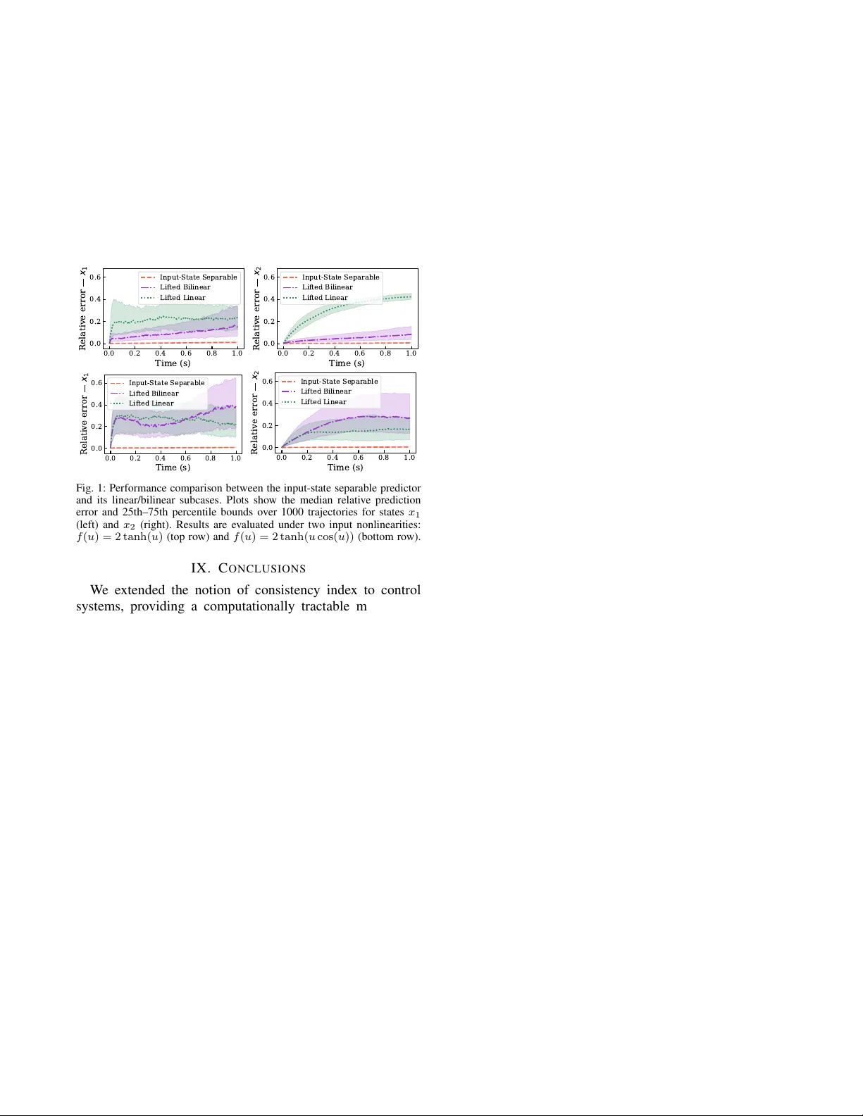
Control Forw ard-Backward Consistenc y: Quantifying the Accuracy of K oopman Control F amily Models Masih Haseli Jorge Cort ´ es Joel W . Burdick Abstract — This paper extends the forward-backward consis- tency index, originally introduced in Koopman modeling of sys- tems without input, to the setting of contr ol systems, providing a closed-f orm computable measure of accuracy for data-driven models associated with the Koopman Control Family (KCF). Building on a forward-backward r egression perspecti ve, we introduce the contr ol forward-backward consistency matrix and demonstrate that it possesses several fav orable properties. Our main result establishes that the relative root-mean-square error of KCF function pr edictors is strictly bounded by the square root of the control consistency index, defined as the maximum eigen value of the consistency matrix. This pro vides a sharp, closed-form computable error bound for finite-dimensional KCF models. W e further specialize this bound to the widely used lifted linear and bilinear models. W e also discuss how the control consistency index can be incorporated into optimization- based modeling and illustrate the methodology via simulations. I . I N T RO D U C T I O N K oopman-based surrogate modeling has become popular in controls and robotics, with many applications relying on finite-dimensional K oopman-inspired models. Since the quality of the resulting closed-loop behavior directly depends on the accuracy of the underlying model, measuring this accuracy is of utmost importance. A proper accuracy measure is essential not only for v erification but also for reliable construction of data-driv en models (e.g., as a loss function). This paper develops such a measure for control systems. Literatur e Review: The K oopman operator represents a dynamical system without input via a linear operator on a function space [1]. The operator’ s action on a function encodes its evolution under composition with the system dynamics. This enables one to study nonlinear dynamical systems using the regular structure of linear operators on vector spaces. Although the original K oopman operator defi- nition does not account for system inputs, there are numerous successful use cases of Koopman-based/inspired methods in controls, e.g. optimal [2], robust [3], and safety-critical [4]. Many prior works do not rely on a formal extension of the K oopman operator to control systems; instead, they rely on “lifted” models inspired by the finite-dimensional form of Koopman operators for systems without input [5, Section 1.4]. Lifted linear forms [6] are widely used for their compatibility with linear control methods. Ho wev er , M. Haseli and J. W . Burdick are with the Division of Engineering and Applied Science, California Institute of T echnology , Pasadena, CA 91125, USA, { mhaseli, jburdick } @caltech.edu . J. Cort ´ es is with the Department of Mechanical and Aerospace Engineering, University of California, San Diego, CA 92093, USA, cortes@ucsd.edu . The work of M. Haseli and J. Burdick was supported by the T echnology Innov ation Institute of Abu Dhabi and D ARP A under the LINC program. The w ork of J. Cort ´ es w as supported by ONR A ward N00014-23-1-235. such forms do not capture input nonlinearities or the input- state coupling. The work [7] provides necessary and suf fi- cient conditions on the system dynamics to admit a finite- dimensional lifted linear model. Moreover , [8] studies and tackles the limitations of lifted linear models via oblique pro- jections. Bilinear forms are another widely used K oopman- based surrogate model, often associated with control-af fine systems. The work [9] studies the properties of K oopman generators associated with control-affine systems and surro- gate bilinear models while [10] studies a similar problem through the lens of geometric control. W e refer the reader to [11] for a revie w of Koopman-based control and error bounds, especially for lifted linear and bilinear models. General non-affine control systems can be handled in a K oopman framework by setting the control input to be a con- stant, whereupon the system admits a traditional Koopman operator . Thus control inputs can be handled by switching between the K oopman operators for finitely many constant- input systems. This idea has been used numerous times, for purposes such as PDE control [12], control of monotone systems [2], and sampling-based control design [13]. While the bulk of the literature studied K oopman-based surrogate models, rigorous extensions of K oopman theory to general (not necessarily control affine) nonlinear control sys- tems have receiv ed less attention. [14] builds a rigorous ex- tension of K oopman operator theory to general discrete-time control systems by considering all possible behaviors arising from infinite-input sequences. Alternativ ely , [15] introduces the K oopman Contr ol F amily (KCF) formalism, using all possible K oopman-operators associated with all constant- input systems. Later , it was shown in [16] that under certain conditions on the function spaces, the infinite-input sequence paradigm [14] is in fact equiv alent to KCF [15], although the theoretical structures look very different. Alternatively , [17] provides a different extension of the Koopman operator to control systems based on product spaces. This paper studies the accuracy of finite-dimensional forms associated with the KCF framew ork in data-driv en settings. W e extend the forward-backward consistency index from [18], originally defined for systems without input, to control systems. The notion of forward and backward dynamics has been used numerous times in the literature, including to deal with noise [19], [20], forecasting [21], and identifying approximately K oopman-in variant subspaces [22] among many other applications. Statement of Contrib utions: W e extend the consistency index used for Koopman-based modeling of systems without input [18] to control systems, and thereby dev elop an ac- curacy measure for input-state separable models associated with the Koopman Control Family (KCF) for data-dri ven settings. Adopting a forward-backward regression perspec- tiv e, we introduce the contr ol forwar d-backwar d consistency matrix (CFBCM). W e show that this matrix has sev eral desirable properties: (i) it is similar to a positive-semidefinite matrix; (ii) its eigen values are real and belong to the interval [0 , 1] , and (iii) these eigen values do not depend on the choice of bases. This inv ariance of the spectrum under the choice of basis is quite meaningful since function predictors in the KCF are also independent of the choice of basis. Our main result establishes that the relativ e root-mean-square error of KCF function predictors admits a sharp upper bound deter- mined by the square root of the largest CFBCM eigen value (which we define as the contr ol consistency index ), leading to a closed-form error bound. W e also show how this bound can be specialized to the widely used lifted linear and bilinear subclasses of input-state separable models. Finally , we show how our results can be used in optimization-based modeling and provide guidelines for improving training ef ficiency 1 . I I . A P R I M E R O N K O O P M A N C O N T R O L F A M I L Y Here, we provide a few necessary definitions and results from the K oopman Control Family (KCF) frame work follow- ing [15] that we use throughout the paper . Consider the (not necessarily control-affine) discrete time dynamical system x + = T ( x, u ) , x ∈ X ⊆ R n , u ∈ U ⊆ R m . (1) By setting input u to be a constant, one can use (1) to create a family of systems without input { x + = T u ∗ ( x ) := T ( x, u ≡ u ∗ ) } u ∗ ∈U . (2) Giv en that the family of systems (2) do not have inputs, the traditional definition of the Koopman operator can be applied to the family , leading to the definition of the KCF . Definition II.1: (K oopman Contr ol F amily [15, Defini- tion 4.1]): Consider F , a vector space of complex-v alued functions with domain X that is closed under composition with elements of the family (2), i.e., f ◦ T u ∗ ∈ F , for all f : X → C in F and all u ∗ ∈ U . The K oopman Control Family (KCF) is defined as {K u ∗ : F → F } u ∗ ∈U , where K u ∗ f = f ◦ T u ∗ , ∀ f ∈ F , ∀ u ∗ ∈ U . □ 1 W e denote the sets of natural, non-negati ve integer , real, and complex numbers by N , N 0 , R , and C . For matrix A ∈ C m × n , we use A T , A ∗ , ∥ A ∥ F , A † , Row( A ) , and cond ( A ) to denote its transpose, conjugate transpose, Frobenius norm, pseudoinv erse, row space (the vector space spanned by rows), and condition number . If A is square, T r( A ) , A − 1 , and spec( A ) denote its trace, inverse, and spectrum. If sp ec( A ) ⊂ R , λ max ( A ) denotes its maximum eigenv alue. If A is positive semidefinite, A 1 2 denotes its square root. For matrices A and B with the same number of rows, [ A, B ] denotes the side-by-side concatenation of A and B . 0 m × n and I m represent the m × n zero matrix and m × m identity matrix respectively (indices are omitted when clear). For v ∈ C n , ∥ v ∥ denotes its 2 -norm. For vector space V , dim( V ) denotes its dimension. For function Ψ : X → C n , span(Ψ) denotes the vector space spanned by its elements. Also, for set S ⊆ V , span( S ) ⊆ V denotes the vector space spanned by S . Giv en f : A → B and g : B → C , g ◦ f : A → C denotes their composition. For sets B ⊆ A where A is equipped with a metric d , we say y is the best approximation of x ∈ A on B denoted by x best ≈ B y if y ∈ arg min z ∈ B d ( x, z ) . The KCF can fully encode the trajectories of (1) in the ev olution of functions in F : gi ven initial condition x 0 and an input sequence { u t } t ∈ N 0 , then f ( x t ) =  K u 0 · · · K u t − 1 f  ( x 0 ) , ∀ f ∈ F , ∀ t ∈ N 0 . (3) A. P arameterizing KCF via Augmented K oopman Operator Since the KCF may contain uncountably many operators, utilizing it in an efficient manner requires an ef fectiv e pa- rameterization. T o this end, we first parameterize the family of constant-input systems (2) via the following system that acts on the augmented state space X × U ( x, u ) + = T aug ( x, u ) := ( T ( x, u ) , u ) . (4) Note that the augmented system T aug in (4) does not hav e an input, and u is a part of the state. System (4) completely cap- tures the family of constant input systems [15, Lemma 5.1]. Giv en that (4) is a system without input, we can define a K oopman operator K aug : F aug → F aug as K aug g = g ◦ T aug , ∀ g ∈ F aug , (5) where F aug is an appropriate function space closed under composition with T aug . Interestingly , K aug can parameterize the members of the KCF giv en mild conditions on function spaces F aug and F : see [15, Definition 5.4]. The most important condition, which we use frequently , is f ◦ T ∈ F aug for all f ∈ F . W e refer the reader to the discussion after [15, Definition 5.4] for examples for choices of F and F aug . B. F inite-Dimensional F orms of KCF For computational reasons, one naturally seeks finite- dimensional approximations to the KCF . Finite-dimensional models arise from the principle of subspace inv ariance: if a model’ s input and output are to lie in a given finite- dimensional subspace, that subspace must be inv ariant under the action of the model . For dynamical systems without input, finite-dimensional K oopman-based models follow the same principle: their form is dictated by subspaces that are in variant under the K oopman operator , leading to the well- known lifted linear model. The same form is used for non- in variant subspaces through appr oximations 2 . T o obtain a finite-dimensional form for the KCF using the inv ariance principle, let H : X → C n H be such that its elements form a basis for a KCF’ s common in variant subspace, denoted by H ⊆ F . The finite-dimensional form of the KCF , termed the “input-state separable” model, is H ◦ T = A H, (6) where A : U → C n H × n H is a matrix-v alued function. Evaluating (6) on a pair ( x, u ) ∈ X × U gives H ( x + ) = H ◦ T ( x ) = A ( u ) H ( x ) , leading to the following point-wise dynamic predictor 3 z + = A ( u ) z , z ∈ C n H , u ∈ U . (7) 2 These approximations often in volve composing projection operators with the K oopman operator to generate an approximate operator that renders the underlying subspace inv ariant [5, Section 1.4]. 3 Since Koopman operators act on functions; Eq. (6) is a fundamental no- tion, while its point-wise ev aluation (7) is simply a useful byproduct. Later, for the case of non-in variant subspaces, we study function approximations. Giv en trajectory { x k } k ∈ N 0 generated from the initial con- dition x 0 and input sequence { u k } k ∈ N 0 , if we initialize (7) with z 0 = H ( x 0 ) , we have z k = H ( x k ) for all k ∈ N 0 . Remark II.2: (Generality of Input-State Separable Mod- els): The input-state separable form (7) is the general finite- dimensional form of the KCF following [15, Theorem 4.3]. The lifted linear , bilinear , and switched linear models that are widely used in the Koopman literature are special cases of input-state separable models [15, Lemmas 4.5–4.6]. □ Eq. (7) is linear in the “lifted state” z , but is generally nonlinear in u . This nonlinearity in the input is unav oidable whenev er system (1) is nonlinear in the input. Finite-dimensional in variant subspaces containing the de- sired functions may not be easy to identify , or even exist. In such cases, we use an approximate form of (6) H ◦ T ≈ A H . (8) T o approximate the action of functions on trajectories, one still uses (7) with A in (8); howe ver , the action of H on trajectories of (1) deviates from the trajectories of (7), and this deviation depends on the quality of approximation in (8). It is important to note that (8) provides a predictor not only for the ev olution of elements of H , but also for all elements of H = span( H ) . Indeed, giv en h ∈ H with representation h = v ∗ h H for some v h ∈ C n H , the approximation of h ◦ T induced by (8), denoted by P h ◦T , is given by h ◦ T ≈ P h ◦T := v ∗ h A H . (9) The approximations in (8)–(9) are obtained via projections, defined according to the structure of F and F aug . Next, we describe ho w K aug can be used to construct optimal predictors when F aug is endo wed with an inner product ⟨· , ·⟩ inducing a norm ∥ · ∥ . T o this end, we rely on the following subspaces. Definition II.3: (Non-de generate Normal Subspaces in F aug and Their Bases [15, Definition 7.1]): Let the elements of Ψ : X × U → C n Ψ be linearly independent. W e say Ψ is in (non-degenerate) normal separable form (or normal form for short) if it can be decomposed as Ψ =  I U G  H (10) where H : X → C n H , G : U → C ( n Ψ − n H ) × n H and function I U : U → C n H × n H returns the identity matrix, I U ( u ) = I for all u ∈ U . W e say that S ⊂ K aug is a normal subspace if its basis can be written in normal form 4 . □ The next result connects the finite-dimensional approxi- mations of K aug on S = span(Ψ) ⊆ F aug to the input-state separable forms on H = span( H ) ⊆ F . Theor em II.4: (Optimal Appr oximation of Input-State Separable F orms fr om K aug [15, Theor em 8.7]): Gi ven Ψ and H in (10), let S = span(Ψ) ⊆ F aug , H = span( H ) , and let P S : F aug → F aug be the orthogonal projection operator on S . Let A ∈ C n Ψ × n Ψ be a matrix such that P S K aug Ψ = A Ψ 4 In (10), I U and G are matrix-valued functions with domain U and H is a vector-v alued function with domain X . The matrix products are defined in an element-wise sense similar to numerical matrix and vector products. (this matrix exists since S is always in variant under P S K aug ). Decompose A in blocks as follows A =  A 11 A 12 A 21 A 22  , (11) where A 11 ∈ C n H × n H . Then, (a) for all h = v ∗ h H ∈ H , with v h ∈ C n H , define P h ◦T := v ∗ h ( A 11 I U + A 12 G ) H ∈ S . (12) Then, P h ◦T is the best approximation (orthogonal pro- jection) of h ◦ T on S , i.e., h ◦ T best ≈ S P h ◦T . (b) H ◦ T best ≈ S ( A 11 I U + A 12 G ) H , where best ≈ S is defined element-wise. □ Theorem II.4 pro vides a practical way to find best ap- proximations of input-state separable models for KCF via approximations of the action of a single linear operator . The predictors P h ◦T in Theorem II.4 only depend on the choice of normal space S and not on the choice of normal basis Ψ , as detailed below . Lemma II.5: (In variance of Function Pr edictors in Theo- r em II.4 under choice of Normal Basis): Let P h ◦T and ¯ P h ◦T be predictors of h ◦ T with respect to normal bases Ψ and ¯ Ψ with S = span(Ψ) = span( ¯ Ψ) . Then, P h ◦T = ¯ P h ◦T . □ The proof follows from the fact that P h ◦T and ¯ P h ◦T are or - thogonal projections of h ◦ T on S ; hence, the result trivially follows from the uniqueness of orthogonal projections 5 . I I I . D A TA - D R I V E N S E T U P A N D P R O B L E M S T A T E M E N T K oopman operator-based methods are widely used in data- driv en settings since they utilize the computationally and theoretically attractive regular structure of linear maps acting on vector spaces. W ith this motiv ation, we study the accuracy of optimal approximate models in Theorem II.4 in a data- driv en setting. T o achiev e this goal, we first pro vide a proper data-driv en setup and then introduce our main problem. A. Data-Driven Setup T o apply Theorem II.4, we need to provide a notion of data from system (1), explain how one can ev aluate the normal basis (10) on the data, and provide a useful notion of inner- product on F aug that is amenable to the data-driv en case. Data: let matrices X + , X ∈ R n × N , and U ∈ R m × N be such that x + i = T ( x i , u i ) for i ∈ { 1 , . . . , N } , where x + i , x i and u i are the i th columns of X + , X , and U respectiv ely . Application of Bases on Data: giv en that the input and state spaces of (1) are subsets of R m and R n , without loss of generality , throughout the paper we use real-v alued basis functions to simplify the computations 6 . W e use the following notation for application of normal basis Ψ and its component H in (10) on data matrices Ψ( X, U ) := [Ψ( x 1 , u 1 ) , . . . , Ψ( x N , u N )] ∈ R n Ψ × N , H ( X ) := [ H ( x 1 ) , . . . , H ( x N )] ∈ R n H × N . 5 Note that even if the inner-product space is not complete, the uniqueness here still holds given that all elements of the problem can be contained in a finite-dimensional subspace isomorphic to C d for some d ∈ N . 6 span(Ψ) still contains comple x functions since it is defined on field C . W e use the same con vention for Ψ( X + , U ) and H ( X + ) . Choice of Inner-Pr oduct Space: consider the data matrix Z = [ X T , U T ] T and define the empirical measure µ Z = 1 N P N i =1 δ z i , where z i is the i th column of Z and δ z i is the Dirac measure at point z i . W e set F aug to be space L 2 under the empirical measure µ Z . Under this choice, the computation of matrix A in (11) boils down to the well- known Extended Dynamic Mode Decomposition (EDMD) method [23] applied to system (4) and basis (10) as A = arg min K ∥ Ψ( X + , U ) − K Ψ( X , U ) ∥ F . (13) Throughout the paper , we adopt the follo wing assumption. Assumption III.1: (Full Row Rank Dictionary Matrices): The matrices Ψ( X , U ) and H ( X + ) have full row rank. □ Assumption III.1 implies that the elements of Ψ must be linearly independent (i.e., they form a basis for span(Ψ) ) and the data needs to be diverse enough to distinguish between the elements of Ψ and H . Notably , under Assumption III.1, the solution of EDMD optimization (13) is unique and can be computed in closed-form by A = Ψ( X + , U ) Ψ( X, U ) † . (14) B. Pr oblem Statement An important aspect of any modeling procedure is the ability to assess the accuracy of the resulting model for purposes of: (i) verification and (ii) the possibility of using the accurac y measure as a loss function in data-driven model learning. It is therefore imperati ve to dev elop data-driv en error bounds for the optimal function approximations in Theorem II.4, with the properties detailed below 7 : Pr oblem 1: (Characterizing the Accur acy of Input-State Separable Pr edictors): Giv en the normal space S with a normal basis Ψ (cf. (10)) and data matrices X + , X , and U , we aim to provide an accuracy measure that (a) bounds the distance between h ◦ T and its optimal predictor P h ◦T (cf. Theorem II.4) for all h ∈ H ; (b) only depends on S and the data, and is in variant under the choice of basis (to be compatible with Lemma II.5); (c) can be computed in closed-form to be used as loss function in optimization solvers. I V . C O N T R O L F O R W A R D - B A C K W A R D C O N S I S T E N C Y Before addressing Problem 1, we point out the fact that only the top part of matrix A ( A 11 and A 12 ) in (11) is used to construct the predictors in Theorem II.4. Therefore, if the goal is to only construct an input-state separable model, one does not need to compute the entire matrix A . Lemma IV .1: (Computing the T op Block of (11) in Data- Driven Setting): Let A 11 and A 12 be the top blocks of matrix A in (14) according to the partitioning in (11). Then, [ A 11 , A 12 ] = arg min P   H ( X + ) − P Ψ( X, U )   F = H ( X + )Ψ( X, U ) † . □ 7 The work [18] considers a related problem for systems without inputs, where the best data-driven approximations are the EDMD predictors. Our aim here is to extend the notion introduced in [18] to control systems. The proof follo ws trivially from directly comparing the closed-form solutions of the optimization problems in Lemma IV .1 and (14) and is omitted for space reasons. Lemma IV .1 provides a much smaller regression problem to solve, in order to build optimal input-state separable models and function predictors in Theorem II.4. Next, we take our first step towards addressing Problem 1. Note that the source of error in the approximate input-state separable models and function predictors come from the approximation error in Lemma IV .1: if min P   H ( X + ) − P Ψ( X, U )   F = 0 , or equiv alently Ro w( H ( X + )) ⊆ Row(Ψ( X , U )) , the func- tion predictors and models are exact. Otherwise, there will be an error due to this subspace mismatch. Therefore, inspired by the w ork [18], we measure this de viation using a forward- backward regression notion 8 . Definition IV .2: (Control F orward-Bac kward Consistency Matrix): Gi ven the elements of Problem 1, let A f ∈ R n H × n Ψ and A b ∈ R n Ψ × n H be the solutions of the follo wing forward and backward least-squares problems A f = arg min P ∥ H ( X + ) − P Ψ( X , U ) ∥ F = H ( X + )Ψ( X, U ) † , A b = arg min Q ∥ Ψ( X, U ) − QH ( X + ) ∥ F = Ψ( X, U ) H ( X + ) † . W e define the control forward-backward consistency matrix (control consistency matrix for short) as M C C = I − A f A b . □ Note that if Ro w( H ( X + )) ⊆ Row(Ψ( X, U )) , we have M C C = 0 , otherwise, it would be non-zero. Next, we state a few basic properties of the control consistency matrix. Pr oposition IV .3: (Properties of Contr ol Consistency Ma- trix): Gi ven Assumption III.1, the control consistenc y matrix has the following properties: (a) it is similar to a symmetric matrix; (b) its eigen values belong to the interval [0 , 1] . Pr oof: For brevity , we use the notation J = H ( X + ) and L = Ψ( X , U ) throughout this proof. (a) Using the closed-form solutions for A f and A b in Definition IV .2 and giv en Assumption III.1, one can write M C C = I − J L † LJ † = I − J L † LJ T ( J J T ) − 1 , (15) where we hav e used J † = J T ( J J T ) − 1 . Let R = ( J J T ) 1 2 and note that R exists since J J T is a symmetric positive definite matrix. Then, we can define ˜ M C C = R − 1 M C C R = R − 1 R − R − 1 J L † LJ T ( J J T ) − 1 R = I − ( J J T ) − 1 2 J L † LJ T ( J J T ) − 1 2 . (16) Let S = J T ( J J T ) − 1 2 . Since ( J J T ) − 1 2 is symmetric ˜ M C C = R − 1 M C C R = I − S T L † LS. (17) The proof follows from the fact that L † L is symmetric. 8 W e point out a major difference in terminology with [18]: the notion of forward-backward regressions in [18] coincides with running the system forward and backward in time. Ho wever , in control systems the backward regression is not connected to running the system backward in time. (b) Since similarity transformations preserve the eigenv al- ues, based on (17), we have sp ec( ˜ M C C ) = sp ec( M C C ) . Moreov er , since ˜ M C C is symmetric, its eigenv alues are real and its eigenv ectors are orthogonal. Now , let v ∈ R n H \ { 0 } be an eigen vector of ˜ M C C with eigen value λ ∈ R \ { 0 } , i.e., ˜ M C C v = λv . Multiplying both sides from the left by v T and using (17), giv es λv T v = v T ˜ M C C v = v T v − v T S T L † LS v , where S = J T ( J J T ) − 1 2 and we hav e S T S = I ; hence, by defining w = S v , we can write the pre vious equation as λw T w = w T w − w L † Lw = w T ( I − L † L ) w . (18) Moreov er , note that matrix I − L † L projects orthogonally onto the null space of L and is symmetric. Using the basic property of pseudoinv erse (that LL † L = L ) we find that ( I − L † L ) T ( I − L † L ) = ( I − L † L ) 2 = I − L † L . Using this property in conjunction with (18), one can write λ ∥ w ∥ 2 = w T ( I − L † L ) T ( I − L † L ) w = ∥ ( I − L † L ) w ∥ 2 , leading to λ = ∥ ( I − L † L ) w ∥ 2 ∥ w ∥ 2 . (19) From the previous equation, clearly λ ≥ 0 . Moreover , since ( I − L † L ) is an orthogonal projection matrix, we have ∥ ( I − L † L ) w ∥ ≤ ∥ w ∥ , which in combination with (19) leads to λ ≤ 1 , concluding the proof. It is worth noting that Proposition IV .3 implies that M C C is similar to a positiv e semi-definite matrix. Next, we show that the spectrum of M C C in in variant under the choice of normal basis, a property we sought in Problem 1. Pr oposition IV .4: ( sp ec( M C C ) is Invariant under the Choice of Normal Basis): Let Ψ and ¯ Ψ be two normal bases for the normal space S , written as Ψ =  I U G  H , ¯ Ψ =  I U ¯ G  ¯ H . Giv en data matrices X , X + , U and Assumption III.1, let M C C and ¯ M C C be control consistency matrices giv en bases Ψ and ¯ Ψ respectively . Then, sp ec( M C C ) = sp ec( ¯ M C C ) . Pr oof: For brevity , we use the notation J = H ( X + ) , ¯ J = ¯ H ( X + ) , L = Ψ( X , U ) , and ¯ L = ¯ Ψ( X, U ) . Since both Ψ and ¯ Ψ are bases for the same vector space, there e xists a matrix R such that ¯ Ψ = R Ψ . Decompose R in blocks with appropriate sizes corresponding to the decomposition of Ψ as R =  R 11 R 12 R 21 R 22  . (20) Based on Lemma A.1 in the appendix, we hav e R 12 = 0 and R 11 is inv ertible. Hence, ¯ J = R 11 J , and one can write ¯ M C C = I − ¯ J ¯ L † ¯ L ¯ J † = R 11 R − 1 11 − R 11 J ( L † L )( R 11 J ) † , (21) where in the last equality we hav e used ¯ L † ¯ L = L † L since these matrices are orthogonal projections on the same subspace and therefore equal as a result of the uniqueness of orthogonal projections. Next, noting that ¯ J has full row rank and R 11 is nonsingular (cf. Lemma A.1), one can write ( R 11 J ) † = ( R 11 J ) T  ( R 11 J )( R 11 J ) T  − 1 = J T R T 11 ( R 11 J J T R T 11 ) − 1 = J T ( J J T ) − 1 R − 1 11 = J † R − 1 11 . Using the previous equality in conjunction with (21), gives ¯ M C C = R 11 ( I − J ( LL † ) J † ) R − 1 11 = R 11 M C C R − 1 11 . The proof concludes by noting that similarity transformations do not change the eigen values. Proposition IV .4 sho ws that the eigen values of M C C are an intrinsic property of the underlying subspace and the problem data, and do not depend on a choice of basis. The spectral radius of M C C which coincides with its largest eigen value following Proposition IV .3, measures ho w close M C C is to the zero matrix and plays a central role in the rest of the paper . Hence, we provide the following definition. Definition IV .5: (Control Consistency Index (CCI)): W e define the contr ol consistency index denoted by I C C as the largest eigen value of M C C , i.e., I C C = λ max ( M C C ) . □ Next, we study how the control consistency index can provide an accuracy measure for the quality of input-state separable models and the corresponding function predictors. V . T H E C O N T R O L C O N S I S T E N C Y I N D E X S H A R P LY B O U N D S T H E P R E D I C T O R S ’ A C C U R AC Y Our main result sho ws that the contr ol consistency index (CCI) tightly bounds the worst-case relati ve root mean square error (RRMSE) of function approximations. Theor em V .1: (RRMSE of Pr ediction is Sharply Bounded by the CCI): Consider the data-driv en setting in Section III- A and Assumption III.1. Gi ven h ∈ H , let h ◦ T be its ev olution under (1), and let P h ◦T be its KCF predictor (cf. Theorem II.4). Define the relativ e root mean square error for the prediction of h ◦ T on the data as RRM S E h ◦T = v u u t 1 N P N i =1 | h ◦ T ( x i , u i ) − P h ◦T ( x i , u i ) | 2 1 N P N i =1 | h ◦ T ( x i , u i ) | 2 = v u u t P N i =1 | h ( x + i ) − P h ◦T ( x i , u i ) | 2 P N i =1 | h ( x + i ) | 2 . (22) Then, R RM S E max := max h ∈H h  =0 RRM S E h ◦T = √ I C C . Pr oof: For brevity , we use the notation J = H ( X + ) and L = Ψ( X , U ) throughout the proof. Given h ∈ H with representation h = v ∗ h H , the identity h ◦ T ( x i , u i ) = h ( x + i ) , the definition of P h ◦T in Theorem II.4, and closed-form solution in Lemma IV .1, one can use (22) to write RRM S E 2 h ◦T = ∥ v ∗ h J − v ∗ h J L † L ∥ 2 ∥ v ∗ h J ∥ 2 . (23) Noting that the map v h ∈ C dim( H ) ↔ h ∈ H is bijectiv e, one can use (23) and the definition of R RM S E max , to write RRM S E 2 max = max v ∈ C n H v  =0 ∥ v ∗ J − v ∗ J L † L ∥ 2 ∥ v ∗ J ∥ 2 . (24) Consider the matrix ¯ J ∈ R n H × N whose ro ws form an orthonormal basis for Row( J ) . Assumption III.1 implies that ¯ J always exists. Since for all v ∈ C n H there exists a unique w ∈ C n H such that v ∗ J = w ∗ ¯ J , we can rewrite (24) as RRM S E 2 max = max w ∈ C n H w  =0 ∥ w ∗ ¯ J − w ∗ ¯ J L † L ∥ 2 ∥ w ∗ ¯ J ∥ 2 = max w ∈ C n H w  =0 ∥ w ∗ ¯ J − w ∗ ¯ J L † L ∥ 2 ∥ w ∗ ∥ 2 , (25) where in the second equality we hav e used the orthonormal- ity of the ro ws of ¯ J , i.e., ¯ J ¯ J T = I . Moreover , using the same identity , the numerator of (25) can be expanded as ∥ w ∗ ¯ J − w ∗ ¯ J L † L ∥ 2 = w ∗ w − 2 w ∗ ¯ J L † L ¯ J T w + w ∗ ¯ J L † L ( L † L ) T ¯ J T w = w ∗ w − w ∗ ¯ J L † L ¯ J T w = w ∗ ( I − ¯ J L † L ¯ J T ) w , (26) where in the second equality we noted that L † L is symmetric, and therefore L † L ( L † L ) T = L † LL † L = L † L (we hav e used the identity LL † L = L ). Combining (25) and (26) yields RRM S E 2 max = max w ∈ C n H w  =0 w ∗ ( I − ¯ J L † L ¯ J T ) w ∥ w ∗ ∥ 2 = λ max ( I − ¯ J L † L ¯ J T ) . (27) T o complete the proof, we just need to show λ max ( M C C ) = λ max ( I − ¯ J L † L ¯ J T ) . Let R be such that J = R ¯ J . Then, M C C = I − J L † LJ † = I − R ¯ J L † L ( R ¯ J ) † = I − R ¯ J L † L ( R ¯ J ) T [( R ¯ J )( R ¯ J ) T ] − 1 = R ( I − ¯ J L † L ¯ J T ) R − 1 , (28) where in the second equality we used A † = A T ( AA T ) − 1 for full row rank matrices, and in the last equality we used the fact that ¯ J ¯ J T = I . Equality (28) shows that M C C and I − ¯ J L † L ¯ J T are similar; therefore, their eigenv alues are equal; hence, λ max ( M C C ) = λ max ( I − ¯ J L † L ¯ J T ) . This, together with (27), concludes the proof. Remark V .2: (The CCI Bounds the Relative L 2 Err or): Theorem V .1 can be interpreted as a sharp bound on the worst-case relative L 2 -norm prediction. In fact, given the empirical measure µ Z defined in Section III-A, we hav e p I C C = max h ∈H h  =0 ∥ h ◦ T − P h ◦T ∥ L 2 ( µ Z ) ∥ h ◦ T ∥ L 2 ( µ Z ) . □ V I . I M P L I C A T I O N S F O R L I N E A R A N D B I L I N E A R F O R M S Lifted linear and bilinear models are subclasses of input- state separable forms [15, Lemma 4.6]. This leads to the following natural question: How can one apply the results presented her e to the case of lifted linear and bilinear models? T o answer this question, we next provide forms of the normal basis (10) such that the input-state separable models in Theorem II.4 become lifted linear or bilinear models. Lemma VI.1: (Choice of Normal Basis for Lifted Linear Models): In the non-degenerate normal basis (10) set H ( x ) =  ¯ H ( x ) 1 X ( x )  , G ( u ) = [0 m × dim( ¯ H ) , u ] , (29) where 1 X : X → R is the constant function equal to one, i.e., 1 X ( x ) = 1 for all x ∈ X . Then, the input-state separable model in Theorem II.4 turns into H ◦ T best ≈ S A 11 I U H + A 12 ( u 1 X ) . Moreov er , giv en the initial condition x 0 ∈ X , the associated point-wise predictor (cf. (7)) turns into the lifted linear model z + = A 11 z + A 12 u, with z 0 = H ( x 0 ) . □ The proof directly follows from direct computation and noting that u 1 X ( x ) = u for all x ∈ X . Remark VI.2: (Generality of the Decomposition of H in Lemma VI.1): The function 1 X can always be included in H . If span( H ) contains a constant function, the form in (29) follows by a change of basis on H . If 1 X / ∈ span( H ) , one can enlarge H by adding 1 X to it. This addition never degrades a model’ s accuracy , and may e ven improve it, since components in span(1 X ) are always predicted exactly: constant functions remain constant along all trajectories. □ Lemma VI.3: (Choice of Normal Basis for Lifted Bilinear Models): In the non-degenerate normal basis (10), set G ( u ) = [ u 1 I , u 2 I , . . . , u m I ] T , (30) where I is the identity matrix of size n H . Decompose A 12 ∈ C n H × m n H in (11) as A 12 = [ B 1 , B 2 , . . . , B m ] with B i ∈ C n H × n H . Then, the input-state separable model in Theorem II.4 turns into H ◦ T best ≈ S ( A 11 I U + m X i =1 u i B i ) H . Also, gi ven the initial condition x 0 ∈ X , the associated point- wise predictor (cf. (7)) turns into the lifted bilinear model z + = A 11 z + m X i =1 u i B i z , with z 0 = H ( x 0 ) . □ The proof follo ws by direct computation. Next, we explain how Theorem V .1 applies to lifted linear and bilinear forms. Cor ollary VI.4: (Theor em V .1 Applies to Lifted Linear and Bilinear F orms): Compute M C C in Definition IV .2 via the additional structure imposed in Lemma VI.1 or Lemma VI.3 on basis Ψ . Then, Theorem V .1 applies to P h ◦T (which in this case has an added linear or bilinear structure). □ V I I . O P T I M I Z A T I O N - B A S E D M O D E L L E A R N I N G Giv en a fixed subspace span(Ψ) and data matrices X, X + , U , Theorem II.4 provides the optimal KCF model and predictors, while Theorem V .1 establishes a tight worst- case bound for these predictors. T o find a better model gi ven a fixed dataset, one must change Ψ , which leads to the following question: how should we choose the normal basis Ψ to obtain a model with low RRMSE error? The control consistency index is a natural cost function for optimization-based schemes. Let Ψ ϕ,θ represent a parametric family (e.g., neural networks, etc) of normal bases in the form (10) with components H ϕ : X → R n H and G θ : U → R ( n Ψ − n H ) × n H , for parameters ϕ and θ . The corresponding optimization problem is min ϕ,θ q I ϕ,θ C C ⇔ min ϕ,θ max h ∈H ϕ h  =0 ∥ h ◦ T − P ϕ,θ h ◦T ∥ L 2 ( µ Z ) ∥ h ◦ T ∥ L 2 ( µ Z ) , (31) where I ϕ,θ C C and P ϕ,θ h ◦T are the control consistency index and KCF predictor for basis Ψ ϕ,θ . Optimization (31) considers all functions h ∈ H ϕ and is insensitive to the choice of basis. Numerical Sensitivity and Computational Efficiency: Com- puting the maximum eigenv alue of a matrix is computation- ally intensi ve and sensitiv e to numerical errors when the gap between eigenv alues is small. T o address this, we use T r( M C C ) as a proxy . From Proposition IV .3(b), we hav e 0 ≤ 1 n H T r( M C C ) ≤ I C C ≤ T r( M C C ) . Hence, T r( M C C ) is equi valent to I C C up to a multiplicativ e constant and can be used as a cheap surrogate of I C C . More- ov er , similarly to I C C , T r( M C C ) is also in v ariant under the choice of normal basis directly following Proposition IV .4. Cor ollary VII.1: ( T r( M C C ) is In variant under the Choice of Normal Basis): Consider M C C and ¯ M C C as defined in Proposition IV .4. Then, T r( M C C ) = T r( ¯ M C C ) . □ While both I C C and T r( M C C ) are in variant under the choice of basis 9 , computational accuracy (especially in low precision deep learning models) depends on the matrices’ condition number . Thus, it is useful to add a small penalty on the condition number of Ψ ϕ,θ ( X, U ) and H ϕ ( X + ) . Differ ences with Robust Learning in [15]: The approach in [15] applies forward-backward consistency for systems without input [18] to K aug (cf. (5)), yielding a conservati ve prediction error bound [15, Theorem 8.7(d)], while the bound in Theorem V .1 is tight. Moreover , learning in [15] relies on the in variance proximity of span(Ψ ϕ,θ ) under K aug , whereas this work only requires predictor accuracy for h ∈ H . This difference permits optimizing ov er much smaller subspaces and using smaller parametric families. V I I I . S I M U L A T I O N S Consider the DC motor adopted from [15] 10 ˙ x 1 = − 39 . 3153 x 1 − 0 . 805732 x 2 f ( u ) + 191 . 083 , ˙ x 2 = − 1 . 65986 x 2 + 57 . 3696 x 1 f ( u ) − 333 . 333 , (32) where x = [ x 1 , x 2 ] T ∈ X = [ − 5 , 15] × [ − 250 , 125] and u ∈ U = [ − 2 , 2] . This system is specifically chosen to ev aluate how different input nonlinearities impact the accuracy of input-state separable, lifted linear , and bilinear models. T o this end, we study two input terms: f ( u ) = 2 tanh( u ) and f ( u ) = 2 tanh( u cos( u )) . All models are learned for the discretization of (32) with a sampling time of ∆ t = 5 ms. 9 It is tempting to use ∥ M C C ∥ F as a loss function; ho wever , the Frobenius norm is not inv ariant under the choice of basis. 10 A simpler version of this example has been used in [14] which was adopted from the experimental study [24]. T ABLE I: RRM S E max for different models given f ( u ) = 2 tanh( u ) on training and test data gathered from (32). Model RRMSE max (train) RRMSE max (test) Input-State Separable 0 . 002 451 0 . 002 253 Lifted Bilinear 0 . 026 693 0 . 026 992 Lifted Linear 0 . 078 716 0 . 077 355 T ABLE II: RRM S E max for different models given f ( u ) = 2 tanh( u cos( u )) on training and test data gathered from (32). Model RRMSE max (train) RRMSE max (test) Input-State Separable 0 . 004 321 0 . 004 658 Lifted Bilinear 0 . 060 323 0 . 063 704 Lifted Linear 0 . 081 267 0 . 084 603 Data: W e collect data from one 50 s experiment starting at x = 0 . W e apply a piecewise-constant sequence of inputs that are randomly drawn from U and held constant for 0 . 2 s. This yields 10 4 snapshots in data matrices X + , X , U , which we divide into 80% training and 20% test sets. P arametric F amilies: Follo wing Section VII, we set n H = 5 and n Ψ = 10 . The function H ϕ : X → R n H is a feedfor- ward neural netw ork with four hidden layers, each containing 64 neurons with exponential linear unit (ELU) activ ations. All layers are equipped with layer normalization [25]. W e fix the first two output elements of H ϕ to be the system states. The network G θ : U → R ( n Ψ − n H ) × n H shares the exact same hidden-layer architecture. T o learn the lifted linear and bilinear models, we retain H ϕ while fixing the structure of G according to Lemmas VI.1 and VI.3, respectively . Loss Function: Following Section VII, we define our loss function as T r( M ϕ,θ C C )+ α cond (Ψ ϕ,θ ( X, U )) with α = 10 − 5 . T raining: W e train the Ψ ϕ,θ comprised of H ϕ and G θ ov er batches of size n b = 100 via Adam [26] with β = (0 . 9 , 0 . 999) for 500 epochs. W e warm up the learning rate linearly from 10 − 7 to 10 − 3 during the first 50 epochs, then anneal the rate back to 10 − 7 via a cosine schedule thereafter . Remark VIII.1: (Practical Advice): W e offer two imple- mentation guidelines: (i) choose a batch size larger than n Ψ to ensure the rank condition in Assumption III.1 holds for each batch; (ii) a void batch normalization–it changes the underlying subspaces per batch, resulting in errors. Layer normalization can be used if needed. □ Results: T ables I and II show the worst-case errors on the training and test data, computed via Theorem V .1, for the cases f ( u ) = 2 tanh( u ) and f ( u ) = 2 tanh( u cos( u )) in (32). As expected, in both cases, the input-state separable model is significantly more accurate on both the training and test data. The bilinear model performs much better for f ( u ) = 2 tanh( u ) than for the more complex nonlinearity . This disparity arises from the fact that f ( u ) = 2 tanh( u ) can be reasonably approximated by a linear model ov er U , rendering the system nearly control-affine, whereas this is not the case for f ( u ) = 2 tanh( u cos( u )) . T o quantify the point-wise dynamic predictor (7) accurac y and its linear and bilinear special cases, we generate 1000 trajectories of 200 time steps (1s). Initial conditions are sampled from test data, and piecewise constant input values are drawn from U . Figure 1 sho ws the median and the 25 th – 75 th percentile range of the relativ e prediction error for each state variable. The input-state separable model provides accurate, lo w-variance predictions for both input nonlinear- ities: it successfully captures the true system dynamics. In contrast, while the lifted bilinear model shows reasonable short-horizon accurac y for f ( u ) = 2 tanh( u ) , the linear model produces inaccurate, high-variance predictions due to missing state-input cross-terms. Furthermore, when f ( u ) = 2 tanh( u cos( u )) , both lifted linear and bilinear models fail to provide accurate low-v ariance predictions, implying that strong input nonlinearities require the input-state separable form over its special linear and bilinear cases. 0.0 0.2 0.4 0.6 0.8 1.0 Time (s) 0.0 0.2 0.4 0.6 R e l a t i v e e r r o r x 1 Input-State Separable Lifted Bilinear Lifted Linear 0.0 0.2 0.4 0.6 0.8 1.0 Time (s) 0.0 0.2 0.4 0.6 R e l a t i v e e r r o r x 2 Input-State Separable Lifted Bilinear Lifted Linear 0.0 0.2 0.4 0.6 0.8 1.0 Time (s) 0.0 0.2 0.4 0.6 R e l a t i v e e r r o r x 1 Input-State Separable Lifted Bilinear Lifted Linear 0.0 0.2 0.4 0.6 0.8 1.0 Time (s) 0.0 0.2 0.4 0.6 R e l a t i v e e r r o r x 2 Input-State Separable Lifted Bilinear Lifted Linear Fig. 1: Performance comparison between the input-state separable predictor and its linear/bilinear subcases. Plots show the median relative prediction error and 25th–75th percentile bounds over 1000 trajectories for states x 1 (left) and x 2 (right). Results are ev aluated under two input nonlinearities: f ( u ) = 2 tanh( u ) (top row) and f ( u ) = 2 tanh( u cos( u )) (bottom row). I X . C O N C L U S I O N S W e extended the notion of consistency index to control systems, providing a computationally tractable measure of accuracy for data-driven models associated with the Koop- man Control Family (KCF). W e demonstrated that the control forward-backward consistency matrix possesses se veral de- sirable properties, including a real spectrum bounded within [0 , 1] that is in variant under the choice of basis for the underlying vector spaces. Our main theoretical contribution is a sharp, closed-form upper bound on the RRMSE of KCF function predictors, determined precisely by the square root of the maximum eigen value of the control consistency matrix. W e further showed how this bound can be special- ized and applied to widely used lifted linear and bilinear models. Finally , we demonstrated how our framework can be practically incorporated into optimization-based learning. R E F E R E N C E S [1] B. O. Koopman, “Hamiltonian systems and transformation in Hilbert space, ” Pr oc Nat. Acad. Sciences , vol. 17, no. 5, pp. 315–318, 1931. [2] A. Sootla, A. Mauroy , and D. Ernst, “Optimal control formulation of pulse-based control using Koopman operator , ” Automatica , vol. 91, pp. 217–224, 2018. [3] R. Str ¨ asser , M. Schaller, K. W orthmann, J. Berberich, and F . Allg ¨ ower , “K oopman-based feedback design with stability guarantees, ” IEEE T ransactions on Automatic Contr ol , vol. 70, no. 1, pp. 355–370, 2025. [4] C. Folkestad, Y . Chen, A. D. Ames, and J. W . Burdick, “Data- driv en safety-critical control: Synthesizing control barrier functions with Koopman operators, ” IEEE Contr ol Systems Letters , vol. 5, no. 6, pp. 2012–2017, 2020. [5] A. Mauroy , Y . Susuki, and I. Mezi ´ c, Koopman Operator in Systems and Contr ol . New Y ork: Springer, 2020. [6] J. L. Proctor, S. L. Brunton, and J. N. Kutz, “Dynamic mode decomposition with control, ” SIAM Journal on Applied Dynamical Systems , v ol. 15, no. 1, pp. 142–161, 2016. [7] X. Shang, M. Haseli, J. Cort ´ es, and Y . Zheng, “On the existence of Koopman linear embeddings for controlled nonlinear systems, ” IEEE T ransactions on Automatic Contr ol , 2026, submitted. [8] D. Uchida and K. Duraisamy , “Extracting Koopman operators for pre- diction and control of nonlinear dynamics using two-stage learning and oblique projections, ” SIAM Journal on Applied Dynamical Systems , vol. 24, no. 2, pp. 1070–1109, 2025. [9] S. Peitz, S. E. Otto, and C. W . Rowley , “Data-driven model predictive control using interpolated Koopman generators, ” SIAM Journal on Applied Dynamical Systems , v ol. 19, no. 3, pp. 2162–2193, 2020. [10] D. Goswami and D. A. Paley , “Bilinearization, reachability , and opti- mal control of control-affine nonlinear systems: A K oopman spectral approach, ” IEEE T ransactions on Automatic Contr ol , vol. 67, no. 6, pp. 2715–2728, 2022. [11] R. Str ¨ asser , K. W orthmann, I. Mezi ´ c, J. Berberich, M. Schaller, and F . Allg ¨ ower , “ An overvie w of Koopman-based control: From error bounds to closed-loop guarantees, ” Annual Revie ws in Contr ol , vol. 61, p. 101035, 2026. [12] S. Peitz and S. Klus, “K oopman operator-based model reduction for switched-system control of PDEs, ” Automatica , vol. 106, pp. 184–191, 2019. [13] J. Hespanha and K. C ¸ amsari, “Marko v chain monte carlo for Koopman-based optimal control, ” IEEE Contr ol Systems Letters , vol. 8, pp. 1901–1906, 2024. [14] M. Korda and I. Mezi ´ c, “Linear predictors for nonlinear dynamical systems: Koopman operator meets model predictive control, ” Auto- matica , v ol. 93, pp. 149–160, 2018. [15] M. Haseli and J. Cort ´ es, “Modeling nonlinear control systems via K oopman control family: universal forms and subspace inv ariance proximity , ” A utomatica , v ol. 185, p. 112722, 2026. [16] M. Haseli, I. Mezi ´ c, and J. Cort ´ es, “T wo roads to Koopman operator theory for control: infinite input sequences and operator families, ” IEEE T ransactions on Automatic Control , 2025, submitted. [17] M. Lazar, “From product Hilbert spaces to the generalized Koop- man operator and the nonlinear fundamental lemma, ” arXiv preprint arXiv:2508.07494 , 2025. [18] M. Haseli and J. Cort ´ es, “T emporal forward-backward consistency , not residual error , measures the prediction accuracy of Extended Dynamic Mode Decomposition, ” IEEE Cont. Sys. Letters , vol. 7, pp. 649–654, 2023. [19] S. Dawson, M. Hemati, M. Williams, and C. Rowle y , “Characterizing and correcting for the effect of sensor noise in the dynamic mode decomposition, ” Exp. in Fluids , v ol. 57, no. 3, p. 42, 2016. [20] L. Lortie, S. Dahdah, and J. R. F orbes, “Forw ard-backward e xtended DMD with an asymptotic stability constraint, ” Journal of Nonlinear Science , v ol. 36, no. 2, p. 29, 2026. [21] O. Azencot, N. B. Erichson, V . Lin, and M. Mahoney , “Forecasting sequential data using consistent K oopman autoencoders, ” in Interna- tional Conference on Machine Learning . PMLR, 2020, pp. 475–485. [22] M. Haseli and J. Cort ´ es, “Recursive forward-backward EDMD: Guar- anteed algebraic search for Koopman in variant subspaces, ” IEEE Access , v ol. 13, pp. 61 006–61 025, 2025. [23] M. O. Williams, I. G. Ke vrekidis, and C. W . Rowle y , “ A data-dri ven approximation of the Koopman operator: Extending dynamic mode decomposition, ” J. Nonlinear Sci. , v ol. 25, no. 6, pp. 1307–1346, 2015. [24] S. Daniel-Berhe and H. Unbehauen, “Experimental physical parameter estimation of a thyristor driven DC-motor using the HMF-method, ” Contr ol Engineering Practice , v ol. 6, no. 5, pp. 615–626, 1998. [25] J. L. Ba, J. R. Kiros, and G. E. Hinton, “Layer normalization, ” arXiv pr eprint arXiv:1607.06450 , 2016. [26] D. P . Kingma and J. Ba, “ Adam: A method for stochastic optimiza- tion, ” arXiv preprint , 2014. A . A P P E N D I X Lemma A.1: (Change of Non-de generate Normal Bases): Giv en a normal space S , let Ψ and ¯ Ψ be two non-degenerate normal bases (cf. (10)) for it, and let the non-singular matrix R ∈ C dim( S ) × dim( S ) be the change of basis matrix satisfying ¯ Ψ = R Ψ . Giv en the following decompositions with appropriate dimensions Ψ =  I U G  H , ¯ Ψ =  I U ¯ G  ¯ H , R =  R 11 R 12 R 21 R 22  , (33) we have R 12 = 0 and R 11 is inv ertible. Pr oof: Given the equality ¯ Ψ = R Ψ and the decompo- sitions in (33), one can write I U ¯ H = R 11 I U H + R 12 GH . (34) Now , consider an arbitrary input-independent function h ∈ span( I U H ) = span( I U ¯ H ) with specific representations h = v ∗ h I U H = w ∗ h I U ¯ H , (35) with v h , w h ∈ C dim( H ) . By multiplying both sides of (34) from the left with w ∗ h , one can write w ∗ h I U ¯ H = w ∗ h R 11 I U H + w ∗ h R 12 GH . Howe ver , using (35) with the equation abov e yields ( w ∗ h R 11 − v ∗ h ) I U H + w ∗ h R 12 GH = 0 . The previous equation can be written in a compact form as  w ∗ h R 11 − v ∗ h , w ∗ h R 12  Ψ = 0 . (36) Howe ver , since Ψ is a basis, the linear independence of its elements implies [ w ∗ h R 11 − v ∗ h , w ∗ h R 12 ] = 0 ; hence w ∗ h R 12 = 0 . (37) Note that (37) holds for all h ∈ span( I U H ) = span( I U ¯ H ) . That implies w ∗ R 12 = 0 for all w ∗ ∈ C dim( H ) . Hence, R 12 = 0 . The in vertibility of R 11 directly follows from that R is in vertible and is block triangular .