A Novel Immune Algorithm for Multiparty Multiobjective Optimization

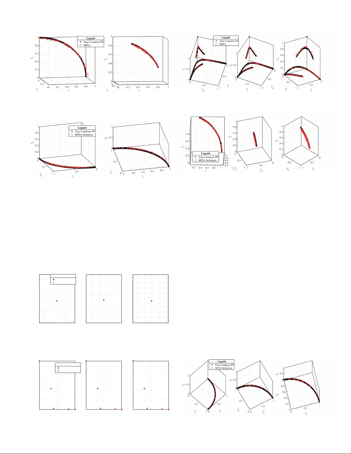
1 A No v el Immune Algorithm for Multiparty Multiobjecti v e Optimization K esheng Chen, W enjian Luo, Senior Member , IEEE , Qi Zhou, Y ujiang liu, Peilan Xu, Member , IEEE Y uhui Shi, F ellow , IEEE Abstract —T raditional multiobjective optimization pr oblems (MOPs) ar e insufﬁciently equipped for scenarios in volving mul- tiple decision makers (DMs), which are pr evalent in many practical applications. These scenarios are categorized as mul- tiparty multiobjective optimization pr oblems (MPMOPs). For MPMOPs, the goal is to ﬁnd a solution set that is as close to the Pareto front of each DM as much as possible. This poses challenges for evolutionary algorithms in terms of searching and selecting. T o better solve MPMOPs, this paper proposes a novel approach called the multiparty immune algorithm (MPIA). The MPIA incorporates an inter-party guided crossov er strategy based on the individual’ s non-dominated sorting ranks from different DM perspectives and an adaptive activation strategy based on the proposed multiparty cover metric (MCM). These strategies enable MPIA to activate suitable individuals f or the next operations, maintain population diversity from different DM perspectives, and enhance the algorithm’s search capability . T o evaluate the performance of MPIA, we compar e it with ordinary multiobjective evolutionary algorithms (MOEAs) and state-of-the-art multiparty multiobjective optimization ev olution- ary algorithms (MPMOEAs) by solving synthetic multiparty multiobjective problems and real-world biparty multiobjective unmanned aerial vehicle path planning (BPU A V -PP) problems in volving multiple DMs. Experimental results demonstrate that MPIA outperforms other algorithms. Index T erms —Multiparty Multiobjective Optimization, Evolu- tionary Algorithm, Immune Algorithm, U A V Path Planning I . I N T R O D U C T I O N Multiparty multiobjecti ve optimization problems (MP- MOPs) pro vide a more effecti ve approach to describing mul- tiobjectiv e optimization problems (MOPs) in volving multiple decision makers (DMs) and each DM is concerned about different conﬂicting objecti ves [ 1 ]–[ 7 ]. In MPMOPs, the goal This study is supported by the National Natural Science Foundation of China (Grant No. U23B2058), Shenzhen Fundamental Research Program (Grant No. JCYJ20220818102414030), the Major Ke y Project of PCL (Grant No. PCL2022A03), Shenzhen Science and T echnology Program (Grant No. ZDSYS20210623091809029), Guangdong Provincial Key Laboratory of Novel Security Intelligence T echnologies (Grant No. 2022B1212010005). (Corr esponding author: W enjian Luo.) Kesheng Chen, W enjian Luo, Qi Zhou and Y ujiang Liu are with Guangdong Provincial K ey Laboratory of Novel Security Intelligence T echnologies, School of Computer Science and T echnology , Harbin Institute of T ech- nology , Shenzhen 518055, China. W enjian Luo is also with Peng Cheng Laboratory , Shenzhen 518000, China. (e-mail: 22s151138@stu.hit.edu.cn, lu- owenjian@hit.edu.cn, 22s051036@stu.hit.edu.cn, 23s151125@stu.hit.edu.cn). Peilan Xu is with School of Artiﬁcial Intelligence, Nanjing Univer - sity of Information Science and T echnology , Nanjing 210044, China. (e- mail:xpl@nuist.edu.cn). Y uhui Shi is with School of Computer Science and Engineering, Southern University of Science and T echnology , Shenzhen 518055, China. (e-mail: shiyh@sustech.edu.cn) The code for this study can be accessed at https://github .com/ MiLab- HITSZ/2023ChenMPIA . is to ﬁnd a solution set as close as possible to the true Pareto front (PF) constructed by the objecti ves of each DM. One practical application of MPMOPs is the unmanned aerial v ehicle (U A V) path planning problems [ 4 ]. U A V path planning problems in urban environments often require con- siderations of multiple objecti ves and inv olve multiple de- partments, such as efﬁcienc y-related departments and safety- related government re gulation departments [ 4 ], [ 8 ]. The efﬁcienc y-related DM focuses on minimizing U A V ﬂying time, reducing energy consumption, and achieving high-quality mis- sion completion (e.g., capturing clear remote sensing photos and collecting extensi ve sensor data) and other efﬁcienc y- related considerations. On the other hand, the safety-related DM aims to minimize external impacts caused by UA Vs, such as minimizing risks to people and vehicles in urban areas, minimizing property damage, reducing noise emissions from U A Vs, and other safety-related concerns. In such an MPMOP , we need to ﬁnd a Pareto set of path solutions that simultaneously consider the objecti ves of both efﬁcienc y-related DM and safety-related go vernment DM. Therefore, when solving MPMOPs, the algorithm is usually required to effecti vely balance the conv ergence and div ersity of the population from multiple DM perspecti ves. Due to the inability of ordinary MOEAs to effecti vely identifying the more valuable solutions and the strategy of maintaining population diversity across dif ferent DMs, ordinary multiob- jectiv e e volutionary algorithms (MOEAs) cannot be directly and effecti vely used to solve MPMOPs. T o efﬁciently solve MPMOPs, such as biparty multiobjec- tiv e U A V path planning problems, some multiparty multiobjec- tiv e e volutionary algorithms (MPMOEAs) [ 1 ]–[ 7 ] hav e been proposed. Some algorithms utilize the non-dominated sorting method from multiple decision maker perspectives to improve the conv ergence ability of the algorithm toward different deci- sion makers (DMs). For example, the ﬁrst MPMOEA, OptMP- NDS [ 1 ], employs the multiparty non-dominated sorting (MP- NDS) operator , which uses the ordinary Pareto sorting ranks of different DMs to calculate the multiparty ranks. Additionally , the MPNDS2 operator, which uses two round ordinary Pareto sort and its corresponding OptMPNDS2 algorithm [ 2 ] hav e been proposed. Following these work, some researchers have designed algorithms with stronger search capabilities using advanced search operators or other ev olutionary algorithm framew orks, such as OptMPNDS3 [ 6 ], MOEA-D/MP [ 7 ], BPNNIA [ 4 ], BPHEIA [ 4 ], BP AIMA [ 4 ]. Howe ver , existing MPMOEAs still face certain limitations when addressing MPMOPs. These limitations can be summa- 2 rized into two main issues: search direction and population div ersity in the presence of multiple DMs. The ﬁrst issue concerns the search direction about con- ver gence. MPMOPs require that the ﬁnal solution set be as close as possible to the true Pareto front constructed by the objectiv es of each DM, which is more stringent than traditional MOPs. Furthermore, at least two or more decision makers, each typically having two or more objecti ves, results in a larger objective space, which reduces the efﬁcienc y of traditional search methods in ﬁnding individuals that meet the requirements. This issue poses a challenge in determining the appropriate search direction. Even though existing MPMOEAs [ 1 ]–[ 7 ] have been improved ov er traditional MOEAs, their performance gains mostly come from specialized sorting tech- niques for MPMOPs or advanced search methods previously used in MOEAs. These works still do not exploit certain inher- ent properties in MPMOPs, such as con ver gence information and div ersity information of the population from different DM perspectiv es. These works only consider relev ant indicators in the function space consisting of all objectives. T o leverage this characteristic, this paper proposes an adap- tiv e operator that combines a novel operator called inter - party guided crosso ver with multiple ordinary operators. In- spired by the guide mechanisms [ 9 ]–[ 11 ] or transfer learning mechanisms [ 12 ]–[ 16 ] in dynamic multiobjective optimization problems (DMOPs), we believe the presence of multiple decision makers allows for the effecti ve application of such an inter-party guided strategy to guide MPMOEAs in their search processes. During the solving process, the population’ s non- dominated sorting ranks are assigned based on the perspectiv es of different decision makers. This information about ranks could be ef fectiv ely utilized to guide search direction. This strategy enables the algorithm to intelligently incorporate information from dif ferent decision makers when selecting crossov er indi viduals, thus enhancing its searchability . The second issue relates to population diversity for different DMs. In MPMOPs, some individuals are at the PF or objectiv e space boundary of a single DM, which may play important roles in maintaining population div ersity for some DMs and rev ealing search direction. Current MPMOEAs, whether using selection operators (in genetic-based algorithms) or activ ation operators (in immune-based algorithms), do not adequately consider these potentially valuable individuals. Experimental results of this paper show that the ordinary selection operators or activ ation operators used in e xisting MPMOEAs hav e limitations in solving MPMOPs. For example, the ﬁxed-size activ ation strategy used in MPMOEAs such as BPNNIA [ 4 ], BPHEIA [ 4 ], and BP AIMA [ 4 ], when combined with existing multiparty non-dominated ranking methods, often results in a lack of di versity for some DMs, which could constrain the algorithm’ s performance. In order to address this issue, we utilize the multiparty cov er metric (MCM) to measure the di versity of the so- lution set across multiple DM’ s perspectives. Furthermore, we hav e designed an adaptiv e activ ation strategy that adjusts the acti vation size based on MCM. This strategy aims to improv e the overall performance of the immune algorithm in solving MPMOPs. By considering the multiparty cov er ratio, our method enhances the diversity of the solution set and effecti vely improv es the performance of the MPMOEA in tackling complex multiparty multiobjectiv e optimization problems. Building upon these strategies, we present a ne w multiparty multiobjectiv e e volutionary algorithm called the multiparty immune algorithm (MPIA) speciﬁcally designed for MP- MOPs. T o assess the effecti veness of MPIA, comprehensiv e experiments are conducted on both multiparty multiobjectiv e benchmarks [ 1 ] and biparty multiobjective U A V path planning problems [ 4 ]. Therefore, the main work of this paper is as follo ws: 1) In order to address the challenge of efﬁciently searching for solutions that meet the requirements of MPMOPs, this paper fully exploits the inherent properties of MP- MOPs and proposes the inter -party guided strategy that effecti vely utilizes population information in the objec- tiv e spaces from different decision makers (DMs). This strategy allows for the intelligent selection of crossover individuals, ultimately enhancing the algorithm’ s effec- tiv eness for MPMOPs. 2) In order to address the issue of loss of population div ersity for some DMs in solving MPMOPs, this paper proposes an adaptiv e activ ation strategy based on the multiparty cover metric (MCM). This strategy guaran- tees that the activ ation set has good diversity for all DMs, thus enhancing the algorithm’ s performance in solving MPMOPs. 3) Building upon the above strategies, a nov el multiparty multiobjectiv e immune algorithm (MPIA) is introduced. Its performance is compared with ordinary multiobjec- tiv e optimization algorithms and state-of-the-art mul- tiparty multiobjectiv e optimization algorithms, includ- ing OptMPNDS, OptMPNDS2, BPNNIA, BPHEIA, and BP AIMA. Experiments are conducted and analyzed on synthetic multiparty multiobjectiv e problems and real- world biparty multiobjecti ve U A V path planning prob- lems. The structure of this paper is as follows: Section II provides an overvie w of MPMOPs and biparty multiobjective UA V path planning problems. This is followed by Section III , which presents a nov el multiparty immune algorithm designed for MPMOPs. Section IV outlines the metrics used and the parameter settings of the algorithms. Next, Section V details the experiments conducted on synthetic multiparty multiob- jectiv e problems, and Section VI e xpands on the experiments in volving biparty multiobjective U A V path planning problems. Finally , we conclude and summarize the paper in Section VII . I I . B AC K G RO U N D S A N D R E L A T E D W O R K This section brieﬂy revie ws the multiparty multiobjectiv e optimization problems and the biparty multiobjectiv e U A V path planning problem. A. Multiparty Multiobjective Optimization Pr oblems A multiobjective optimization problem (MOP) [ 17 ] is con- sidered a problem with multiple conﬂicting objecti ves. W ithout 3 loss of generality , a minimized MOP can be deﬁned as follows. min F ( x ) = ( f 1 ( x ) , f 2 ( x ) , . . . , f m ( x )) , s.t.      g i ( x ) ≤ 0 , i = 1 , . . . , n g h j ( x ) = 0 , j = 1 , . . . , n h x ∈ [ x min , x max ] d , (1) where g i ( x ) denotes the i -th inequality constraint on x , h j ( x ) denotes the j -th equality constraint on x , n g and n h correspond to the numbers of inequality constraints and equality constraints, respectiv ely . x = ( x 1 , x 2 , . . . , x d ) is an d -dimensional decision variable. The parameter m denotes the number of objectiv es, f i ( x ) is the i -th objectiv e function. For two decision vectors x and y satisfy the following two conditions, it can be said that x Pareto dominates y , which is denoted as x ≺ y . 1) none of the objecti ves of x are greater than the objecti ves of y ; 2) there exists at least one objective of x that is less than the corresponding objectiv e of y . Based on the deﬁnition of Pareto dominance, the solu- tion x P is Pareto optimal if and only if no other solutions Pareto dominate x P . In addition, all Pareto optimal solutions compose the Pareto optimal set (PS), and the corresponding objectiv e vectors set is called the P areto front (PF). In MOPs, there is only one DM and the DM is concerned with all the objecti ves. Howe ver , dif ferent objecti ves may be considered by different departments in many real-world applications. For e xample, U A V urban path planning [ 4 ], power ﬂow optimization [ 6 ], and airport slot scheduling may in volve multiple departments or companies. MPMOPs can better describe such problems [ 1 ], where multiple decision makers (DMs) are inv olved, each DM represents a department, and at least one DM cares about multiple objectives. Suppose the objective set of the k -th DM is M k , which rep- resents the set of objecti ves of interest to the k -th DM, which is at least one objecti ve and the objecti ve values of indi vidual x at the k -th DM can be denoted as F k ( x ) = { f i ( x ) | f i ( x ) ∈ M k } . An MPMOP that minimizes all objectiv es can be described as follows [ 1 ]. min E ( x ) = ( F 1 ( x ) , F 2 ( x ) , . . . , F K ( x )) , w here            F 1 ( x ) = { f 11 ( x ) , f 12 ( x ) , . . . , f 1 m 1 ( x ) } F 2 ( x ) = { f 21 ( x ) , f 22 ( x ) , . . . , f 2 m 2 ( x ) } . . . F K ( x ) = { f K 1 ( x ) , f K 2 ( x ) , . . . , f K m K ( x ) } , s.t.      g i ( x ) ≤ 0 , i = 1 , . . . , n g h j ( x ) = 0 , j = 1 , . . . , n h x ∈ [ x min , x max ] d , (2) where E ( x ) is the set of objectiv e vectors from all the K DMs in the MPMOP . The parameter m k denotes the number of objectives considered for the k -th DM. In some cases, a multiparty multiobjecti ve optimization problem can be thought of as a grouping of objectiv e functions (not in the strict sense of grouping, as the objective functions of interest to different decision makers can ov erlap) for the MOP or MaMOP problem combined with information about the decision makers present in the real-world application. W e use x ≺ k y to denote that the decision vector x Pareto dominates of the decision vector y in the objectiv e space F k ( x ) of the k -th DM [ 1 ]. The objectiv e of solving an MPMOP is to search for solutions that are as close to the Pareto front in the objectiv e space of each DM as possible. In addition, x M P is called the multiparty non-dominated Pareto solution, if there does not exist a decision vector z such that [ 5 ]: 1) for at least one party i , z ≺ i x M P ; 2) for any other party j , z ≺ j x M P , or z and x M P are non-dominated for each other . The main difference between MPMOPs and MOPs is that they introduce multiple DMs, which means that the PS of MPMOPs must be their own from the perspectiv e of multiple DMs. MOPs ov erlook this widely present requirement in real- world applications. Therefore, if we directly use optimization algorithms designed for multiobjecti ve optimization problems (MOPs) or many-objectiv e optimization problems (MaOPs), they will not effecti vely differentiate between x P and x M P , resulting in the solution set that cannot be simultaneously con- sidered by multiple decision makers (DMs), and the guarantees of conv ergence and di versity cannot be provided [ 1 ]–[ 7 ]. It is notew orthy that the core motiv ation of MPMOPs lies in collaborati ve decision making by dif ferent DMs using a completely consistent population of solutions. Unlike in multitask problems (MTPs) [ 18 ] or multiobjective multi-task problems (MOMTPs) [ 19 ], where dif ferent tasks can have their populations that may not reside in the same decision variable space (e.g., different numbers of decision variables), in MPMOPs, the set of candidate solutions considered must be identical from all DMs’ perspectives. Based on this shared set of candidate solutions, optimization is carried out according to the different objectiv es of the DMs. B. Biparty Multiobjective UA V P ath Planning Pr oblem U A Vs hav e gained widespread usage in various urban opera- tions, including aerial photography [ 20 ], unmanned deliveries [ 21 ], urban trafﬁc monitoring [ 22 ], and IoT data collection [ 23 ]. Considering these applications, some univ ersal biparty multiobjectiv e U A V path planning problems (BP-UA VPPs) which inv olve the objecti ves for efﬁcienc y-related DM, the objectiv es for safety-related DM, and the constraints in U A V path planning are constructed [ 4 ]. Here, a brief introduction is given. The problems consist of two decision makers, the ef ﬁciency decision maker and the safety decision maker . The ef ﬁciency decision mak er considers objectiv es regarding path length, ﬂight energy consumption, path height changes, and mission hov er point distance and the safety decision maker considers the objectiv es on fatal risks, property risks, and noise pollution. These objectives are computed based on the given maps (in this paper , two maps called MAP-A and MAP-B are considered) and the giv en path ( x ) of the U A V . For a gi ven path consisting of n +1 trajectory points, where the i -th discrete trajectory 4 point can be expressed as  p i = ( x i , y i , z i ) , the decision vector x corresponding to the given path can be expressed as x = ( x 0 , y 0 , z 0 , x 1 , y 1 , z 1 , . . . , x n , y n , z n ) . Based on the path trajectory points of the U A V , we can easily calculate the objectiv e values for efﬁcienc y decision maker and safety deci- sion maker . The detailed formulas and methods for calculating these objectiv es are giv en in Appendix S–B “Details about Biparty Multiobjective U A V P ath Planning Problems” . Based on the abov e-mentioned different decision makers with different objectiv es, we further formulate the problem. The efﬁcienc y objectiv es include the minimization of ﬂight path length f length , the minimization of ﬂight energy consump- tion f fuel , the minimization of path height changes f height and minimization of the total sum of mission hover point distance f distance . The safety objectives include the minimization of fatal risks f fatal , the minimization of property risk f eco and the minimization of noise pollution f noise . Without loss of gen- erality , the model for all cases can be represented generically as follows [ 4 ]. min ( F eff ( x ) , F safe ( x )) , F eff = ( f length ( x ) , f distance ( x ) , . . . ) , F safe = ( f fatal ( x ) , f eco ( x ) , . . . ) , x = ( x 0 , y 0 , z 0 , x 1 , y 1 , z 1 , . . . , x n , y n , z n ) , s.t.      H min ≤ z i ≤ H max , i = 1 , . . . , n ; | α i | ≤ α max , i = 1 , . . . , n − 1; | β i | ≤ β max , i = 1 , . . . , n − 1 . (3) where F eff is the set of objecti ves for the ef ﬁciency DM, and F safe is the set of objectives for the safety DM. Here, we construct twelve cases for the experiment. The details of all cases will be gi ven in Section VI . I I I . P RO P O S E D A L G O R I T H M This section introduces the motiv ation behind the proposed strategies and an o vervie w of the multiparty immune algorithm (MPIA). Subsequently , the details of the multiparty non- dominated sorting operation, adapti ve acti vation operation, clone operation, and adapti ve operator are presented. A. Motivations and Overview 1) Motivation of Inter-party Guided Crosso ver: MPMOPs typically inv olve two or more decision makers, each with two or more objectives. At the same time, MPMOPs require that the solution set is as close to the corresponding true Pareto front of each DM as possible, which is more stringent than traditional MOPs. It poses a challenge in determining the appropriate search direction and obtaining suitable individu- als. Existing MPMOEA algorithms, such as OptMPNDS [ 1 ], OptMPNDS2, MOEA-D/MP [ 5 ], [ 7 ], OptMPNDS3 [ 6 ], and BP AIMA [ 4 ], have been proposed in recent years. Howe ver , these improv ements are mainly attributed to the use of multiparty non-dominated sorting methods designed for MPMOPs or more advanced search methods that have been used in ordinary MOEAs. These studies do not fully utilize the guiding information inherent in the objective space of multiple DMs and can improv e the search direction to the Pareto front of some DMs. Reasonably utilizing this guiding information can effecti vely enhance the search capability of the algorithms. Such an idea has been widely applied in dynamic mul- tiobjectiv e optimization problems (DMOPs) and is referred to as guide mechanisms [ 9 ]–[ 11 ] or transfer learning mech- anisms [ 12 ]–[ 16 ]. F or instance, Jiang et al. [ 16 ] proposed an individual-based transfer learning algorithm for DMOPs, utilizing historical search information to guide population re- initialization. Drawing inspiration from such work, we believ e that multiparty multiobjecti ve optimization algorithms could lev erage the con ver gence information of individuals across different DMs. Indi viduals close to at least one DM’ s PF can guide the population to generate individuals approaching both DMs’ PF . Therefore, we have designed a crossover operator based on the inter-party guided crossov er strategy . This strategy intel- ligently selects guiding individuals for the guided indi vidual based on the individual’ s non-dominated ranks from dif ferent DM perspectives. W e giv e an example in Fig. 1 for better understanding. Suppose we consider an MPMOP with two decision makers, i.e., DM1 and DM2, and each considering two different decision objectives, totaling four objectives. The population under DM1’ s perspectiv e is shown in Fig. 1 (a), and the population under DM2’ s perspective is sho wn in Fig. 1 (b). The hexagonal individuals will serve as the guided individuals, while the circular individuals will serve as the guiding individuals. This strategy aims to search for ne w individuals located at the current PF of both DMs. The ﬁgure illustrates the fundamental concept of the proposed inter-party guide crossover . The details will be gi ven in Section III-E . 𝒇 𝟏 𝒇 𝟑 𝒇 𝟒 𝒇 𝟐 (a ) V iew of DM1 (b) V iew of D M2 P F o f DM1 P F o f DM2 P S f o r M P M O P P S f o r M OP Fig. 1. An example of using inter-party guided crossover . The black circular entities are located on the PF of both DMs. The hexagonal entities are re garded as individuals being guided, while the black circular entities serve as guiding individuals, enabling crossover with the expectation of generating offspring that approach all PF of different DMs. Additionally , using this approach in solving MPMOPs has more intuitiv e advantages than using it in solving MOPs. In MOPs in volving single DM, guiding information is typically provided by a select few individuals near the front. Thus, the population conv erges towards these guiding individuals. W ith- out proper strategic control, the population may experience potential local con vergence and lack of div ersity . Howe ver , in multiparty multiobjective optimization problems, guidance is required only from the perspecti ve of one DM, leading to 5 T ABLE I T H E S I T UAT I O N O F T H E S O L U T I O N S F R O M D I FF E R E N T P E R S P E C T I V E S Solution Layers * PS for DM1 PS for DM2 PS for MOP PS for MPMOP X 1 (1,1) ✓ ✓ ✓ ✓ X 2 (1,1) ✓ ✓ ✓ ✓ X 3 (1,1) ✓ ✓ ✓ ✓ X 4 (1,2) ✓ × ✓ × X 5 (1,3) ✓ × ✓ × * Non-dominated layers from different DM perspectiv es a signiﬁcant increase in the number of individuals capable of offering guiding information. As a result, in multiparty multiobjectiv e optimization problems, most of the population could consist of individuals capable of pro viding guiding information based on this strategy . 2) Motivation of Adaptive Activation: In MOPs, some individuals near the boundary (at least one objectiv e of the achiev es minimum value for the whole PS or the corre- sponding DM) of a single DM must be individuals at the Pareto non-dominated set (because only one DM in ordinary MOPs). Howe ver , in MPMOPs, this situation is not always true. Suppose we get the ﬁv e solutions { x 1 , x 2 , x 3 , x 4 , x 5 } and the information corresponding to solutions is shown in T able I . The individuals { x 1 , x 2 , x 3 } marked black in Fig. 2 constitute the multiparty common PS. The other solutions are non-common PS, but they may still be individuals at the Pareto front or boundary of a single DM. This is because the algorithm uses multiparty non-dominated sorting operations such as the MPNDS operator or the MPNDS2 operator , which makes it possible that some individuals at the boundary of objectiv e space may not be at the multiparty Pareto set. 𝒇 𝟏 𝒇 𝟑 𝒇 𝟒 𝒇 𝟐 𝑥 1 𝑥 2 𝑥 3 𝑥 4 𝑥 5 𝑥 5 𝑥 4 𝑥 3 𝑥 2 𝑥 1 ( a) V i ew of D M1 ( b) V i ew of D M2 ex is ti n g activ ation m o r e id ea l a ctiv atio n id ea l sear ch d ir ec tio n ex is tin g s ea r ch d ir ec tio n P S f o r M P M O P (f o r a ll DMs) P F co r r esp o n d in g to DM Fig. 2. Inappropriate activ ations cause the population to lose diversity in the DM1 perspective. The existing method will select { x 1 , x 2 , x 3 } as the activ ation set. Howe ver , adding x 4 enables the activation set to hav e higher population diversity for both DMs. These individuals, such as { x 4 , x 5 } in Fig. 2 and table I , which are located only in the PF of the corresponding DMs from the perspective of partial DMs are the main contributors to the population div ersity for these DMs and play important roles in guiding search. Methods that solely consider the common frontier individuals (PS for MPMOP) hav e to some extent compromised the long-term diversity of the entire population. Unfortunately , existing MPMOEAs directly select a ﬁxed number of indi viduals from a common P areto front. As a result, these algorithms fail to maintain diversity among offspring across different DM objecti ve spaces. They also struggle to effecti vely utilize individuals located on the Pareto front (PF) in certain DM objecti ve spaces to produce of fspring, despite the valuable information the y contain. T o better understand this issue, we present a comparison of the real performance of the existing multiparty immune algorithms such as BP AIMA, etc., and our proposed MPIA. Fig. 28 illustrates that when using the existing multiparty immune algorithm to activ ate individuals, although most of these individuals are located on the common PF of both DMs, they fail to represent the population information of DM1. In contrast, Fig. 29 presents the more ideal activ ated individuals (selected from the population to produce offspring), where the activ ated indi viduals cover the fronts of different DMs. In appendix S–C “Analysis and V isualization of the Impact of Activation Size” , we provide a more detailed analysis of the activ ation size. 8000 8500 9000 9500 10000 400 600 800 1000 1200 1400 0.04 0.045 0.05 0.055 0.0 6 0.1 0.2 0.3 0.4 0.5 0.6 Inactive Activating (BPNNIA, BPHEIA and BPAIMA) Fig. 3. The population distribution in solving Case 1 using existing multiparty immune algorithms (such as BPNNIA, BPHEIA and BP AIMA) is sho wn when the number of activ ations is set to 20. The Case 1 problem is giv en in T able VII . 8000 8500 9000 9500 10000 400 600 800 1000 1200 1400 0.04 0.045 0.05 0.055 0.06 0.1 0.2 0.3 0.4 0.5 0.6 Inactive Activating (the more ideal method) Fig. 4. The population distribution in solving Case 1 using MPIA is shown when the number of activ ations is adaptive. The Case 1 problem is given in T able VII . If the adaptive strategy for selecting the appropriate number of activ ated individuals can ensure div ersity from multiple perspectiv es, it will effecti vely enhance the performance of 6 immune algorithms when addressing MPMOPs. Based on this motiv ation, we hav e proposed the multiparty cover metric (MCM) to measure the diversity quality of the selected acti- vated individuals, thus further enabling the adaptiv e activ ation strategy in algorithm design for solving MPMOPs. The details will be giv en in Section III-C . 3) Overview of Pr oposed Algorithm: Based on the above motiv ations, this paper designed a novel immune optimization algorithm for MPMOPs. Fig. 5 shows the main process of one iteration in MPIA, as shown in Alg. 1 . The ﬁrst subﬁgure describes population distributions in the objectiv e space of different DMs’ vie w . The operation (a), i.e., MPNDS2 (Alg. 2 ) sorts the population to get the multiparty multiobjectiv e non- dominated ranks. The operation (b), i.e., adapti ve activ ation (Alg. 4 ) is used to select the good individuals for both DMs as the parent indi viduals to produce offspring. The operation (c), i.e., cloning operation (Alg. 5 ), uses the non-dominated sorting rank information and crowding distance information [ 17 ] to allocate replication resources. The operation (d), i.e., Alg. 6 is the adapti ve operation based on the multiple DE operator and inter-party guided crossover operator . The operation (e), i.e., Alg. 3 uses multiparty non-dominated sorting and cro wding distance to select the population into the next iteration. B. Multiparty Nondominated Sorting and Selection The multiparty non-dominated sorting operator is designed for MPMOPs to select solutions that closely approximate the Pareto non-dominated front of multiple DMs. In the proposed algorithm, we employed the MPNDS2 operator [ 2 ] to conduct multiparty non-dominated sorting. The MPNDS2 operator [ 2 ] utilizes two rounds of fast non-dominated sorting for multiparty non-dominated sorting. The ﬁrst round in volv es non-dominated sorting from the perspectiv e of each DM, as depicted in lines 2-4 of Alg. 2 . The second round entails a non-dominated sort based on the number of non-dominated layers of each DM. The resulting number of layers determines the order of the multiparty non-dominated sort. This approach ensures that indi viduals ranked at the top by multiple DMs also occupy top positions in the multiparty non-dominated sorting rank of individuals. For the selection operator, this is the same step as most multiparty multiobjecti ve optimization e volutionary algorithms (MPMOEAs) such as OptMPNDS2 [ 2 ] and BP AIMA [ 4 ]. First, we retain the solutions based on the number of layers of multiparty non-dominated sorting operator MPNDS2 layer by layer, as shown in lines 1-6 in Alg 3 . In a giv en layer , if the total number of retained solutions exceeds the number of maintained population, the crowding distance information ﬁlters out some of the cro wded solutions in that layer , as shown in lines 7-9 in Alg 3 . C. Adaptive Activation The activ ation operator in immune algorithms is designed to select a certain percentage of high-quality individuals from the population to clone and generate improved individuals. T raditional immune algorithms, such as NNIA [ 24 ], HEIA [ 25 ], AIMA [ 26 ], as well as multiparty immune algorithms like BP AIMA [ 4 ], commonly employ a ﬁxed number of individuals from the Pareto front as acti ve indi viduals in subse- quent cloning and cross-mutate steps. Howe ver , this ﬁxed-size activ ation strategy could result in a loss of div ersity when addressing MPMOPs. T o tackle this problem, a numerical value known as the multiparty cover metric (MCM) is used to ev aluate the performance of different sets of activ e individuals. Before calculating the MCM, it is necessary to calculate the cov er metric ( cm ) for the different decision makers. The cover metric ( cm k ) for the k -th DM is calculated using the following formula. cm k = min i ∈ M k  max( f i ( A )) − min( f i ( A )) max( f i ( B k )) − min( f i ( B k ))  , (4) where the function f i ( · ) represents a list of the i -th objective value components of the corresponding indi vidual set. A represents the giv en activ ated individuals, and B k is the set composed of some indi viduals located at the Pareto front of the k -th DM among all individuals. M k denotes the set of objectiv es for the k -th DM. Fig. 6 visually illustrates the concept of coverage metrics. After calculating the cover metrics cm for all DMs, the smallest cm is chosen as the indicator to measure the quality of the gi ven activ ation individual set. This indicator is called the multiparty co ver metric ( M C M ), and its calculation formula is as follows. M C M = min k =1 ,...,K cm k , (5) where cm k is the cov er metric of the k -th DM, and K is the number of decision makers. The M C M measures the proportion of the P areto front distribution range for a giv en activ ation individual set A from the worst-case DM’ s perspectiv e. A higher value of M C M indicates better di versity for all DMs in the gi ven activ ation individual set A . Algorithm 4 Adapti veActi vation Input: P t (the sorted population in the t -th iteration) Output: A (the acti v ated indi vidual set) 1: Activ ateN umList = { 20 , 30 , 40 , 50 , 60 , 70 } ; 2: Calculate the B k (PS for k -th DM, Refer to Fig. 6 ) 3: for i ∈ { 1 , · · · , | Activ ateN umList |} do 4: nA = Activ ateN umList [ i ] ; // Set the i -th list element as the size of acti vation individual set A . 5: A = P t [1 : nA, :] ; 6: for k ∈ { 1 , · · · , K } do 7: Calculate cm k according to Eq. 4 based on A , B k .; 8: end for 9: Calculate M C M according to Eq. 5 based on cm k .; 10: if M C M > 0 . 99 then 11: break ; 12: end if 13: end f or By computing the M C M of a gi ven acti vation individual set A , we can quantify the diversity of A for dif ferent DMs. The 7 4 3 2 1 𝒇 𝟏 𝒇 𝟐 𝒇 𝟑 𝒇 𝟒 V i ew o f D M 2 V i ew o f D M 1 (a ) M P N D S2 no n - do m i na ted l a y ers o f D M 1 no n - do m i na ted l a y ers o f D M 2 1 2 3 4 5 (b) A da pti v e A cti v a ti o n (c) C l o ning V i ew o f D M 2 V i ew o f D M 1 ra nd / 1 / b i n D E Ope r a t o r (C R =0 . 5 , F = 0 .5 ) (d.2) I nter - pa rty Gui ded SBX Opera to r V i ew o f D M 2 V i ew o f D M 1 ra nd/ 2 / bi n DE Ope ra to r (CR = 0 .9 , F=0 .7 ) O n th e PF o f b o t h D M’ s v i ew In s u f fi ci en t conve r g en ce i n t h e v i ew o f o n e D M (d) A d apt i v e Ope r at or Ba s ed o n di ffer ent s ea r ch s ta g es a nd n on - do m i na ted l a y ers of bo th D M s . (e) S ele ctio n (e) S el ec tion (d.1) D E Opera to rs A cti v a ti o n ba s e o n m ul ti pa rty cover m etri c 𝒇 𝟏 𝒇 𝟐 𝒇 𝟑 𝒇 𝟒 𝒇 𝟏 𝒇 𝟐 𝒇 𝟑 𝒇 𝟒 Fig. 5. Overall framework of the MPIA. Here, for better understanding, we assume that there are two parties and each party has two objectives. Algorithm 1 MPIA Input: nC (the clone size, and also the population size) Output: M P S (the multiparty Pareto optimal solutions) 1: t = 0 , P 0 = Initialization ( nC ) # Initialize population P 0 using a uniform distrib ution ; 2: E 0 = Evaluation ( P 0 ) # Calculate the objective values for differ ent DMs E 0 of the population P 0 . ; 3: P 0 = MPNDS2 ( P 0 , F 0 ) # Sort the population P 0 for MPMOPs using Alg . 2 . ; 4: while F E is not reached do 5: A = AdaptiveActi vation ( P t ) # Generate activation set A from population P t using Alg. 4 . ; 6: C = Clone ( A , nC ) # Generate clone individual set C fr om activation set A using Alg. 5 . ; 7: O = AdaptiveOperator ( P t , A , C , t ) # Generate of fspring O fr om clone individual set C and P t using Alg. 6 . ; 8: P t = P t ∪ O # Combine population P t and offspring O ; 9: E t = E t ∪ Evaluation ( O ) # Combine objective values of population and objective values of of fspring. ; 10: B = OptMPNDS2 ( P t , E t ) # Sort the ne w population P t using Alg. 2 . ; 11: P t +1 = Selection ( B , nC ) # Select individual set P t +1 fr om the sorted population B using Alg. 3 . ; 12: t = t + 1 13: end while 14: Set M P S as solutions which are Pareto optimal in all DMs in P t +1 ; algorithm aims to select an activ ated individual set A with a high value of the M C M to maintain sufﬁcient diversity of the offspring. This is easily achiev able because as the size of the activ ation individual set A increases, the M C M always mono- tonically increases. Ho wev er , an excessi vely large activ ation individual set A can cause the algorithm to struggle to ef fec- tiv ely distinguish more conv ergent individuals for MPMOPs, thus compromising the algorithm’ s conv ergence performance for MPMOPs. A threshold value (e.g., 0.99) is set to strike a balance. The minimum number of activ ations, which ensures M C M is no smaller than the threshold value, is selected from a candidate activ ation number list Activ ateN umList (e.g., { 20 , 30 , 40 , 50 , 60 , 70 } ). The pseudocode for this strategy is shown in Alg. 4 . D. Clone The cloning operator is a vital component of the immune algorithm [ 4 ], [ 24 ], [ 26 ]–[ 29 ] that facilitates the allocation of computational resources. Assigning more replication resources to the activ ation individuals with higher quality , increases their opportunities to cross-mutate and generate offspring. In many 8 𝑓 1 C onsi der on objec t i ve 𝒇 𝟏 𝑓 2 𝐦𝐚𝐱 𝒇 𝟏 𝑨 − 𝐦𝐢 𝐧 ( 𝒇 𝟏 ( 𝑨 ) ) 𝐦𝐚𝐱 𝒇 𝟏 𝑩 𝟏 − 𝐦𝐢 𝐧 𝒇 𝟏 𝑩 𝟏 𝑥 1 𝑥 2 𝑥 3 𝑥 4 𝑥 5 𝑓 1 𝑓 2 𝐦𝐚𝐱 𝒇 𝟐 𝑨 − 𝐦𝐢 𝐧 ( 𝒇 𝟐 ( 𝑨 ) ) 𝐦𝐚𝐱 𝒇 𝟐 𝑩 𝟏 − 𝐦𝐢 𝐧 𝒇 𝟐 𝑩 𝟏 𝑥 1 𝑥 2 𝑥 3 𝑥 4 𝑥 5 C onsi der on objec t i ve 𝒇 𝟐 𝑓 3 𝑓 4 𝐦𝐚𝐱 𝒇 𝟑 𝑨 − 𝐦𝐢 𝐧 𝒇 𝟑 𝑨 𝐦𝐚𝐱 𝒇 𝟑 𝑩 𝟐 − 𝐦𝐢𝐧 𝒇 𝟑 𝑩 𝟐 𝑥 1 𝑥 2 𝑥 3 𝑥 4 𝑥 5 C onsi der on objec t i ve 𝒇 𝟑 𝑓 4 𝐦𝐚𝐱 𝒇 𝟒 𝑨 − 𝐦𝐢𝐧 𝒇 𝟒 𝑨 𝐦𝐚𝐱 𝒇 𝟒 𝑩 𝟐 − 𝐦𝐢 𝐧 𝒇 𝟒 𝑩 𝟐 𝑥 1 𝑥 2 𝑥 3 𝑥 5 C onsi der on objec t i ve 𝒇 𝟒 𝑓 3 𝒄 𝒎 𝟐 = 𝐦𝐢 𝐧 ( 𝐦𝐚𝐱 𝒇 𝟑 𝑨 − 𝐦𝐢 𝐧 𝒇 𝟑 𝑨 𝐦 𝐚𝐱 𝒇 𝟑 𝑩 𝟐 − mi n 𝒇 𝟑 𝑩 𝟐 , 𝐦𝐚𝐱 𝒇 𝟒 𝑨 − 𝐦𝐢 𝐧 𝒇 𝟒 𝑨 𝐦 𝐚𝐱 𝒇 𝟒 𝑩 𝟐 − 𝐦𝐢𝐧 𝒇 𝟒 𝑩 𝟐 ) 𝒄 𝒎 𝟏 = 𝐦𝐢 𝐧 ( 𝐦 𝐚𝐱 𝒇 𝟏 𝑨 − 𝐦𝐢 𝐧 𝒇 𝟏 𝑨 𝐦𝐚𝐱 𝒇 𝟏 𝑩 𝟏 − 𝐦𝐢 𝐧 𝒇 𝟏 𝑩 𝟏 , 𝐦𝐚𝐱 𝒇 𝟐 𝑨 − 𝐦𝐢 𝐧 𝒇 𝟐 𝑨 𝐦 𝐚𝐱 𝒇 𝟐 𝑩 𝟏 − 𝐦𝐢 𝐧 𝒇 𝟐 𝑩 𝟏 ) < (a) V iew of DM 1 (b) V iew of DM 2 𝑥 4 Fig. 6. The rele vant details of calculating the cov er metric cm k of the k -th DM for the given activation individual set A = { x 1 , x 2 , x 3 } . The details about the population are provided in T able I . Where B k is the set of frontier individuals for k -th DM. M k denotes the set of objectives for the k -th DM. M 1 = { f 1 , f 2 } , M 2 = { f 3 , f 4 } , B 1 = { x 1 , x 2 , x 3 , x 4 , x 5 } , B 2 = { x 1 , x 2 , x 3 } . The ﬁgure intuitiv ely demonstrates why the cover metric cm indicator can measure the cover metric of activ ation individual set A in different DM perspectiv es. The metric cm 2 is close to 1 and cm 1 is much smaller than cm 2 , indicating that the giv en activation individual set A has sufﬁcient div ersity for DM2, but lacks diversity for DM1. Algorithm 2 MPNDS2 [ 2 ] Input: P t (the population in the t -th iteration), E t = ( F 1 = ( f 11 , f 12 , . . . , f 1 m 1 ) , F 2 = ( f 21 , f 22 , . . . , f 2 m 2 ) , . . . , F K = ( f K 1 , f K 2 , . . . , f K m K )) (the objectiv e v alues of population for different DMs) Output: P t (the sorted population) 1: L = ∅ ; 2: for i ∈ { 1 , · · · , K } do 3: P t , L [: , i ] = NonDominatedSorting ( P t , F i ) ; 4: end f or 5: P t , LL = NonDominatedSorting ( P t , L ) ; Algorithm 3 Selection Input: B (the candidate population sorted by MPNDS2 oper - ator), nC (the number of cloning) Output: P (the selected population) 1: sort B by cro wding distance for each rank. 2: P = ∅ , i = 1 ; 3: while |P | < nC do 4: Add the i − th layer’ s indi viduals into P . 5: i = i + 1 ; 6: end while 7: while |P | > nC do 8: Remov e the least crowded individual in the i -th layer from P . 9: end while immune algorithms, resource allocation is primarily deter- mined by the crowding distance. Howe ver , considering our adaptiv e activ ation strategy , it is possible that some acti vated individuals may not be Pareto solutions for MPMOP . There- fore, maintaining population conv ergence becomes crucial. In order to achie ve this, we utilize the crowding distance during the cloning process and incorporate a con ver gence metric to allocate computational resources ef fecti vely . The conv ergence metric ( p i ) for the i -th activ ated individual is calculated using the following formula. p i = ( max j =1 ,...,nA lay er j ) − l ay er i , (6) where p i represents the conv ergence metric of the i -th acti- vated individual, nA is the number of acti v ated individuals, and lay er i denotes the multiparty non-dominated sorting layers of the i -th activ ated individual. The higher value of p i indicates better conv ergence. Based on p i , the formula for determining the number of clones per individual is as follows: C loneN umList [ i ] = ⌈ nC · CD ( A i ) + p i P nA j =1 ( CD ( A j ) + p j ) ! ⌉ , (7) where C l oneN umList [ i ] represents the number of replicates for the i -th activ ated individual, A i represents the i -th acti- vated indi vidual, CD ( · ) represents the corresponding crowding distance, ⌈·⌉ is a function that rounds up the v alue, and nC represents the desired number of indi viduals to be cloned. Algorithm 5 Clone Input: A (the activ ation individual set), nC (number of clones) Output: C (the clone individual set) 1: Calculate the cloning number list C l oneN umList of per individual based on Eq. 7 2: C = ∅ ; 3: for i ∈ { 1 , · · · , |A|} do 4: for j ∈ { 1 , · · · , C l oneN umList [ i ] } do 5: C = C ∪ A [ i, :] ; 6: end for 7: end f or This method ensures that the MPIA algorithm considers div ersity and sufﬁcient conv ergence during cloning. When all activ ated individuals are on the ﬁrst multiparty non-dominated sorting layer for MPMOPs, this method is equiv alent to 9 ordinary cloning methods. The pseudocode for this strategy is shown in Alg. 5 . E. Adaptive Operator This section introduces two existing dif ferential ev olution (DE) operators and the proposed inter-party guided crossov er used in this algorithm. A set of rules has been designed to ensure the appropriate application of these operators during the algorithm process. Firstly , the ﬁrst operator is employed for cross-mutation with a probability of P 1 . The probability P 1 of using the ﬁrst operator is controlled by the following formula, which is related to the number of iterations. This concept is also applied in AIMA [ 26 ] and BP AIMA [ 4 ]: P 1 = 0 . 95 1 + exp (20 ∗ t T − 3 . 0) , (8) where t represents the number of current generations and T denotes the maximum number of generations. This control method enables the algorithm to search with a large step size in the early stage, accelerating the population’ s conv ergence and enhancing the search capability of the algorithm. First Operator : The rand/2/bin DE operator [ 26 ], [ 30 ] with a large step size primarily enables the algorithm to exhibit a strong search capability in the early stage. op 1 : O i,j =      C i,j + F 1 ∗ ( A r 1 ,j − A r 2 ,j ) if r and < C R 1 or + F 1 ∗ ( A r 3 ,j − A r 4 ,j ) j == r and j C i,j otherwise. , (9) where O represents the offspring individuals generated after the operation, C represents the cloned individuals, and A rep- resents the activ ated indi viduals. The subscripts i, j represent the j -th decision variable of the i -th corresponding individual. Index r 1 , r 2 , r 3 , r 4 are the distinct integers randomly selected from [1 , 2 , . . . , nA ] , nA is the size of activ ated individuals. C R 1 means the crossover rate, which is 0.9. F 1 means the scaling factor , which is 0.7. The algorithm uses the second and third operators with a probability of 1 − P 1 . When the three conditions ( C on 1 , C on 2 , C on 3 ) used by the second operator (inter-party guided crossov er) are held, the algorithm uses the second operator . Otherwise, the algorithm resorts to the third operator . The three conditions ( C on 1 , C on 2 , C on 3 ) for the second operator are as follo ws: C on 1 : The cloned individual (guided individual) is not located at the multiparty non-dominated forefront after sorting with the MPNDS2 operator . This ensures that the re- sulting offspring tend to be positioned at the forefront of multiple decision makers. C on 2 : The ﬁnding in the population (guiding individual) is closer or equally close to the forefront of a DM than the guided indi vidual. Additionally , the multiparty non- dominated rank of the guiding individual is smaller than that of the guided individual. This enables the guiding individual to provide effecti ve information to the guided individual. C on 3 : For all clones of the same guided individuals who hav e not undergone one inter-party guided crossover operation, then use the guided crossover with probability P 2 , which is 0.6. This allows an individual and copy to use multiple different crossover methods to maintain population diversity . Second Operator : The inter-party guided crossov er operator is then performed using the simulated binary crossov er [ 31 ], as shown in the follo wing equation. op 2 : O i,j = ( 0 . 5 ∗ [(1 + δ ) ∗ C i,j + (1 − δ ) ∗ A guide,j ] if r and < P c C i,j otherwise. , (10) where O represents the offspring individuals generated after the operation, C represents the cloned individuals, and A rep- resents the activ ated indi viduals. The subscripts i, j represent the j -th decision variable of the i -th corresponding individual. Index g uide is the index of the guiding individual. P c means the crosso ver rate, which is the reciprocal of decision v ariables. δ is calculated by the follo wing formula [ 31 ]. Third Operator : The commonly used rand/1/bin DE operator [ 26 ], a con ventional crossov er operator that is used when individuals do not fulﬁll the conditions of the ﬁrst and the second approaches. It is a basic crossover . op 3 : O i,j =      C i,j + F 2 ∗ ( A r 1 ,j − A r 2 ,j ) if r and < C R 2 or j == r and j C i,j otherwise. , (11) where C R 2 means the crossover rate, which is 0.5. F 2 means the scaling factor , which is 0.5. After all crossovers, the mutation operation is performed on the individual using the polynomial mutation [ 17 ] (PM) operator . The pseudocode for this strategy is shown in Alg. 6 . Algorithm 6 Adapti veOperator Input: P (the population set), A (the activ ation individual set), C (the clone individual set), t (current iteration number) Output: O (the of fspring set) 1: for i ∈ { 1 , · · · , |C |} do 2: r 1 , r 2 , r 3 , r 4 = RandIndex(); 3: if rand () < P 1 then (Eq. 8 ) 4: O [ i, :] = Operation1 ( C [ i, :] , A [ r 1 , :] , A [ r 2 , :] , A [ r 3 , :] , A [ r 4 , :]); (Eq. 9 ) 5: else 6: Find the guiding individual A g uide for C [ i, :] which meets condition C on 1 & C on 2 from population P ; 7: if exist ( A g uide ) and condition C on 3 hold then 8: O [ i, :] = Operation2 ( C [ i, :] , A g uide ) ; (Eq. 10 ) 9: else 10: O [ i, :] = Operation3 ( C [ i, :] , A [ r 1 , :] , A [ r 2 , :]) ; (Eq. 11 ) 11: end if 12: end if 13: O [ i, :] = PolynomialMutation ( O [ i, :]) ; 14: end f or 10 I V . M E T R I C A N D E X P E R I M E N TA L S E T T I N G S A. Metric For MPMOPs, Liu et al. [ 1 ] used the multiparty in verted generational distance (MPIGD [ 1 ]) to measure the perfor - mance of the algorithms. MPIGD is deﬁned as MPIGD ( P M P , P ) = P v ∈ P M P d ( v , P ) | P M P | , (12) d ( v , P ) = min s ∈ P ( M X j =1 q ( v j 1 − s j 1 ) 2 + · · · + ( v j m j − s j m j ) 2 ) , (13) where P M P represents the true PF of the MPMOP and P is the PF obtained by the algorithms. d ( v , P ) represents the minimum distance between v from P and points from P . Respectiv ely , ( v j 1 , ..., v j m ) means the m objecti ves of the j - th DM for solution v , and ( s j 1 , ..., s j m ) means the same for solution s . Howe ver , there is often no deﬁnite true PF for real-world applications to calculate the MPIGD metric. T o obtain the performance of different algorithms on MPMOPs, in this paper , the sumHV metric is adopted, which is based on the hypervolume (HV) metric [ 4 ], [ 32 ]. For general MOPs, the HV metric is deﬁned as the super volume constituted by the normalized solution set. Suppose H V i is the HV metric of the solution set on the set of objectiv es of the i -th DM, then sumHV is deﬁned as the sum of H V i of the solution set on all decision makers shown as follows. sumHV ( P ) = K X i =1 H V i ( P ) . (14) The sumHV metric examines the performance of the solu- tion set on different decision makers, and the performances of all DMs are chosen as the performance metric of the solution set. B. Experimental Settings The experimental comparison in volv es se veral algorithms, including the ordinary multiobjective algorithm NSGA-II [ 17 ], NSGA-III [ 33 ] and existing multiparty multiobjectiv e opti- mization algorithms such as OptMPNDS [ 1 ] and OptMPNDS2 [ 2 ]. Additionally , multiparty multiobjective optimization al- gorithms framed in an immune algorithm context were also considered, such as BPNNIA [ 4 ] that e xtends from NNIA [ 24 ], BPHEIA [ 4 ] that extends from HEIA [ 25 ], and BP AIMA [ 4 ] that extends from AIMA [ 26 ]. T o comprehensi vely ev aluate MPIA ’ s performance relative to existing multiobjective optimization algorithms and other multiparty multiobjecti ve optimization algorithms, this study designs experiments on synthetic multiparty multiobjective and biparty multiobjectiv e UA V path planning problems. Each experiment is run independently 30 times for all the algo- rithms. T able II sho ws the parameter settings related to the experi- ment, NSGA-II, NSGA-III, and MPMOEAs primarily use the default settings in the PlatEMO platform [ 34 ] or the original paper . NSGA-II, OptMPNDS, OptMPNDS2, BPNNIA, and BP AIMA employ the conv entional simulated binary crossov er (SBX) operator , while MPIA utilizes the guided-based sim- ulated binary crossover operator . All these algorithms also employ the polynomial mutation operator . BPHEIA uses the rand/1/bin DE operator-I, BP AIMA uses the rand/2/bin DE op- erator , rand/1/bin DE operator-I and rand/1/bin DE operator-II, while MPIA uses the rand/1/bin DE operator-I and rand/2/bin DE operator . T ABLE II P A R A M E T E R S O F A L G O R I T H MS F O R E X P E R I M E N T S Parameters V alue Population size 105 Maximum number of function ev aluations (MPUA V -PP) 1.4e5 Number of independent runs 30 Maximum number of function ev aluations (MPMOPs) 1000 ∗ d ∗ M * SBX crossover distribution index 20 SBX crossover probability 1.0 Guided-based crossover distribution index 20 Guided-based crossover probability 1.0 PM distribution index 20 Decision variables (MPU A V -PP problems) 88 Decision variables (MPMOPs) 20 Activ ated num list (MPIA) { 20 , 30 , 40 , 50 , 60 , 70 } Rand/1/bin DE operator-I (BPHEIA, BP AIMA, MPIA) ( C R = 0 . 5 , F = 0 . 5 ) Rand/1/bin DE operator-II (BP AIMA) ( C R = 0 . 1 , F = 0 . 5 ) Rand/2/bin DE operator (BP AIMA, MPIA) ( C R = 0 . 9 , F = 0 . 7 ) * d means the number of the decisions variables, M means the number of the objectiv es V . E X P E R I M E N T S O N S Y N T H E T I C M U LT I PAR T Y M U LT I O B J E C T I V E O P T I M I Z A T I O N P RO B L E M S A. Benchmarks and Setup The ﬁrst public benchmark of MPMOPs with common PS is the MPMOP1 - MPMOP11 [ 1 ]. The benchmark MPMOPs were deriv ed from the test functions of the CEC’2018 Com- petition on Dynamic Multiobjecti ve Optimization [ 35 ]. In the synthetic multiparty multiobjectiv e problem exper - iments. The maximum number of function ev aluations was established as 1000 ∗ d ∗ M for all problems, where d represents the dimension of the decision variables and M represents the number of DMs. Each test problem was run independently 30 times for all the algorithms. The goal of the corresponding MPMOP is to ﬁnd the common PS of the MOPs group. The detailed objecti ve function formulation with objective function grouping in the test problem, is gi ven in Ref. [ 1 ]. B. Result and Analysis T able III displays the MPIGD metric of various algorithms in MPMOP1 - MPMOP11. The MPIA algorithm records the smallest MPIGD in ﬁv e problems, while other algorithms best address the remaining problems. The results of the W ilcoxon rank sum test with a signiﬁcance lev el of 0.05 are presented 11 in the table’ s ﬁnal row and the symbols “ − ”, “ + ” and “ ≈ ” indicate that the performance of the corresponding algorithm is respectiv ely worse than, better than, and similar to that of the proposed MPIA. Experimental results rev eal performance differences be- tween MOEAs and MPMOEAs in solving MPMOPs. MOEAs, such as NSGA-II and NSGA-III, perform poorly , often failing to attain a common P areto set (PS) for certain problems. In contrast, MPMOEAs achiev e a common PS across all problems, with MPIA demonstrating the best performance in many cases. The primary reason for these experimental results is the differing strategies for ranking or retaining elite individuals between MOEAs and MPMOEAs. The search directions represented by the ranking or retention methods in MOEAs do not fully align with the actual search direction tow ard the true PS of MPMOPs. Compared to other MPMOEAs, MPIA demonstrates the greatest adv antages in solving MPMOPs, achie ving the best performance on the majority of the tested problems. Howe ver , there are instances where MPIA shows only average perfor- mance on certain MPMOPs. Therefore, we aim to provide insights regarding the experimental results and the characteris- tics of these problems to assist researchers in better addressing these issues in the future. W e suspect that this average performance is primarily due to the relativ ely lo w search difﬁculty of some MPMOPs (which only include 10-30 decision variables, making them easier to solve compared to MPU A V -PP problems), indicating that most MPMOEAs can con ver ge to satisfactory results. Speciﬁcally , problems such as MPMOP1, MPMOP4, MP- MOP6, MPMOP10, and MPMOP11 exhibit similar orders of magnitude in MPIGD metrics across different MPMOEAs, indicating comparable performance among the algorithms on these problems. One potential explanation could be that all algorithms have not yet conv erged; howe ver , this possibility is unlikely since similar results persist ev en when the number of iterations is increased. Another potential explanation is that all algorithms con verge to solutions that are very close to the optimal results. This hypothesis is supported by the visualization re- sults presented in Appendix S–A, titled “V isualization Results in Solving Synthetic Multiparty Multiobjectiv e Optimization Problems. ” When the populations are sufﬁciently close to the Pareto front, the use of inter-party guided crossov er and adaptiv e activ ation strategies does not signiﬁcantly enhance algorithm performance or yield better results. In fact, these strategies may slightly hinder conv ergence. Consequently , in this context, inter-party guided crosso ver and adaptive activ a- tion strategies do not of fer substantial improvements. The performance dif ferences are also due to v ariations in search framew orks. F or e xample, genetic algorithm-based MPMOEAs like MPNDS and MPNDS2 have different per- formance compared to immune algorithm-based MPMOEAs like BPNNIA, BPHEIA, BP AIMA, and MPIA. Howe ver , when comparing MPIA with other immune algorithm-based MPMOEAs, or with versions of MPIA without inter-party guided crossover and adaptiv e activ ation strategies (as detailed in appendix S–E), MPIA shows performance improvements in most problems and signiﬁcant improv ements in a few (e.g., MPMOP2, MPMOP3, and MPMOP8). In solving more complex real-world problems like MPU A V -PP problems (with 88 decision variables), MPIA demonstrates a more noticeable advantage. Among them, MPMOP1 to MPMOP6 have two decision makers, while MPMOP7 to MPMOP11 have three decision makers. Each decision maker has two objecti ves among MP- MOP1, MPMOP3, MPMOP7, and MPMOP8. Fig. 19 depicts the ﬁnal solution sets obtained by MPIA when solving MP- MOP9. Each ﬁgure’ s different subgraph corresponds to the objectiv e space from different DM perspecti ves. Appendix S–A “V isualization Results in Solving Synthetic Multiparty Multiobjective Optimization Pr oblems” provides the corre- sponding results for all the other MPMOPs These e xperimental results demonstrate that the ﬁnal solution sets obtained by MPIA are capable of approximating the true Pareto front and maintaining diversity . Fig. 7. Results of MPIA in solving MPMOP9 V I . E X P E R I M E N T S O N B I PA RT Y M U LT I O B J E C T I V E UA V P A T H P L A N N I N G P R O B L E M S A. Pr oblems and Setup In the preceding section, we discussed the objectiv es re- lating to both ef ﬁciency and safety , as well as constraints associated with UA V performance limits that will be used in this paper’ s e xperiments across all application scenarios. In the biparty multiobjecti ve U A V path planning (MPU A V - PP) problem e xperiments, all cases consist of 88 decision variables, with the number of ev aluations limited to 140,000. The reference points for calculating HV are the negati ve ideal points formed by the worst objectiv e function values obtained from the merged solution set of all algorithms in volv ed in the experiment. In Ref. [ 4 ], considering different DMs choosing dif ferent conﬂicting objectiv es in Map-A to form six biparty biobjectiv e optimization problems. T o better test the algorithm’ s perfor - mance, we consider one more map (MAP-B). By considering different maps with different combinations of optimization objectiv es, the six cases in Ref. [ 4 ] are further extended to twelve cases in this paper . The detailed objective combinations are displayed in table VII . T welve cases are adopted here to test the algorithms thoroughly . More detailed information about these problems can be found in the supplementary document. 12 T ABLE III M P I G D M E T R I C O F D I FF E R E N T A L G O R I T H M S I N M P M O P 1 - M P M O P 1 2 Problems Algorithms NSGA-II NSGA-III MPNDS MPNDS2 BPHEIA BPNNIA BP AIMA MPIA MPMOP1 9.26E-03(3.7E-03) \ 1.59E-05(4.8E-06) 1.43E-05(4.6E-06) 4.15E-05(1.4E-05) 3.96E-05(1.5E-05) 6.19E-05(1.6E-05) 2.89E-05(5.8E-06) MPMOP2 3.90E-02(4.1E-02) 3.75E-01(1.7E-01) 1.28E-02(3.6E-02) 1.52E-02(3.8E-02) 3.59E-02(5.5E-02) 3.28E-02(5.7E-02) 3.08E-05(1.4E-05) 2.37E-05(8.8E-06) MPMOP3 2.25E-01(9.1E-02) 2.13E-01(4.7E-02) 2.27E-01(8.9E-02) 2.10E-01(9.6E-02) 1.82E-01(9.6E-02) 2.06E-01(1.3E-01) 7.86E-02(2.6E-02) 6.84E-02(2.3E-02) MPMOP4 1.40E+00(8.0E-01) 1.17E+00(1.4E+00) 4.88E-02(6.7E-03) 5.18E-02(8.5E-03) 5.85E-02(1.6E-02) 5.96E-02(1.8E-02) 3.03E-02(3.4E-03) 3.25E-02(3.1E-03) MPMOP5 3.56E-01(8.9E-02) \ 4.00E-02(3.8E-03) 4.03E-02(4.1E-03) 4.31E-02(5.5E-03) 4.34E-02(5.8E-03) 3.58E-02(5.7E-03) 3.49E-02(6.9E-03) MPMOP6 1.99E+00(1.4E+00) 2.30E-01(5.9E-02) 1.50E-02(8.0E-04) 1.49E-02(1.1E-03) 1.46E-02(2.1E-03) 1.41E-02(2.3E-03) 1.81E-02(2.7E-03) 1.85E-02(1.9E-03) MPMOP7 \ \ 5.42E-06(2.3E-06) 6.38E-06(5.0E-06) 6.52E-05(1.4E-05) 6.49E-05(1.5E-05) 2.80E-05(6.9E-06) 1.88E-05(4.7E-06) MPMOP8 1.56E-01(1.0E-01) 6.69E-01(6.1E-01) 1.54E-01(1.4E-01) 3.60E-03(2.0E-02) 7.54E-02(7.9E-02) 8.02E-02(8.5E-02) 1.71E-05(7.5E-06) 7.83E-06(3.1E-06) MPMOP9 2.00E+00(9.0E-01) 1.91E+00(1.3E+00) 7.04E-02(9.8E-03) 7.28E-02(9.5E-03) 8.16E-02(1.6E-02) 7.87E-02(1.5E-02) 4.41E-02(2.7E-03) 4.40E-02(3.4E-03) MPMOP10 6.68E-01(2.5E-01) \ 3.88E+00(2.9E+00) 3.25E-02(2.1E-03) 3.54E-02(2.4E-03) 3.57E-02(2.6E-03) 3.58E-02(4.3E-03) 3.62E-02(3.5E-03) MPMOP11 3.58E+00(2.9E+00) 8.72E-01(1.1E+00) 1.70E-02(7.0E-04) 1.67E-02(8.2E-04) 1.77E-02(6.5E-04) 1.75E-02(1.4E-03) 1.92E-02(7.6E-04) 1.91E-02(1.2E-03) ( + / ≈ / − ) 0/0/11 0/0/11 4/0/7 5/0/6 2/1/8 2/1/8 1/6/4 T ABLE IV C A S E D E S I G N Problems Efﬁciency DM Objectives Safety DM Objectives Map T ype Case 1 F eff = ( f length , f distance ) F safe = ( f fatal , f eco ) MAP-A Case 2 F eff = ( f length + f height , f distance ) F safe = ( f fatal , f eco ) MAP-A Case 3 F eff = ( f fuel , f distance ) F safe = ( f fatal , f eco ) MAP-A Case 4 F eff = ( f length , f distance ) F safe = ( f fatal , f noise ) MAP-A Case 5 F eff = ( f length + f height , f distance ) F safe = ( f fatal , f noise ) MAP-A Case 6 F eff = ( f fuel , f distance ) F safe = ( f fatal , f noise ) MAP-A Case 7 F eff = ( f length , f distance ) F safe = ( f fatal , f eco ) MAP-B Case 8 F eff = ( f length + f height , f distance ) F safe = ( f fatal , f eco ) MAP-B Case 9 F eff = ( f fuel , f distance ) F safe = ( f fatal , f eco ) MAP-B Case 10 F eff = ( f length , f distance ) F safe = ( f fatal , f noise ) MAP-B Case 11 F eff = ( f length + f height , f distance ) F safe = ( f fatal , f noise ) MAP-B Case 12 F eff = ( f fuel , f distance ) F safe = ( f fatal , f noise ) MAP-B B. Experimental Results and Analysis T able V shows the experimental results for all algorithms across Case 1 - Case 12. Each cell displays the mean and vari- ance of the sumHV from these experiments. The results from the best-performing algorithm in each case are highlighted in bold. The W ilcoxon rank sum test results with a signiﬁcance lev el of 0.05 are presented in the table’ s ﬁnal ro w . The symbols “ − ”, “ + ” and “ ≈ ” indicate that the performance of the corresponding algorithm is respectiv ely worse than, better than, and similar to that of the proposed MPIA. Regarding the sumHV metric, a higher mean value indicates superior fairness and conv ergence of the algorithm’ s solutions. It should be noted that the sumHV can sometimes ob- scure the performance degradation of a speciﬁc DM. Thus, to provide a more detailed comparison of the effects of different algorithms on the two DMs, we also present HV metrics computed by different algorithms from different DM perspectiv es (i.e., HV of the same solution set under dif ferent DM’ s objecti ve set). T able VI presents the experimental results for the HV metric from the efﬁcienc y decision makers and safety decision makers. Each cell displays the mean and variance of the HV from these experiments. The results from the best-performing algorithm in each case are highlighted in bold. This metric measures the quality of the solution set from the perspective of a single DM. Fig. 9 illustrates the ﬁnal population of NSGA-II when tack- ling a biparty multiobjecti ve UA V path optimization problem. Fig. 10 displays the ﬁnal population of MPIA when solving the same problem. The ﬁrst subplot illustrates the objectiv e space from the perspectiv e of the efﬁcienc y DM, while the second subplot illustrates the objectiv e space from the perspective of the safety DM. In the appendix S–D “V isualization of MPIA Solutions for MPUA V -PP Pr oblems” , we provide more detailed visualization results of BPNNIA, MPIA, and MOEAs such as NSGA-II, and NSGA-III solving different cases. These ﬁgures underscore that an ordinary multiobjectiv e optimization algorithm, such as NSGA-II and NSGA-III, fails to retain satisfactory proximity to the dif ferent DMs’ PF when solving this problem. In stark contrast, MPIA solves the problem with most of its ﬁnal population on the common PF of all decision makers. In another study [ 4 ], we analyzed the HV - based metric variations in MOEAs and MPMOEAs when solving MPMOPs. The results from table V and table VI show that the solution results from multiparty multiobjectiv e optimization algorithms such as MPNDS2, BP AIMA, and MPIA signiﬁcantly out- perform NSGA-II and NSGA-III in terms of the sumHV or HV of the two DMs. Moreov er , the proposed MPIA performs well in both measuring the quality of the solution set for all decision makers using the sumHV indicator and measuring the quality of the solution set for a single DM using the HV indicator . It signiﬁcantly outperforms other compared algo- rithms in most cases considering different objectiv es. At the same time, it also demonstrates that the ov erall performance improv ement of MPIA comes from improving the solution set quality from the perspectiv e of all decision makers without compromising the solution set quality from a single DM’ s perspectiv e. This indicates that the strategy used by MPIA does not sacriﬁce the interests of any single decision-maker to improv e the solution set quality from another decision-maker’ s perspectiv e. By inter-party guided crossover and considering the adaptiv e activ ation strate gy of individual MCM indicators under dif ferent decision-makers, it effecti vely balances the optimization goals of different decision-makers. In most cases, the MPIA algorithm can enhance overall performance by improving performance from the perspecti ves of all decision- makers. Fig. 8 visually presents the set of partial solutions obtained by MPIA when solving Case 1, corresponding to the collection of U A V paths. The background map includes building obsta- cles and a third-party risk heat map. From the visualization, the 13 Fig. 8. A part of MPIA ’ s solutions in solving BPU A V -PP Case 1 path set av oids high third-party risk areas, maintains proximity to the predeﬁned hov er points, exhibits smooth paths, and chooses nearly straight lines to minimize ﬂight distance. For this problem, the MPIA algorithm effectiv ely generates a feasible and high-quality solution set. 7000 7500 8000 8500 9000 9500 0 200 400 600 800 1000 1200 0.03 0.035 0.04 0.045 0.05 0.055 0.1 0.2 0.3 0.4 0.5 0.6 Fig. 9. Final population of NSGA-II in solving Case 1 problem 7000 7200 7400 7600 7800 8000 200 300 400 500 600 700 800 900 1000 0.03 0.035 0.04 0.045 0 0.1 0.2 0.3 0.4 0.5 Fig. 10. Final population of MPIA in solving Case 1 problem V I I . C O N C L U S I O N This paper proposed a novel multiparty immune algo- rithm (MPIA) for multiparty multiobjective optimization. The algorithm uses the inter-party guided crossov er strategy to enhance its searchability in solving MPMOPs. Meanwhile, an adaptiv e activ ation strategy based on the multiparty cov er metric (MCM) is proposed to address the shortcomings of maintaining population di versity for dif ferent DMs in solving MPMOPs. Compared to state-of-the-art multiparty multiob- jectiv e ev olutionary optimization algorithms (MPMOEAs), the algorithm MPIA proposed in this paper showed good performance in most experiments. In future work, we will further study the corresponding theoretical parts and address more else important real-world applications. R E F E R E N C E S [1] W . Liu, W . Luo, X. Lin, M. Li, and S. Y ang, “Evolutionary approach to multiparty multiobjective optimization problems with common Pareto optimal solutions, ” in Proceeding of 2020 IEEE Congr ess on Evolution- ary Computation (CEC) . Glasgow , United Kingdom: IEEE, Jul. 2020, pp. 1–9. [2] Z. She, W . Luo, Y . Chang, X. Lin, and Y . T an, “ A new ev olutionary approach to multiparty multiobjecti ve optimization, ” in Pr oceeding of Advances in Swarm Intelligence , Y . T an and Y . Shi, Eds. Cham: Springer International Publishing, 2021, pp. 58–69. [3] Z. Song, W . Luo, X. Lin, Z. She, and Q. Zhang, “On multiobjective knapsack problems with multiple decision makers, ” in 2022 IEEE Symposium Series on Computational Intelligence (SSCI) . IEEE, 2022, pp. 156–163. [4] K. Chen, W . Luo, X. Lin, Z. Song, and Y . Chang, “Evolutionary biparty multiobjectiv e uav path planning: Problems and empirical comparisons, ” IEEE T ransactions on Emer ging T opics in Computational Intelligence , 2024. [5] Y . Chang, W . Luo, X. Lin, Z. She, and Y . Shi, “Multiparty multiobjective optimization by MOEA/D, ” in Pr oceeding of 2022 IEEE Congress on Evolutionary Computation (CEC) . IEEE, 2022, pp. 01–08. [6] Z. She, W . Luo, X. Lin, Y . Chang, and Y . Shi, “Multiparty distance minimization: Problems and an ev olutionary approach, ” Swarm and Evolutionary Computation , vol. 83, 2023. [7] Y . Chang, W . Luo, X. Lin, Z. Song, and C. A. C. Coello, “Biparty multiobjectiv e optimal power ﬂow: The problem deﬁnition and an ev olutionary approach, ” Applied Soft Computing , vol. 146, p. 110688, 2023. [8] B. Pang, X. Hu, W . Dai, and K. H. Low , “UA V path optimization with an integrated cost assessment model considering third-party risks in metropolitan en vironments, ” Reliability Engineering & System Safety , vol. 222, p. 108399, Jun. 2022. [9] T . Guo, Y . Mei, K. T ang, and W . Du, “ A knee-guided evolutionary algorithm for multi-objectiv e air trafﬁc ﬂow management, ” IEEE T rans- actions on Evolutionary Computation , 2023. [10] K. Y u, D. Zhang, J. Liang, K. Chen, C. Y ue, K. Qiao, and L. W ang, “ A correlation-guided layered prediction approach for ev olutionary dy- namic multiobjectiv e optimization, ” IEEE transactions on Evolutionary Computation , 2022. [11] M. A. Ardeh, Y . Mei, and M. Zhang, “Genetic programming with knowledge transfer and guided search for uncertain capacitated arc routing problem, ” IEEE T ransactions on Evolutionary Computation , vol. 26, no. 4, pp. 765–779, 2021. [12] M. Zuo, D. Gong, Y . W ang, X. Y e, B. Zeng, and F . Meng, “Pro- cess knowledge-guided autonomous ev olutionary optimization for con- strained multiobjectiv e problems, ” IEEE T ransactions on Evolutionary Computation , 2023. [13] G. Chen, Y . Guo, Y . W ang, J. Liang, D. Gong, and S. Y ang, “Evolu- tionary dynamic constrained multiobjective optimization: T est suite and algorithm, ” IEEE T ransactions on Evolutionary Computation , 2023. [14] Y . Guo, G. Chen, M. Jiang, D. Gong, and J. Liang, “ A knowledge guided transfer strategy for evolutionary dynamic multiobjective optimization, ” IEEE T ransactions on Evolutionary Computation , 2022. [15] J. Li, T . Sun, Q. Lin, M. Jiang, and K. C. T an, “Reducing negati ve transfer learning via clustering for dynamic multiobjecti ve optimization, ” IEEE T ransactions on Evolutionary Computation , vol. 26, no. 5, pp. 1102–1116, 2022. [16] M. Jiang, Z. W ang, S. Guo, X. Gao, and K. C. T an, “Individual- based transfer learning for dynamic multiobjectiv e optimization, ” IEEE T ransactions on Cybernetics , vol. 51, no. 10, pp. 4968–4981, 2020. [17] K. Deb, A. Pratap, S. Agarwal, and T . Meyariv an, “ A fast and elitist multiobjectiv e genetic algorithm: NSGA-II, ” IEEE T ransactions on Evolutionary Computation , vol. 6, no. 2, pp. 182–197, Apr . 2002. [18] T . W ei, S. W ang, J. Zhong, D. Liu, and J. Zhang, “ A revie w on ev olution- ary multitask optimization: Trends and challenges, ” IEEE T ransactions on Evolutionary Computation , vol. 26, no. 5, pp. 941–960, 2021. [19] K. Qiao, J. Liang, K. Y u, M. W ang, B. Qu, C. Y ue, and Y . Guo, “ A self-adaptiv e ev olutionary multi-task based constrained multi-objective ev olutionary algorithm, ” IEEE T ransactions on Emerging T opics in Computational Intelligence , vol. 7, no. 4, pp. 1098–1112, 2023. [20] X. Li, J. W ei, and H. Jiao, “Real-time tracking algorithm for aerial vehicles using improved conv olutional neural network and transfer learning, ” IEEE T ransactions on Intelligent Tr ansportation Systems , vol. 23, no. 3, pp. 2296–2305, 2021. 14 T ABLE V sumHV M E T R I C O F D I FF E R E N T A L G O R I T H M S I N B P UA V - P P P RO B L E M C A S E 1 - C A S E 1 2 Problems Algorithms NSGA-II NSGA-III MPNDS MPNDS2 HEIA NNIA AIMA MPIA Case 1 0.136(0.094) 0.359(0.114) 0.440(0.053) 0.453(0.048) 0.395(0.072) 0.390(0.087) 0.496(0.055) 0.563(0.046) Case 2 0.292(0.100) 0.427(0.129) 0.451(0.066) 0.461(0.061) 0.413(0.085) 0.396(0.092) 0.509(0.122) 0.565(0.072) Case 3 0.292(0.106) 0.391(0.124) 0.443(0.060) 0.450(0.065) 0.380(0.082) 0.377(0.098) 0.495(0.085) 0.557(0.069) Case 4 0.234(0.087) 0.401(0.112) 0.408(0.056) 0.447(0.065) 0.383(0.073) 0.358(0.088) 0.480(0.075) 0.540(0.064) Case 5 0.229(0.093) 0.456(0.082) 0.421(0.076) 0.458(0.067) 0.361(0.089) 0.378(0.105) 0.507(0.094) 0.518(0.092) Case 6 0.236(0.111) 0.453(0.099) 0.421(0.063) 0.434(0.064) 0.371(0.075) 0.349(0.091) 0.485(0.100) 0.550(0.057) Case 7 0.292(0.116) 0.366(0.111) 0.452(0.065) 0.461(0.067) 0.383(0.104) 0.365(0.094) 0.508(0.051) 0.549(0.050) Case 8 0.324(0.104) 0.418(0.097) 0.467(0.083) 0.494(0.077) 0.375(0.110) 0.390(0.119) 0.536(0.070) 0.576(0.067) Case 9 0.279(0.110) 0.371(0.110) 0.456(0.046) 0.464(0.050) 0.361(0.096) 0.366(0.108) 0.492(0.089) 0.568(0.043) Case 10 0.230(0.114) 0.379(0.121) 0.423(0.075) 0.448(0.066) 0.338(0.120) 0.336(0.101) 0.452(0.089) 0.509(0.067) Case 11 0.249(0.131) 0.436(0.085) 0.448(0.104) 0.471(0.097) 0.357(0.126) 0.340(0.130) 0.463(0.084) 0.535(0.075) Case 12 0.231(0.116) 0.407(0.099) 0.456(0.072) 0.478(0.060) 0.365(0.108) 0.336(0.115) 0.476(0.083) 0.533(0.049) (+ / ≈ / − ) 0/0/12 0/0/12 0/0/12 0/0/12 0/0/12 0/0/12 0/1/11 T ABLE VI H V M E T R I C O F D I FF E R EN T A L G O R I T H M S I N E FFI C I E N C Y D M A N D S A F E T Y D M O F B P UA V - P P P R OB L E M C A S E 1 - C A S E 1 2 Problems Decision Makers Algorithms NSGA-II NSGA-III MPNDS MPNDS2 HEIA NNIA AIMA MPIA Case 1 Effcienc y 0.081(0.023) 0.083(0.027) 0.108(0.020) 0.110(0.017) 0.097(0.015) 0.103(0.018) 0.122(0.016) 0.134(0.020) Safe 0.192(0.060) 0.275(0.082) 0.332(0.061) 0.343(0.054) 0.298(0.055) 0.287(0.043) 0.374(0.046) 0.428(0.048) Case 2 Effcienc y 0.078(0.038) 0.105(0.048) 0.150(0.032) 0.152(0.036) 0.130(0.040) 0.135(0.028) 0.150(0.041) 0.172(0.036) Safe 0.214(0.082) 0.323(0.084) 0.301(0.068) 0.309(0.067) 0.283(0.068) 0.261(0.070) 0.359(0.074) 0.393(0.067) Case 3 Effcienc y 0.076(0.024) 0.089(0.026) 0.118(0.016) 0.119(0.022) 0.104(0.024) 0.112(0.023) 0.126(0.024) 0.141(0.026) Safe 0.215(0.080) 0.302(0.075) 0.325(0.056) 0.331(0.052) 0.277(0.061) 0.264(0.075) 0.369(0.058) 0.416(0.050) Case 4 Effcienc y 0.068(0.027) 0.081(0.019) 0.090(0.015) 0.089(0.019) 0.082(0.013) 0.084(0.018) 0.100(0.014) 0.103(0.018) Safe 0.166(0.062) 0.320(0.076) 0.319(0.062) 0.358(0.067) 0.301(0.078) 0.274(0.059) 0.379(0.068) 0.437(0.055) Case 5 Effcienc y 0.074(0.024) 0.096(0.035) 0.127(0.038) 0.119(0.031) 0.095(0.028) 0.122(0.028) 0.141(0.036) 0.132(0.037) Safe 0.155(0.056) 0.360(0.084) 0.294(0.062) 0.339(0.067) 0.266(0.086) 0.256(0.077) 0.367(0.070) 0.386(0.072) Case 6 Effcienc y 0.073(0.024) 0.091(0.026) 0.098(0.020) 0.104(0.019) 0.089(0.018) 0.095(0.018) 0.117(0.017) 0.110(0.022) Safe 0.163(0.069) 0.362(0.075) 0.323(0.066) 0.330(0.056) 0.283(0.079) 0.253(0.046) 0.367(0.076) 0.441(0.050) Case 7 Effcienc y 0.074(0.025) 0.084(0.033) 0.105(0.027) 0.108(0.027) 0.089(0.025) 0.094(0.030) 0.122(0.023) 0.129(0.018) Safe 0.218(0.077) 0.283(0.097) 0.347(0.050) 0.353(0.055) 0.294(0.070) 0.271(0.067) 0.386(0.055) 0.420(0.042) Case 8 Effcienc y 0.079(0.035) 0.110(0.042) 0.146(0.026) 0.151(0.029) 0.118(0.042) 0.124(0.043) 0.162(0.042) 0.170(0.046) Safe 0.245(0.082) 0.309(0.101) 0.320(0.058) 0.343(0.055) 0.257(0.061) 0.266(0.066) 0.375(0.097) 0.406(0.054) Case 9 Effcienc y 0.074(0.033) 0.092(0.029) 0.122(0.031) 0.123(0.026) 0.099(0.031) 0.106(0.041) 0.132(0.030) 0.146(0.030) Safe 0.204(0.085) 0.279(0.107) 0.334(0.053) 0.340(0.063) 0.262(0.073) 0.260(0.073) 0.360(0.076) 0.422(0.061) Case 10 Effcienc y 0.060(0.031) 0.088(0.025) 0.088(0.027) 0.089(0.025) 0.074(0.028) 0.074(0.031) 0.101(0.022) 0.103(0.022) Safe 0.170(0.062) 0.291(0.099) 0.335(0.055) 0.359(0.071) 0.264(0.068) 0.262(0.079) 0.351(0.070) 0.407(0.059) Case 11 Effcienc y 0.069(0.041) 0.112(0.039) 0.128(0.041) 0.123(0.042) 0.100(0.043) 0.099(0.045) 0.140(0.031) 0.142(0.037) Safe 0.179(0.062) 0.324(0.059) 0.320(0.074) 0.349(0.073) 0.258(0.078) 0.241(0.086) 0.323(0.096) 0.393(0.091) Case 12 Effcienc y 0.063(0.040) 0.089(0.036) 0.099(0.031) 0.103(0.029) 0.083(0.032) 0.086(0.034) 0.112(0.030) 0.113(0.029) Safe 0.168(0.078) 0.318(0.073) 0.357(0.057) 0.376(0.063) 0.282(0.071) 0.251(0.074) 0.364(0.089) 0.420(0.047) Ranksum (+ / ≈ / − ) 0/0/24 0/0/24 0/5/19 0/3/21 0/0/24 0/2/22 0/11/13 [21] Z. Lv , D. Chen, H. Feng, H. Zhu, and H. Lv , “Digital twins in unmanned aerial vehicles for rapid medical resource delivery in epidemics, ” IEEE T ransactions on Intelligent T ransportation Systems , vol. 23, no. 12, pp. 25 106–25 114, 2021. [22] Y . Y ang, W . W ang, L. Liu, K. Dev , and N. M. F . Qureshi, “AoI optimization in the UA V-aided trafﬁc monitoring network under attack: A stackelberg game viewpoint, ” IEEE Tr ansactions on Intelligent T rans- portation Systems , vol. 24, no. 1, pp. 932–941, 2022. [23] P .-Q. Huang, Y . W ang, K. W ang, and K. Y ang, “Differential ev olution with a variable population size for deployment optimization in a uav- assisted iot data collection system, ” IEEE T ransactions on Emerging T opics in Computational Intelligence , vol. 4, no. 3, pp. 324–335, 2019. [24] M. Gong, L. Jiao, H. Du, and L. Bo, “Multiobjectiv e immune algorithm with nondominated neighbor-based selection, ” Evolutionary Computa- tion , vol. 16, no. 2, pp. 225–255, Jun. 2008. [25] Q. Lin, J. Chen, Z.-H. Zhan, W .-N. Chen, C. Coello Coello, Y . Y in, C.-M. Lin, and J. Zhang, “ A hybrid evolutionary immune algorithm for multiobjectiv e optimization problems, ” IEEE T ransactions on Evolution- ary Computation , pp. 711–729, 2015. [26] Q. Lin, Y . Ma, J. Chen, Q. Zhu, C. A. C. Coello, K.-C. W ong, and F . Chen, “ An adaptive immune-inspired multi-objective algorithm with multiple differential ev olution strategies, ” Information Sciences , vol. 430, pp. 46–64, 2018. [27] H. Li and Q. Zhang, “Multiobjective optimization problems with com- plicated Pareto sets, MOEA/D and NSGA-II, ” IEEE T ransactions on Evolutionary Computation , vol. 13, no. 2, pp. 284–302, 2008. [28] Y . Qi, Z. Hou, M. Y in, H. Sun, and J. Huang, “ An immune multi- objectiv e optimization algorithm with differential ev olution inspired recombination, ” Applied Soft Computing , vol. 29, pp. 395–410, 2015. [29] Q. Lin, Q. Zhu, P . Huang, J. Chen, Z. Ming, and J. Y u, “ A novel hybrid multi-objectiv e immune algorithm with adaptiv e differential evolution, ” Computers & Operations Researc h , vol. 62, pp. 95–111, 2015. [30] A. K. Qin, V . L. Huang, and P . N. Suganthan, “Differential ev olution algorithm with strategy adaptation for global numerical optimization, ” IEEE transactions on Evolutionary Computation , vol. 13, no. 2, pp. 398–417, 2008. [31] K. Deb, R. B. Agra wal et al. , “Simulated binary crossov er for continuous search space, ” Complex systems , vol. 9, no. 2, pp. 115–148, 1995. [32] E. Zitzler and L. Thiele, “Multiobjecti ve e volutionary algorithms: a com- parativ e case study and the strength Pareto approach, ” IEEE transactions 15 on Evolutionary Computation , vol. 3, no. 4, pp. 257–271, 1999. [33] K. Deb and H. Jain, “ An ev olutionary many-objective optimization algorithm using reference-point-based nondominated sorting approach, part i: solving problems with box constraints, ” IEEE transactions on evolutionary computation , vol. 18, no. 4, pp. 577–601, 2013. [34] Y . Tian, R. Cheng, X. Zhang, and Y . Jin, “PlatEMO: A matlab platform for e volutionary multi-objectiv e optimization [educational forum], ” IEEE Computational Intelligence Magazine , vol. 12, no. 4, pp. 73–87, 2017. [35] S. Jiang, S. Y ang, X. Y ao, K. C. T an, M. Kaiser , and N. Krasnogor , “Benchmark functions for the CEC’2018 competition on dynamic mul- tiobjectiv e optimization, ” Newcastle University , T ech. Rep. NCL/TR- CEC2018-DMOP , Jan 2018. [36] C. Peng and S. Qiu, “ A decomposition-based constrained multi-objective ev olutionary algorithm with a local infeasibility utilization mechanism for UA V path planning, ” Applied Soft Computing , vol. 118, p. 108495, Mar . 2022. [37] S. Ghambari, M. Golabi, J. Lepagnot, M. Brevilliers, L. Jourdan, and L. Idoumghar, “ An enhanced NSGA-II for multiobjective UA V path planning in urban en vironments, ” in Proceeding of 2020 IEEE 32nd International Confer ence on T ools with Artiﬁcial Intelligence (ICT AI) . Baltimore, MD, USA: IEEE, Nov . 2020, pp. 106–111. [38] A. Ait Saadi, A. Soukane, Y . Meraihi, A. Benmessaoud Gabis, S. Mir- jalili, and A. Ramdane-Cherif, “UA V path planning using optimization approaches: A survey , ” Archives of Computational Methods in Engineer- ing , Apr . 2022. [39] L. Shen, N. W ang, D. Zhang, J. Chen, X. Mu, and K. M. W ong, “Energy- aware dynamic trajectory planning for UA V-enabled data collection in mMTC networks, ” IEEE Tr ansactions on Green Communications and Networking , vol. 6, no. 4, pp. 1957–1971, 2022. [40] R. Liu, Z. Qu, G. Huang, M. Dong, T . W ang, S. Zhang, and A. Liu, “DRL-UTPS: DRL-based trajectory planning for unmanned aerial vehi- cles for data collection in dynamic IoT network, ” IEEE T ransactions on Intelligent V ehicles , 2022. [41] M. K. Singh, A. Choudhary , S. Gulia, and A. V erma, “Multi-objectiv e NSGA-II optimization framew ork for U A V path planning in an UA V- assisted WSN, ” The Journal of Supercomputing , pp. 1–35, 2022. [42] A. J. T orija, Z. Li, and R. H. Self, “Effects of a ho vering unmanned aerial vehicle on urban soundscapes perception, ” T ransportation Researc h P art D: T ransport and Envir onment , vol. 78, p. 102195, Jan. 2020. A P P E N D X The supplementary document mainly supplements some experimental results. Section VII-A provides the visualization results of the ﬁnal solution set obtained by MPIA in solv- ing synthetic multiparty multiobjective optimization problems. Section VII-B provides the detailed formulas, methods for calculating these objectives and maps used for setting up biparty multiobjectiv e UA V path planning problems. Section VII-C provides the visualization and discussion on the impact of activ ation size. Section VII-D provides the visualization results of the ﬁnal solution set obtained by NSGA-II, NA GA- III and our proposed algorithms called MPIA in solving biparty multiobjectiv e UA V path planning problems. Section VII-E provides the ablation experiments about the proposed methods in main conte xt. A. V isualization Results in Solving Synthetic Multiparty Mul- tiobjective Optimization Pr oblems For MPMOP1 - MPMOP3, each problem in volv es two decision makers with two objectives. Figs. 11 to 13 show the results obtained using MPIA and the true Pareto front (PF). Each ﬁgure for a speciﬁc problem contains two subgraphs, with each subgraph corresponding to the objectiv e space from the respective DM perspecti ve. For MPMOP4 - MPMOP6, each problem in volv es two decision makers with three objectiv es. Figs. 14 to 16 show the 0.6 0.7 0.8 0.9 1 f 1 1.05 1.1 1.15 1.2 1.25 1.3 1.35 1.4 1.45 f 2 True Common PS MPIA solutions Legend 1 1.1 1.2 1.3 1.4 f 3 0.65 0.7 0.75 0.8 0.85 0.9 0.95 1 1.05 f 4 Fig. 11. Results of MPIA in solving MPMOP1 0 0.2 0.4 0.6 0.8 1 f 1 0 0.2 0.4 0.6 0.8 1 f 2 True Common PS MPIA solutions Legend 0 0.2 0.4 0.6 0.8 1 f 3 0 0.2 0.4 0.6 0.8 1 f 4 Fig. 12. Results of MPIA in solving MPMOP2 results obtained using MPIA and the true Pareto front (PF). Each ﬁgure for a speciﬁc problem contains two subgraphs, with each subgraph corresponding to the objectiv e space from the respective DM perspecti ve. For MPMOP7 - MPMOP8, each problem in volves three decision makers with two objectives. Figs. 17 to 18 show the results obtained using MPIA and the true Pareto front (PF). Each ﬁgure for a speciﬁc problem contains three subgraphs, with each subgraph corresponding to the objectiv e space from the respective DM perspecti ve. 0 0.5 1 f 1 0 0.5 1 1.5 f 2 True Common PS MPIA solutions Legend 0 0.5 1 f 3 0 0.2 0.4 0.6 0.8 1 1.2 f 4 Fig. 13. Results of MPIA in solving MPMOP3 Fig. 14. Results of MPIA in solving MPMOP4 16 Fig. 15. Results of MPIA in solving MPMOP5 Fig. 16. Results of MPIA in solving MPMOP6 For MPMOP9 - MPMOP11, each problem in volves three decision makers with three objectiv es. Figs. 19 to 21 show the results obtained using MPIA and the true Pareto front (PF). Each ﬁgure for a speciﬁc problem contains three subgraphs, with each subgraph corresponding to the objectiv e space from the respective DM perspecti ve. -0.5 0 0.5 1 1.5 f 1 1.5 2 2.5 3 3.5 f 2 True Common PS MPIA Solutions Legend 0 0.5 1 1.5 f 3 0.5 1 1.5 2 f 4 0.8 1 1.2 1.4 1.6 f 5 0.4 0.5 0.6 0.7 0.8 0.9 1 1.1 1.2 1.3 f 6 Fig. 17. Results of MPIA in solving MPMOP7 0 0.5 1 f 1 0 0.2 0.4 0.6 0.8 1 f 2 True Common PS MPIA Solutions Legend 0 0.5 1 f 3 0 0.2 0.4 0.6 0.8 1 f 4 0 0.5 1 f 5 0 0.2 0.4 0.6 0.8 1 f 6 Fig. 18. Results of MPIA in solving MPMOP8 Fig. 19. Results of MPIA in solving MPMOP9 Fig. 20. Results of MPIA in solving MPMOP10 B. Details about Biparty Multiobjective UA V P ath Planning Pr oblems Here, we will discuss in detail the decision makers included in the problem, the corresponding objecti ve functions consid- ered, and the details of the maps used, and ﬁnally gi ve the constructed problem. For a gi ven path consisting of n +1 trajectory points, where the i -th discrete trajectory point can be e xpressed as  p i = ( x i , y i , z i ) , the decision vector x correspond- ing to the giv en path can be expressed as x = ( x 0 , y 0 , z 0 , x 1 , y 1 , z 1 , . . . , x n , y n , z n ) . Based on the path tra- jectory points of the U A V , we can easily calculate the objectiv e values for ef ﬁciency decision maker and safety decision maker . 1) Efﬁciency Decision Maker: For the ef ﬁciency-related DM, maximizing the ef ﬁciency of the U A V ﬂight is the core demand of the efﬁciency-related DM. Here, path length, Flight energy consumption, path height changes and the mission hov er point distances are considered [ 4 ]. (a) Path length [ 36 ]: In a U A V mission, the planned path length of the U A V directly af fects the time of U A V operation. The i -th track segment can be expressed as l i =  p i +1 −  p i . Fig. 21. Results of MPIA in solving MPMOP11 17 The objective function is shown as follo ws. f length = n − 1 X i =0 || l i || . (15) (b) Flight ener gy consumption [ 37 ]: In the i -th track se g- ment, the power consumption formula is gi ven as follo ws. f fuel = n − 1 X i =0 W 3 2 s G 3 2 ρζ n || l i || V + W G max( z i +1 − z i , 0) , (16) where parameter W is the weight of the U A V and the battery , ρ is the ﬂuid density of air , G is gravity , n is the number of rotors, || l i || is the track length, V is the ﬂight speed, ζ is the area of the rotating blade disk. The atmospheric density as a function of altitude can be expressed as ρ ( h ) = ρ 0 e ( − ( Z i + Z i +1 ) / (2 ∗ 10 . 7)) , where ρ 0 is the atmospheric density and is taken as 1.225 k g /m 3 . (c) Path height changes [ 38 ]: Fewer U A V altitude changes mean fewer climb and descent phases. As an objectiv e func- tion, the U A V altitude variation at all trajectory points is sho wn in ( 17 ). f height = n − 1 X i =0 | z i +1 − z i | . (17) (d) Mission hover point distance: In the U A V -assisted wire- less sensor network, Refs. [ 39 ]–[ 41 ] proposed the application of U A Vs to collect urban sensor data, which requires drone hov er points (UHPs) to perform tasks in order for U A Vs to collect sensor data during hov er . U A V needs to minimize the sum of the distances to all preset UHPs. The objecti ve function can be represented as follows. f distance = n k X k =1 min i ∈{ 0 ,...,n } ||  p i − p j ob k || , (18) where p j ob k = ( x j ob k , y j ob k , z j ob k ) is the position of the k -th preset UHP , n k is the number of the preset UHP , and  p i is the i -th discrete trajectory points. 2) Safety Decision Maker: The core requirement of the safety-related DM is to minimize the neg ativ e impact of U A Vs. Refs. [ 4 ], [ 8 ] considered the third-party risks posed by U A V . In this paper, the main objectiv es of the safety-related DM are to minimize the risks to people, vehicles, property , and noise pollution. (a) Fatal Risks [ 4 ], [ 8 ]: Fatal risks including the risk of people fatalities and the risk of vehicular fatalities are considered. The overall fatal risk is shown as follows. f fatal = n X i =0 c r p ( x i , y i , z i ) + n X i =0 c r v ( x i , y i , z i ) . (19) The risk cost associated with pedestrian fatalities, i.e., c r p , is expressed as follows. c r p ( x i , y i , z i ) = P crash S h σ p R p f ( z i ) = P crash S h σ p ( x i , y i ) 1 + q α β ( β 1 2 mv ( z i ) 2 ) 1 4 S c , (20) where P crash mainly depends on the reliability of the UA V itself. The f atal risk inde x of people R P f is related to the kinetic energy of the impact and the obscuration factor . S h is the size of the UA V crash impact area, σ p ( x i , y i ) is the population density within the administrativ e unit. α and β are the energy with S c probability to death and the energy with 100% to death, respectively , m is the mass of the U A V , and v is the velocity of the UA V when it hits the ground. The velocity v is shown as follows. v ( z i ) = s 2 mg R I S h ρ (1 − e ( z i R I S h ρ/m ) ) , (21) where g is the gravitational constant. R I is the drag coefﬁcient related to the U A V type and ρ is the ﬂuid density of air . Similarly , the f atal risk inde x of vehicles can be e xpressed as c r v ( x i , y i , z i ) = P crash S h σ v ( x i , y i ) R V f ( z i ) , where σ v ( x i , y i ) is the vehicles density within the administrati ve unit and R V f ( z i ) is related to the kinetic energy of the impact and the obscuration factor for vehicles. (b) Property Risk [ 4 ], [ 8 ]: Property risk refers to the risk of collisions between buildings and other properties caused by high-altitude drone operations. The property risk index f eco was established as follows. ψ ( z i ; µ, σ ) = 1 z i σ √ 2 π e − (ln z i − µ ) 2 2 σ 2 , (22) c r p ,d ( z i ) = ( ψ ( e µ ) if 0 < z i ≤ e µ ψ ( z i ) otherwise. , (23) f eco = n X i =0 c r p ,d ( z i ) , (24) where the function ψ is a distrib ution function of the ﬂight altitude. µ and σ are the lognormal distribution parameters of the building height. f eco is the ﬁnal property risk objectiv e value. (c) Noise Pollution [ 8 ]: Noise impact is an important third- party impact for city safety-related government regulation department to consider . The noise pollution indicator can be expressed as the approximate value of spherical propagation, which can be e xpressed as follows. f noise = n X i =0 k σ p ( x i , y i ) L h z 2 i + d 2 , (25) where k is the conv ersion factor from sound intensity to sound lev el, L h is the noise produced by U A V , and σ p ( x i , y i ) is the density of people at track point ( x i , y i , z i ) . d is the distance between the UA V and the area of interest, and if the ﬂight altitude exceeds a certain threshold, the noise impact will not be included in the calculation of pollution [ 42 ]. 3) Constraint: This paper mainly considers the path con- straints brought by the kinetic performance limitation of the U A V ﬂight. Therefore, these constraints must be satisﬁed for all DMs. Firstly , the U A V must ﬂy at a limited altitude as shown follow . H min ≤ z i ≤ H max . (26) Let the projection of the i -th track se gment in the plane be l ′ i , and for a giv en track segment, the turning angle α i between 18 each track segment can be calculated as follows. Similarly , the slope angle formed by the i -th and the ( i + 1) -th segments can be deﬁned as follo ws [ 38 ]. α i = arccos l ′ i ∗ l ′ i +1 || l ′ i || ∗ || l ′ i +1 || , β i = arctan z i +1 − z i || l ′ i || . (27) Due to the power performance of the UA V , the turning angle between the segments cannot be greater than the maximum turning angle, and the slope angle between the segments cannot be greater than the maximum slope angle, which is expressed as hard constraints form shown as follows. | α i | ≤ α max , | β i | ≤ β max , (28) where α max is the maximum turning angle of the UA V , and β max is the maximum slope angle of the U A V . 4) Pr oblems Construction: In the main text, the paper introduces the relev ant objectives. Thus, the main focus of the discussion in the supplementary document is on constructing the corresponding cases and determining the rele vant setting parameters. When constructing different cases, we consider a set of ob- jectiv es for different decision makers that consist of mutually conﬂicting objectives. This is because in practical situations, non-conﬂicting objecti ves can be combined into a single objectiv e. Regarding the efﬁcienc y-related objectives of the decision makers, minimizing path length, energy consumption, and altitude changes usually fall into the same objective category and do not signiﬁcantly conﬂict with each other . Howe ver , minimizing the total sum of the mission’ s hover point dis- tance can sometimes lead to increased energy consumption or altitude changes. Regarding the safety-related objectives of the decision mak- ers, ﬂying U A Vs at higher altitudes is beneﬁcial for minimizing noise impact and property risk, but it may not be ideal for minimizing fatal risks. Generally , minimizing noise impact and property risk are objectives that conﬂict with minimizing fatal risk. In Ref. [ 4 ], six biparty biobjecti ve optimization problems are formed by considering different decision makers choosing different conﬂicting objectives in Map-A. T o further assess the performance of the algorithm, an additional Map-B is considered. Map-A and Map-B use the same distribution parameters, b ut they have different random seeds for gener- ating random numbers. By incorporating different maps with different combinations of optimization objectiv es, the six cases in Ref. [ 4 ] are expanded to twelve cases in this paper . The detailed objective combinations are displayed in T able VII . These twelve cases are adopted to thoroughly ev aluate the algorithms, and all of them are biparty biobjectiv e optimization problems. Regarding map generation parameters, this paper adopts a lognormal distribution to describe the distribution of building heights. The parameter µ of the lognormal distribution is set to 3.04670, and the parameter σ is set to 0.76023 [ 8 ]. The popula- tion distrib ution is closely related to the core metropolitan area, where the population is concentrated. Similar to Pang et al. ’ s T ABLE VII C A S E D E S I G N Problems Efﬁciency DM Objectives Safety DM Objectives Map T ype Case 1 F eff = ( f length , f distance ) F safe = ( f fatal , f eco ) MAP-A Case 2 F eff = ( f length + f height , f distance ) F safe = ( f fatal , f eco ) MAP-A Case 3 F eff = ( f fuel , f distance ) F safe = ( f fatal , f eco ) MAP-A Case 4 F eff = ( f length , f distance ) F safe = ( f fatal , f noise ) MAP-A Case 5 F eff = ( f length + f height , f distance ) F safe = ( f fatal , f noise ) MAP-A Case 6 F eff = ( f fuel , f distance ) F safe = ( f fatal , f noise ) MAP-A Case 7 F eff = ( f length , f distance ) F safe = ( f fatal , f eco ) MAP-B Case 8 F eff = ( f length + f height , f distance ) F safe = ( f fatal , f eco ) MAP-B Case 9 F eff = ( f fuel , f distance ) F safe = ( f fatal , f eco ) MAP-B Case 10 F eff = ( f length , f distance ) F safe = ( f fatal , f noise ) MAP-B Case 11 F eff = ( f length + f height , f distance ) F safe = ( f fatal , f noise ) MAB-B Case 12 F eff = ( f fuel , f distance ) F safe = ( f fatal , f noise ) MAP-B work [ 8 ], a radial basis model is used to simulate population density and generate the experimental data. Regarding U A V -related parameters, these parameters associ- ated with U A V fuel consumption are set to the same values as in Ref. [ 37 ], while the parameters related to third-party risks are set to the same values as in Ref. [ 8 ]. The other parameters are as follows: the maximum turning angle α max is π/ 3 , the maximum slope angle β max is π / 4 , the atmospheric density ρ A is 1 . 225 k g /m 3 , the ﬂight speed v is 10 m/s , the rotating slope area S b is 0 . 1 m 2 , the number of rotating paddles n is 4, and the UA V weight m is 1 . 38 k g [ 8 ]. The mission starts at coordinates (1,1) and ends at (45, 45). The predeﬁned UHPs (hov er points) are located at (25, 30), (34, 20), and (40, 35). Fig. 22 to Fig. 27 visualize the attributes related to the ob- jectiv e function calculations for MAP-A and MAP-B, includ- ing population density , vehicle density , and building height. Fig. 22 and Fig. 25 illustrate the continuous population density distribution and vehicle density distrib ution for Maps A and B, respectively , where the minimum unit on the X and Y axes is 100 meters, with each grid representing a 100m by 100m geometric plane. When calculating population density or traf ﬁc density for a grid, the population density value or vehicle density value at the geometric center of the grid is used as an approximation. Fig. 23 and Fig. 26 visually present the maximum building heights and the no-ﬂy zone heights for highways, where the minimum unit on the X and Y axes is 100 meters, and each grid represents a 100m by 100m geometric plane. For simpliﬁcation in calculations, all buildings are considered rectangular prisms with heights equal to their maximum heights. Fig. 24 and Fig. 27 display the frequency distribution and the corresponding distribution of building heights. 19 Traffic Density Map 10 20 30 40 50 X (100m/unit) 10 20 30 40 50 Y (100m/unit) 0 10 20 30 40 Population Density Map 10 20 30 40 50 X (100m/unit) 10 20 30 40 50 Y (100m/unit) 20 40 60 80 100 120 140 Fig. 22. Population Density and Traf ﬁc Density of MAP-A Fig. 23. Buildings of MAP-A 0 20 40 60 80 100 120 140 height (m) 0 0.01 0.02 0.03 0.04 0.05 0.06 P Fig. 24. Building height distribution of MAP-A Traffic Density Map 10 20 30 40 50 X (100m/unit) 10 20 30 40 50 Y (100m/unit) 0 10 20 30 40 Population Density Map 10 20 30 40 50 X (100m/unit) 10 20 30 40 50 Y (100m/unit) 20 40 60 80 100 120 Fig. 25. Population Density and Traf ﬁc Density of MAP-B Fig. 26. Buildings of MAP-A 0 20 40 60 80 100 120 140 height (m) 0 0.01 0.02 0.03 0.04 0.05 P Fig. 27. Building height distribution of MAP-B C. Analysis and V isualization of the Impact of Activation Size T o further illustrate the importance of an adaptiv e activ ation strategy , we present a visualization of the population distri- bution when solving the Case 1 problem and examine the distribution of activ ated individuals at dif ferent stages of the process for various activ ation sizes. The experimental results indicate that the algorithm requires selecting an appropriate number of activ ated individuals. Figs. 28 to 30 depict the scenarios for different numbers of activ a- tions in the pre-stage. Speciﬁcally , Fig. 28 corresponds to 20 activ ated individuals, Fig. 29 corresponds to 50 activ ated in- dividuals, and Fig. 30 corresponds to 90 activ ated indi viduals. It is evident that the case shown in Fig. 28 is insufﬁcient to ensure diversity among the acti vated individuals on the Pareto fronts associated with different decision makers. On the other hand, Figs. 29 and 30 demonstrate satisfactory diversity . Howe ver , an excessiv e number of activ ated individuals as seen in Fig. 30 can hinder the identiﬁcation of individuals closer to the common PF , thereby negativ ely impacting the conv ergence of the population. This highlights the importance of selecting the appropriate number of activ ated individuals based on the speciﬁc circum- stances when employing multiparty immune algorithms. 20 8000 8500 9000 9500 10000 400 600 800 1000 1200 1400 Inactive Activating (nA=20) 0.04 0.045 0.05 0.055 0.06 0.1 0.2 0.3 0.4 0.5 0.6 Fig. 28. The population distribution (pre-stage) in solving Case 1 using existing multiparty immune algorithms (such as BPNNIA, BPHEIA and BP AIMA) is shown when the number of activat ions is set to 20. The Case 1 problem is given in T able VII . 8000 8500 9000 9500 10000 400 600 800 1000 1200 1400 0.04 0.045 0.05 0.055 0.06 0.1 0.2 0.3 0.4 0.5 0.6 Inactive Activating (nA=50) Fig. 29. The population distribution (pre-stage) in solving Case 1 using exist- ing multiparty immune algorithms is shown when the number of activations is set to 50. The Case 1 problem is given in T able VII . 8000 8500 9000 9500 10000 400 600 800 1000 1200 1400 0.04 0.045 0.05 0.055 0.06 0.1 0.2 0.3 0.4 0.5 0.6 Inactive Activating (nA=90) Fig. 30. The population distribution (pre-stage) in solving Case 1 using exist- ing multiparty immune algorithms is shown when the number of activations is set to 90. The Case 1 problem is given in T able VII . Additionally , other experimental results indicate that the selected activ ated individuals need to be adjusted according to dif ferent stages of the algorithm. For comparison, let’ s consider Fig. 28 and Fig. 31 , which illustrate the distrib ution of activ ated individuals when using 20 as the number of activ ated individuals in dif ferent stages of the process. In the case of Fig. 31 , using only 20 activ ated individuals is enough to ensure the diversity of activ ating antibodies on the PF associated with different decision makers in the mid-stage of the process. Howe ver , as shown in Fig. 28 , selecting only 20 activ ated individuals in the pre-stage of the process does not guarantee div ersity across dif ferent decision maker perspectives. 7400 7600 7800 8000 400 500 600 700 800 900 1000 0.035 0.04 0.045 0.05 0.02 0.04 0.06 0.08 0.1 Inactive Activating (nA=20) Fig. 31. The population distribution (mid-stage) in solving Case 1 using ex- isting multiparty immune algorithms is shown when the number of activ ations is set to 20. The Case 1 problem is given in T able VII . D. V isualization of MPIA Solutions for BPU A V -PP Pr oblems Fig. 32 shows the results of solving Cases 1-6 with the ordi- nary multiobjective optimization algorithm NSGA-II, NSGA- III; e xisting multiparty multiobjecti ve immune algorithm BPN- NIA and our proposed algorithm called MPIA. Fig. 33 shows the results of solving Cases 7-12 with these algorithms. F or each algorithm, the optimal solutions are eventually obtained from among the ﬁnal population based on the idea that the acceptable solutions are not Pareto-dominated from the perspectiv e of at least one DM. In the visualization results, we can observe that the ﬁnal solution set of MPMOEAs contains signiﬁcantly more individ- uals on the common Pareto front (PF) compared to MOEAs, indicating that MPMOEAs are more suitable for solving these problems. Additionally , MPIA effecti vely solves BPUA V -PP problems, producing a sufﬁciently div erse and conv ergent set of solutions on the common Pareto front. E. Ablation Experiments for Pr oposed Methods In the main text, we conducted comparativ e experiments between MPIA and typical multiobjective optimization algo- rithms against state-of-the-art multiparty multiobjectiv e opti- mization algorithms. W e designed sev eral ablation experiments addressing the following questions to better validate the ef- fectiv eness of the two proposed strategies (crossov er-guided operator and adaptiv e acti vation operator). (1) Ho w does the algorithm perform without these strate- gies, using only advanced DE operators? W e conducted an ablation experiment with an algorithm called MPIA- B ASE to in vestigate this. T o ensure f airness in the ablation experiments, MPIA-BASE maintains the same framew ork as MPIA, dif fering only in its activ ation strategy . It employs a ﬁxed-size acti vation strategy used by e xisting multiparty multiobjecti ve immune algorithms like BPNNIA, BPHEIA, and BP AIMA. In the part of the operator selection, the operator selection rules remain identical to that of MPIA. The only difference is that the component corresponding to the MPIA inter-party guided crossover replaces the con ventional rand/1/bin DE operator-I ( C R = 0 . 5 , F = 0 . 5 ). (2) Does using the adaptiv e activ ation operator alone lead to performance improv ement? T o v erify this, we designed 21 7000 8000 9000 f length 400 600 800 1000 f length Case 1 (DM1) NSGA2 BPNNIA NSGA-III MPIA 0.05 0.1 f fatal 0 0.2 0.4 0.6 0.8 f eco Case 1 (DM2) 8000 9000 10000 f length+height 0 500 1000 f length+height Case 2 (DM1) 0.05 0.1 f fatal 0 0.2 0.4 0.6 f eco Case 2 (DM2) 2 2.5 3 f fuel 10 4 0 500 1000 f fuel Case 3 (DM1) 0.05 0.1 f fatal 0 0.1 0.2 0.3 0.4 f eco Case 3 (DM2) 7000 8000 9000 f length 0 500 1000 f length Case 4 (DM1) 0.05 0.1 f fatal 0 0.2 0.4 0.6 f noise Case 4 (DM2) 8000 9000 10000 f length+height 400 600 800 1000 f length+height Case 5 (DM1) 0.05 0.1 f fatal 0 0.5 1 f noise Case 5 (DM2) 2 2.2 f fuel 10 4 0 200 400 600 800 f fuel Case 6 (DM1) 0.05 0.1 f distance 0 0.5 1 f noise Case 6 (DM2) Fig. 32. V isualization of the results of solving Cases 1-6 7000 7500 8000 f length 200 400 600 800 1000 1200 f length Case 7 (DM1) NSGA2 BPNNIA NSGA-III MPIA 0.06 0.08 f fatal 0 0.05 0.1 0.15 0.2 f eco Case 7 (DM2) 8000 10000 f length+height 0 500 1000 f length+height Case 8 (DM1) 0.05 0.1 f fatal 0 0.5 1 f eco Case 8 (DM2) 2 2.5 f fuel 10 4 0 500 1000 f fuel Case 9 (DM1) 0.04 0.06 0.08 f fatal 0 0.5 1 f eco Case 9 (DM2) 7000 8000 f length 200 400 600 800 1000 f length Case 10 (DM1) 0.06 0.08 f fatal 0 0.2 0.4 0.6 0.8 f noise Case 10 (DM2) 8000 9000 10000 f length+height 200 400 600 800 1000 f length+height Case 11 (DM1) 0.04 0.06 0.08 f fatal 0 0.2 0.4 0.6 f noise Case 11 (DM2) 2 2.5 f fuel 10 4 0 200 400 600 f fuel Case 12 (DM1) 0.05 0.06 0.07 f distance 0 0.2 0.4 0.6 0.8 f noise Case 12 (DM2) Fig. 33. V isualization of the results of solving Cases 7-12 22 an algorithm that combines MPIA-B ASE with the adap- tiv e acti v ation operator , referred to as MPIA-A, for an ablation experiment. (3) Does the use of the crosso ver -guided operator alone lead to performance improvement? T o verify this, we created an algorithm that combines MPIA-BASE with the inter-party guided crossover , called MPIA-C, for another ablation experiment. In these experiments, we maintained consistency by using the same comparison algorithms from the main text, such as NSGA-II, NSGA-III, MPNDS2, and BP AIMA. Furthermore, to v erify the combined effecti veness of both strategies across different problems, we retained the MPIA algorithm for com- parativ e analysis. The parameter settings for the algorithms and experiments were kept consistent with those in the main text. T able IX presents the performance of these algorithms on MPMOPs and T able VIII sho ws their performance on the BPU A V -PP problems. In the table, ”(+)” indicates that the method with the corresponding improved strategy outperforms the baseline algorithm MPIA-B ASE, while ”(-)” indicates that it underperforms. The last row provides the number of instances where MPIA-A, MPIA-B, and MPIA achieved better or worse results compared to the MPIA-B ASE algorithm. From the results of the aforementioned experiments, by comparing the performance metrics of different algorithms solving the same problem, the follo wing conclusions can be drawn. (1) For the ﬁrst issue, by observing the experimental results of MPIA-B ASE and the similar algorithm BP AIMA, and comparing them with the more naive immune algorithm BPNNIA and BP AIMA, it can be seen that the advanced DE operator combination does indeed improve the per- formance of MPMOEAs in solving MPMOPs. Howe ver , this improvement is limited. Moreov er , the performance of MPIA-BASE is similar to that of BP AIMA, which is consistent with the similar DE operators and strategies used by both algorithms. MPIA-BASE, which does not incorporate the two strategies proposed in this paper, does not show essential performance improvement com- pared to the BP AIMA algorithm. (2) For the second issue, by observing the experimental results of MPIA-BASE and MPIA-B, it can be seen that MPIA-B, which introduces a inter-party guided crossov er , performs better than MPIA-B ASE in solving most problems. This demonstrates that the strategy can effecti vely enhance the performance of MPMOEAs in solving MPMOPs. (3) For the third issue, by observing the experimental re- sults of MPIA-B ASE and MPIA-A, it can be seen that MPIA-A, which introduces an adaptive acti vation strategy , performs better than MPIA-B ASE in solving most problems. This demonstrates that the strategy can effecti vely enhance the performance of MPMOEAs in solving MPMOPs. 23 T ABLE VIII sumH V M E T R IC O F D I FF E R E N T A L G O R I T H M S I N B P UA V - P P P RO B L E M C A S E 1 - C A S E 1 2 Problems Algorithms NSGA-II NSGA-III MPNDS MPNDS2 BP AIMA MPIA-BASE MPIA-A MPIA-B MPIA Case 1 2.98E-01 3.87E-01 4.65E-01 4.78E-01 5.24E-01 5.41E-01 5.86E-01(+) 5.71E-01(+) 5.91E-01(+) Case 2 3.03E-01 4.39E-01 4.66E-01 4.73E-01 5.26E-01 5.44E-01 5.85E-01(+) 5.89E-01(+) 5.85E-01(+) Case 3 3.25E-01 4.24E-01 4.74E-01 4.82E-01 5.32E-01 5.68E-01 5.92E-01(+) 5.60E-01(+) 5.90E-01(+) Case 4 2.41E-01 4.19E-01 4.30E-01 4.64E-01 5.04E-01 5.14E-01 5.74E-01(+) 5.24E-01(+) 5.57E-01(+) Case 5 2.33E-01 4.60E-01 4.27E-01 4.68E-01 5.16E-01 4.80E-01 5.35E-01(+) 5.14E-01(+) 5.36E-01(+) Case 6 2.42E-01 4.62E-01 4.32E-01 4.50E-01 4.97E-01 5.09E-01 5.62E-01(+) 5.01E-01(-) 5.60E-01(+) Case 7 3.18E-01 3.97E-01 4.78E-01 4.87E-01 5.38E-01 5.35E-01 5.85E-01(+) 5.66E-01(+) 5.82E-01(+) Case 8 3.46E-01 4.37E-01 4.85E-01 5.12E-01 5.56E-01 5.41E-01 5.81E-01(+) 5.78E-01(+) 6.01E-01(+) Case 9 3.10E-01 3.99E-01 4.82E-01 4.90E-01 5.22E-01 5.31E-01 5.87E-01(+) 5.76E-01(+) 5.97E-01(+) Case 10 2.32E-01 3.87E-01 4.28E-01 4.53E-01 4.58E-01 4.40E-01 5.04E-01(+) 4.75E-01(+) 5.13E-01(+) Case 11 2.52E-01 4.37E-01 4.51E-01 4.77E-01 4.69E-01 4.47E-01 5.50E-01(+) 5.08E-01(+) 5.36E-01(+) Case 12 2.34E-01 4.12E-01 4.59E-01 4.81E-01 4.79E-01 4.53E-01 5.14E-01(+) 4.92E-01(+) 5.34E-01(+) ( + / − ) baseline 12/0 11/1 12/0 T ABLE IX M P I G D M E T R I C O F D I FF E R E N T A L G O R I T H M S I N M P M O P 1 - M P M O P 1 2 Problems Algorithms NSGA-II NSGA-III MPNDS MPNDS2 BPHEIA BPNNIA BP AIMA MPIA-B ASE MPIA-A MPIA-B MPIA MPMOP1 9.26E-03 Inf 1.59E-05 1.43E-05 4.15E-05 3.96E-05 6.19E-05 5.43E-05 3.07E-05(+) 5.49E-05(-) 2.89E-05(+) MPMOP2 3.90E-02 3.75E-01 1.28E-02 1.52E-02 3.59E-02 3.28E-02 3.08E-05 2.65E-05 2.32E-05(+) 2.33E-05(+) 2.37E-05(+) MPMOP3 2.25E-01 2.13E-01 2.27E-01 2.10E-01 1.82E-01 2.06E-01 7.86E-02 7.26E-02 7.28E-02(-) 7.01E-02(+) 6.84E-02(+) MPMOP4 1.40E+00 1.17E+00 4.88E-02 5.18E-02 5.85E-02 5.96E-02 3.03E-02 3.25E-02 3.18E-02(+) 3.19E-02(+) 3.25E-02(+) MPMOP5 3.56E-01 Inf 4.00E-02 4.03E-02 4.31E-02 4.34E-02 3.58E-02 3.93E-02 3.73E-02(+) 3.74E-02(+) 3.49E-02(+) MPMOP6 1.99E+00 2.30E-01 1.50E-02 1.49E-02 1.46E-02 1.41E-02 1.81E-02 1.81E-02 1.89E-02(-) 1.86E-02(-) 1.85E-02(-) MPMOP7 Inf Inf 5.42E-06 6.38E-06 6.52E-05 6.49E-05 2.80E-05 2.76E-05 1.74E-05(+) 2.70E-05(+) 1.88E-05(+) MPMOP8 1.56E-01 6.69E-01 1.54E-01 3.60E-03 7.54E-02 8.02E-02 1.71E-05 1.00E-05 1.05E-05(-) 8.81E-06(+) 7.83E-06(+) MPMOP9 2.00E+00 1.91E+00 7.04E-02 7.28E-02 8.16E-02 7.87E-02 4.41E-02 4.50E-02 4.45E-02(+) 4.55E-02(-) 4.40E-02(+) MPMOP10 6.68E-01 Inf 3.88E+00 3.25E-02 3.54E-02 3.57E-02 3.58E-02 8.14E-01 3.65E-02(+) 2.98E-01(+) 3.62E-02(+) MPMOP11 3.58E+00 8.72E-01 1.70E-02 1.67E-02 1.77E-02 1.75E-02 1.92E-02 1.88E-02 1.94E-02(-) 1.92E-02(-) 1.91E-02(-) ( + / − ) baseline 7/4 7/4 9/2

A Novel Immune Algorithm for Multiparty Multiobjective Optimization

Original Paper

Comments & Academic Discussion

Leave a Comment

Original Paper

Related Papers

Comments & Academic Discussion

Leave a Comment