A Calibration Framework for Inference with Partially Observed Data

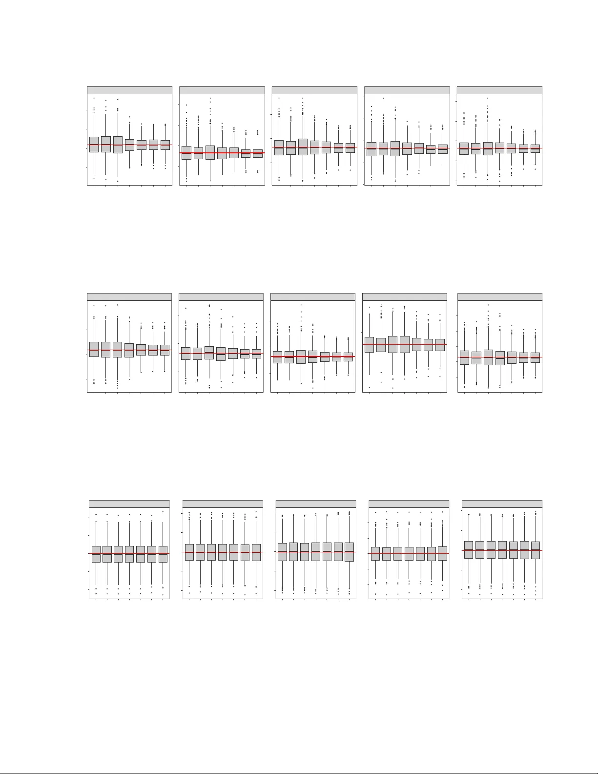
Generalized En trop y Calibration for Inference with P artially Observ ed Data: A Uniﬁed F ramew ork Mst Moush umi P ervin Departmen t of Statistics, Io w a State Univ ersit y , Io w a, USA and Hengfang W ang Sc ho ol of Mathematics and Statistics, F ujian Normal Univ ersit y , China and Jae Kw ang Kim Departmen t of Statistics, Io w a State Univ ersit y , Io w a, USA Abstract Missing data is an univ ersal problem in statistics. W e dev elop a uniﬁed frame- w ork for estimating parameters deﬁned b y general estimating equations under a missing-at-random (MAR) mec hanism, based on generalized entrop y calibration w eighting. W e construct w eights by minimizing a con vex entrop y sub ject to (i) bal- ancing constrain ts on a data-adaptiv e calibration function, estimated using ﬂexible mac hine-learning predictors with cross-ﬁtting, and (ii) a debiasing constraint in volv- ing the ﬁtted propensity score (PS) mo del. The resulting estimator is doubly robust, remaining consistent if either the outcome regression (OR) or the PS mo del is cor- rectly speciﬁed, and attains the semiparametric eﬃciency b ound when b oth models are correctly sp eciﬁed. Our form ulation encompasses classical in verse probabilit y w eighting (IPW) and augmented IPW (AIPW) as special cases and accommo dates a broad class of entrop y functions. W e illustrate the v ersatilit y of the approac h in three imp ortan t settings: semi-sup ervised learning with unlab eled outcomes, regres- sion analysis with missing cov ariates, and causal eﬀect estimation in observ ational studies. Extensive simulation studies and real-data applications demonstrate that the prop osed estimators achiev e greater eﬃciency and n umerical stabilit y than exist- ing metho ds. In particular, the prop osed estimator outperforms the classical AIPW estimator under the OR mo del missp eciﬁcation. Keywor ds: Calibration estimation, doubly robust, information pro jection, selection bias. 1 1 In tro duction Missing and incomplete data arise routinely in medical research, the so cial sciences, eco- nomics, and many other empirical disciplines. When the observed units are not repre- sen tativ e of the target population, na ¨ ıv e complete-case analysis can pro duce biased and ineﬃcien t inference. A cen tral goal of the missing-data literature is therefore to dev elop consisten t and eﬃcien t estimators under plausible assumptions ab out the missingness mec hanism (Little and Rubin, 2019; Kim and Shao, 2021). Man y mo dern data-analytic tasks can b e viewed through the lens of partially observed data. In semi-sup ervised learning, the c hallenge is to exploit a large p o ol of unlab eled co v ariates for eﬃciency while guarding against co v ariate-shift bias (Chap elle et al., 2010; Zhang et al., 2019). In causal inference, systematic co v ariate im balance betw een treatmen t groups m ust b e corrected through w eigh ting or matching (Hainm ueller, 2012; Li et al., 2018). In regression with missing cov ariates, complete-case analysis is generally biased under missing at random (MAR; Ibrahim et al., 2005; Han and W ang, 2013). All three settings share a common structure: a parameter deﬁned by an estimating equation that cannot be solved directly b ecause part of the data vector is unobserved. Tw o broad strategies exist. Outcome regression (OR) imputes the missing comp o- nen ts via a conditional exp ectation model. Prop ensit y-score (PS) w eighting constructs in v erse-probability w eights (IPW). Doubly robust (DR) methods suc h as augmen ted IPW (AIPW; Robins et al., 1994) combine b oth and yield consistent estimators if either mo del is correctly sp eciﬁed. How ever, as demonstrated by Kang et al. (2007), standard DR estimators can b e highly unstable with extreme weigh ts. T argeted minimum loss-based estimation (TMLE; v an der Laan and Rose, 2011) pro vides an alternativ e DR approach via a targeting step, but relies on a substitution estimator and does not directly pro duce calibration weigh ts for the observ ed units. In parallel, en trop y-based calibration metho ds c ho ose weigh ts by minimizing a conv ex div ergence sub ject to balancing constrain ts (Zu- bizarreta, 2015; Chan et al., 2016; Zhao, 2019; T an, 2020), achieving improv ed stability . These are closely related to cov ariate balancing metho ds in causal inference (F an et al., 2 2022; W ang and Zubizarreta, 2020; Chattopadhy ay et al., 2020; Hirsh b erg and W ager, 2021; Ben-Mic hael et al., 2021). Ho wev er, existing calibration form ulations do not di- rectly yield a general doubly robust framework for arbitrary estimating equations with partially observ ed data. In this pap er, we dev elop a uniﬁed framew ork for analyzing partially observed data under MAR by combi ning generalized entrop y calibration with doubly robust estimation and mo dern mac hine learning. The calibration w eights are obtained b y minimizing a gen- eralized en trop y sub ject to t w o sets of constrain ts: a balancing constrain t based on a calibration function that approximates the optimal augmen tation term, and a debiasing constrain t incorp orating a w orking PS mo del. T o ﬂexibly approximate the optimal cali- bration function, w e embed cross-ﬁtted mac hine-learning predictions in to the calibration step, follo wing the prediction-p ow ered (Angelop oulos et al., 2023) and double machine learning (Chernozh uko v et al., 2018) literatures. The presen t w ork builds on the generalized entrop y calibration framework of Kwon et al. (2025), which was dev elop ed for estimating ﬁnite p opulation totals under design- based inference with known auxiliary v ariables. W e extend their framew ork in three k ey directions. First, the target of inference is generalized from p opulation totals to solutions of estimating equations E { U ( θ ; Z ) } = 0 under arbitrary MAR structures, whic h introduces a θ -dep enden t calibration function requiring proﬁle optimization (Algorithm 1) with no coun terpart in the survey setting. Second, we establish double robustness and sho w that the prop osed estimator achiev es a strictly smaller asymptotic v ariance than AIPW under outcome mo del missp eciﬁcation (Corollary 3), results that ha ve no analog in the design- based framework where consistency follows from the known sampling mec hanism. This v ariance-reduction prop ert y distinguishes our approac h from b oth TMLE and the regu- larized calibrated estimation of T an (2020), neither of whic h pro vides a similar mec hanism under outcome-model missp eciﬁcation. Third, we develop a cross-ﬁtting pro cedure that in tegrates machine-learning predictions into the calibration constrain ts, and demonstrate the unifying scop e of the approach across causal inference, semi-sup ervised learning, and missing co v ariate problems. 3 The main con tributions are as follo ws. First, w e form ulate semi-sup ervised learning, re- gression with missing co v ariates, and causal inference within a single calibration-weigh ting framew ork for general estimating equations under MAR. Second, w e developed a doubly robust generalized entrop y calibration estimator that is doubly robust and lo cally eﬃcient. Third, we developed a prediction-p ow ered calibration. Cross-ﬁtted mac hine-learning pre- dictions enable ﬂexible nonparametric calibration while maintaining v alid large-sample theory . Sim ulations and real-data applications demonstrate substan tial eﬃciency gains and impro ved stabilit y , particularly under OR mo del missp eciﬁcation. The remainder of the pap er is organized as follo ws. Section 2 introduces the setup and reviews IPW and AIPW. Section 3 presen ts the proposed estimators. Section 4 establishes large-sample prop erties. Section 5 discusses computation. Section 6 illustrates applications to causal inference, semi-sup ervised learning, and missing cov ariates. Section 7 rep orts sim ulations, and Section 8 presen ts real-data applications. Some concluding remarks are made in Section 9. All the tec hnical pro ofs are relegated to the supplementary material (SM). 2 Preliminaries and Existing Metho ds Let Z = ( X ⊤ , Y ) ⊤ b e a ( p + 1)-dimensional random v ector where X ∈ R p denotes co- v ariates and Y is the outcome v ariable. Supp ose we observ e indep enden t and identically distributed copies Z 1 , . . . , Z N of Z . F or each unit i , decomp ose the full data vector as Z i =  O ⊤ i , M ⊤ i  ⊤ , (2.1) where O i is the alwa ys-observed subv ector and M i is the p otentially missing sub vector. This decomposition encompasses several familiar settings: 1. Missing outcomes: O i = X i , M i = Y i ; 2. Missing co v ariates: O i = Y i , M i = X i ; 3. P artially missing co v ariates: O i = ( X 1 i , Y i ) ⊤ , M i = X 2 i , where X i = ( X ⊤ 1 i , X ⊤ 2 i ) ⊤ . 4 Eac h setting is dev elop ed in detail in Section 6. Let δ i = 1 if M i is observ ed and δ i = 0 otherwise, and assume a missing-at-random (MAR) mec hanism (Rubin, 1976): δ i ⊥ M i | O i . Let θ ∈ R q denote the parameter of inter- est, deﬁned as the unique solution to the p opulation estimating equation E { U ( θ ; Z ) } = 0, where U ( θ ; Z ) is a q × 1 estimating function. Without missing data, θ can b e estimated b y solving ˆ U N ( θ ) ≡ N X i =1 U ( θ ; z i ) = 0 . (2.2) When M i is missing for some units, U ( θ ; z i ) is not fully computable and (2.2) cannot b e solv ed directly . Under MAR, a common strategy is to mo del the response mechanism via a propensity- score (PS) model, P ( δ i = 1 | O i ) = π ( O i ; ϕ ) , (2.3) where ϕ is a ﬁnite-dimensional parameter estimated by maxim um likelihoo d. The inv erse- probabilit y-w eighted (IPW) estimator of θ solves N X i =1 δ i π ( O i ; ˆ ϕ ) U ( θ ; z i ) = 0 . (2.4) Under correct speciﬁcation of (2.3), the IPW estimator is consistent for θ but can b e ineﬃcien t, as it discards partial information from units with δ i = 0, and numerically unstable when some π ( O i ; ˆ ϕ ) are near zero. T o impro v e eﬃciency , Robins et al. (1994) prop osed the augmen ted IPW (AIPW) estimator, whic h solves N X i =1 " δ i U ( θ ; z i ) π ( O i ; ˆ ϕ ) − δ i − π ( O i ; ˆ ϕ ) π ( O i ; ˆ ϕ ) b ( O i ) # = 0 , (2.5) where b ( O i ) is an arbitrary function of O i . The c hoice of b ( O i ) is of central importance. A particularly important target is b ∗ ( θ ; O i ) = E { U ( θ ; Z i ) | O i } , (2.6) 5 the conditional exp ectation of the estimating function given O i . If an OR mo del is sp eciﬁed for E { U ( θ ; Z i ) | O i } and correctly estimated, then using (2.6) in the AIPW estimator yields an estimator that is appro ximately un biased ev en when the PS mo del is missp eciﬁed. Consequen tly , the AIPW estimator enjo ys a doubly robust prop ert y if either the PS mo del or the OR mo del is correctly sp eciﬁed, and lo cally eﬃcien t if b oth are correct (Robins et al., 1994). Ho w ever, the AIPW estimator relies on an explicit augmentation term b ( O i ) and can b e sensitiv e to extreme inv erse-probability w eights, motiv ating the calibration-based ap- proac h dev elop ed in Section 3. 3 Prop osed Estimators W e propose an alternativ e to AIPW that constructs data-adaptive w eights ω i = ω ( O i ) through a generalized entrop y calibration pro cedure. Rather than using an explicit aug- men tation term, the method incorp orates auxiliary information implicitly via calibration constrain ts, preserving double robustness while improving numerical stabilit y . W e deﬁne the estimator ˆ θ ω as the solution to the w eighted estimating equation N X i =1 δ i ˆ ω i ( θ ) U ( θ ; z i ) = 0 , (3.1) where ˆ ω i ( θ ) = ˆ ω ( θ ; O i ) are calibration weigh ts that ma y dep end on θ , since the relev ant auxiliary information for estimating θ may itself dep end on θ . T o determine ˆ ω i ( θ ), w e employ the generalized en trop y calibration metho d of Kw on et al. (2025). Let G : ν → R b e a strictly con vex, diﬀerentiabl e function with deriv ative g = G ′ . The calibration weigh ts for the observ ed units ( δ i = 1) are obtained b y solving min ω 1 ,...,ω N N X i =1 δ i G ( ω i ) , (3.2) sub ject to the b alancing c onstr aint N X i =1 δ i ω i b ( O i ) = N X i =1 b ( O i ) , (3.3) 6 T able 1: Examples of generalized en tropies G ( ω ), the corresp onding calibration cov ariates ˆ g i = g ( ˆ π − 1 i ) and ˆ g − 1 i . En trop y G ( ω ) ˆ g i ˆ g − 1 i Domain Squared loss ω 2 / 2 ˆ π − 1 i ˆ π i ( −∞ , ∞ ) Empirical lik eliho o d − log ω − ˆ π i − 1 / ˆ π i (0 , ∞ ) Exp onen tial tilting ω log ω − ω log( ˆ π − 1 i ) 1 / log( ˆ π − 1 i ) (0 , ∞ ) Hellinger distance − √ ω − p ˆ π i / 2 − p 2 / ˆ π i (0 , ∞ ) and the debiasing c onstr aint N X i =1 δ i ω i g ( ˆ π − 1 i ) = N X i =1 g ( ˆ π − 1 i ) , (3.4) where ˆ π i = π ( O i ; ˆ ϕ ) is the ﬁtted PS mo del. The balancing constraint (3.3) forces the w eigh ted complete cases to repro duce the sample moments of the calibration function b ( O ). The debiasing constraint (3.4) uses the transformed inv erse prop ensit y scores g ( ˆ π − 1 i ) to align the calibration w eights with IPW weigh ts when the PS mo del is correctly sp eciﬁed. The calibration link function g ( ˆ π − 1 i ) arises because g = G ′ and the optimal w eights from (3.2) tak e the form ω ∗ i = g − 1 ( λ ⊤ s i ) (see Section 3.1). When the PS mo del is correct and calibration is based solely on the debiasing constrain t, the solution satisﬁes ω ∗ i = g − 1 ( g ( π − 1 i )) = π − 1 i , recov ering the standard IPW w eights exactly . Th us, the choice of g ( ˆ π − 1 i ) as the debiasing co v ariate is not ad ho c but is dictated b y the en tropy function G to ensure that the calibration w eights reduce to IPW under the correct PS mo del. In tuitiv ely , if w e use b ∗ ( O ) = E  U ( θ ; Z ) | O  in the balancing constrain t and the OR mo del used to construct b ∗ ( O ) is correct, balancing remov es the leading bias term ev en when the PS mo del is wrong; con versely , if the PS mo del is correct, the debiasing constrain t ensures consistency ev en when the OR mo del is wrong. These properties are formalized in Section 4. Diﬀeren t c hoices of the en tropy function G pro duce diﬀeren t w eighting sc hemes; sev eral examples are summarized in T able 1. 7 3.1 Dual form ulation The constrained optimization (3.2)–(3.4) is solved eﬃcien tly through its dual. In tro duce Lagrange multipliers λ 1 ∈ R q and λ 2 ∈ R for constraints (3.3)–(3.4), and write b i = b ( O i ), ˆ g i = g ( ˆ π − 1 i ), and s i = ( b ⊤ i , ˆ g i ) ⊤ . The Lagrangian is Q ( ω , λ ) = − N X i =1 δ i G ( ω i ) + λ ⊤ 1   N X i =1 δ i ω i b i − N X i =1 b i   + λ 2   N X i =1 δ i ω i ˆ g i − N X i =1 ˆ g i   , (3.5) where λ =  λ ⊤ 1 , λ 2  ⊤ . Maximizing Q ( ω , λ ) with respect to ω i yields the closed-form opti- mal w eights ω ∗ i ( λ ) = g − 1 ( λ ⊤ 1 b i + λ 2 ˆ g i ) = g − 1 ( λ ⊤ s i ) , (3.6) where λ = ( λ ⊤ 1 , λ 2 ) ⊤ and g − 1 is strictly increasing b ecause G is strictly con vex. The function g ( · ) is called the calibration link function and is closely related to the canonical link function in the generalized linear mo dels. The calibration link op erates on the weigh t parameter ω i rather than a conditional mean µ i , but the algebraic structure is identical. Substituting (3.6) bac k to (3.5) giv es the dual ob jective ρ G ( λ ) = 1 N N X i =1 δ i F ( λ ⊤ s i ) − 1 N N X i =1 λ ⊤ s i , (3.7) where F ( ν ) = − G { g − 1 ( ν ) } + g − 1 ( ν ) ν is the conv ex conjugate of G . The optimal dual solution ˆ λ = arg min λ ρ G ( λ ) determines the ﬁnal weigh ts ˆ ω i = ω ∗ i ( ˆ λ ). Diﬀeren tiating (3.7) conﬁrms that ˆ λ satisﬁes the calibration equations (3.3)–(3.4): ∂ ∂ λ ρ G ( λ ) = 1 N    N X i =1 δ i ω ∗ i ( λ ) s i − N X i =1 s i    . F or this reason, w e refer to ρ G ( λ ) as the calibration generating function induced by the en trop y G . The dual representation reduces the problem to optimizing ov er λ ∈ R q +1 , regardless of the sample size N . 8 4 Large-Sample Prop erties W e establish the asymptotic properties of the prop osed estimator ˆ θ ω deﬁned in (3.1). Throughout, the estimator solves ˆ U ω ( θ ) ≡ N X i =1 δ i ω ∗ i ( ˆ λ, ˆ φ ) U ( θ ; z i ) = 0 , where ω ∗ i ( λ, φ ) = g − 1  λ ⊤ 1 b i + λ 2 g i ( φ )  , b i = b ( O i ), and g i ( φ ) = g { π − 1 ( O i ; φ ) } . The pa- rameters ˆ φ and ˆ λ are obtained jointly from ∇ ℓ ( φ ) ≡ 1 N N X i =1  δ i π i − 1  h i ( φ ) = 0 , (4.1) ∇ ˆ ρ G ( λ ) ≡ 1 N N X i =1 ( δ i ω ∗ i ( λ, ˆ φ )    b i g i ( ˆ φ )    −    b i g i ( ˆ φ )    ) = 0 , (4.2) where π i = π ( O i ; φ ) and h i ( φ ) = { 1 − π i ( φ ) } − 1 ∂ π i ( φ ) /∂ φ . The regularit y conditions are collected in the Supplemen tary Material (SM), Section A. Assumptions 1–2 ensure the consistency of ˆ φ and ˆ λ , established in Lemma S.1 of the SM. Assumptions 3–4 imp ose smo othness and non-degeneracy of the limiting dual and prop ensit y-score ob jectiv es; in particular, non-singularit y of hessian E {∇ 2 ρ G ( λ ∗ ) } , where λ ∗ = arg min λ ρ G ( λ ) and ρ G ( λ ) is deﬁned in (3.7), requires that the calibration co v ariates s i = ( b ⊤ i , g i ) ⊤ are not collinear among the resp ondents, which is the natural iden tiﬁabil- it y condition for entrop y calibration. Assumptions 5–7 are standard conditions for joint M-estimation of the system (4.1)–(4.2); they hold whenev er the three sub-problems are individually w ell-p osed and their in teraction is smo oth. 4.1 Linearization The following theorem pro vides a ﬁrst-order linear expansion of ˆ U ω ( θ ) that underlies all subsequen t asymptotic results. 9 Theorem 4.1 (Linearization) . Under Assumptions 1–4, ˆ U ω ( θ ) = ˜ U ω ( λ ∗ , ˆ φ ) + o p ( N − 1 / 2 ) , wher e ˜ U ω ( λ ∗ , ˆ φ ) = 1 N N X i =1 h γ ∗ s i ( ˆ φ ) + δ i ω ∗ i ( λ ∗ , ˆ φ )  U ( θ ; z i ) − γ ∗ s i ( ˆ φ )  i , s i ( ˆ φ ) =  b ⊤ i , g ( π − 1 ( O i ; ˆ φ ))  ⊤ , and γ ∗ ∈ R q × ( q +1) is the pr ob ability limit of ˆ γ satisfying N X i =1 δ i f ′  λ ∗⊤ s i ( ˆ φ )   U ( θ ; z i ) − γ s i ( ˆ φ )  s ⊤ i ( ˆ φ ) = 0 , with f ′ = ( g − 1 ) ′ . This exp ansion holds without assuming c orr e ctness of either the PS or the OR mo del. The linearization decomp oses ˆ U ω ( θ ) into a full-sample pro jection term γ ∗ s i ( ˆ φ ) and a resp onden t-only residual term. The co eﬃcient γ ∗ is the p opulation weigh ted-least-squares pro jection of U ( θ ; Z ) onto the calibration co v ariates S ( O ; φ ∗ ) where φ ∗ = arg max φ E { ℓ ( φ ) } , so the decomposition is in terpretable as a calibration-based augmentation. 4.2 Consistency under the correct PS mo del W e ﬁrst show that the calibration w eigh ts reduce to IPW weigh ts when the PS mo del is correct, and deriv e the resulting asymptotic distribution. Lemma 4.1. If the PS model is correctly sp eciﬁed, i.e., P ( δ = 1 | O ) = π ( O ; φ 0 ), then φ ∗ = φ 0 and λ ∗ 1 → 0, λ ∗ 2 → 1, so that ω ∗ i ( λ ∗ , φ 0 ) = 1 /π ( O i ; φ 0 ). Corollary 1 (Asymptotic normality under correct PS mo del) . Under Assumptions 1–7 and a c orr e ctly sp e ciﬁe d PS mo del, √ N ( ˆ θ ω − θ 0 ) d − → N  0 , τ − 1 1 V 1 ( τ − 1 1 ) ⊤  , wher e τ 1 = E  ∂ U ( θ 0 ; Z ) /∂ θ ⊤  and V 1 = V ar  U ( θ 0 ; Z )  + E "  1 π ( O ; φ 0 ) − 1   U ( θ 0 ; Z ) − γ ∗ S ( O ; φ 0 ) − κ ∗ h ( O ; φ 0 )  ⊗ 2 # , 10 with S ( O ; φ 0 ) =  b ⊤ ( O ) , g ( π − 1 ( O ; φ 0 ))  ⊤ and B ⊗ = B B ⊤ . Her e κ ∗ ∈ R q × r is the pr ob a- bility limit of ˆ κ deﬁne d by 1 N N X i =1 ∂ ∂ φ  γ ∗ s i ( φ ) + δ i ω ∗ i ( λ ∗ , φ )  U ( θ ; z i ) − γ ∗ s i ( φ )  +  1 − δ i π ( O i ; φ )  κ h i ( φ )  = 0 . (4.3) The term κ ∗ h ( O ; φ 0 ) c aptur es the eﬀe ct of estimating φ on the asymptotic varianc e; it vanishes when the OR mo del is also c orr e ctly sp e ciﬁe d. 4.3 Consistency under the correct OR mo del Lemma 4.2. If the OR mo del is correctly sp eciﬁed, i.e., E { U ( θ 0 ; Z ) | O } ∈ span { b ( O ) } , and b ∗ ( O ) = E { U ( θ ; Z ) | O } is used in (3.3), then κ ∗ = 0. Corollary 2 (Asymptotic normalit y under correct OR model) . Under Assumptions 1–7, if b ∗ ( O ) = E { U ( θ ; Z ) | O } satisﬁes E { U ( θ 0 ; Z ) | O } ∈ span { b ( O ) } , then √ N ( ˆ θ ω − θ 0 ) d − → N  0 , τ − 1 1 ¯ V 1 ( τ − 1 1 ) ⊤  , wher e ¯ V 1 = V ar  E [ U ( θ 0 ; Z ) | O ]  + E h δ  ω ∗ ( O ; λ ∗ , φ ∗ )  2 V ar { U ( θ 0 ; Z ) | O } i . Henc e ˆ θ ω r emains √ N -c onsistent and asymptotic al ly normal even when the PS mo del is missp e ciﬁe d. 4.4 Double robustness, v ariance dominance, and lo cal eﬃciency Corollaries 1 and 2 together establish that ˆ θ ω is doubly r obust : it is consisten t for θ 0 if either the PS or the OR mo del is correctly sp eciﬁed. W e no w show that, under a correct PS model, the proposed estimator is nev er less eﬃcien t than the classical AIPW estimator and is strictly more eﬃcient whenev er the OR mo del is missp eciﬁed and the debiasing co v ariate carries additional information. 11 Corollary 3 (V ariance dominance o ver AIPW) . Under the c onditions of Cor ol lary 1, let V 1 denote the varianc e c omp onent of the pr op ose d estimator ˆ θ ω and let V 3 = V ar  U ( θ 0 ; Z )  + E "  1 π ( O ; φ 0 ) − 1   U ( θ 0 ; Z ) − b ( O )  ⊗ 2 # b e the c orr esp onding varianc e c omp onent of the classic al AIPW estimator. Then V 1 ≤ V 3 , (4.4) with e quality if and only if g  π − 1 ( O ; φ 0 )  and h ( O ; φ 0 ) lie in span { b ( O ) } almost sur ely. The v ariance reduction is most pronounced when the OR mo del is substan tially mis- sp eciﬁed, so that b ( O ) is a p o or approximation to E { U ( θ 0 ; Z ) | O } , but the PS mo del pro vides useful information ab out the missingness mechanism through the debiasing co- v ariate g ( π − 1 ( O ; φ 0 )) and the score function h ( O ; φ 0 ). In such settings, the en tropy cali- bration framew ork eﬀectiv ely enric hes the augmen tation space beyond what AIPW uses, yielding strictly smaller asymptotic v ariance without requiring any additional mo deling eﬀort. Remark 1. When b oth mo dels ar e c orr e ctly sp e ciﬁe d and b ∗ ( O ) = E { U ( θ ; Z ) | O } is use d in c alibr ation, b oth V 1 and V 3 r e duc e to V ∗ 1 = V ar  U ( θ 0 ; Z )  + E "  1 π ( O ; φ 0 ) − 1  V ar { U ( θ 0 ; Z ) | O } # , which c oincides with the semip ar ametric eﬃciency lower b ound of R obins et al. (1994). Thus, the pr op ose d estimator is also lo c al ly eﬃcient. 5 Computational Details This section describ es the n umerical implementation of ˆ θ ω . The dual form ulation in Section 3.1 reduces the calibration step to an unconstrained con v ex minimization ov er λ ∈ R q +1 . W e now address t wo additional computational issues: (i) solving the nested op- timization when the calibration function b ( O i ) dep ends on θ , and (ii) constructing b ( O i ) via cross-ﬁtted mac hine-learning predictions. 12 Algorithm 1 Tw o-Lo op Proﬁle Optimization for ˆ θ ω Require: Initial v alue θ (0) ; tolerances ϵ > 0, δ > 0 1: k ← 0 2: rep eat 3: Inner lo op: Compute ˆ λ ( θ ( k ) ) = arg min λ ρ G ( λ, θ ( k ) ) 4: Outer lo op: Up date θ ( k +1) ← θ ( k ) − [ ∇ 2 θ L ( θ ( k ) )] − 1 ∇ θ L ( θ ( k ) ) 5: k ← k + 1 6: un til ∥ θ ( k ) − θ ( k − 1) ∥ ≤ ϵ or ∥∇ θ L ( θ ( k − 1) ) ∥ ≤ δ 7: return ˆ θ ω ← θ ( k ) 5.1 Proﬁle optimization The optimal calibration function is b ∗ ( θ ; O i ) = E { U ( θ ; Z i ) | O i } , whic h dep ends on the unkno wn parameter θ . Under this c hoice, the dual ob jective b ecomes ρ G ( λ, θ ), with s i ( θ ) = ( b ∗⊤ ( θ ; O i ) , g i ( ˆ ϕ )) ⊤ , and the estimator solves the saddle-p oin t problem ˆ θ ω = arg max θ min λ ρ G ( λ, θ ) . (5.1) Equiv alen tly , deﬁning the proﬁle ob jective L ( θ ) = ρ G ( ˆ λ ( θ ) , θ ) where ˆ λ ( θ ) = arg min λ ρ G ( λ, θ ), w e ha v e ˆ θ ω = arg max θ L ( θ ). W e solv e (5.1) using a tw o-lo op pro cedure. F or a ﬁxed θ , the inner lo op minimizes ρ G ( λ, θ ) o ver λ using Newton’s metho d. The outer lo op up dates θ via a Newton or BFGS step based on the gradien t of L ( θ ). By the en velope theorem (Danskin, 2012), ∇ θ L ( θ ) = ∇ θ ρ G ( ˆ λ ( θ ) , θ ), since ∇ λ ρ G = 0 at the inner optimum. The procedure is summarized in Algorithm 1. 5.2 Calibration via cross-ﬁtting In practice, the conditional exp ectation b ∗ ( θ ; O i ) = E { U ( θ ; Z i ) | O i } is unkno wn and m ust b e estimated. F ollowing the idea of Angelop oulos et al. (2023), we appro ximate it b y plugging in a prediction ˆ M i of the missing component M i : b ∗ ( θ ; O i ) ≈ U ( θ ; O i , ˆ M i ), 13 where ˆ M i is obtained from a ﬂexible mac hine-learning model ﬁtted to the observ ed data. T o a void the o verﬁtting bias that arises from using the same data to train the prediction rule and to estimate θ (Chernozhuk o v et al., 2018), we adopt K -fold cross-ﬁtting. Let I = { 1 , . . . , N } and S = { i ∈ I : δ i = 1 } . W e randomly partition I into K disjoint folds {I ( k ) } K k =1 . F or eac h fold k , we ﬁt a prediction mo del ˆ m ( − k ) ( · ) using training data S ( − k ) = S \ ( S ∩ I ( k ) ) and compute out-of-fold predictions ˆ M ( − k ) i = ˆ m ( − k ) ( O i ) for i ∈ I ( k ) . Using these cross-ﬁtted predictions, we solve the calibration problem: min ω 1 ,...,ω N N X i =1 δ i G ( ω i ) , (5.2) sub ject to K X k =1 X i ∈I ( k ) δ i ω i U  θ ; O i , ˆ M ( − k ) i  = K X k =1 X i ∈I ( k ) U  θ ; O i , ˆ M ( − k ) i  , (5.3) N X i =1 δ i ω i g ( ˆ π − 1 i ) = N X i =1 g ( ˆ π − 1 i ) . (5.4) The t wo-loop pro cedure in Algorithm 1 is then applied to obtain ˆ θ ω . Note that the prediction mo del ˆ m ( − k ) is trained only on the complete cases in S ( − k ) , but the out-of-fold predictions ˆ M ( − k ) i are computed for al l units i ∈ I ( k ) , including those with δ i = 0. This is essential: the balancing constrain t (5.3) in volv es the full sample, so calibration function v alues are needed for every unit regardless of whether M i is observ ed. Remark 2. The asymptotic r esults in Se ction 4 r e quir e the cr oss-ﬁtte d pr e dictor ˆ m ( − k ) to satisfy a me an-squar e d-err or c ondition of the form E ∥ ˆ M ( − k ) i − E ( M i | O i ) ∥ 2 = o (1) , i.e., the pr e diction err or must vanish in pr ob ability. This c ondition is mild and is satisﬁe d by a br o ad r ange of mo dern machine-le arning metho ds, including r andom for ests, gr adient b o osting, neur al networks, and p enalize d r e gr ession, pr ovide d the sample size gr ows and standar d r e gularity c onditions hold. No sp e ciﬁc c onver genc e r ate (e.g., N − 1 / 4 ) is r e quir e d for the cr oss-ﬁtte d pr e dictions, b e c ause the debiasing c onstr aint ensur es that the estimator r emains c onsistent even when the pr e diction mo del c onver ges slow ly, as long as the PS mo del is c orr e ctly sp e ciﬁe d. When neither mo del is c orr e ctly sp e ciﬁe d, faster c onver genc e of the pr e dictor gener al ly impr oves ﬁnite-sample p erformanc e, though c onsistency is no longer guar ante e d. Se e Se ction C of SM for mor e details. 14 6 Illustrativ e Examples W e no w describe ho w the prop osed framew ork applies to three important settings. In eac h case, we sp ecify the decomp osition ( O i , M i ), the estimating function U ( θ ; Z i ), and the calibration function b ( θ ; O i ); the calibration w eights and estimator are then obtained b y applying the general pro cedure in Sections 3 – 5. 6.1 Causal inference Let T i ∈ { 0 , 1 } b e a binary treatmen t indicator, Y i (1) and Y i (0) are the p oten tial out- comes, and X i ∈ R p the observ ed cov ariates. Under SUTV A, unconfoundedness, and p ositivit y (Rubin, 1974; Rosenbaum and Rubin, 1983; Imbens and Rubin, 2015), the ob- serv ed outcome is Y i = T i Y i (1) + (1 − T i ) Y i (0) and the a verage treatment eﬀect (A TE) is θ = θ 1 − θ 0 = E { Y (1) } − E { Y (0) } , where θ t solv es E { U t ( θ t ; X , Y ( t )) } = 0 with U t ( θ t ; X , Y ( t )) = Y ( t ) − θ t for t ∈ { 0 , 1 } . W e estimate θ 1 and θ 0 separately . F or eac h t ∈ { 0 , 1 } , deﬁne δ i = 1 ( T i = t ), O i = X i , M i = Y i ( t ), and π ( X i ; ϕ ) = P ( T i = t | X i ). The calibration function is b ( θ t ; X i ) = U t ( θ t ; X i , ˆ Y i ( t )) = ˆ Y i ( t ) − θ t , where ˆ Y i ( t ) are cross-ﬁtted predictions. F or the treated group ( t = 1), the calibration w eights { ω 1 i } N i =1 are obtained b y solving min ω 11 ,...,ω 1 N N X i =1 T i G ( ω 1 i ) , (6.1) sub ject to N X i =1 T i ω 1 i = N , (6.2) N X i =1 T i ω 1 i  ˆ Y i (1) − θ 1  = N X i =1  ˆ Y i (1) − θ 1  , (6.3) N X i =1 T i ω 1 i g ( ˆ π − 1 i ) = N X i =1 g ( ˆ π − 1 i ) , (6.4) 15 where ˆ π i = P ( T i = 1 | X i ; ˆ ϕ ) is the estimated prop ensit y score. An analogous calibration problem is solved within the control group ( t = 0) to obtain w eigh ts { ω 0 i } N i =1 and the estimate ˆ θ 0 . Because the balancing constrain t (6.3) dep ends on θ t , we apply the t wo-loop proﬁle optimization (Algorithm 1) within each treatmen t group to jointly estimate θ t and the corresponding weigh ts, and form ˆ θ = ˆ θ 1 − ˆ θ 0 . 6.2 Semi-sup ervised learning In man y applied settings, the outcome v ariable is exp ensiv e or diﬃcult to obtain while co v ariates are readily av ailable. F or example, in electronic health records research, clini- cal diagnoses require exp ert review but demographic and lab oratory cov ariates are rou- tinely recorded (Gronsb ell and Cai, 2018; Chakrab ortt y and Cai, 2018). Semi-sup ervised metho ds aim to exploit the large p o ol of unlab eled co v ariates to improv e eﬃciency ov er sup ervised analysis that uses only the labeled sample. F ormally , a labeled dataset L = { ( x i , y i ); i = 1 , . . . , n } with fully observed outcomes is supplemented by an unlabeled dataset U = { x i ; i = n + 1 , . . . , n + N } . Here Z i = ( X i , Y i ), O i = X i , M i = Y i , and δ i = 1 if Y i is observed. The target parameter θ solv es E { U ( θ ; X , Y ) } = 0, and the calibration function is b ( θ ; X i ) = U ( θ ; X i , ˆ Y i ), where ˆ Y i are cross-ﬁtted predictions of Y i based on X i . The selection mec hanism may b e either MAR, with P ( δ i = 1 | X i ) = π ( X i ; ϕ ) estimated b y logistic regression, or MCAR, with P ( δ i = 1) = n/ ( n + N ). In b oth cases, the calibration w eigh ts are obtained from (5.2)–(5.4) and the estimator from Algorithm 1. Concretely , the proposed estimator of θ solves the weigh ted estimating equation 1 n + N n + N X i =1 δ i ω i U ( θ ; x i , y i ) = 0 , (6.5) where the w eigh ts ω i in tegrate lab eled and unlab eled data through the balancing con- strain t, ensuring that the weigh ted labeled sample repro duces the co v ariate moments of the full sample. This yields a doubly robust semi-sup ervised estimator that remains ef- ﬁcien t ev en under OR mo del missp eciﬁcation: when the prediction mo del for Y i is p o or, 16 the debiasing constraint based on π ( X i ; ˆ ϕ ) still corrects for the distributional diﬀerence b et w een lab eled and unlab eled samples. 6.3 Missing co v ariates in regression Supp ose ( Y i , X i ) with X i = ( X 1 i , X 2 i ) are related b y a regression mo del Y i = µ ( X 1 i , X 2 i ; β )+ ϵ i with E ( ϵ i | X i ) = 0, and X 2 i is sub ject to missingness. Here O i = ( X 1 i , Y i ), M i = X 2 i , and δ i = 1 ( X 2 i observ ed). Under MAR, δ i ⊥ X 2 i | ( X 1 i , Y i ) , so that the probability of observing X 2 i ma y dep end on b oth the fully observ ed cov ariates X 1 i and the resp onse Y i , but not on the missing co v ariate X 2 i itself. This conditioning on Y i distinguishes the missing-cov ariate setting from the missing-outcome case: the prop ensit y score model is P ( δ i = 1 | X 1 i , Y i ) = π ( X 1 i , Y i ; ϕ ) , whic h can be estimated b y maxim um lik eliho o d, e.g., ˆ ϕ = arg max ϕ N X i =1  δ i log { π ( X 1 i , Y i ; ϕ ) } + (1 − δ i ) log { 1 − π ( X 1 i , Y i ; ϕ ) }  . The estimating function is U ( β ; X 1 i , X 2 i , Y i ) = { Y i − µ ( X 1 i , X 2 i ; β ) } ∂ ∂ β µ ( X 1 i , X 2 i ; β ) , and the calibration function is b ( β ; X 1 i , Y i ) = U ( β ; X 1 i , ˆ X 2 i , Y i ), where ˆ X 2 i are cross-ﬁtted predictions of X 2 i based on ( X 1 i , Y i ). The calibration w eights and estimator of β are obtained b y applying (5.2)–(5.4) and Algorithm 1. 7 Sim ulation Study W e ev aluate the prop osed Hellinger distance (HD) and exp onen tial tilting (ET) entrop y calibration estimators across the three application settings. All simulations use K = 4 folds for cross-ﬁtting unless otherwise noted. 17 7.1 Causal inference Design. W e consider a 2 × 2 factorial design with t w o outcome regression mo dels (OR1, OR2) and tw o prop ensit y score mo dels (PS1, PS2), using M = 500 Mon te Carlo replicates with sample size N = 1 , 000. Cov ariates are generated as x i = ( x i 1 , x i 2 , x i 3 , x i 4 ) ⊤ ∼ N (0 4 , I 4 ), and potential outcomes as y i ( t ) = m t ( x i ) + ε it , ε it ∼ N (0 , 1), t ∈ { 0 , 1 } . • OR1 (linear): m 1 ( x ) = 1 + 1 ⊤ x , m 0 ( x ) = 1 ⊤ x , 1 = (1 , 1 , 1 , 1) ⊤ ; true A TE = 1. • OR2 (nonlinear): Let h ( x ) = ( x − 1) 3 − x 2 + x/ { 1 + exp(clip( x )) } + 10 with clip( x ) = max { min( x, 3) , − 3 } applied component wise. Set m 1 ( x ) = 10 + 1 ⊤ x + 1 2 1 ⊤ h ( x ), m 0 ( x ) = 1 ⊤ x + 1 2 1 ⊤ h ( x ); true A TE = 10. • PS1 (logistic linear): π ( x ) = expit( − 0 . 25 + x 1 + 0 . 5 x 2 − 0 . 5 x 3 − 0 . 1 x 4 ). • PS2 (logistic nonlinear): π ( x ) = expit( x 1 − 0 . 5 x 1 x 2 − x 2 3 + 0 . 5 x 3 4 ). The treatmen t indicator is T i ∼ Bernoulli { π ( x i ) } and the observ ed outcome is Y i = T i Y i (1) + (1 − T i ) Y i (0). W e compare HD and ET with seven existing metho ds: in v erse probabilit y w eighting (IPW; Horvitz and Thompson, 1952), entrop y balancing (EBPS; Hainm ueller, 2012), optimal co v ariate balancing (oCBPS; F an et al., 2022), cov ariate bal- ancing propensity score (CBPS; Imai and Ratk o vic, 2014), empirical balancing calibration w eigh ting (EBCW; Chan et al., 2016), and AIPW with either a linear mo del or GAM for the outcome regression, denoted AIPW (LM) and AIPW (GAM). 18 0.8 1.0 1.2 1.4 IPW EBPS oCBPS CBPS EBCW AIPW (LM) AIPW (GAM) HD ET P oint estimate (a) OR1PS1 0.8 1.0 1.2 1.4 IPW EBPS oCBPS CBPS EBCW AIPW (LM) AIPW (GAM) HD ET P oint estimate (b) OR1PS2 8 10 12 14 IPW EBPS oCBPS CBPS EBCW AIPW (LM) AIPW (GAM) HD ET P oint estimate (c) OR2PS1 4 6 8 10 12 IPW EBPS oCBPS CBPS EBCW AIPW (LM) AIPW (GAM) HD ET P oint estimate (d) OR2PS2 Figure 1: Estimation of Average T reatment Eﬀects (A TE) under four scenarios: under OR1(2), the outcome regression (OR) mo del is correctly sp eciﬁed (misspeciﬁed); under PS1(2), the prop ensit y score mo del is correctly sp eciﬁed (missp eciﬁed). The horizontal red line represen ts the true A TE. Results. Figure 1 summarizes the Monte Carlo distributions across four speciﬁcation regimes. Under OR1PS1 (b oth mo dels correct), all metho ds sho w negligible bias and similar v ariability , consistent with the local eﬃciency result in Remark 1: when b oth mo dels are correctly sp eciﬁed, the prop osed estimator matches AIPW. 19 Under OR1PS2 (PS missp eciﬁed, OR correct), IPW and oCBPS exhibit substantial bias because they rely exclusively on the PS mo del, whereas HD, ET, and the remaining calibration-based and augmented estimators maintain low bias, conﬁrming the OR-based consistency path wa y in Corollary 2. The most informativ e comparison is OR2PS1 (OR misspeciﬁed, PS correct), whic h isolates the v ariance-reduction mec hanism identiﬁed in Corollary 3. Here, HD and ET displa y noticeably smaller in terquartile ranges than all competitors, including b oth AIPW v arian ts. Among the AIPW estimators, AIPW (GAM) sho ws a clear eﬃciency gain ov er AIPW (LM), as the more ﬂexible outcome mo del partially comp ensates for missp eciﬁ- cation; nev ertheless, b oth AIPW v ersions remain less eﬃcient than HD and ET. The w eigh ting-only metho ds (IPW, EBPS, oCBPS, CBPS, EBCW) show substan tially wider b o xplots, reﬂecting their lack of outcome-mo del augmen tation. Under joint missp eciﬁcation (OR2PS2), all metho ds are potentially inconsistent. Nev- ertheless, HD and ET remain the most robust, exhibiting the smallest bias and most concen trated sampling distributions, whic h suggests that the entrop y calibration frame- w ork degrades gracefully when neither mo del is fully correct. This is somewhat related to the global robustness of the HD discussed b y Antoine and Dov onon (2021). 7.2 Semi-sup ervised learning Design. The target is the regression coeﬃcient β in y i = x ⊤ i β + ϵ i . Cov ariates are x i ∼ N (0 p , I p ) with p = 4, total sample size n + N = 2 , 000, and M = 1 , 000 replications. The outcome is generated under t wo sp eciﬁcations: • OR1 (linear): y i = α 0 + α ⊤ 1 x i + ϵ i ; • OR2 (nonlinear): y i = α 0 + α ⊤ 1 x i + α ⊤ 2 { x 3 i − x 2 i + exp( x i ) } + ϵ i , where ( α 0 , α ⊤ 1 , α ⊤ 2 ) ⊤ = (1 , 1 ⊤ , 1 ⊤ ) ⊤ and ϵ i ∼ N (0 , 1). The true v alue of the target parame- ter β is computed by generating data of size 10 7 . Note that under OR2 the data-generating mo del is nonlinear, so the linear w orking mo del y i = x ⊤ i β + ϵ i is missp eciﬁed; nev erthe- less, β remains a w ell-deﬁned pro jection parameter that our metho d targets. Two selection 20 mec hanisms are considered: MAR , with logit( p i ) = − 1 − x 1 i − 0 . 5 x 2 i + 0 . 5 x 3 i + 0 . 1 x 4 i ; and MCAR , with p i = n/ ( n + N ). W e compare HD and ET with the sup ervised estima- tor (Sup) and four semi-sup ervised metho ds: the pro jection-based estimator (PSSE; Song et al., 2024), densit y-ratio estimation (DRESS; Kaw akita and Kanamori, 2013), eﬃcien t adaptiv e estimation (EASE; Chakrab ortt y and Cai, 2018), and the partial-information estimator (PI; Azriel et al., 2022). Results. Under OR mo del missp eciﬁcation (OR2) with MAR (Figure 2), HD and ET achiev e the highest eﬃciency among all metho ds for all ﬁv e regression co eﬃcien ts β 0 , . . . , β 4 . The impro vemen t is most visible for β 0 : the in terquartile range of HD and ET is roughly half that of the supervised estimator, and noticeably smaller than those of PI, EASE, DRESS, and PSSE. The existing semi-sup ervised metho ds (PI, EASE, DRESS, PSSE) pro vide only mo dest gains o ver the sup ervised estimator under OR misspeciﬁ- cation, b ecause their eﬃciency improv emen ts rely on the outcome mo del b eing appro xi- mately correct. In con trast, our prop osed estimators beneﬁt from the debiasing constrain t, whic h comp ensates for outcome-mo del missp eciﬁcation through the prop ensit y-score in- formation. Under OR2 with MCAR (Figure 3), the same pattern holds: HD and ET dominate in eﬃciency . The MCAR mec hanism simpliﬁes the selection mo del, so the debiasing con- strain t is particularly eﬀectiv e, and the eﬃciency gains of HD and ET o v er comp etitors are ev en more pronounced. Under a correctly sp eciﬁed OR mo del (OR1) with MCAR (Figure 4), all semi-sup ervised estimators—including HD, ET, PI, EASE, DRESS, and PSSE—are consisten t and nearly as eﬃcien t as the sup ervised estimator, conﬁrming that the prop osed metho d do es not sacriﬁce eﬃciency when the outcome mo del is correct. This is consisten t with the lo cal eﬃciency result (Remark 1): when b oth models are correctly sp eciﬁed, the calibration w eigh ts are close to unit y and the estimator b eha ves lik e the full-sample sup ervised esti- mator. 21 β 0 β 1 β 2 β 3 β 4 Sup PI EASE DRESS PSSE ET HD Sup PI EASE DRESS PSSE ET HD Sup PI EASE DRESS PSSE ET HD Sup PI EASE DRESS PSSE ET HD Sup PI EASE DRESS PSSE ET HD 4 5 6 7 8 4 5 6 7 8 5 6 7 5 6 7 8 3.0 3.5 4.0 4.5 Method P oint estimate Figure 2: Boxplots of the estimated linear regression co eﬃcien ts β under OR2 (OR mo del missp eciﬁcation) with MAR missingness. β 0 β 1 β 2 β 3 β 4 Sup PI EASE DRESS PSSE ET HD Sup PI EASE DRESS PSSE ET HD Sup PI EASE DRESS PSSE ET HD Sup PI EASE DRESS PSSE ET HD Sup PI EASE DRESS PSSE ET HD 5.0 5.5 6.0 6.5 7.0 5 6 5 6 7 5 6 7 3.0 3.5 4.0 4.5 Method P oint estimate Figure 3: Boxplots of the estimated linear regression co eﬃcien ts β under OR2 (OR mo del missp eciﬁcation) with MCAR missingness. β 0 β 1 β 2 β 3 β 4 Sup PI EASE DRESS PSSE ET HD Sup PI EASE DRESS PSSE ET HD Sup PI EASE DRESS PSSE ET HD Sup PI EASE DRESS PSSE ET HD Sup PI EASE DRESS PSSE ET HD 0.90 0.95 1.00 1.05 1.10 0.90 0.95 1.00 1.05 1.10 0.90 0.95 1.00 1.05 1.10 0.90 0.95 1.00 1.05 1.10 0.90 0.95 1.00 1.05 1.10 Method P oint estimate Figure 4: Estimation of the linear regression co eﬃcien ts β under OR1 (when the OR mo del is correctly sp eciﬁed) and MCAR missingness mec hanism. 22 7.3 Missing co v ariates in regression Design. W e estimate β = ( β 0 , β 1 , β 2 ) in the linear mo del y i = β 0 + β 1 x 1 i + β 2 x 2 i + ϵ i , where x 1 i ∼ N (0 , 1), x 2 i ∼ Bernoulli(0 . 5), ϵ i ∼ N (0 , 1), and x 2 i is sub ject to missingness. Sample size is N = 500 with M = 1 , 000 replications. Two PS mo dels go v ern the missingness of x 2 i : PS1 (MAR), logit( π i ) = − 1 + 0 . 5 x 1 i + 0 . 5 y i ; PS2 (MCAR), logit( π i ) = − 1. Tw o OR mo dels generate y i : • OR1 : y i = 1 + x 1 i + 2 x 2 i + ϵ 1 i , ϵ 1 i ∼ N (0 , 1); • OR2 : y i = 0 . 5 + 2 sin( π x 1 i ) − 1 . 5 cos(2 π x 1 i ) + 0 . 25 x 3 1 i + x 2 i + ϵ 2 i , ϵ 2 i ∼ N (0 , 4). Cross-ﬁtted predictions ˆ x 2 i are obtained via logistic regression, since x 2 i is binary . W e compare the prop osed HD estimator with four b enc hmarks: the full-sample estimator (F ull, infeasible), the complete-case estimator (CC), the Horvitz–Thompson estimator (HT), and the AIPW estimator. Results. T able 2 rep orts bias, standard error, and RMSE ( × 10) across all scenarios. The full-sample estimator serv es as a b enc hmark with negligible bias and smallest RMSE. The CC estimator sho ws substan tial bias under MAR (OR1PS1 and OR2PS1), conﬁrming that discarding incomplete cases introduces systematic error when the missingness dep ends on the observ ed data. Under OR1PS1 (b oth mo dels correct), HD achiev es RMSE comparable to or slightly b etter than AIPW for all three coeﬃcients (e.g., RMSE of 0 . 71 vs. 0 . 75 for β 0 , and 1 . 12 vs. 1 . 18 for β 2 ). Both HT and AIPW reduce bias relativ e to CC but exhibit inﬂated standard errors. The largest eﬃciency gain app ears under OR2PS1 (OR missp eciﬁed, PS correct). Here, HD achiev es RMSE of 1 . 31, 0 . 92, and 2 . 48 for β 0 , β 1 , and β 2 resp ectiv ely , compared with 1 . 93, 1 . 44, and 3 . 79 for AIPW—a reduction of appro ximately 32%, 36%, and 35%. The HT estimator, which do es not use outcome information, p erforms comparably to AIPW or w orse, highlighting the v alue of incorp orating the calibration function even when the outcome model is imp erfect. 23 Under MCAR (PS2), all weigh ting metho ds p erform comparably b ecause the selection mec hanism is simple and correctly sp eciﬁed by all metho ds, with HD sho wing a sligh t adv an tage in OR1PS2 (e.g., RMSE of 0 . 87 vs. 0 . 90 for β 2 ) and essentially equiv alent p erformance in OR2PS2. 8 Real-Data Applications 8.1 Causal inference: the LaLonde job-training study W e assess the proposed estimators b y estimating the treatmen t eﬀect of the National Supp orted W ork (NSW) Demonstration, a randomized job-training program conducted in the mid-1970s (LaLonde, 1986; Dehejia and W ah ba, 1999). F ollo wing the standard b enc h- mark design, we p o ol the NSW exp erimental sample with tw o large observ ational control groups—the P anel Study of Income Dynamics (PSID) and the Curren t P opulation Surv ey (CPS)—in to a single sample. Units are classiﬁed b y a group indicator G i ∈ { 1 , 2 , 3 , 4 } : NSW treated ( N 1 = 185), NSW controls ( N 2 = 260), PSID ( N 3 = 2 , 490), and CPS ( N 4 = 15 , 992). The target estimand is the av erage treatmen t eﬀect for the NSW exp erimental popu- lation, A TE NSW ≡ E { Y (1) − Y (0) | NSW participan ts } . W e estimate generalized prop ensit y scores π ig = Pr( G i = g | x i ) via m ultinomial logistic regression and deﬁne tilting weigh ts r ig = π i, NSW /π ig , where π i, NSW = π i 1 + π i 2 . The co v ariates used for prop ensit y score estimation are age, y ears of education, indicators for Blac k and Hispanic ethnicity , marital status, an indicator for no high sc ho ol degree, and real earnings in 1974 and 1975 (re74 and re75). These are the standard cov ariates used in the LaLonde b enc hmark literature (Dehejia and W ahba, 1999). Cross-ﬁtted outcome predictions ˆ y i ( g ) are obtained using GAM with K = 4 folds. F or each candidate control group g ∈ { 2 , 3 , 4 } , calibration w eights are constructed b y solving (5.2)–(5.4) with the t w o-lo op pro cedure, and the A TE is estimated as [ A TE g = ¯ Y 1 − ˆ θ g , where ¯ Y 1 is the mean 24 Mo del Metho d β 0 = 1 β 1 = 1 β 2 = 2 Bias SE RMSE Bias SE RMSE Bias SE RMSE F ull -0.01 0.43 0.43 -0.03 0.33 0.33 0.04 0.63 0.64 CC 3.83 1.00 3.96 -1.01 0.63 1.19 -0.94 1.16 1.50 OR1PS1 HT 0.14 1.38 1.39 -0.13 1.01 1.02 -0.09 1.79 1.79 AIPW -0.07 0.75 0.75 -0.03 0.82 0.82 0.16 1.17 1.18 HD -0.12 0.70 0.71 -0.08 0.74 0.75 0.35 1.07 1.12 F ull -0.01 0.43 0.43 -0.03 0.33 0.33 0.04 0.63 0.64 CC 0.01 0.85 0.85 -0.04 0.62 0.62 0.05 1.24 1.24 OR1PS2 HT 0.00 0.77 0.77 -0.04 0.62 0.62 0.05 1.24 1.24 AIPW -0.02 0.64 0.64 -0.03 0.50 0.50 0.09 0.90 0.90 HD -0.04 0.63 0.63 -0.03 0.50 0.50 0.13 0.86 0.87 F ull 0.00 0.94 0.94 0.00 0.85 0.85 0.01 1.30 1.30 CC 11.44 1.56 11.54 -2.66 1.44 3.02 -2.05 2.00 2.86 OR2PS1 HT 0.51 1.88 1.95 -0.98 2.33 2.53 -0.15 2.77 2.77 AIPW -0.03 1.93 1.93 -0.09 1.43 1.44 0.21 3.78 3.79 HD -0.09 1.31 1.31 0.00 0.92 0.92 0.35 2.45 2.48 F ull -0.02 1.22 1.22 -0.03 1.02 1.02 0.04 1.72 1.72 CC 0.00 2.20 2.20 -0.13 2.03 2.04 0.05 3.30 3.30 OR2PS2 HT -0.01 1.81 1.81 -0.14 2.02 2.03 0.05 3.32 3.32 AIPW -0.02 1.78 1.78 -0.02 1.07 1.07 0.08 3.26 3.26 HD -0.08 1.84 1.84 -0.02 1.08 1.08 0.20 3.36 3.37 T able 2: Bias ( × 10), standard error (SE) ( × 10) and root mean square error (RMSE) ( × 10) for estimators under missing co v ariates in regression model setting. 25 outcome among NSW treated units. Results. T able 3 rep orts p oin t estimates, standard errors, and ev aluation bias (EB), deﬁned as the diﬀerence from the NSW experimental b enc hmark ˆ θ NSW = 1794. Using the NSW exp erimen tal data, all estimators yield estimates close to the b enc hmark, as exp ected under randomization. Using PSID or CPS as external con trols, the un w eighted diﬀerence in means produces large EB ( − 17 , 000 and − 10 , 292, resp ectively), reﬂecting substan tial cov ariate im balance b etw een the NSW treated group and the observ ational con trol samples. Among all weigh ting metho ds, the prop osed ET estimator most closely repro duces the exp erimental b enc hmark in b oth external-control settings, achieving the smallest absolute EB ( − 139 for PSID; − 179 for CPS) with standard errors comparable to comp eting methods. F or the PSID comparison, the next-best metho d is IPW with EB = − 320, more than t wice the absolute bias of ET. F or the CPS comparison, AIPW (GAM) ac hiev es EB = − 111, whic h is slightly smaller in absolute v alue than ET’s − 179, but ET has a smaller standard error (635 vs. 656), so the tw o are broadly comparable. Ov erall, ET provides the most consistently accurate reproduction of the exp erimen tal b enc hmark across b oth external-con trol settings. Figure 5 compares weigh ted cov ariate distributions (age, education, re74, and re75) for PSID and CPS controls against the empirical distribution of the combined NSW sample. ET ac hieves the closest o v erall cov ariate balance across all four v ariables in b oth panels. F or the PSID con trols, IPW sho ws noticeable residual im balance in age and re74, with the w eigh ted CDF deviating visibly from the NSW target, while CBPS and EBCW impro ve up on IPW but still exhibit some discrepancy in the tails of the earnings distributions. F or the CPS con trols, the cov ariate distributions are initially closer to the NSW sample, so all w eigh ting metho ds p erform reasonably well, though ET and EBCW ac hiev e the tightest alignmen t. These patterns are consistent with the numerical results in T able 3: metho ds that ac hieve better co v ariate balance tend to produce smaller ev aluation bias. 26 (a) T reatment eﬀects NSW Data PSID Data CPS Data Estimators Estimates SE Estimates EB SE Estimates EB SE Un w eighted 1794 671 -15205 -17000 657 -8498 -10292 583 IPW 1796 673 1474 -320 901 1064 -730 644 CBPS 1636 687 1389 -405 886 1288 -506 641 EBCW 1792 666 2316 522 799 1284 -510 633 AIPW (LM) 1779 673 1283 -511 909 1291 -503 652 AIPW (GAM) 1780 672 1426 -368 893 1683 -111 656 ET 1787 670 1655 -139 912 1615 -179 635 T able 3: Comparison of Average T reatment Eﬀect Estimators on the NSW Exp erimen tal and PSID and CPS observ ational data. Notes: SE= standard error, EB = Ev aluation Bias. (a) PSID data 20 30 40 50 0.0 0.2 0.4 0.6 0.8 1.0 age CDF NSW (empirical) ET IPW EBCW CBPS 0 5 10 15 0.0 0.2 0.4 0.6 0.8 1.0 education CDF 0 5000 10000 15000 20000 0.0 0.2 0.4 0.6 0.8 1.0 re74 CDF 0 5000 10000 15000 20000 0.0 0.2 0.4 0.6 0.8 1.0 re75 CDF (b) CPS data 20 30 40 50 0.0 0.2 0.4 0.6 0.8 1.0 age CDF 0 5 10 15 0.0 0.2 0.4 0.6 0.8 1.0 education CDF 0 5000 10000 15000 20000 0.0 0.2 0.4 0.6 0.8 1.0 re74 CDF 0 5000 10000 15000 20000 0.0 0.2 0.4 0.6 0.8 1.0 re75 CDF Figure 5: W eigh ted co v ariate distributions for the LaLonde (1986) data. 27 8.2 Semi-sup ervised learning: NHANES fasting glucose W e use the 2017–2018 National Health and Nutrition Examination Survey (NHANES) to estimate the asso ciation b et ween fasting plasma glucose and cardiometab olic risk factors. NHANES is a nationally represen tative health surv ey conducted by the U.S. Cen ters for Disease Con trol and Preven tion that collects detailed demographic, anthropometric, and clinical information on participan ts. F asting glucose is measured only for participants attending the morning fasting examination, creating a natural semi-sup ervised setting: co v ariates are a v ailable for the full sample of N = 6 , 230 individuals, while glucose is observ ed for n = 2 , 533 (the labeled sample). The cov ariates included in the regression mo del are age (y ears), sex (female indicator), race/ethnicit y (indicators for Hispanic, non-Hispanic White, non-Hispanic Black, Asian, and Other), b o dy mass index (BMI, kg/m 2 ), systolic blo o d pressure (SBP , mmHg), and diastolic blo od pressure (DBP , mmHg). These v ariables are standard cardiometab olic risk factors and are fully observed for all participan ts. T o b etter reﬂect practical semi-sup ervised scenarios with limited lab eled data, we randomly subsample 50% of the lab eled set, yielding n = 1 , 266 lab eled and N − n = 3 , 697 unlab eled observ ations ( ≈ 74% unlabeled). W e compare the proposed ET estimator with the s upervised (OLS) estimator, the density-ratio estimator (DRESS; Kaw akita and Kanamori, 2013), and the pro jection-based estimator (PSSE; Song et al., 2024), using K = 3 folds for cross-ﬁtting. Results. T able 4 rep orts p oin t estimates, standard errors, conﬁdence in terv al widths (CIW), and asymptotic relative eﬃciency (ARE) relativ e to the supervised estimator. ARE v alues greater than one indicate that the semi-sup ervised estimator is more eﬃcient (has smaller asymptotic v ariance) than the sup ervised baseline. The prop osed ET estimator ac hieves the largest eﬃciency gains across methods. F or the age co eﬃcien t, ET yields a standard error of 0 . 05 compared with 0 . 06 for the sup ervised estimator (ARE = 1 . 33), while DRESS and PSSE b oth hav e SE = 0 . 07 (ARE ≈ 0 . 70), 28 Metho d In ter. age sexF rHisp rWhite rBlac k rAsian rOther BMI SBP DBP Sup ervised Est 72.31 0.43 -5.86 -0.79 -6.33 -9.21 -1.41 -6.71 0.82 0.10 -0.12 SE 7.94 0.06 1.99 4.16 3.06 3.26 3.74 4.82 0.14 0.07 0.08 CIW 31.13 0.23 7.80 16.32 12.01 12.78 14.66 18.88 0.55 0.26 0.32 DRESS Est 71.55 0.39 -4.24 -2.16 -6.33 -7.90 -2.51 -6.56 0.64 0.16 -0.12 SE 10.86 0.07 1.98 5.28 3.61 3.64 3.83 3.77 0.17 0.11 0.06 CIW 42.57 0.27 7.75 20.69 14.16 14.28 15.02 14.79 0.67 0.42 0.22 ARE 0.54 0.70 1.01 0.62 0.72 0.80 0.95 1.63 0.65 0.36 2.17 PSSE Est 71.98 0.40 -4.55 -2.16 -6.91 -8.25 -2.73 -7.22 0.66 0.16 -0.14 SE 10.80 0.07 1.97 5.25 3.60 3.63 3.82 3.76 0.17 0.11 0.06 CIW 42.34 0.27 7.72 20.56 14.11 14.24 14.97 14.75 0.67 0.42 0.22 ARE 0.54 0.71 1.02 0.63 0.73 0.81 0.96 1.64 0.66 0.37 2.19 ET Est 77.08 0.40 -4.97 -0.03 -5.21 -7.55 -1.70 -5.21 0.67 0.12 -0.15 SE 8.07 0.05 1.59 3.83 2.69 2.86 3.07 2.96 0.14 0.08 0.08 CIW 31.63 0.20 6.24 15.02 10.55 11.22 12.05 11.59 0.53 0.31 0.30 ARE 0.97 1.33 1.56 1.18 1.29 1.30 1.48 2.65 1.04 0.70 1.16 T able 4: Comparison of semi-supervised estimators using a 50% lab eled subsample. Notes: Est = estimates, SE = standard error. CIW = conﬁdence interv al width, Prop ortion=50%, ARE= estimated asymptotic relativ e eﬃciency relative to the sup ervised estimator, w e use K=3 folds for cross-ﬁtting. 29 indicating that these comp eting methods are actually less eﬃcien t than the sup ervised estimator for this co eﬃcient. A similar pattern holds for the sex co eﬃcien t: ET ac hiev es SE = 1 . 59 versus the sup ervised SE = 1 . 99 (ARE = 1 . 56), whereas DRESS and PSSE ha v e SE ≈ 1 . 98 with ARE barely ab o ve 1 . 0. The largest eﬃciency gain for ET app ears in the “Other race” co eﬃcien t, where ARE = 2 . 65 corresponds to a conﬁdence in terv al width of 11 . 59 compared with 18 . 88 for the sup ervised estimator—a reduction of nearly 39%. DRESS and PSSE pro duce ARE v alues b elo w one for several coeﬃcients (e.g., in- tercept, Hispanic, SBP), meaning they are less eﬃcient than the sup ervised estimator. This o ccurs because these metho ds rely on the outcome prediction mo del, and when the prediction is imp erfect, the additional v ariabilit y from incorp orating unlab eled data can out w eigh the eﬃciency gain. In con trast, ET’s debiasing constrain t provides a safeguard against this phenomenon: by incorp orating the prop ensit y-score information, it ensures that the unlab eled data con tribute to eﬃciency ev en when the outcome mo del is imperfect, consisten t with the doubly robust prop ert y established in Section 4. 9 Conclusion W e ha v e prop osed a uniﬁed calibration-weigh ting framework for estimating parameters deﬁned b y general estimating equations with partially observ ed data. The metho d con- structs weigh ts by minimizing a generalized en tropy sub ject to balancing constrain ts that incorp orate cross-ﬁtted mac hine-learning predictions and debiasing constrain ts based on a w orking prop ensity-score mo del. The resulting estimator is doubly robust and attains the semiparametric eﬃciency bound when b oth the outcome-regression and prop ensit y-score mo dels are correctly sp eciﬁed. A distinctive theoretical prop erty , established in Corollary 3, is that the prop osed estimator has smaller asymptotic v ariance than the classical AIPW estimator whenev er the OR model is missp eciﬁed, b ecause the debiasing constrain t en- ric hes the calibration space and reduces the residual v ariance of the estimating function after pro jection. 30 This theoretical adv antage is conﬁrmed empirically . In the causal inference sim ulations, HD and ET exhibit noticeably smaller v ariability than all comp etitors under outcome- mo del missp eciﬁcation (OR2PS1), while matching AIPW under correct sp eciﬁcation. In the missing-co v ariates setting, the proposed HD estimator reduces RMSE b y appro xi- mately 32–36% relative to AIPW when the OR mo del is missp eciﬁed and the PS mo del is correct. In the NHANES semi-supervised application, the ET estimator achiev es asymp- totic relative eﬃciency gains of up to 2.65 o ver the supervised estimator, whereas com- p eting semi-sup ervised metho ds sometimes perform w orse than the sup ervised baseline. These results collectively demonstrate that generalized en trop y calibration provides a practical and reliable approach to inference with partially observed data, particularly in settings where the outcome mo del ma y b e misspeciﬁed. Sev eral other extensions merit inv estigation. First, the curren t framew ork assumes a missing-at-random mec hanism; extending the approac h to handle non-ignorable missing- ness, where the probabilit y of observ ation dep ends on the unobserv ed v alues themselv es, w ould substan tially broaden its applicability . Second, when the dimension of the calibra- tion function b ( O ) is large relative to the sample size, the en trop y calibration problem ma y b ecome ill-conditioned; incorp orating regularization into the dual ob jectiv e or em- plo ying dimension-reduction tec hniques for the calibration constraints could address this c hallenge. More broadly , the prop osed framework pro vides a general to ol for inference with partially observ ed data and can b e adapted to problems in v olving data integration across m ultiple sources. 31 App endix In this supplemen tary material, w e pro vide all regularity conditions (Section A), pro ofs of the theoretical results stated in the main pap er (Section B), and asymptotic theory for cross-ﬁtted GEC Estimators (Section C). A Assumptions W e organize the assumptions into three groups: conditions for the consistency of the n uisance parameters ˆ φ and ˆ λ (Assumptions 1 – 2), conditions for the linearization of the w eigh ted estimating equation (Assumptions 3 – 4), and conditions for the join t asymptotic normalit y of ˆ θ ω (Assumptions 5 – 7). Consistency of ˆ φ and ˆ λ . Assumption 1 (PS mo del regularity) . The limiting function E {∇ ℓ ( φ ) } is c ontinuously diﬀer entiable with r esp e ct to φ on a c omp act set G φ c ontaining φ ∗ . Assumption 2 (Calibration regularit y) . (i) b i and O i have c omp act supp ort. (ii) E ( δ s ∗⊤ i s ∗ i ) is nonsingular, wher e s ∗ i = s i ( φ ∗ ) . (iii) The c onvex c onjugate F of G is strictly c onvex. Linearization. Assumption 3 (Smo othness of limiting ob jectives) . The limiting functions E {∇ ρ G ( λ ) } and E {∇ ℓ ( φ ) } ar e diﬀer entiable, and their Hessians E {∇ 2 ρ G ( λ ) } and E {∇ 2 ℓ ( φ ) } ar e c on- tinuous on c omp act sets G λ ∋ λ ∗ and G φ ∋ φ ∗ , r esp e ctively. Assumption 4 (Non-degeneracy) . The matric es E {∇ 2 ℓ ( φ ∗ ) } and E {∇ 2 ρ G ( λ ∗ ) } ar e non- singular. 32 Join t asymptotic normalit y . Assumption 5 (Existence and iden tiﬁability) . L et α = ( θ ⊤ , λ ⊤ , φ ⊤ ) ⊤ ∈ R 2 q + r +1 and ˆ Q ( α ) =  ∇ ℓ ( φ ) ⊤ , ∇ ρ G ( λ ) ⊤ , ˆ U ω ( θ ) ⊤  ⊤ . The e quation ˆ Q ( α ) = 0 has a unique solution ˆ α = ( ˆ θ ⊤ , ˆ λ ⊤ , ˆ φ ⊤ ) ⊤ , and ther e exists a function E { ˆ Q ( α ) } such that ˆ Q ( α ) → E { ˆ Q ( α ) } uniformly as N → ∞ and E { ˆ Q ( α ) } = 0 has a unique solution α ∗ = ( θ ∗⊤ , λ ∗⊤ , φ ∗⊤ ) ⊤ . Assumption 6 (Smo othness of the join t system) . The limiting function E { ˆ Q ( α ) } is dif- fer entiable and E { ∂ ˆ Q ( α ) /∂ α } is c ontinuous on a c omp act set G = G θ × G λ × G φ c ontaining α ∗ . Assumption 7 (Non-singularit y of the join t Jacobian) . The matrix E { ∂ ˆ Q ( α ) /∂ α }   α = α ∗ is non-singular. B Pro ofs B.1 Pro of of Lemma S.1 (Consistency of ˆ φ and ˆ λ ) Lemma B.1 (Consistency) . Under Assumptions 1 – 2, ˆ φ p − → φ ∗ and ˆ λ p − → λ ∗ , where φ ∗ = arg max φ E { ℓ ( φ ) } and λ ∗ = arg min λ E { ˆ ρ G ( λ ) } . Pr o of. Step 1: Consistency of ˆ φ . The pseudo-true v alue φ ∗ minimizes the Kullback– Leibler div ergence KL( φ ) = E  log g ( δ | O ) f ( δ | O ; φ )  , where g ( δ | O ) is the true conditional densit y of δ given O and f ( δ | O ; φ ) = π ( O ; φ ) δ { 1 − π ( O ; φ ) } 1 − δ is the w orking mo del. By Assumption 1 and Theorem 2.2 of White (1982), ˆ φ p − → φ ∗ . Step 2: Uniform c onver genc e of ∇ ˆ ρ G . By the consistency of ˆ φ and the delta method, ∇ ˆ ρ G ( λ ) = ∇ ρ G ( λ ) + o p (1) (B.1) 33 for each λ . T o upgrade this to uniform conv ergence o ver the compact set G λ , note that s i ( ˆ φ ) is sto c hastically b ounded (since b i and O i ha v e compact supp ort and g , π are con tinuous). Fix ε > 0. By contin uity of g − 1 , there exists δ > 0 such that | g − 1 ( λ ⊤ s ) − g − 1 ( λ ⊤ b s ) | < ε whenev er ∥ λ − λ b ∥ < δ /C for a constant C b ounding ∥ s i ∥ . Co vering G λ with ﬁnitely many balls of radius δ /C and applying (B.1) at eac h cen ter yields sup λ ∈G λ ∥∇ ˆ ρ G ( λ ) − ∇ ρ G ( λ ) ∥ = o p (1) . (B.2) Step 3: Uniqueness of λ ∗ and c onsistency of ˆ λ . Suppose ∇ ρ G ( λ 1 ) = ∇ ρ G ( λ 2 ) = 0. Then E  δ { g − 1 ( λ ⊤ 1 s ∗ ) − g − 1 ( λ ⊤ 2 s ∗ ) } ( λ ⊤ 1 s ∗ − λ ⊤ 2 s ∗ )  = 0 . Since g − 1 is strictly increasing, the integrand is non-negativ e, so λ ⊤ 1 s ∗ = λ ⊤ 2 s ∗ a.s. for δ = 1. Non-singularit y of E ( δ s ∗⊤ s ∗ ) (Assumption 2(ii)) implies λ 1 = λ 2 . Combined with (B.2), Theorem 5.9 of V an der V aart (2000) giv es ˆ λ p − → λ ∗ . B.2 Pro of of Theorem 4.1 (Linearization) Pr o of. W e use the shorthand ω ∗ i ( λ ) = g − 1 ( λ ⊤ s i ) with s i = s i ( ˆ φ ). Step 1: √ N -r ate for ˆ φ and ˆ λ . By a mean-v alue expansion of ∇ ℓ ( ˆ φ ) = 0 around φ ∗ and Assumptions 3 – 4, ˆ φ − φ ∗ = −  E {∇ 2 ℓ ( φ ∗ ) }  − 1 ∇ ℓ ( φ ∗ ) + o p ( N − 1 / 2 ) , (B.3) where ∇ ℓ ( φ ) = N − 1 P N i =1 ( δ i /π i − 1) h i ( φ ). An analogous expansion of ∇ ˆ ρ G ( ˆ λ ) = 0 yields ˆ λ − λ ∗ = −  E {∇ 2 ρ G ( λ ∗ ) }  − 1 ∇ ρ G ( λ ∗ ) + o p ( N − 1 / 2 ) . (B.4) Step 2: Exp ansion of ˆ U ω ( θ ) ar ound λ ∗ . By the mean v alue theorem and (B.4), ˆ U ω ( θ ) = 1 N N X i =1 δ i ω ∗ i ( λ ∗ ) U ( θ ; z i ) +   1 N N X i =1 δ i U ( θ ; z i ) ∂ ∂ λ ω ∗ i ( ˜ λ ) ⊤   ( ˆ λ − λ ∗ ) = 1 N N X i =1 δ i ω ∗ i ( λ ∗ ) U ( θ ; z i ) − γ ∗ ∇ ρ G ( λ ∗ ) + o p ( N − 1 / 2 ) , (B.5) 34 where the second equality uses Randles (1982) and γ ∗ = E  δ f ′ ( λ ∗⊤ S ) U ( θ ; Z ) S ⊤   E  δ f ′ ( λ ∗⊤ S ) S S ⊤  − 1 , (B.6) with S = S ( O ; φ ∗ ) and f ′ = ( g − 1 ) ′ . Step 3: Assembling the line arization. Substituting the deﬁnition of ∇ ρ G ( λ ∗ ) in to (B.5) and rearranging giv es ˆ U ω ( θ ) = 1 N N X i =1 h γ ∗ s i ( ˆ φ ) + δ i ω ∗ i ( λ ∗ , ˆ φ )  U ( θ ; z i ) − γ ∗ s i ( ˆ φ )  i + o p ( N − 1 / 2 ) , whic h is the claimed form ˜ U ω ( λ ∗ , ˆ φ ) + o p ( N − 1 / 2 ). No assumption on the correctness of either the PS or OR mo del w as used. B.3 Pro of of Lemma 4.2 Pr o of. Set λ ∗ = (0 ⊤ , 1) ⊤ . Under the correct PS mo del, P ( δ = 1 | O ) = π ( O ; φ 0 ), so E {∇ ρ G ( λ ∗ ) } = E h δ g − 1  g ( π − 1 ( O ; φ 0 ))  s ∗ − s ∗ i = E  δ π ( O ; φ 0 ) s ∗ − s ∗  = 0 , where the last equality follows from E ( δ | O ) = π ( O ; φ 0 ). Since the solution is unique (Lemma B.1), λ ∗ = (0 ⊤ , 1) ⊤ is the probabilit y limit, giving ω ∗ i ( λ ∗ , φ 0 ) = π − 1 ( O i ; φ 0 ). B.4 Pro of of Corollary 1 Pr o of. Step 1: Inc orp or ating the estimation of φ . Starting from the linearization ˆ U ω ( θ ) = ˜ U ω ( λ ∗ , ˆ φ ) + o p ( N − 1 / 2 ), w e expand ˜ U ω ( λ ∗ , ˆ φ ) around φ ∗ using (B.3): ˜ U ω ( λ ∗ , ˆ φ ) = ˜ U ω ( λ ∗ , φ ∗ ) +   1 N N X i =1 ∂ ∂ φ h γ ∗ s i ( ¯ φ ) + δ i ω ∗ i ( λ ∗ , ¯ φ )  U ( θ ; z i ) − γ ∗ s i ( ¯ φ )  i   ( ˆ φ − φ ∗ ) + o p ( N − 1 / 2 ) , (B.7) where ¯ φ lies betw een φ ∗ and ˆ φ . Substituting (B.3) and applying Randles (1982), the second term becomes − κ ∗ ∇ ℓ ( φ ∗ ) + o p ( N − 1 / 2 ), where κ ∗ = E  ∂ ∂ φ n γ ∗ S ( φ ∗ ) + δ ω ∗ ( λ ∗ , φ ∗ )  U ( θ ; Z ) − γ ∗ S ( φ ∗ )  o  ( E  1 − π ( O ; φ ∗ ) π ( O ; φ ∗ ) h ( φ ∗ ) h ⊤ ( φ ∗ )  ) − 1 . (B.8) 35 Step 2: Inﬂuenc e function. Com bining the abov e, we obtain the represen tation ˆ U ω ( θ ) = 1 N N X i =1 d i + o p ( N − 1 / 2 ) , (B.9) where the inﬂuence function is d i = γ ∗ s i ( φ ∗ ) + δ i ω ∗ i ( λ ∗ , φ ∗ )  U ( θ 0 ; z i ) − γ ∗ s i ( φ ∗ )  +  1 − δ i π ( O i ; φ ∗ )  κ ∗ h i ( φ ∗ ) . Step 3: Asymptotic normality. A standard mean-v alue expansion of ˆ U ω ( ˆ θ ω ) = 0 around θ 0 giv es ˆ θ ω − θ 0 = − τ − 1 1 1 N N X i =1 d i + o p ( N − 1 / 2 ) , where τ 1 = E { ∂ U ( θ 0 ; Z ) /∂ θ } . Under the correct PS mo del, λ ∗ = (0 ⊤ , 1) ⊤ (Lemma 4.2), so ω ∗ i ( λ ∗ , φ ∗ ) = π − 1 ( O i ; φ 0 ) and γ ∗ simpliﬁes to γ ∗ = E  U ( θ 0 ; Z ) S ⊤ ( φ ∗ )   E  S ( φ ∗ ) S ⊤ ( φ ∗ )  − 1 . Step 4: V arianc e c alculation. By the la w of total v ariance, V 1 = V ar( d i ) = V ar  E ( d i | O i )  + E  V ar( d i | O i )  . Since E ( δ i | O i ) = π ( O i ; φ 0 ), the conditional mean is E ( d i | O i ) = E { U ( θ 0 ; Z ) | O } and the conditional v ariance is V ar( d i | O i ) =  1 π ( O i ; φ 0 ) − 1    U ( θ 0 ; Z i ) − γ ∗ S i − κ ∗ h i   2 , yielding the stated form of V 1 . B.5 Pro of of Lemma 4.3 Pr o of. If E { U ( θ 0 ; Z ) | O } ∈ span { b ( O ) , g ( π − 1 ( O ; φ )) } , the w eighted least-squares normal equation deﬁning γ ∗ in (B.6) is solved b y γ ∗ = ( I q 0), so γ ∗ S ( O ; φ ∗ ) = b ∗ ( O ). T o show κ ∗ = 0, note that the numerator of (B.8) in volv es E  ∂ ∂ φ n b ∗ ( O ) + δ ω ∗  U ( θ ; Z ) − b ∗ ( O )  o  . 36 Conditioning on ( O , δ ) and using E { U ( θ 0 ; Z ) | O } = b ∗ ( O ), the inner expectation becomes ∂ ∂ φ n b ∗ ( O ) + δ ω ∗  b ∗ ( O ) − b ∗ ( O )  o = 0 . Hence the n umerator v anishes and κ ∗ = 0. B.6 Pro of of Corollary 2 Pr o of. By Lemma 4.3, κ ∗ = 0 and γ ∗ S ( O ; φ ∗ ) = b ∗ ( O ), so the inﬂuence function (B.9) simpliﬁes to d i = b ∗ ( O i ) + δ i ω ∗ i ( λ ∗ , φ ∗ )  U ( θ 0 ; z i ) − b ∗ ( O i )  . Derivation of τ 1 . Using the balancing constraint E { δ ω ∗ b ∗ ( O ) } = E { b ∗ ( O ) } , τ 1 = E  ∂ ∂ θ  δ ω ∗ U ( θ 0 ; Z )   = ∂ ∂ θ E  b ∗ ( O )  = E  ∂ ∂ θ U ( θ 0 ; Z )  . Derivation of ¯ V 1 . By the law of total v ariance and the balancing constrain t, E ( d i | O i ) = b ∗ ( O i ) + E ( δ i | O i ) ω ∗ i  b ∗ ( O i ) − b ∗ ( O i )  = E { U ( θ 0 ; Z ) | O i } , V ar( d i | O i ) = δ i { ω ∗ i } 2 V ar { U ( θ 0 ; Z ) | O i } . Therefore, ¯ V 1 = V ar  E { U ( θ 0 ; Z ) | O }  + E  δ { ω ∗ } 2 V ar { U ( θ 0 ; Z ) | O }  . B.7 Pro of of Corollary 3 Pr o of. Deﬁne the weigh ted inner product ⟨ f 1 , f 2 ⟩ w = E  π − 1 ( O ; φ 0 ) − 1  f 1 f ⊤ 2  and the induced seminorm ∥ f ∥ 2 w = ⟨ f , f ⟩ w . The v ariance comp onen ts diﬀer only in the conditional second-momen t term: V 3 − V 1 =   U ( θ 0 ; Z ) − b ( O )   2 w −   U ( θ 0 ; Z ) − γ ∗ S ( O ; φ 0 ) − κ ∗ h ( O ; φ 0 )   2 w . Since span { b ( O ) } ⊆ S = span { S ( O ; φ 0 ) , h ( O ; φ 0 ) } , the Pythagorean identit y gives   U − Π { b } U   2 w =   U − Π S U   2 w +   Π S U − Π { b } U   2 w , where Π A denotes ∥ · ∥ w -pro jection on to A . The remainder term ∥ Π S U − Π { b } U ∥ 2 w ≥ 0 es- tablishes V 1 ≤ V 3 . Equality holds if and only if Π S U = Π { b } U , whic h requires g ( π − 1 ( O ; φ 0 )) and h ( O ; φ 0 ) ∈ span { b ( O ) } a.s. 37 C Theory for Cross-Fitted GEC Estimators C.1 Ov erview and Motiv ation The manuscript establishes the asymptotic theory of the generalized en tropy calibration (GEC) estimator ˆ θ ω in Theorem 4.1 and Corollaries 1–2 under the assumption that the calibration function b ( O i ) is a known, ﬁxed function. In practice, Section 5.2 replaces b ( O i ) b y a cross-ﬁtted mac hine-learning prediction ˆ b ( − k ) i = U ( θ ; O i , ˆ M ( − k ) i ), and Remark 3 asserts that only mean-squared-error consistency is required for the cross-ﬁtted predictor. In this section, w e formalize the conditions under which the asymptotic results extend to the estimated calibration function. W e show that there is a fundamen tal asymmetry b et ween the propensity-score (PS) and outcome-regression (OR) consistency pathw ays: • Under correct PS: only L 2 -consistency of ˆ b is needed (no conv ergence rate). • Under correct OR (PS p ossibly wrong): the treatmen t depends on whether ˆ b is parametric or nonparametric. – Par ametric ˆ b : No rate condition is needed. The O p ( N − 1 / 2 ) estimation eﬀect is absorb ed in to the inﬂuence function via a join t estimating equation argument, pro ducing a correction term analogous to κ ∗ in Corollary 1. – Nonp ar ametric/ML ˆ b : An explicit rate condition ∥ ˆ b − b ∗ ∥ 2 = o p ( N − 1 / 2 ) is re- quired. This asymmetry arises b ecause the debiasing constraint driv es the Lagrange m ultiplier λ ∗ 1 → 0 under a correct PS mo del, eﬀectiv ely decoupling the calibration weig hts from b in the limit. 38 C.2 Setup and Notation W e adopt the notation of the manuscript. Let b ∗ ( O ) = E { U ( θ 0 ; Z ) | O } denote the opti- mal calibration function. With K -fold cross-ﬁtting, we observ e the cross-ﬁtted calibration function ˆ b i = ˆ b ( − k ) i = U ( θ ; O i , ˆ M ( − k ) i ) for i ∈ I ( k ) , where ˆ m ( − k ) is trained on the comple- men t fold S ( − k ) . Deﬁne: s ∗ i =  b ∗⊤ ( O i ) , g ( π − 1 ( O i ; φ ∗ ))  ⊤ ∈ R q +1 , (C.1) ˆ s i =  ˆ b ⊤ i , g ( ˆ π − 1 i )  ⊤ ∈ R q +1 , (C.2) r i = ˆ b i − b ∗ ( O i ) . (C.3) Let ˆ θ cf ω denote the GEC estimator obtained from the cross-ﬁtted calibration problem (5.2)– (5.4), and let ˆ θ or ω denote the “oracle” GEC estimator using the true b ∗ ( O ). W e imp ose the follo wing cross-ﬁtting condition. Assumption 8 (Cross-ﬁtting regularity) . K -fold cr oss-ﬁtting is use d with K ≥ 2 ﬁxe d. F or e ach fold k = 1 , . . . , K , the pr e dictor ˆ m ( − k ) is tr aine d on S ( − k ) and is indep endent of the observations in fold I ( k ) . C.3 Main Results Prop osition C.1 (Cross-ﬁtted GEC under correct PS) . Under Assumptions 1–7, As- sumption 8, and correct sp eciﬁcation of the PS mo del P ( δ = 1 | O ) = π ( O ; φ 0 ), supp ose E   ˆ b ( − k ) i − b ∗ ( O i )   2 = o p (1) , k = 1 , . . . , K . (C.4) Then the cross-ﬁtted estimator ˆ θ cf ω satisﬁes √ N ( ˆ θ cf ω − θ 0 ) d − → N  0 , τ − 1 1 V 1 ( τ − 1 1 ) ⊤  , where τ 1 and V 1 are deﬁned as in Corollary 1. In particular, no conv ergence rate b ey ond L 2 -consistency is required for ˆ b . 39 Prop osition C.2 (Cross-ﬁtted GEC under correct OR: parametric calibration) . Under Assumptions 1–7, Assumption 8, and correct sp eciﬁcation of the OR mo del in the sense that E { U ( θ 0 ; Z ) | O } ∈ span { b ( O ) } . Supp ose the calibration function has a parametric form b ( O ; α ) with b ∗ ( O ) = b ( O ; α 0 ) for some ﬁnite-dimensional α 0 ∈ R p , and ˆ α is a √ N -consisten t estimator satisfying ˆ α − α 0 = − A − 1 1 N N X i =1 ψ ( z i , δ i ; α 0 ) + o p ( N − 1 / 2 ) , (C.5) where A = E { ∂ ψ /∂ α } is nonsingular. Then the cross-ﬁtted estimator satisﬁes √ N ( ˆ θ cf ω − θ 0 ) d − → N  0 , τ − 1 1 V param 1 ( τ − 1 1 ) ⊤  , where V param 1 = V ar  d param i  , (C.6) with the modiﬁed inﬂuence function d param i = γ ∗ s i ( φ ∗ ) + δ i ω ∗ i ( λ ∗ , φ ∗ )  U ( θ 0 ; z i ) − γ ∗ s i ( φ ∗ )  +  1 − δ i /π i  κ ∗ h i ( φ ∗ ) − c ⊤ α A − 1 ψ ( z i , δ i ; α 0 ) , (C.7) and c α = E  [ π ( O ) ω ∗ ( O ; λ ∗ , φ ∗ ) − 1] ˙ b ( O ; α 0 )  ∈ R p , (C.8) with ˙ b ( O ; α ) = ∂ b ( O ; α ) /∂ α . If ˙ b ( O ; α 0 ) ∈ span { s ∗ ( O ) } , then c α = 0 and the asymptotic v ariance reduces to τ − 1 1 ¯ V 1 ( τ − 1 1 ) ⊤ as in Corollary 2. Prop osition C.3 (Cross-ﬁtted GEC under correct OR: nonparametric/ML calibration) . Under Assumptions 1–7, Assumption 8, and correct sp eciﬁcation of the OR model in the sense that E { U ( θ 0 ; Z ) | O } ∈ span { b ( O ) } where b ( O ) is the p opulation calibration function, suppose   ˆ b ( − k ) − b ∗   2 = o p ( N − 1 / 2 ) , k = 1 , . . . , K , (C.9) where ∥ · ∥ 2 denotes the L 2 ( P )-norm. Then the cross-ﬁtted estimator satisﬁes √ N ( ˆ θ cf ω − θ 0 ) d − → N  0 , τ − 1 1 ¯ V 1 ( τ − 1 1 ) ⊤  , 40 where τ 1 and ¯ V 1 are deﬁned as in Corollary 2. Remark 3 (Wh y the parametric case do es not require o p ( N − 1 / 2 )) . A c orr e ctly sp e ciﬁe d p ar ametric mo del yields ∥ ˆ b − b ∗ ∥ 2 = O p ( N − 1 / 2 ) , not o p ( N − 1 / 2 ) . These ar e distinct. The p ar ametric c ase do es not ne e d the o p ( N − 1 / 2 ) c ondition b e c ause the estimation err or r ( O ) = ˙ b ( O ; α 0 ) ⊤ ( ˆ α − α 0 ) is linear in a ﬁnite-dimensional ( ˆ α − α 0 ) , which c an b e line arize d via its estimating e quation. The r esulting O p ( N − 1 / 2 ) r emainder is not ne gligible, but it is absorb e d into the inﬂuenc e function (C.7) thr ough the c orr e ction term c ⊤ α A − 1 ψ i . This p ar al lels the tr e atment of pr op ensity-sc or e estimation via the κ ∗ term in Cor ol lary 1. F or a nonp ar ametric ˆ b , the estimation err or r ( O ) = ˆ b ( O ) − b ∗ ( O ) is an inﬁnite- dimensional obje ct that c annot b e line arize d via a ﬁnite-dimensional p ar ameter. The bias term E { [ π ( O ) ω ∗ ( O ) − 1] r ( O ) } is a functional of the entir e err or function r ( · ) , and ther e is no natur al way to absorb it into a ﬁnite-dimensional inﬂuenc e function. Henc e the r ate c ondition (C.9) is genuinely ne e de d. Remark 4 (When does c α = 0?) . The c orr e ction term c α in (C.8) vanishes under the fol lowing c onditions: (a) If b ( O ; α ) = α ⊤ ϕ ( O ) is line ar in α for some b asis ϕ , then ˙ b ( O ; α 0 ) = ϕ ( O ) . By the b alancing c onstr aint, E [( δ ω ∗ − 1) ϕ ( O )] = 0 , and by iter ate d exp e ctations E [( π ω ∗ − 1) ϕ ] = E [( δ ω ∗ − 1) ϕ ] = 0 , giving c α = 0 . (b) Mor e gener al ly, if ˙ b ( O ; α 0 ) ∈ span { b ( O ) , g ( π − 1 ( O ; φ ∗ )) } , then c α = 0 by the c alibr a- tion e quations. When c α = 0 , the p ar ametric estimation of b has no ﬁrst-or der eﬀe ct on the asymptotic varianc e, and the or acle r esults in Cor ol lary 2 hold exactly. This is analo gous to the r esult κ ∗ = 0 in L emma 4.3, which states that PS estimation has no ﬁrst-or der eﬀe ct when the OR mo del is c orr e ct. Remark 5 (When is ∥ ˆ b − b ∗ ∥ 2 = o p ( N − 1 / 2 ) ac hiev able?) . The L 2 c onver genc e r ate of nonp ar ametric estimators dep ends on the smo othness of b ∗ and the dimension of O . If 41 b ∗ ( O ) b elongs to a Sob olev sp ac e W s, 2 ( R d ) with smo othness s and O ∈ R d , the minimax L 2 r ate is N − s/ (2 s + d ) , and c ondition (C.9) r e quir es s > d , which is a str ong r estriction. F or additive mo dels (GAM), if b ∗ ( O ) = P d j =1 b ∗ j ( O j ) with e ach c omp onent in W s, 2 ( R ) , the eﬀe ctive dimension is d eﬀ = 1 and the r ate b e c omes N − s/ (2 s +1) . The c ondition then r e duc es to s > 1 , which is mild (twic e diﬀer entiable suﬃc es). This is r elevant b e c ause the simulations in Se ction 7 use GAM as the pr e diction mo del. C.4 Pro of Sk etc h for Prop osition C.1 The proof pro ceeds in three steps. Step 1: W eigh ts at λ ∗ are indep endent of ˆ b . Under the correct PS mo del, Lemma 4.2 giv es λ ∗ = (0 ⊤ , 1) ⊤ , so the oracle calibration w eights are ω ∗ i ( λ ∗ , s ∗ i ) = g − 1  0 ⊤ b ∗ i + 1 · g ( π − 1 i )  = g − 1 ( g ( π − 1 i )) = π − 1 i . Crucially , when w e substitute ˆ s i for s ∗ i , the w eights at λ ∗ remain unc hanged: ω ∗ i ( λ ∗ , ˆ s i ) = g − 1  0 ⊤ ˆ b i + 1 · g ( ˆ π − 1 i )  = ˆ π − 1 i . (C.10) Since λ ∗ 1 = 0, the ˆ b i comp onen t is annihilated, and the weigh ts at the oracle λ ∗ are exactly the IPW w eights regardless of ˆ b . Step 2: Consistency of ˆ λ and its deviation from λ ∗ . The estimated ˆ λ solv es the gradien t equation ∇ ˆ ρ G ( λ ) = 0 with ˆ s i replacing s ∗ i : 1 N N X i =1  δ i ω ∗ i ( λ, ˆ s i ) ˆ s i − ˆ s i  = 0 . (C.11) Ev aluating the gradien t at λ ∗ , the ˆ b -comp onen t is 1 N K X k =1 X i ∈I ( k )  δ i π ( O i ; φ 0 ) − 1  ˆ b ( − k ) i . Conditional on the training data S ( − k ) , the function ˆ b ( − k ) i is deterministic in O i , and E [( δ i /π i − 1) | O i ] = 0 under the correct PS mo del. Therefore, within eac h fold: E   δ i π i − 1  ˆ b ( − k ) i    training ( − k )  = 0 , 42 so the gradien t at λ ∗ is a sum of conditionally cen tered terms with conditional v ariance 1 N E   1 π i − 1    ˆ b ( − k ) i   2    training ( − k )  = O (1) , whic h is b ounded under (C.4) and p ositivit y . By the CL T within eac h fold, the full gradient is O p ( N − 1 / 2 ), and the standard T aylor expansion giv es ˆ λ − λ ∗ = −  E {∇ 2 ρ G ( λ ∗ ) }  − 1 ∇ ˆ ρ G ( λ ∗ ) + o p ( N − 1 / 2 ) . (C.12) Step 3: Linearization of ˆ U ω ( θ ) . F ollo wing the pro of of Theorem 4.1, expand around λ ∗ : ˆ U ω ( θ ) = 1 N N X i =1 δ i ω ∗ i ( λ ∗ , ˆ s i ) U ( θ ; z i ) + ˆ γ ∗ · ∇ ˆ ρ G ( λ ∗ ) + o p ( N − 1 / 2 ) = 1 N N X i =1 δ i ˆ π i U ( θ ; z i ) + ˆ γ ∗ · ∇ ˆ ρ G ( λ ∗ ) + o p ( N − 1 / 2 ) , (C.13) where the second equalit y uses (C.10). The ﬁrst term is the standard IPW estimating equation, whic h is indep enden t of ˆ b . The second term is O p ( N − 1 / 2 ) b y Step 2. The pro- jection coeﬃcient ˆ γ ∗ con v erges to γ ∗ as deﬁned in Theorem 4.1. The key observ ation is that neither leading term dep ends on the quality of ˆ b —only on its b oundedness. The estimation error r i = ˆ b i − b ∗ i en ters through the gradient ∇ ˆ ρ G ( λ ∗ ), whic h has conditional mean zero under the correct PS mo del. Therefore, r i con tributes only to the v ariance of ∇ ˆ ρ G ( λ ∗ ), not to its mean, and the ov erall con tribution is absorb ed in to the O p ( N − 1 / 2 ) term. Com bining with the T aylor expansion of ˆ U ω around φ ∗ (as in the pro of of Corollary 1) yields the stated result with asymptotic v ariance τ − 1 1 V 1 ( τ − 1 1 ) ⊤ , identical to the oracle case. C.5 Pro of Sk etc h for Prop osition C.2 (P arametric OR) When the OR model is correct and ˆ b is parametric, λ ∗ 1  = 0 in general, and the estimation error in ˆ b directly aﬀects the calibration w eigh ts. Ho wev er, the parametric structure allo ws the estimation eﬀect to b e absorb ed in to the inﬂuence function. 43 Step 1: T a ylor expansion of the remainder. W rite r i = b ( O i ; ˆ α ) − b ( O i ; α 0 ) and expand: r i = ˙ b ( O i ; α 0 ) ⊤ ( ˆ α − α 0 ) + O p ( N − 1 ) , (C.14) where ˙ b ( O ; α ) = ∂ b ( O ; α ) /∂ α . Decomp ose the estimating equation as in (C.18) b elo w (Step 1 of Section C.6), obtaining the remainder R N = 1 N N X i =1 ( δ i ˆ ω i − 1) r i . (C.15) Decomp ose δ i ˆ ω i − 1 = δ i ( ˆ ω i − ω ∗ i ) + ( δ i ω ∗ i − 1), giving R N = R N , 1 + R N , 2 as in (C.20) b elo w. Step 2: R N , 1 is o p ( N − 1 / 2 ) . By Cauch y–Sch warz, | R N , 1 | ≤ ∥ ( ˆ ω − ω ∗ ) ∥ 2 ,n · ∥ r ∥ 2 ,n . The ﬁrst factor is O p ( N − 1 / 2 ) (Theorem 4.1) and the second is O p ( N − 1 / 2 ) from (C.14). Hence R N , 1 = O p ( N − 1 ) = o p ( N − 1 / 2 ). Step 3: R N , 2 is O p ( N − 1 / 2 ) and absorb ed into the inﬂuence function. Substitut- ing (C.14) in to the critical term R N , 2 : R N , 2 = 1 N N X i =1 ( δ i ω ∗ i − 1) ˙ b ( O i ; α 0 ) ⊤ ( ˆ α − α 0 ) + o p ( N − 1 / 2 ) =   1 N N X i =1 ( δ i ω ∗ i − 1) ˙ b ( O i ; α 0 )   ⊤ ( ˆ α − α 0 ) + o p ( N − 1 / 2 ) . (C.16) The brack eted term con verges in probabilit y to c α as deﬁned in (C.8). Substituting the linearization (C.5) of ˆ α − α 0 : R N , 2 = − c ⊤ α A − 1 1 N N X i =1 ψ ( z i , δ i ; α 0 ) + o p ( N − 1 / 2 ) . (C.17) This is not negligible—it is O p ( N − 1 / 2 )—but it is a sample a v erage of i.i.d. terms that can b e com bined with the oracle inﬂuence function. Adding (C.17) to the oracle represen tation from Corollary 1 yields the mo diﬁed inﬂuence function (C.7). Step 4: Conditions for c α = 0 . If b ( O ; α ) is linear in α , i.e., b ( O ; α ) = α ⊤ ϕ ( O ), then ˙ b ( O ; α 0 ) = ϕ ( O ). By the balancing constrain t (3.3), E [ δ ω ∗ ϕ ( O )] = E [ ϕ ( O )], so E [( δ ω ∗ − 44 1) ϕ ( O )] = 0. Since E [( πω ∗ − 1) ϕ ] = E [ E [( δ ω ∗ − 1) ϕ | O ]] = 0 b y iterated expectations, w e obtain c α = 0, and the oracle v ariance ¯ V 1 from Corollary 2 is recov ered. C.6 Pro of Sk etc h for Proposition C.3 (Nonparametric/ML OR) When the OR model is correct but ˆ b is a nonparametric/ML estimator with cross-ﬁtting, λ ∗ 1  = 0 in general, and the estimation error in ˆ b directly aﬀects the calibration weigh ts. Unlik e the parametric case, the inﬁnite-dimensional estimation error cannot be absorb ed in to a ﬁnite-dimensional inﬂuence function. Step 1: Decomp osition of the estimating equation. Using the balancing constraint N − 1 P δ i ˆ ω i ˆ b i = N − 1 P ˆ b i , decompose: ˆ U ω ( θ ) = 1 N N X i =1 δ i ˆ ω i U ( θ ; z i ) = 1 N N X i =1 b ∗ ( O i ) − R N + 1 N N X i =1 δ i ˆ ω i  U ( θ ; z i ) − b ∗ ( O i )  , (C.18) where the remainder from replacing b ∗ b y ˆ b in the balancing constraint is R N = 1 N N X i =1 ( δ i ˆ ω i − 1) r i , r i = ˆ b i − b ∗ ( O i ) . (C.19) Step 2: Analysis of the remainder R N . Decomp ose δ i ˆ ω i − 1 = δ i ( ˆ ω i − ω ∗ i ) + ( δ i ω ∗ i − 1), giving R N = 1 N N X i =1 δ i ( ˆ ω i − ω ∗ i ) r i | {z } R N , 1 + 1 N N X i =1 ( δ i ω ∗ i − 1) r i | {z } R N , 2 . (C.20) T erm R N , 1 (pr o duct of estimation err ors). By the Cauc h y–Sch warz inequality and cross- ﬁtting independence: | R N , 1 | ≤  1 N N X i =1 δ i ( ˆ ω i − ω ∗ i ) 2  1 / 2  1 N N X i =1 δ i r 2 i  1 / 2 . The ﬁrst factor is O p ( N − 1 / 2 ) from the linearization of ˆ ω (Theorem 4.1). Under (C.4), the second factor is o p (1). Hence R N , 1 = o p ( N − 1 / 2 ) under L 2 -consistency alone. 45 T erm R N , 2 (dir e ct r emainder). This is the critical term. Within fold k , conditional on training data S ( − k ) : E  ( δ i ω ∗ i − 1) r i ( O i )   training ( − k )  = E  [ π ( O ) ω ∗ ( O ; λ ∗ , φ ∗ ) − 1] r ( O )  , (C.21) whic h is generally nonzer o when r ( O )  = 0. By the calibration equation, E [( δ ω ∗ − 1) s ∗ ] = 0, so E [( δ ω ∗ − 1) b ∗ ( O )] = 0 since b ∗ ( O ) is a subv ector of s ∗ . How ever, r ( O ) = ˆ b ( O ) − b ∗ ( O ) / ∈ span { s ∗ } in general, so the conditional mean (C.21) does not v anish. By the Cauc hy–Sc hw arz inequalit y:   E { [ π ω ∗ − 1] r ( O ) }   ≤  E [( π ω ∗ − 1) 2 ]  1 / 2 ∥ r ∥ 2 = C · ∥ r ∥ 2 . The conditional v ariance within eac h fold is O ( ∥ r ∥ 2 2 / N ). Combining across folds: R N , 2 = O ( ∥ r ∥ 2 ) + O p ( N − 1 / 2 ∥ r ∥ 2 ) . (C.22) F or R N , 2 = o p ( N − 1 / 2 ), the dominant condition is ∥ r ∥ 2 = o p ( N − 1 / 2 ), whic h is precisely condition (C.9). Wh y the parametric trick of Prop osition C.2 fails here. F or a nonparametric ˆ b , the estimation error r ( O ) = ˆ b ( O ) − b ∗ ( O ) is an inﬁnite-dimensional ob ject with no ﬁnite-dimensional parametric representation. The bias term E { [ π ω ∗ − 1] r ( O ) } is a func- tional of the entire error function r ( · ), and cannot b e factored as c ⊤ ( ˆ α − α 0 ) for an y ﬁnite-dimensional c and ˆ α . Consequen tly , there is no estimating equation through which to absorb the O ( ∥ r ∥ 2 ) bias into the inﬂuence function, and the rate condition (C.9) is necessary . C.7 Practical Implications These results suggest the following practical guidance: 1. When the practitioner has conﬁdence in the PS model (e.g., in randomized exp eri- men ts or well-understoo d selection mechanisms), cross-ﬁtted ML predictions of an y qualit y can be used for ˆ b to gain eﬃciency without risking consistency . 46 2. When the PS mo del is suspect and the practitioner relies on the OR path wa y with a parametric outcome model, no rate condition is needed. The estimation eﬀect of ˆ α is automatically accounted for in the inﬂuence function, and con tributes zero additional asymptotic v ariance when ˙ b ( O ; α 0 ) lies in the calibration space. 3. When the PS mo del is susp ect and a nonparametric/ML predictor is used for ˆ b , the ML predictor ˆ m ( − k ) should conv erge at a rate faster than N − 1 / 2 in L 2 -norm. F or fully nonparametric metho ds in d dimensions, this requires smo othness s > d ; for additiv e mo dels (GAM), the muc h milder condition s > 1 suﬃces. 4. The use of GAM in the simulations (Section 7) is well-motiv ated from this p ersp ec- tiv e: the additive structure ensures condition (C.9) holds under mild smo othness, a v oiding the curse of dimensionalit y inheren t in general nonparametric estimation. C.8 Summary The follo wing table summarizes the rate conditions for the cross-ﬁtted GEC estimator: Scenario Condition on ˆ b Eﬀect on asymptotics PS correct, ˆ b arbitrary ∥ r ∥ 2 = o p (1) Oracle v ariance V 1 OR correct, ˆ b para- metric O p ( N − 1 / 2 ) (automatic) Mo diﬁed IF via c α ; c α = 0 if ˙ b ∈ span { s ∗ } OR correct, ˆ b non- parametric ∥ r ∥ 2 = o p ( N − 1 / 2 ) Oracle v ariance ¯ V 1 Both correct ∥ r ∥ 2 = o p (1) Semiparametric eﬃcien t 47 References Angelop oulos, A. N., Bates, S., F annjiang, C., Jordan, M. I., and Zrnic, T. (2023). Prediction-p o w ered inference. Scienc e , 382(6671):669–674. An toine, B. and Do v onon, P . (2021). Robust estimation with exp onen tially tilted Hellinger distance. Journal of Ec onometrics , 224:330–344. Azriel, D., Brown, L. D., Sklar, M., Berk, R., Buja, A., and Zhao, L. (2022). Semi-sup ervised linear regression. Journal of the A meric an Statistic al Asso ciation , 117(540):2238–2251. Ben-Mic hael, E., F eller, A., and Rothstein, J. (2021). The augmented syn thetic control metho d. Journal of the Americ an Statistic al Asso ciation , 116(536):1789–1803. Chakrab ortt y , A. and Cai, T. (2018). Eﬃcient and adaptiv e linear regression in semi- sup ervised settings. The Annals of Statistics , 46:1541–1572. Chan, K. C. G., Y am, S. C. P ., and Zhang, Z. (2016). Globally eﬃcient non-parametric inference of a v erage treatment eﬀects by empirical balancing calibration weigh ting. Journal of the R oyal Statistic al So ciety: Series B , 78:673–700. Chap elle, O., Sc h¨ olk opf, B., and Zien, A. (2010). Semi-Sup ervise d L e arning . MIT Press, London, U.K. Chattopadh y ay , A., Hase, C. H., and Zubizarreta, J. R. (2020). Balancing vs modeling approac hes to w eighting in practice. Statistics in Me dicine , 39(24):3227–3254. Chernozh uk ov, V., Chetv eriko v, D., Demirer, M., Duﬂo, E., Hansen, C., Newey , W., and Robins, J. M. (2018). Double/debiased machine learning for treatmen t and structural parameters. The Ec onometrics Journal , 21(1):C1–C68. Danskin, J. M. (2012). The the ory of max-min and its applic ation to we ap ons al lo c ation pr oblems , v olume 5. Springer Science & Business Media. 48 Dehejia, R. H. and W ah ba, S. (1999). Causal eﬀects in nonexperimental studies: Reev al- uating the ev aluation of training programs. Journal of the A meric an Statistic al Asso- ciation , 94(448):1053–1062. F an, J., Imai, K., Lee, I., Liu, H., Ning, Y., and Y ang, X. (2022). Optimal co v ariate balancing conditions in prop ensit y score estimation. Journal of Business & Ec onomic Statistics , 41(1):97–110. Gronsb ell, J. L. and Cai, T. (2018). Semi-sup ervised approac hes to eﬃcien t ev aluation of model prediction performance. Journal of the R oyal Statistic al So ciety Series B: Statistic al Metho dolo gy , 80(3):579–594. Hainm ueller, J. (2012). Entrop y balancing for causal eﬀects: A multiv ariate rew eighting metho d to produce balanced samples in observ ational studies. Politic al Analysis , 20:25– 46. Han, P . and W ang, L. (2013). Estimation with missing data: Bey ond double robustness. Biometrika , 100(2):417–430. Hirsh b erg, D. A. and W ager, S. (2021). Augmen ted minimax linear estimation. The A nnals of Statistics , 49(6):3206–3227. Horvitz, D. G. and Thompson, D. J. (1952). A generalization of sampling without replace- men t from a ﬁnite univ erse. Journal of the Americ an Statistic al Asso ciation , 42:663–685. Ibrahim, J. G., Chen, M.-H., Lipsitz, S. R., and Herring, A. H. (2005). Missing-data metho ds for generalized linear mo dels: A comparativ e review. Journal of the A meric an Statistic al Asso ciation , 100(469):332–346. Imai, K. and Ratk o vic, M. (2014). Cov ariate balancing prop ensity score. Journal of the R oyal Statistic al So ciety: Series B , 76:243–263. Im b ens, G. W. and Rubin, D. B. (2015). Causal Infer enc e for Statistics, So cial, and Biome dic al Scienc es . Cambridge Univ ersity Press, Cambridge. 49 Kang, J. D., Schafer, J. L., et al. (2007). Demystifying double robustness: A comparison of alternativ e strategies for estimating a p opulation mean from incomplete data. Statistic al Scienc e , 22(4):523–539. Ka w akita, M. and Kanamori, T. (2013). Semi-sup ervised learning with density-ratio estimation. Machine L e arning , 91:189–209. Kim, J. K. and Shao, J. (2021). Statistic al Metho ds for Hand ling Inc omplete Data . CR C press, 2nd edition. Kw on, Y., Kim, J. K., and Qiu, Y. (2025). Debiased calibration estimation using gen- eralized entrop y in survey sampling. Journal of the Americ an Statistic al Asso ciation , 0(0):1–12. LaLonde, R. J. (1986). Ev aluating the econometric ev aluations of training programs with exp erimen tal data. The A meric an Ec onomic R eview , 76(4):604–620. Li, F., Morgan, K. L., and Zasla vsky , A. M. (2018). Balancing cov ariates via prop ensit y score w eighting. Journal of the Americ an Statistic al Asso ciation , 113(521):390–400. Little, R. J. and Rubin, D. B. (2019). Statistic al A nalysis with Missing Data . John Wiley & Sons. Randles, R. H. (1982). On the asymptotic normalit y of statistics with estimated param- eters. The Annals of Statistics , pages 462–474. Robins, J. M., Rotnitzky , A., and Zhao, L. P . (1994). Estimation of regression co eﬃcients when some regressors are not alw ays observ ed. Journal of the A meric an statistic al Asso ciation , 89(427):846–866. Rosen baum, P . and Rubin, D. (1983). The cen tral role of the prop ensit y score in obser- v ational studies for causal eﬀects. Biometrika , 70(1):41–55. Rubin, D. B. (1974). Estimating causal eﬀects of treatmen ts in randomized and nonran- domized studies. Journal of Educ ational Psycholo gy , 66(5):688–701. 50 Rubin, D. B. (1976). Inference and missing data. Biometrika , 63(3):581–592. Song, S., Lin, Y., and Zhou, Y. (2024). A general M-estimation theory in semi-sup ervised framew ork. Journal of the Americ an Statistic al Asso ciation , 119:1065–1075. T an, Z. (2020). Regularized calibrated estimation of prop ensit y scores with mo del mis- sp eciﬁcation and high-dimensional data. Biometrika , 107(1):137–158. v an der Laan, M. J. and Rose, S. (2011). T ar gete d L e arning: Causal Infer enc e for Obser- vational and Exp erimental Data . Springer. V an der V aart, A. W. (2000). Asymptotic statistics , v olume 3. Cam bridge univ ersity press. W ang, Y. and Zubizarreta, J. R. (2020). Minimal dispersion appro ximately balancing w eigh ts: Asymptotic prop erties and practical considerations. Biometrika , 107(1):93– 105. White, H. (1982). Maximum lik eliho o d estimation of misspeciﬁed mo dels. Ec onometric a , 50(1):1–25. Zhang, A., Bro wn, L. D., and Cai, T. T. (2019). Semi-sup ervised inference: General theory and estimation of means. The Annals of Statistics , 47(5):2538–2566. Zhao, Q. (2019). Co v ariate balancing prop ensity score b y tailored loss functions. The A nnals of Statistics , 47:965–993. Zubizarreta, J. R. (2015). Stable w eights that balance co v ariates for estimation with incomplete outcome data. Journal of the A meric an Statistic al Asso ciation , 110:910– 922. 51

A Calibration Framework for Inference with Partially Observed Data

Original Paper

Comments & Academic Discussion

Leave a Comment

Original Paper

Related Papers

Comments & Academic Discussion

Leave a Comment