Provably Efficient Long-Time Exponential Decompositions of Non-Markovian Gaussian Baths

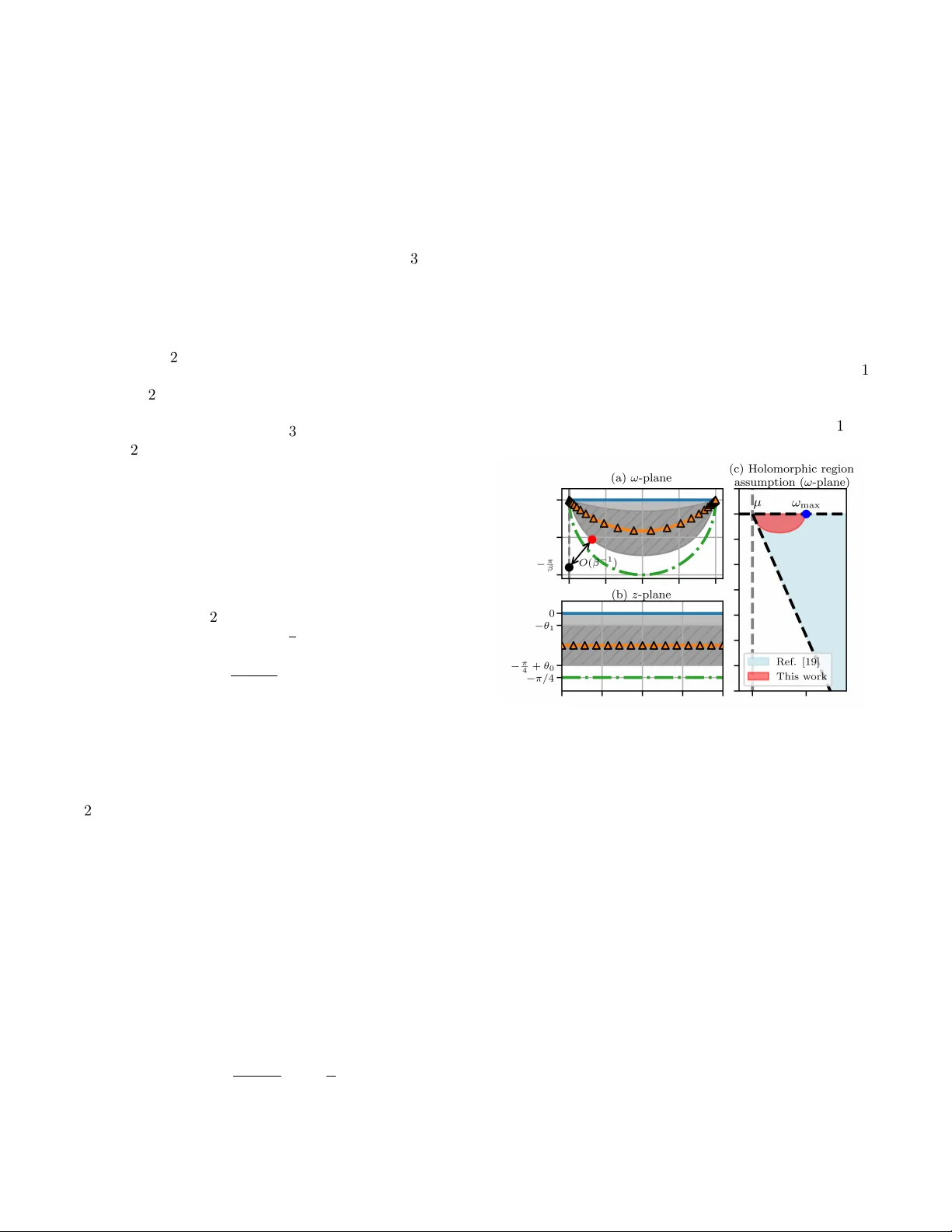
Pro v ably Ecien t Long-Time Exp onen tial Decomp ositions of Non-Mark o vian Gaussian Baths Zhen Huang, 1 Zhiy an Ding, 2 Ke W ang, 2 Jason Ka ye, 3, 4 Xian tao Li, 5 and Lin Lin 1, 6 , ∗ 1 Dep artment of Mathematics, University of California, Berkeley, CA 94720, USA 2 Dep artment of Mathematics, University of Michigan, A nn A rb or, MI 48109, USA 3 Center for Computational Quantum Physics, Flatir on Institute, New Y ork, NY 10010, USA 4 Center for Computational Mathematics, Flatir on Institute, New Y ork, NY 10010, USA 5 Dep artment of Mathematics, Pennsylvania State University, University Park, P A 16802, USA 6 Applie d Mathematics and Computational R ese ar ch Division, L awr enc e Berkeley National L ab or atory, Berkeley, CA 94720, USA (Dated: March 27, 2026) Gaussian baths are widely used to model non-Mark ovian environmen ts, yet the cost of accu- rate simulation at long times remains p o orly understoo d, esp ecially when sp ectral densities exhibit nonanalytic b ehavior as in a range of realistic mo dels. W e rigorously b ound the complexity of rep- resen ting bath correlation functions on a time interv al [0 , T ] b y sums of complex exp onen tials, as emplo yed in recent v ariants of pseudomode and hierarc hical equations of motion methods. These b ounds mak e explicit the dep endence on the maximal sim ulation time T , inv erse temperature β , and the t yp e and strength of singularities in an eectiv e sp ectral density . F or a broad class of sp ectral densities, the required n umber of exp onen tials is bounded indep endently of T , achieving time-uniform complexity . The T -dependence emerges only as p olylogarithmic factors for sp ectral densities with strong singularities, such as step discontin uities and inv erse p o wer-la w divergences. The temp erature dependence is mild for b osonic environmen ts and disappears en tirely for fermionic en vironments. Th us, the true b ottlenec k for long-time simulation is not the simulation duration itself, but rather the presence of sharp nonanalytic features in the bath sp ectrum. Our results are instructiv e b oth for long-time simulation of non-Marko vian op en quantum systems, as well as for Mark ovian em b eddings of classical generalized Langevin equations with memory kernels. Intr o duction.– The mo del of a quantum system lin- early coupled to a Gaussian environmen t is widely used across quantum optics [1, 2 ], condensed matter physics [ 3 , 4 ], and chemical and biological physics [ 5 , 6]. While Mark ovian approximations capture short-time dynamics and weak system-bath coupling, man y relev an t regimes extend b ey ond weak coupling and are intrinsically non- Mark ovian. Such non-Marko vian eects can b e captured b y pseudomo des [ 7 – 21], whic h are auxiliary degrees of freedom that repro duce the bath correlation functions (BCF s) and enable ecient simulation schemes. The computational scaling of dierent pseudomo de constructions can v ary widely , particularly for simula- tions at long sim ulation times ( T ). Hamiltonian-based pseudomo de constructions such as TEDOP A suer from p olynomial scaling with T [10, 11, 14, 15] which has b e- come an obstruction to wards practical long-time sim- ulations. Similarly , hierarchical equations of motion (HEOM) metho ds [ 6 , 16] also suer from similar pro- hibitiv e scalings in T . Recen t adv ances such as quasi- Lindblad pseudomo des [18, 19], coupled-Lindblad pseu- domo des [20, 21], and free-p ole HEOM (FP-HEOM) [17] represen t BCF s as optimized sums of exp onentials with complex w eights and p oles. This enables ecient long- time sim ulations across a wide range of physical systems. Despite their practical success, rigorous complexity analysis has only app eared recently: the sharp est av ail- ∗ linlin@math.berkeley .edu able b ounds in the analytic setting were obtained in [19] and rely on strong analyticity assumptions on the sp ec- tral density . Man y ph ysically relev ant settings do not satisfy such assumptions. F or instance, the density of states of p eriodic systems generically exhibits v an Hov e singularities [22]: inv erse p ow er-la w divergences at band edges in one dimension, logarithmic div ergences in t w o dimensions, and a square-ro ot cusp in three dimensions. Ev en within the analytic setting, existing upp er b ounds are not tight. As an illustrative example, w e consider the spin–b oson mo del with an Ohmic spectral densit y J ( ω ) = ω e − ω at zero temp erature. Figure 1 sho ws the num ber of bath mo des N required to achiev e a xed accuracy ε = 0 . 01 in the L 1 norm for repro duc- ing the bath correlation function ov er the time in terv al [0 , T ] , plotted as a function of the maximal simulation time T . F or comparison, w e include three reference scal- ings, N ∝ T , N ∝ log T , and N ∝ (log T ) 2 (the upp er b ound established for this setting in [19]). Numerical re- sults (for details, see [23, Section S5]) suggest that the required n umber of bath mo des can b e asymptotically in- dep enden t of T , which would lead to a signicant saving in simulation cost. Moreo ver, compact sum-of-exp onentials (SOE) repre- sen tations for imaginary-time functions with logarithmic scaling in inv erse temp erature hav e enabled ma jor al- gorithmic adv ances in equilibrium quantum many-bo dy calculations with rigorous complexit y estimates. Ap- proac hes such as the Discrete Lehmann Representation (DLR) [24] and p ole tting [25 – 27] hav e led to ecient 2 Sup er-Ohmic Bosonic bath Sub-Ohmic Bosonic bath Gapp ed F ermionic bath Gapless F ermionic bath Zero T emperature O  log 2  1 ω c ε  O  log 2  1 ω c ε  O  log 2  1 ω c ε  O  log  log( ω c T ) ω c ε  log  T ε   Finite T emperature O  log 2  (1 + 1 β ω c ) · 1 ω c ε  O  log 2  1 ω c ε  + log 2  1 β ω c · T ε  T ABLE I. Summary of the complexit y bounds for representing bath correlation functions of v arious physically relev ant systems, with L 1 accuracy ε on [0 , T ] . Here ω c is a characteristic frequency scale of the bath (for example, see Eq. ( 4 ) for its denition in the Ohmic-family sp ectral densities). The b ounds are indep enden t of T for sup er-Ohmic b osonic baths and gapp ed fermionic baths at all temperatures and for sub-Ohmic b osonic baths at zero temperature, and dep end on T only through p olylogarithmic factors for nite temp erature sub-Ohmic b osonic baths and gapless fermionic baths. F or simplicit y , we hav e omitted the results for Ohmic b osonic baths in this table, which are O  log 2 ( 1 ω c ε ) + log( log( ω c T ) β ω 2 c ε ) log( T β ω c ε )  . 10 10 2 10 3 T (log-scale) 3 4 5 6 7 8 9 10 N Required bath size N ∝ T N ∝ (log T ) 2 N ∝ log T FIG. 1. Num b er of bath mo des N required to represen t the bath of an Ohmic spin-b oson mo del at zero temp erature with xed accuracy ε = 0 . 01 in L 1 norm, as a function of the maxim um simulation time T . sc hemes for diagrammatics [28 – 30], analytic contin uation [26, 31], and accelerating equilibrium dynamical mean- eld theory (DMFT) [28, 29] calculations. A natural and frequently raised question is the eciency of sim- ilarly compact representations in nonequilibrium real- time calculations (such as [17, 18, 21, 32]). This work addresses that question b y establishing rigorous complex- it y b ounds. In this Letter, w e present a unied, rigorous frame- w ork for determining the simulation complexity of real- time Gaussian environmen ts. Our approach adv ances prior analyses in v arious w a ys. W e establish complex- it y b ounds that remain v alid in the presence of sp ectral singularities (see T able I ). F or many physically relev ant regimes, w e pro ve how the n umber of bath mo des N re- quired scales with maxim um simulation time T . F or xed target L 1 accuracy of the bath correlation functions on [0 , T ] , the long-time scaling dep ends on the singularit y t yp e: N is indep enden t of T for mild singularities (e.g. square-ro ot); N = O (log T log log T ) for step discontin u- ities or logarithmic singularities; and, in the worst case, N = O ((log T ) 2 ) for in verse p ow er-la w divergences. Setup.– A Gaussian environmen t is describ ed by its sp ectral density J ( ω ) , which is a non-negative, piecewise smo oth L 1 function that is compactly supp orted or ex- p onen tially decaying. The lesser and greater bath cor- relation functions (for fermionic problems, they are also kno wn as hybridization functions) are: ∆ < ( t ) = Z ∞ −∞ J ( ω ) f ( ω − µ ) e − i ω t d ω , ∆ > ( t ) = Z ∞ −∞ J ( ω )  1 ± f ( ω − µ )  e − i ω t d ω . (1) Here f ( ω ) is the Bose–Einstein function f BE ( ω ) = 1 e β ω − 1 for b osonic baths, and the F ermi–Dirac function f FD ( ω ) = 1 e β ω +1 for fermionic baths; the sign + corre- sp onds to bosons and − to fermions. β is the inv erse temp erature and µ is the c hemical potential. F or bosonic problems, µ should lie b elow the b ottom of the supp ort of J ( ω ) (or, if µ coincides with a band edge, that J ( ω ) v anishes suciently fast there) to av oid a divergen t o c- cupation; it is conv en tional to set µ = 0 and take J supp orted on [0 , ∞ ) . F or b osonic baths we work with the total BCF ∆( t ) = ∆ > ( t ) + ∆ < ( − t ) = Z ∞ −∞ J e ( ω ) e − i ω t d ω , (2) with J e ( ω ) = sign( ω ) J ( | ω | ) 1 − e − β ω . F or fermions, set J < e ( ω ) = J ( ω ) f FD ( ω − µ ) and J > e ( ω ) = J ( ω )[1 − f FD ( ω − µ )] so that ∆ >,< ( t ) = R ∞ −∞ J >,< e ( ω ) e − i ω t d ω . Here f FD is the F ermi–Dirac function. In what follows, we will omit the >, < sup erscript since the analysis holds for b oth cases. T o nd a compact representation of the bath, our goal is to approximate ∆( t ) b y a sum of exp onen tials: ∆( t ) = N X j =1 c j e − i z j t + δ ( t ) , t ∈ [0 , T ] , (3) suc h that the error δ ( t ) is small. W e say the approxima- tion on [0 , T ] has ε accuracy in L 1 norm if R T 0 | δ ( t ) | d t ≤ ε . A ccording to [12, 33], controlling the L 1 b ound allows us to control errors of any b ounded system observ ables. Th us the problem of simulating Gaussian environmen ts reduces to approximating BCF s by sums of exp onen tials with controlled errors. 3 Conformal mapping and exp onential ly clustering p oles. Giv en J e ( ω ) , we will treat the frequency domain ω > µ and ω < µ separately . If J e ( ω ) is not analytic globally but only piecewise analytic, w e will also consider eac h an- alytic segmen t separately . The o v erall complexit y is then the sum of the complexities for each analytic segmen t, whic h is dominated b y the segment with the strongest singularit y . In what follo ws, w e use the terms exp onents , p oles , and quadr atur e no des interc hangeably , as they all refer to the same quantities z j ’s dened in Eq. ( 3 ). The k ey idea of our analysis is illustrated in Fig. 2. F or each smo oth segment of J e ( ω ) , we assume it ad- mits a holomorphic extension to a sub domain Ω of the semi-circular region in the low er half-plane (the gra y re- gion in Fig. 2 (a)). W e note that this is a muc h weak er analyticit y assumption compared to previous works [19] (see Fig. 2 (c) for comparison). T o resolve p ossible end- p oin t singularities of each analytic segmen t, w e place quadrature no des z j ’s in Eq. ( 3 ) (illustrated as triangles in Fig. 2 (a)) in the low er half-plane that are exponentially clustered tow ard the segment endp oin ts. Suc h c hoice of { z j } can b e viewed as dening a nonuniform quadra- ture rule for integration along a contour deformed in to the low er half-plane. In the Supp ort Information (SM) [23, Section S2], we show that suc h a choice achiev es the desired accuracy using a conformal map that sends the semi-elliptic region to a strip in the low er complex plane, in which the corresp onding quadrature no des are uniform (see Fig. 2 (b)). Moreov er, the analytic region guaran tees that there is an O ( 1 β ) distance from the p oles of the F ermi-Dirac functions, which are the Matsubara frequencies ν n = µ − i π (2 n +1) β . This property is crucial in pro ving the asymptotic β -indep endence of the required n umber of p oles for fermionic baths. As noted earlier, the complexity (i.e., the num b er of exp onen tially clustered poles required near eac h singu- larit y) dep ends on the strength of the singularity . This dep endence is rigorously form ulated in SM [23, Corollary 2 ] and in [23, Eq. (S5)], which we summarize b elo w. In essence, the required num b er of p oles scales logarithmi- cally with a prefactor related to the L 1 norm of the bath correlation function (see [23, Section S2]). F or weak sin- gularities, such as J e ( ω ) ∼ | ω − ω 0 | α with α > 0 , its F ourier transform decays faster than 1 /t and is there- fore L 1 in tegrable on [0 , ∞ ) , leading to a T -indep endent complexit y: O (log 2 (1 /ω c ε )) . Here ω c is the c haracter- istic frequency scale of the bath. In con trast, for a stronger singularit y such as an in verse p ow er-la w b eha v- ior J e ( ω ) ∼ | ω − ω 0 | − α with 0 < α < 1 , the hybridiza- tion function decays slow er than 1 /t , and the complexity is p olylogarithmic in T : O (log 2 ( T /ε )) . F or in termediate singularities such as step or logarithmic singularities, the complexit y is O  log  log( ω c T ) ω c ε  log  T ε   . W e refer to SM [23, Section S1] for precise denitions of singularit y t yp es and [23, Section S2] for detailed rigorous pro ofs. log 2 T -dep endenc e in a pr e-asymptotic r e gime. W e fo- cus on the asymptotic scaling of the required num b er of bath mo des N with resp ect to the maximum simulation time T . F or mild singularities J e ( ω ) ∼ | ω − ω 0 | α with α > 0 , the asymptotic b ound is T -indep enden t b ecause the L 1 norm of the tail is uniformly b ounded as T → ∞ . Therefore, once the approximation is made sucien tly accurate on [0 , T ∗ ] , where the tail R ∞ T ∗ | ∆( t ) | d t is su- cien tly small, that approximation remains v alid to within the sp ecied tolerance ε for all later times. Of course, this threshold time increases as ε decreases, whic h accounts for the ε -dep endence app earing in all of the complexity results. W e note that this T -indep endence eect do es not preclude an intermediate regime b efore saturation in whic h the minimal num ber of p oles still grows with T ; in practice this gro wth can resem ble log T , as seen in Fig. 1 . Th us the asymptotic T -indep enden t complexity for mild singularities is consisten t with the pre-asymptotic behav- ior often observed in computations, including Fig. 1 . FIG. 2. (a,b) Contour transformation from the ω -plane to the z -plane. The gray area is the holomorphic region Ω of J e ( ω ) , and the hatched area is the analyticity strip used in our analysis. Corresp onding contours are illustrated in the same color. (c) Comparison of the holomorphic region in our analysis and that in Ref. [19]. T emp er atur e indep endenc e. The temp erature depen- dence of the BCF s enters through Bose-Einstein or F ermi- Dirac functions in the eectiv e sp ectral density , af- fecting the prefactor of exp onential conv ergence. The F ermi-Dirac function is b ounded in the analyticity re- gion, so the prefactor (and the nal complexity) is β - indep enden t for fermionic systems. F or b osonic systems, the Bose-Einstein function diverges at ω = 0 , leading af- ter nondimensionalization to a prefactor that scales as O (1 + 1 / ( β ω c )) and hence only logarithmic dep endence on temp erature in the nal complexit y . In the physically relev ant regime β ω c ≳ 1 , this prefactor remains O (1) . F or details, see the SM [23, Section S3]. Sub-Ohmic, Ohmic and Sup er-Ohmic b osonic b aths. The rst ph ysical example is the Ohmic family of sp ec- 4 (a) (b) DOS N v .s. T μ μ DOS N v .s. T (c) Singularity 1D 2D 3D, partially filled 3D, fully filled Inverse square root Logarithmic Step discontinuity Continuous (Non-smooth) Singularity Step discontinuity Continuous (Non-smooth) FIG. 3. (a) A system coupled to a fermionic p erio dic lattice. (b) Sp ectral density in the case of 1D, 2D and 3D lattices exhibiting the v an Hov e singularities, and corresp onding complexity scalings in T . (c) Gapless and gapp ed sp ectral densities with p ow er-la w singularities at the band edge, and corresp onding complexity scalings in T . tral densities, whic h has been widely used to model ligh t- matter interactions and quan tum dissipation for decades [34]. The sp ectral density is given by J ( ω ) = ω γ ω − ( γ +1) c e − ω /ω c , ω ∈ [0 , ∞ ) , γ > 0 . (4) F or γ > 1 , J is said to be sup er-Ohmic, γ = 1 is Ohmic, and γ < 1 is sub-Ohmic. Consider a contin uous cuto function χ W ( ω ) that is compactly supp orted on [0 , W ] : χ W ( ω ) =    1 − e − ( W − ω ) /ω c 1 − e − W/ω c , ω ∈ [0 , W ] , 0 , ω ∈ [ W, ∞ ) . W e choose a large enough W suc h that J ( ω ) is very close to J trunc ( ω ) = J ( ω ) χ W ( ω ) . This nite truncation argu- men t could b e made rigorous by carefully b ounding the L 1 truncation error (see SM [23, Prop osition 2 ]). A t zero temp erature, w e can see that since γ > 0 , J e ( ω ) = J ( ω ) χ W ( ω ) has singularit y order γ at ω = 0 and singularit y order 1 at ω = W . Thus the ov erall sin- gularit y order is α = min { γ , 1 } , and the complexit y is indep enden t of T for all Ohmic families. At nite tem- p erature, how ev er, there are qualitative dierences for dieren t regimes of γ . Since J e ( ω ) ∼ | ω | γ − 1 /β as ω → 0 , the singularity order b ecomes α = min { γ − 1 , 1 } . Thus the sup er-Ohmic, Ohmic and sub-Ohmic cases each ex- hibit qualitativ ely dierent complexity scalings in T for L 1 accuracy: no T -dep endence for sup er-Ohmic baths, N ∼ O (log( T /ε ) log(log( T ) /ε )) for Ohmic baths, and N ∼ O ((log ( T /ε )) 2 ) for sub-Ohmic baths. T o the b est of our knowledge, this is the rst rigorous complexit y b ound that applies across the Ohmic family while distinguishing the sup er-Ohmic, Ohmic, and sub- Ohmic regimes through their dierent T -dep endences. Our result, as summarized in T able I , th us provides a no vel theoretical persp ective on ho w these regimes dier: the T -dep endence of the bath-representation complexity is qualitativ ely distinct in the sub-Ohmic, Ohmic, and sup er-Ohmic cases. V an Hove singularities. Next, let us consider a sys- tem coupled to an n -dimensional p erio dic lattice, which is a tight-binding lattice of noninteracting electrons, as illustrated in Fig. 3 (a). The sp ectral densit y ex- hibits the dimension-dependent v an Hov e singularities considered ab ov e (Fig. 3 (b)), all of which are cov ered b y our analysis. In 1D, the sp ectral density has in- v erse square-ro ot singularities at the band edges, namely J e ( ω ) ∼ | ω − ω 0 | − 1 / 2 , pro ducing the w orst-case scal- ing N = O  log 2 ( T /ε )  . In 2D, the logarithmic sin- gularit y J e ( ω ) ∼ log | ω | and the step discon tin uit y at the band edge both giv e the in termediate scaling N = O  log( T /ε ) log log ( T /ε )  . In 3D, if the band is partially lled, the jump discontin uit y at the c hemical potential µ leads to the O (log( T /ε ) log log( T /ε )) scaling. Other- wise, if the band is fully lled, then the complexity is T -indep endent. Gapless and gapp e d b aths. As a nal example, let us illustrate the qualitativ e dierence b et ween gapless and gapp ed spectral densities for long-time simulation. As sho wn in Fig. 3 (c), the gapp ed sp ectral density v anishes con tinuously at ω = µ and thus has singularity order α > 0 . F or a gapless bath at nite temp erature, the ther- mal eective sp ectral density is itself smo oth at ω = µ . Ho wev er, to obtain a represen tation whose complexit y is uniform in β , we split the frequency domain at µ and treat the tw o sides separately , as describ ed ab o ve. In this segmented representation the b oundary p oint ω = µ b eha v es as an endpoint singularit y of order α = 0 . By T a- ble I , repro ducing the BCF s for a gapp ed bath requires a num b er of mo des indep enden t of T , while a gapless bath demands bath mo des with size gro wing p olylog- arithmically in T . This p olylogarithmic T -dep endence should therefore b e understoo d as the cost of enforcing β - indep enden t complexity for a gapless bath, rather than as a physical nonanalyticity of the nite-temp erature sp ec- trum itself. F or xed β , one may instead exp ect to re- co ver T -indep endent complexit y by analyzing the smo oth thermal eective sp ectral density directly , but then the resulting constants would no longer remain uniform as β decreases. A pplic ability to classic al op en systems. Although our primary motiv ation is to characterize the complexity of op en quantum systems, the challenge of nding compact bath representations is universal. In classical molecu- lar dynamics, the Generalized Langevin Equation (GLE) go verns the system dynamics, where the memory kernel is in trinsically determined b y en vironmental noise uctu- 5 ations via the uctuation-dissipation theorem. Crucially , when this memory kernel is accurately represented by a compact sum of exp onentials, the GLEs, which are non- lo cal in time, map exactly on to a system of local auxiliary dieren tial equations [35 – 37]. In particular, the conv o- lution in tegral with an exp onen tial kernel can b e recast as a simple dierential equation, eectiv ely eliminating the need to store the history . This transformation re- duces the simulation complexity from quadratic in time T to linear. Such embeddings hav e pro ven essential for capturing complex memory eects in visco elastic phe- nomena, protein folding, and hydration dynamics [38– 40]. W e refer the reader to the SM [ 23, Section S4] for sp ecic examples where sp ectral singularities naturally arise in these classical contexts. Conclusions and outlo ok. In this Letter, w e hav e dev elop ed a general theoretical framew ork for analyz- ing the complexit y of simulating Gaussian environmen ts with general sp ectral densities. Our result systemati- cally characterizes the complexity for dierent singular- it y t yp es. This establishes a rigorous foundation for both recen tly developed quasi-Lindblad pseudomo de metho ds [19, 33] and the free-pole HEOM methods [17], as well as Marko vian embedding approaches in classical molecu- lar dynamics with memory kernels, precisely quantifying their complexity for long-time sim ulations at low tem- p eratures. This work also op ens up several interesting directions for future research. Based on our results, we ma y ex- tend prior analysis of tensor net work inuence function- als [41] b ey ond the Ohmic case to sup er-Ohmic and sub- Ohmic sp ectral densities. Though our analysis could b e straigh tforwardly extended to multi-band systems, it re- mains unclear what the optimal complexity is in terms of the num ber of bands. Moreov er, it is also unclear how to dev elop a similar complexity result for the more re- cen t coupled-Lindblad pseudomode theories [21], which satisfy additional constraints to guarantee physicalit y of the system dynamics. A cknow le dgements. This material is based up on work supp orted by the Simons T argeted Gran t in Mathematics and Physical Sciences on Moiré Materials Magic (Z.H., L.L.), by the U.S. Department of Energy , Oce of Sci- ence, A ccelerated Researc h in Quan tum Computing Cen- ters, Quantum Utilit y through Adv anced Computational Quan tum Algorithms, grant no. DE-SC0025572 (L.L.), b y a startup gran t from the Universit y of Michigan (Z.D., K.W.), by the V an Lo o Postdoctoral F ellowship (K.W.), and by the NSF Grant CCF-2312456 (X.L.). L.L. is a Simons Inv estigator in Mathematics. The Flatiron Insti- tute is a division of the Simons F oundation. W e thank Andrew Millis, Olivier Parcollet, Steven White, and Ma- ciej Zworski for helpful discussions. [1] A. Riv as and S. F. Huelga, Op en quantum systems , V ol. 10 (Springer, 2012). [2] P . F orn-Díaz, L. Lamata, E. Rico, J. Kono, and E. Solano, Reviews of Modern Ph ysics 91 , 025005 (2019). [3] A. Georges, G. Kotliar, W. Krauth, and M. J. Rozen b erg, Reviews of mo dern physics 68 , 13 (1996). [4] R. Haertle, G. Cohen, D. Reichman, and A. Millis, Phys- ical Review B 88 , 235426 (2013). [5] S. Mukamel and D. Abramavicius, Chemical Reviews 104 , 2073 (2004). [6] M. T anaka and Y. T animura, Journal of the Physical So ciet y of Japan 78 , 073802 (2009). [7] B. Garraw a y , Physical Review A 55 , 2290 (1997). [8] A. Dorda, M. Nuss, W. v on der Linden, and E. Arrigoni, Ph ys. Rev. B 89 , 165105 (2014). [9] A. Dorda, M. Ganahl, H. G. Ev ertz, W. von der Linden, and E. Arrigoni, Ph ys. Rev. B 92 , 125145 (2015). [10] M. P . W o o ds and M. B. Plenio, Journal of Mathematical Ph ysics 57 (2016). [11] R. Rosen bach, J. Cerrillo, S. F. Huelga, J. Cao, and M. B. Plenio, New Journal of Physics 18 , 023035 (2016). [12] F. Mascherpa, A. Smirne, S. F. Huelga, and M. B. Plenio, Ph ysical review letters 118 , 100401 (2017). [13] D. T amascelli, A. Smirne, S. F. Huelga, and M. B. Plenio, Ph ysical review letters 120 , 030402 (2018). [14] D. T amascelli, A. Smirne, J. Lim, S. F. Huelga, and M. B. Plenio, Physical review letters 123 , 090402 (2019). [15] A. Nüßeler, I. Dhand, S. F. Huelga, and M. B. Plenio, Ph ysical Review B 101 , 155134 (2020). [16] Y. T animura, The Journal of Chemical Ph ysics 153 , 020901 (2020). [17] M. Xu, Y. Y an, Q. Shi, J. Ank erhold, and J. Sto ckburger, Ph ysical Review Letters 129 , 230601 (2022). [18] G. Park, Z. Huang, Y. Zhu, C. Y ang, G. K.-L. Chan, and L. Lin, Physical Review B 110 , 195148 (2024). [19] J. Thoenniss, I. Vilko viskiy , and D. A. Abanin, arXiv preprin t arXiv:2409.08816 (2024). [20] M. Lednev, F. J. García-Vidal, and J. F eist, Physical Review Letters 132 , 106902 (2024). [21] Z. Huang, G. Park, G. K. Chan, and L. Lin, Phys. Rev. Lett. in press (2026). [22] L. V an Hov e, Physical Review 89 , 1 189 (1953). [23] See supplemental material for mathematical details, whic h includes refs. [42 – 44]. [24] J. Kay e, K. Chen, and O. Parcollet, Physical Review B 105 , 155115 (2022). [25] Y. Nakatsukasa, O. Sète, and L. N. T refethen, SIAM Journal on Scientic Computing 40 , A1494 (2018). [26] Z. Huang, E. Gull, and L. Lin, Physical Review B 107 , 075151 (2023). [27] L. Ying, Journal of Scientic Computing 92 , 107 (2022). [28] J. Kay e, Z. Huang, H. U. Strand, and D. Golež, Physical Review X 14 , 031034 (2024). [29] Z. Huang, D. Golež, H. U. Strand, and J. Kay e, arXiv preprin t arXiv:2503.19727 (2025). [30] D. Gazizo v a, L. Zhang, E. Gull, and J. LeBlanc, Physical Review B 110 , 075158 (2024). [31] L. Zhang, Y. Y u, and E. Gull, arXiv preprint arXiv:2410.14000 (2024). [32] L. Zhang, A. Erpenbeck, Y. Y u, and E. Gull, The Journal of Chemical Physics 162 (2025). 6 [33] Z. Huang, L. Lin, G. Park, and Y. Zhu, arXiv preprint arXiv:2411.08741 (2024). [34] A. J. Leggett, S. Chakrav arty , A. T. Dorsey , M. P . Fisher, A. Garg, and W. Zw erger, Reviews of Mo dern Physics 59 , 1 (1987). [35] P . Siegle, I. Goyc h uk, P . T alkner, and P . Hänggi, Phys- ical Review E—Statistical, Nonlinear, and Soft Matter Ph ysics 81 , 011136 (2010). [36] I. Goyc h uk, Adv ances in Chemical Ph ysics 150 , 187 (2012). [37] R. Kupferman, Journal of statistical physics 114 , 291 (2004). [38] B. A. Dalton, C. A yaz, H. Kiefer, A. Klimek, L. T epp er, and R. R. Netz, Pro ceedings of the National Academ y of Sciences 120 , e2220068120 (2023). [39] G. Jung, M. Hanke, and F. Schmid, Journal of chemical theory and computation 13 , 2481 (2017). [40] J. O. Daldrop, B. G. Ko w alik, and R. R. Netz, Physical Review X 7 , 041065 (2017). [41] I. Vilko viskiy and D. A. Abanin, Physical Review B 109 , 205126 (2024). [42] S. Adelman and J. D. Doll, The Journal of Chemical Ph ysics 61 , 4242 (1974). [43] E. Lutz, Physical Review E 64 , 051106 (2001). [44] R. Roy and T. Kailath, IEEE T ransactions on Acoustics, Sp eec h, and Signal Pro cessing 37 , 984 (1989). [45] L. N. T refethen and J. W eideman, SIAM review 56 , 385 (2014). Supp ort Information for Long-time sim ulation of general non-Mark o vian Gaussian en vironmen ts at arbitrary temp erature: theoretical analysis Zhen Huang 1 , Zhiyan Ding 2 , Ke W ang 2 , Jason Kay e 3 , 4 , Xiantao Li 5 and Lin Lin 1 , 6 1 Dep artment of Mathematics, University of California, Berkeley, CA 94720, USA 2 Dep artment of Mathematics, University of Michigan, A nn A rb or, MI 48109, USA 3 Center for Computational Quantum Physics, Flatiron Institute, New Y ork, NY 10010, USA 4 Center for Computational Mathematics, Flatir on Institute, New Y ork, NY 10010, USA 5 Dep artment of Mathematics, Pennsylvania State University, University Park, P A 16802, USA 6 Applie d Mathematics and Computational R ese ar ch Division, L awr ence Berkeley National L ab oratory, Berkeley, CA 94720, USA (Dated: March 27, 2026) S1. SETUP In this section, w e review the problem setup and p erform the nondimensionalization. Recall that in the main text, the BCF is the F ourier transform of the eective sp ectral density J e ( ω ) : ∆( t ) = Z ∞ −∞ J e ( ω ) e − iω t d ω , where J e ( ω ) is given by the sp ectral density J ( ω ) through the following relation: J e ( ω ) = sign( ω ) J ( | ω | ) 1 − e − β ω . F or b osons. J < e ( ω ) = J ( ω ) f FD ( ω − µ ) , J > e ( ω ) = J ( ω )(1 − f FD ( ω − µ )) , F or fermions. Here J ( ω ) is the sp ectral density , which is compactly supp orted or decays exp onen tially fast. As describ ed in the main text, we treat each analytic segmen t of J e ( ω ) separately . F or fermions, we also treat the domains ω > µ and ω < µ separately , where µ is the chemical p otential ( µ is zero for b osons). Thus w e assume that J e ( ω ) is supp orted on [ ω a , ω b ] and is analytic in the semi-ellipse b elo w [ ω a , ω b ] , as illustrated in Fig. 2 (a) (the dark grey area). F or now, w e assume that ω a and ω b are nite, and we discuss how to truncate innite domains in Section S3. Nondimensionalization T o nondimensionalize, dene ω ′ , the rescaled frequency that maps [ ω a , ω b ] to [ − 1 , 1] : ω ′ = 2 ω − ( ω a + ω b ) ω b − ω a , ω ∈ [ ω a , ω b ] , ω ′ ∈ [ − 1 , 1] . Dene the rescaled sp ectral densities e J ( ω ′ ) = ω b − ω a 2 J ( ω ) , e J e ( ω ′ ) = ω b − ω a 2 J e ( ω ) . Then the F ourier transform of e J e ( ω ′ ) , denoted b y e ∆( t ) , satises e ∆  ω b − ω a 2  t  = e i ω a + ω b 2 t ∆ ( t ) . T o achiev e L 1 error less than ε for ∆( t ) on [0 , T ] , it suces to achiev e L 1 error less than W ε for e ∆( t ) on [0 , W T ] , where W = ω b − ω a 2 is the half bandwidth. Note that since ε is the L 1 error for ∆( t ) , it has the dimension of time. Th us W ε and W T are dimensionless quantities. In the following, we work with the rescaled quantities ω ′ ∈ [ − 1 , 1] and drop t he tilde and prime for simplicity . 2 Con tour deformation, change of v ariables and analyticity assumptions A k ey step in our analysis is the c hange of v ariables ω = tanh x , whic h maps the domain ω ∈ [ − 1 , 1] to x ∈ [ −∞ , ∞ ] . Then we hav e: ∆( t ) = Z + ∞ −∞ J e (tanh x )e − i t tanh x 1 cosh 2 x d x. Let us dene g ( z ; t ) = J e (tanh z )e − i t tanh z 1 cosh 2 z , (S1) as the complexication of the integrand, for Im( z ) ∈ [ − π 4 + θ 0 , 0] . Here θ 0 > 0 . Then, by contour deformation, we can ev aluate ∆( t ) by integrating along the line Im z = − y for any y ∈ [0 , π 4 − θ 0 ] : ∆( t ) = Z + ∞ −∞ g ( x − i y ; t ) d x, ∀ y ∈ [0 , π 4 − θ 0 ] . (S2) As shown in Section S2, we will consider y = − Im( z ) ∈ [ θ 1 , π 4 − θ 0 ] for some nonzero θ 1 to take adv an tage of the deca y prop erties in t . In other w ords, g ( z ; t ) is required to b e analytic in the strip S : S = { z : Im z ∈ [ − π 4 + θ 0 , − θ 1 ] } . (S3) Th us we make the follo wing analyticity assumption on J e ( ω ) : Assumption 1. J e ( ω ) is analytic in the following semi-ellipse Ω b elow [ − 1 , 1] : Ω = { ω : ω = tanh z , Im z ∈ [ − π 4 + θ 0 , 0] } . Here θ 0 ∈ (0 , π 4 ) is a constant. The region Ω is illustrated in Fig. 2 (a) (the dark grey area). Since we can alwa ys restrict to a smaller holomorphic region, without loss of generality , w e may assume that J eff ( ω ) is analytic on Ω except at ω = ± 1 . Singularit y order α In the main text we ha v e formally introduced the notion of singularity order α to c haracterize the singularity b eha vior of J e at its endp oint ω = ± 1 . Here we give a more precise denition. Denition 1 (Singularity order α ) . F or α > − 1 and α  = 0 , w e say a function f ( ω ) has a singularity of order α at ω = 1 if there exists C > 0 such that | f ( ω ) | ≤ C | ω − 1 | α as ω → 1 within Ω , while for every α ′ > α , | f ( ω ) | | ω − 1 | α ′ is un b ounded. F or α = 0 , we require instead that there exists C > 0 such that | f ( ω ) | ≤ C (1 + | log | ω − 1 || ) as ω → 1 within Ω , and that for every α ′ > 0 , | f ( ω ) | | ω − 1 | α ′ is unbounded. This class includes both logarithmic singularities and b ounded jump discon tinuities. A similar denition applies to the singularity at ω = − 1 . F or f ( ω ) with singularity order α ± at ω = ± 1 , we dene α = min { α + , α − } as the ov erall singularity order. With this denition, after p ossibly enlarging the constan t to accoun t for the compact part of Ω aw a y from the endp oin ts, there exists C J > 0 such that the corresp onding endp oint b ounds hold on the t wo half-domains. Let Ω + = { ω ∈ Ω : Re ω ≥ 0 } , Ω − = { ω ∈ Ω : Re ω ≤ 0 } . More precisely , J e ( ω ) of singularity order α satises the b ounds | J e ( ω ) | ≤ C J | ω − 1 | α , for ω ∈ Ω + , α > − 1 , α  = 0 , | J e ( ω ) | ≤ C J | ω + 1 | α , for ω ∈ Ω − , α > − 1 , α  = 0 , | J e ( ω ) | ≤ C J (1 + | log( | ω − 1 | ) | ) , for ω ∈ Ω + , α = 0 , | J e ( ω ) | ≤ C J (1 + | log( | ω + 1 | ) | ) , for ω ∈ Ω − , α = 0 . (S4) 3 S2. MAIN RESUL T Our main result is based on the following theorem, which gives a p oin twise estimate on the error of approximating ∆( t ) by a sum of exp onen tials. Theorem 1 (Poin twise error estimate) . Suppose that the eective sp ectral function J e ( ω ) has singularit y of order α > − 1 at ω = ± 1 (see Denition 1 ). Then there exist constan ts A α , c > 0 , indep enden t of t , and a choice of y 2 ∈ ( θ 1 , π 4 − θ 0 ) such that for any 0 < h < 1 , M > 1 , and t ≥ 0 , we hav e       ∆( t ) − X | nh |≤ M hg ( nh − i y 2 ; t )       ≤ C J · ( A α (e − c/h (1 + t ) − (1+ α ) + j M ,α ( t )) , α  = 0 , α > − 1 A 0  e − c/h log(2+ t ) 1+ t + j M , 0 ( t )  , α = 0 . Here j M ,α ( t ) = min { e − ( α +1) M , (1 + t ) − (1+ α ) } for α  = 0 , j M , 0 ( t ) = e − M , and C J is the mo del-dependent constant in Eq. ( S4). As shown in Theorem 1 , the appro ximation of ∆( t ) = R ∞ −∞ g ( x − i y ; t ) d x is given b y a uniform discretization in x with step size h and truncation | x | < M , for a xed y . W e leav e the pro of of Theorem 1 to the end of this section. Note that the tail b ound for α = 0 can b e impro ved to j M , 0 ( t ) = min(e − M , log 2 (2+ t ) 1+ t ) , but using j M , 0 ( t ) = e − M is sucien t for this work. The p oin twise error estimate in Theorem 1 directly leads to the main result of this work, whic h is the L 1 error estimate for approximating ∆( t ) : Corollary 2 (Main result: L 1 error estimate) . With the same assumptions as in Theorem 1 , to achiev e L 1 error less than ε for appro ximating ∆( t ) by a sum of exp onentials, the num b er of terms required satises the following scaling: N = O  log 2 ( C J /ε )  , for α > 0 , N = O  log  C J log( T ) ε  log  C J T ε   , for α = 0 , N = O  log 2 ( C J T /ε )  , for − 1 < α < 0 . In unrescaled quantities, T and ε should b e replaced by W T and W ε resp ectively . Thus the scaling b ecomes (omitting the C J factor): N = O  log 2 (1 /W ε )  , for α > 0 , N = O  log  log( W T ) W ε  log  T ε   , for α = 0 , N = O  log 2 ( T /ε )  , for − 1 < α < 0 . (S5) Corollary 2 leads to the main conclusion of this work in T able I , for which we hav e rescaled the quantities back to the original scale, and explicitly considered C J ’s dep endence on β , the latter of which is addressed in Section S3. W e ha ve also replaced W with the characteristic frequency ω c , which is straigh tforward for sp ectral densities with nite supp ort, and for sp ectral densities with innite supp ort but exp onen tial decay , this is also addressed in Section S3. The pro of of Theorem 2 from Theorem 1 is simply to in tegrate the p oint wise error estimate ov er t ∈ [0 , T ] , and c ho ose M and h to b ound b oth terms in the p oin t wise error estimate by ε . The details are given b elow. Pr o of of Cor ol lary 2 fr om The or em 1. F or α > 0 , by decomp osing the integral into [0 , e M ] and [e M , T ] , and using the tw o bounds e − ( α +1) M and (1 + t ) − (1+ α ) corresp ondingly for the tw o interv als, we hav e that R T 0 | j M ,α ( t ) | d t ≤ α +1 α e − αM . Thus using Theorem 1 , the L 1 error is b ounded by C J  A α α e − c/h + A α ( α +1) α e − αM  . By choosing M = 1 α log  2( α +1) C J A α αε  , 1 /h = 1 c log  2 C J A α αε  , the L 1 error is less than ε , and the n umber of terms N = ⌈ 2 M /h ⌉ = O (log 2 ( C J /ε )) . F or α < 0 , since R T 0 (1 + t ) − (1+ α ) d t = ((1 + T ) | α | − 1) / | α | , we hav e that the L 1 error is b ounded b y C J  A α | α | e − c/h (1 + T ) | α | + A α T e − ( α +1) M  . T o make this b ounded by ε , w e can choose M = 1 α +1 log  2 C J A α T ε  , 1 /h = 1 c log  2 C J A α (1+ T ) | α | | α | ε  . Th us N = ⌈ 2 M /h ⌉ = O (log 2 ( C J T /ε )) . 4 Finally , for α = 0 , since R T 0 log(2+ t ) 1+ t ≤ 2 R T 0 log(2+ t ) 2+ t d t ≤ (log(2 + T )) 2 , the L 1 error is b ounded b y C J  A 0 2 e − c/h (log(2 + T )) 2 + A 0 T e − M  . Th us, it suces to choose M = log  2 C J A 0 T ε  , 1 /h = 1 c log  2 C J A 0 (log(2+ T )) 2 ε  . W e conclude that N = ⌈ 2 M /h ⌉ = O  log  C J log( T ) ε  log  C J T ε  . Another consequence of Theorem 1 is the following L ∞ error estimate, which is T -indep endent for all α > − 1 : Corollary 3 ( L ∞ error estimate) . With the same assumptions as in Theorem 1 , to achiev e L ∞ error less than ε ∞ for approximating ∆( t ) by a sum of exp onentials, the num ber of terms required satises the following scaling: N = O  log 2 ( C J /ε ∞ )  for all α > − 1 . Pr o of of Cor ol lary 3 fr om The or em 1. By Theorem 1 , the L ∞ error is b ounded b y C J · A α (e − c/h + e − ( α +1) M ) for α  = 0 and b y C J · A 0 (e − c/h + e − M ) for α = 0 . Thus by c ho osing M = 1 α +1 log  2 C J A α ε ∞  and 1 /h = 1 c log  2 C J A α ε ∞  when α  = 0 , and M = log  2 C J A 0 ε ∞  and 1 /h = 1 c log  2 C J A 0 ε ∞  when α = 0 , the L ∞ error is less than ε ∞ , and in b oth cases N = ⌈ 2 M /h ⌉ = O (log 2 ( C J /ε ∞ )) . No w let us give a pro of of Theorem 1. The error estimate in Theorem 1 has tw o parts: the discretization error on an innite grid of size h and the truncation error on [ − M , M ] . Both errors are controlled by the decay prop erties of g ( z ; t ) in the strip S , as stated in the following lemma: Lemma 1 (Upp er b ound of g ( x − i y ; t ) (Eq. (S1))) . Given a singularity order α > − 1 of J e ( ω ) , the following upp er b ound holds for an y t ≥ 0 and y ∈ [ θ 1 , π 4 − θ 0 ] : | g ( x − i y ; t ) | ≤ C J  C α p α ( x ; t ) , α > − 1 , α  = 0 , C 0 (1 + | x | ) p 0 ( x ; t ) , α = 0 . where p α ( x ; t ) (for α > − 1 ) are dened as p α ( x ; t ) = e − c θ 1 t cosh 2 x cosh − 2( α +1) x, (S6) and C α is a constant that only dep ends on α , C J is the constan t in Eq. (S4), and c θ 1 = sin(2 θ 1 ) / 2 > 0 . Pr o of of L emma 1. Let z = x − i y . Recall that g ( z ; t ) = J e (tanh z )e − i t tanh z 1 cosh 2 z . Since | y | < π 4 , | cosh z | 2 = cosh 2 x cos 2 y + sinh 2 x sin 2 y ≥ 1 2 cosh 2 x . Therefore | 1 / cosh 2 z | ≤ 2 cosh − 2 x . Next, w e b ound e − i t tanh z . Note that | e − i t tanh z | = e t Im(tanh z ) , and Im(tanh( x − i y )) = − sin 2 y 2(sinh 2 x +cos 2 y ) . Using that y ∈ [ θ 1 , π 4 − θ 0 ] , w e ha ve − sin 2 y ≤ − sin 2 θ 1 < 0 , and sinh 2 x + cos 2 y ≤ sinh 2 x + 1 = cosh 2 x . Th us | e − i t tanh z | ≤ e − c θ 1 t/ cosh 2 x , where c θ 1 = sin(2 θ 1 ) / 2 > 0 . T o pass from the endp oin t b ounds in Eq. (S4) to a b ound on J e (tanh z ) , note that Re(tanh( x − i y )) = sinh(2 x ) cosh(2 x ) + cos(2 y ) , so the sign of Re(tanh z ) is the sign of x . Hence ω = tanh z lies in Ω + for x ≥ 0 and in Ω − for x ≤ 0 . Moreov er, 1 − tanh z = e − z cosh z , 1 + tanh z = e z cosh z . Since 2 − 1 / 2 cosh x ≤ | cosh z | ≤ cosh x when | y | < π / 4 , for x ≥ 0 we obtain 2 1 + e 2 x ≤ | ω − 1 | ≤ 2 √ 2 1 + e 2 x , 5 and similarly for x ≤ 0 , 2 1 + e − 2 x ≤ | ω + 1 | ≤ 2 √ 2 1 + e − 2 x . These quantities are comparable to cosh − 2 x up to absolute constan ts, and therefore Eq. (S4) yields the follo wing b ound for J e (tanh z ) : | J e (tanh z ) | ≤ C J ·  C α cosh − 2 α x, α  = 0 , α > − 1 , C 0 (1 + | x | ) , α = 0 . (S7) Here C α is a constant that only dep ends on α . Combining the b ounds for the three factors in g ( z ; t ) , w e hav e the desired b ound for | g ( z ; t ) | . Finally , we prov e Theorem 1 using the upp er b ound of g ( z ; t ) in Lemma 1 . Pr o of of The or em 1. Let us rst show the follo wing discretization error estimate for the innite grid:      ∆( t ) − ∞ X n = −∞ hg ( nh − i y 2 ; t )      ≤ C J · ( A α e − c/h (1 + t ) − (1+ α ) , α  = 0 , α > − 1 , A 0 e − c/h log(2+ t ) 1+ t , α = 0 . Cho ose y 2 = θ 1 + ( π 4 − θ 0 ) 2 , a = π 4 − θ 0 − θ 1 2 > 0 . Then g ( · − i y 2 ; t ) is analytic in the strip { z : | Im z | < a } . Using [45, Theorem 5.1], a uniform grid with step size h has the follo wing error estimate:      ∆( t ) − ∞ X n = −∞ hg ( nh − i y 2 ; t )      ≤ 2 M g e 2 πa/h − 1 , Here M g = sup y ∈ [ θ 1 , π 4 − θ 0 ] R ∞ −∞ | g ( x − i y ; t ) | d x . With Lemma 1 , we only need to show the following in tegral b ounds for p α ( x ; t ) (for α > − 1 , α  = 0 ) and p 0 ( x ; t ) : Z ∞ −∞ p α ( x ; t ) d x ≤ a α (1 + t ) − (1+ α ) , Z ∞ −∞ (1 + | x | ) p 0 ( x ; t ) d x ≤ a 0 log(2 + t ) 1 + t . Here a α is a constant that only dep ends on α . Conducting change of v ariables v = 1 − tanh 2 x , we hav e: Z ∞ −∞ p α ( x ; t ) d x = Z 1 0 e − c θ 1 tv v α d v √ 1 − v F or v ∈ [0 , 1 2 ] , we hav e Z 1 2 0 e − c θ 1 tv v α d v √ 1 − v ≤ √ 2e c θ 1 Z 1 2 0 e − c θ 1 (1+ t ) v v α d v ≤ √ 2e c θ 1 Z + ∞ 0 e − c θ 1 (1+ t ) v v α d v = √ 2e c θ 1 c α +1 θ 1 Γ( α + 1) (1 + t ) α +1 . F or v ∈ [ 1 2 , 1] , e − c θ 1 tv ≤ e − c θ 1 t 2 . Th us Z 1 1 2 e − c θ 1 tv v α d v √ 1 − v ≤ e − c θ 1 t 2 Z 1 1 2 v α d v √ 1 − v ≤ B α e − c θ 1 t 2 , where B α could b e taken as R 1 0 v α d v √ 1 − v = √ π Γ( α +1) Γ( α + 3 2 ) . Combining the tw o parts, we ha v e that R ∞ −∞ p α ( x ; t ) d x is b ounded by (1 + t ) − (1+ α ) up to a constant for all α > − 1 . F or α = 0 , by symmetry and the same change of v ariables v = 1 − tanh 2 x , Z ∞ −∞ (1 + | x | ) p 0 ( x ; t ) d x = Z 1 0  1 + arctanh( √ 1 − v )  e − c θ 1 tv d v √ 1 − v . 6 Since arctanh( √ 1 − v ) ≤ C (1 + | log v | ) for v ∈ (0 , 1) , splitting again into [0 , 1 2 ] and [ 1 2 , 1] gives Z ∞ −∞ (1 + | x | ) p 0 ( x ; t ) d x ≤ C Z 1 / 2 0 e − c θ 1 tv (1 + | log v | ) d v + C e − c θ 1 t/ 2 . After the rescaling s = (1 + t ) v , the rst term is b ounded by C log(2+ t ) 1+ t , and the second term is dominated by the same quantit y . Hence Z ∞ −∞ (1 + | x | ) p 0 ( x ; t ) d x ≤ a 0 log(2 + t ) 1 + t . Next, we only need to b ound the truncation error from | x | > M : P | nh | >M h | g ( nh − i y 2 ; t ) | ≤ C J · A α j M ,α ( t ) , where j M ,α ( t ) = min { e − ( α +1) M , (1 + t ) − (1+ α ) } . (F or α = 0 , j M , 0 ( t ) = e − M .) This amounts to the following tail b ound for p α ( x ; t ) : X | nh | >M hp α ( nh ; t ) ≤ A α j M ,α ( t ) , X | nh | >M h (1 + | nh | ) p 0 ( nh ; t ) ≤ A 0 j M , 0 ( t ) . Let us rst prov e the α  = 0 case. The e − ( α +1) M b ound is straightforw ard. Since cosh s ≥ 1 2 e | s | , for α  = 0 we ha ve p α ( nh ; t ) ≤ cosh − 2( α +1) ( nh ) ≤ 2 2( α +1) e − 2( α +1) | nh | ≤ 2 2( α +1) e − ( α +1) | nh | . Since for any α > − 1 , the following holds: h X | nh | >M e − ( α +1) | nh | ≤ 2 h X n>M /h e − ( α +1) nh ≤ 2 h 1 − e − ( α +1) h e − ( α +1) M . Since 0 < h < 1 , conv exit y gives 1 − e − ( α +1) h ≥ h (1 − e − ( α +1) ) , so the prefactor is b ounded by a constant dep ending only on α . This gives the desired e − ( α +1) M b ound for α  = 0 . Next, we pro v e the (1 + t ) − (1+ α ) b ound for α  = 0 . Note that w e ha ve sho wn that R ∞ −∞ p α ( x ; t ) d x ≤ A α (1 + t ) − (1+ α ) . In other words, it suces to show that the discrete sum is b ounded by the same quantit y up to a constant. T o this end, choose the analytic branch p α ( z ; t ) = exp  − c θ 1 t cosh 2 z   1 cosh 2 z  α +1 on the strip { z : | Im z | < π 8 } . This is well dened because cosh z has no zeros there, so cosh − 2 z is analytic and non v anishing on a simply connected domain. W e then estimate      Z ∞ −∞ p α ( x ; t ) d x − ∞ X k = −∞ hp α ( k h ; t )      . Note that for such z , we hav e 1 2 cosh 2 x ≤ | cosh 2 z | ≤ 2 cosh 2 x , thus p α ( z ; t ) is bounded b y | p α ( z ; t ) | ≤ 2 (1+ α ) e − c θ 1 t 2 cosh 2 x · cosh − 2( α +1) x . ( x = Re( z ) ). Thus | p α ( z ; t ) | is b ounded by 2 1+ α p α ( x ; t/ 2) . Since we ha v e prov ed in the previous lemma that R ∞ −∞ | p α ( x ; t ) | d x is b ounded b y (1 + t ) − ( α +1) up to a constan t, w e hav e R ∞ −∞ | p α ( x − i y ; t ) | d x ≤ a ′ α (1 + t/ 2) − ( α +1) ≤ a ′′ α (1 + t ) − ( α +1) for all y ∈ [ − π 8 , π 8 ] for some constant a ′ α , a ′′ α indep enden t of t . Thus using again [45, Theorem 5.1], for h < 1 , we hav e the following b ound:    R ∞ −∞ p α ( x ; t ) d x − P ∞ k = −∞ hp α ( k h ; t )    ≤ e a α (1 + t ) − ( α +1) , where e a α is a constant indep enden t of t and h ; here w e only use that h < 1 , so (e 2 πa/h − 1) − 1 is b ounded by an absolute constant. Therefore h ∞ X n = −∞ p α ( nh ; t ) ≤ Z ∞ −∞ p α ( x ; t ) d x + e a α (1 + t ) − ( α +1) ≤ e A α (1 + t ) − ( α +1) , whic h in turn controls the tail sum h P | nh |≥ M p α ( nh ; t ) . Finally , for α = 0 , (1 + | nh | ) p 0 ( nh ; t ) ≤ (1 + | nh | ) cosh − 2 ( nh ) ≤ 4(1 + | nh | )e − 2 | nh | ≤ 4e −| nh | . Then, similar to the α  = 0 case, we hav e h P | nh | >M e −| nh | ≤ 2 h 1 − e − h e − M ≤ 2 1 − e − 1 e − M . This gives the desired e − M b ound for α = 0 . 7 S3. TEMPERA TURE (IN)DEPENDENCE AND FINITE FREQUENCY TRUNCA TION F ermionic temp erature indep endence Let us rst address temp erature indep endence for fermionic baths. This addresses the b oundedness of the F ermi- Dirac function in our analytic domain. Since we hav e already separated the frequency domain into ω > µ and ω < µ , the F ermi-Dirac function can app ear only at the left or righ t endp oint of the supp ort of J e ( ω ) , namely: J e ( ω ) = J ( ω ) f F D ( ω ± 1) , or J e ( ω ) = J ( ω )(1 − f F D ( ω ± 1)) . The temp erature-independence result thus stems from the following prop osition for the F ermi-Dirac distribution, whic h states its b oundedness in the complex domain Ω regardless of β . Prop osition 1. The F ermi-Dirac function f β ( ω ) = 1 e β ( ω +1) +1 is upp er b ounded by a constant indep enden t of β for all ω ∈ Ω , where Ω is the analytic domain dened in Assumption 1 . Pr o of. The function f β ( ω ) satises the following upp er b ound for some constant C indep endent of β : | f β ( ω ) | ≤ ( C β d , d ≤ 1 2 β C, d ≥ 1 2 β (S8) Here d is the distance betw een ω and the p oles in {− 1 + i(2 n + 1) π /β , n ∈ Z } that are closest to ω . No w write ω = tanh( x − i y ) with y ∈ [0 , π 4 − θ 0 ] . Using ω + 1 = e 2 x + cos(2 y ) − i sin(2 y ) cosh(2 x ) + cos(2 y ) , w e see that ω + 1 lies in the sector { re − i ϕ : r ≥ 0 , 0 ≤ ϕ ≤ π 2 − 2 θ 0 } , b ecause | arg ( ω + 1) | = arctan  sin(2 y ) e 2 x + cos(2 y )  ≤ 2 y ≤ π 2 − 2 θ 0 . Hence the closest p ole to ω is − 1 − i π /β , and the distance from this p ole to the ab o ve sector is b ounded b elo w by ( π /β ) sin(2 θ 0 ) . Therefore d ≥ π β sin(2 θ 0 ) . This O (1 /β ) separation b etw een the p oles and Ω is also illustrated in Fig. 2 (a). Th us f β ( ω ) is upp er b ounded b y C max { 1 , 1 π sin 2 θ 0 } for ω ∈ Ω , which is indep endent of β . Prop osition 1 th us implies that the temp erature dep endence of C J for fermionic baths is at most a constant factor, whic h do es not aect the scaling of N with resp ect to ε and T . Bosonic temp erature dep endence F or b osonic problems, recall that J eff ( ω ) is giv en by J eff ( ω ) = sign( ω ) J ( | ω | ) 1 − e − β ω . Note that for ω > 0 , 1 1 − e − β ω = 1 + e − β ω 1 − e − β ω ≤ 1 + 1 β ω . F or ω < 0 , 1 e β · ( − ω ) − 1 ≤ 1 β · ( − ω ) . Thus for a given β , J eff ( ω ) is giv en by: J eff ( ω ) = ( J ( ω ) + J β ( ω ) , for ω > 0 , J β ( ω ) , for ω < 0 , where | J β ( ω ) | ≤ J ( | ω | ) β | ω | . Here w e hav e used the notation J β ( ω ) to denote the temp erature-dep enden t part of J eff ( ω ) . Since | J β ( ω ) | ≤ J ( | ω | ) β | ω | , we kno w that this temp erature-dependent part J β ( ω ) has a singularity order that is one order low er than the singularit y order of J ( ω ) at ω = 0 , and has a preconstant that is O (1 /β ) times the preconstant of J ( ω ) . Hence the temp erature- dep enden t contribution carries an O (1 /β ) prefactor and low ers the lo cal singularity order by one at ω = 0 . As shown in T able I , for sup er-Ohmic b ehavior this giv es only logarithmic dep endence on 1 /β , whereas for Ohmic or sub-Ohmic b eha vior the reduced singularity order also changes the relev an t T -dep endence. 8 Finite frequency truncation of Ohmic-family sp ectral densities Here we address how to truncate the innite supp ort of exp onen tially decaying sp ectral densities, such as the Ohmic-family sp ectral densities. As mentioned in the main text, we introduce the following: J trunc ( ω ) = J ( ω ) χ W ( ω ) , where J ( ω ) = ω γ ω − ( γ +1) c e − ω/ω c and χ W ( ω ) is a cuto function so that J trunc ( ω ) is compactly supp orted on [0 , W ] . W e choose χ W ( ω ) as follo ws: χ W ( ω ) = (1 − e − ( W − ω ) /ω c ) 1 − e − W/ω c , for ω ∈ [0 , W ]; χ W ( ω ) = 0 , for ω ∈ [ W , + ∞ ) . So the error of this truncation is given by: ∆ error ( t ) = Z ∞ 0 J ( ω )(1 − χ W ( ω )) e − i ω t d ω . The following prop osition establishes that, for this truncation to achiev e an L 1 error b elo w ε , it suces to choose W = O (log(1 /ε )) . This contributes only O (log log(1 /ε )) to the scaling of N with resp ect to ε , since N scales at most logarithmically with W as shown in T able I . Prop osition 2. There exist constants C γ ,ω c , W 0 > 0 indep enden t of W and t such that for any W ≥ W 0 and t ≥ 0 , w e hav e | ∆ error ( t ) | ≤ C γ ,ω c e − W/ 2 ω c 1 (1+ t ) 2 . Pr o of of Pr op osition 2. Let J error ( ω ) = J ( ω )(1 − χ W ( ω )) . Since | J error ( ω ) | ≤ | J ( ω ) | and J ( ω ) is in L 1 ([0 , ∞ ]) , it follo ws that | J error ( ω ) | is also in L 1 ([0 , ∞ ]) . Therefore ∆ error ( t ) is b ounded. T o establish the decay of ∆ error ( t ) , note that J error ( ω ) is contin uous and twice dieren tiable on [0 , W ] and on [ W , + ∞ ) . Using integration by parts twice, we ha ve that for any t ≥ 0 , Z ∞ 0 J error ( ω )e − i ω t d ω = − 1 t 2 Z ∞ 0 J ′′ error ( ω )e − i ω t d ω − 1 t 2  J ′ error ( W + ) − J ′ error ( W − )  e − i W t . Since J error ( ω ) is given by: J error ( ω ) = ω − ( γ +1) c ( e − W/ω c 1 − e − W/ω c ω γ (1 − e − ω /ω c ) ω ∈ [0 , W ] , ω γ e − ω/ω c ω ∈ [ W, + ∞ ) . Note that J error ( ω ) ∼ O ( ω γ +1 ) as ω → 0 , so J ′′ error ( ω ) ∼ O ( ω γ − 1 ) as ω → 0 . F or γ > 0 , this implies that J ′′ error ( ω ) is in tegrable near 0 . Moreo ver, on [0 , W ] one has Z W 0 | J ′′ error ( ω ) | d ω ≤ C γ ,ω c e − W/ω c 1 − e − W/ω c (1 + W γ ) , while on [ W , + ∞ ) , Z + ∞ W | J ′′ error ( ω ) | d ω ≤ C ′ γ ,ω c e − W/ω c (1 + W γ ) . Also, | J ′ error ( W + ) − J ′ error ( W − ) | = | J ( W ) | 1 (1 − e − W/ω c ) ω c . Hence b oth the L 1 norm of J ′′ error and the jump term are b ounded by C ′′ γ ,ω c e − W/ω c 1 − e − W/ω c (1 + W γ ) . This is not uniform in W near W = 0 when 0 < γ < 1 , but for suciently large W it is bounded by e C γ ,ω c e − W/ (2 ω c ) . Therefore, for W ≥ W 0 , | ∆ error ( t ) | ≤ C ′ γ ,ω c e − W/ 2 ω c 1 t 2 , and combining this with the b oundedness of ∆ error ( t ) yields | ∆ error ( t ) | ≤ C γ ,ω c e − W/ 2 ω c 1 (1 + t ) 2 , t ≥ 0 , for some constan t C γ ,ω c indep enden t of W and t . 9 The ab ov e prop osition establishes that, asymptotically , it is sucient to choose W = O (log (1 /ε )) for all γ > 0 at zero temp erature. F or nite temp erature, b ecause the Bose–Einstein distribution reduces the singularit y order b y one, the same cuto holds for all γ > 1 at any temperature. F or γ ∈ (0 , 1] at nite temperature, J eff ( ω ) ∼ O ( ω γ − 1 /β ) , so we cannot integrate by parts twice, only once. F ollowing the same argument, we can show that C error ,β ( t ) ≤ 1 β C ′ γ ,ω c e − W/ 2 ω c 1 1+ t . This means that to ac hieve an L 1 error on [0 , T ] b elow ε , it suces to choose W = O (log( log(1+ T ) β ε )) . The nal complexity scaling thus has an additional log log log( T ) dep endence for γ ∈ (0 , 1] at nite temp erature. Since this term is negligible compared with the dominant log T and log log T dep endences, it is omitted in T able I . S4. CLASSICAL GENERALIZED LANGEVIN EQUA TIONS WITH SPECTRAL SINGULARITIES W e present tw o examples of classical generalized Langevin equations (GLEs) with sp ectral singularities that are widely used in the literature. Our results apply to these GLEs and thus pro vide rigorous error bounds for their n umerical simulation. The rst example is to consider the classical lattice dynamics sub ject to a harmonic bath [42]. In the 1D semi- innite chain, we take the b ath atoms j ≤ 0 to b e harmonic with nearest-neighbor coupling (with spring stiness K 2 ) while the interior atoms j ≥ 1 can remain anharmonic. Since the bath dynamics is linear, one can solv e the equations of motion for the bath and substitute the result back into the b oundary atom’s equation, thereby eliminating all bath degrees of freedom in fa vor of a retarded friction (memory) term plus a uctuating force determined b y the bath initial conditions. This yields the exact generalized Langevin equation for the b oundary atom j = 1 : m ¨ u 1 ( t ) = ϕ ′ ( u 2 − u 1 ) − Z t 0 C ( t − s ) ˙ u 1 ( s ) d s + ξ ( t ) , where ϕ is the anharmonic p oten tial, ξ ( t ) is the random force with ⟨ ξ ( t ) ξ (0) ⟩ = k B T C ( t ) , and the correlation kernel C ( t ) = √ m K t J 1 ( ω D t ) , ω D = 2 K √ m , and, if one even-extends C ( t ) to R via C even ( t ) = C ( | t | ) , the corresp onding (tw o-sided) sp ectral distribution S ( ω ) := Z ∞ −∞ C ( | t | ) e − iωt dt = 2 Z ∞ 0 C ( t ) cos( ωt ) dt = m q ω 2 D − ω 2 1 | ω | <ω D , so S ( ω ) has square-ro ot nonanalyticity at the band edges ω = ± ω D (and v anishes for | ω | > ω D ). This is similar to the case of v an Hov e singularities in 3D (see Fig. 3 (b)), so our results also apply to this GLE. In practice, by approximating the memory kernel as a sum of exponentials, C ( t ) ≈ P N j =1 c j e − z j t , the memory in tegral decomp oses into N indep enden t auxiliary mo des dened by ϕ j ( t ) = R t 0 e − z j ( t − s ) ˙ u 1 ( s ) ds . Crucially , by dieren tiating with resp ect to time, one nds that each mo de satises a lo cal ordinary dierential equation, ˙ ϕ j ( t ) = − z j ϕ j ( t ) + ˙ u 1 ( t ) . This transformation unwraps the conv olution, allowing the full memory term to b e computed as a w eighted sum P N j =1 c j ϕ j ( t ) without storing the system’s history . This is a direct classical analogue of the pseudomode approac h. Crucially , the eciency of this em bedding relies en tirely on the compactness of the sum, namely the num b er of mo des N required to achiev e a given accuracy , whic h is precisely the quan tity we b ound in this work. Another widely used GLE is the fractional generalized Langevin equation (FLE) for visco elastic uids: m ¨ x ( t ) + Z t 0 C ( t − τ ) ˙ x ( τ ) dτ + U ′ ( x ( t )) = ξ ( t ) , Here ⟨ ξ ( t ) ξ ( t ′ ) ⟩ = k B T C ( | t − t ′ | ) , i.e., the random force satises the equilibrium uctuation–dissipation relation with the same memory kernel. A canonical fractional choice is a p ow er-la w kernel C ( t ) = γ ν Γ(1 − ν ) t − ν ( t > 0 , 0 < ν < 1) , as discussed e.g. in [43]. If one ev en-extends the kernel again, then its p ow er sp ectrum has the closed form S ( ω ) :=2 Z ∞ 0 C ( t ) cos( ωt ) dt = 2 γ ν sin  π ν 2  | ω | ν − 1 . 10 Consequen tly , for 0 < ν < 1 , S ( ω ) ∼ | ω | ν − 1 div erges as ω → 0 . In the notation of the main text, this corresp onds to a sp ectral singularity of order α = ν − 1 ∈ ( − 1 , 0) at ω = 0 . Therefore the FLE falls into the strong-singularity regime in our complexity theory; in particular, our L 1 b ounds allow N to grow at most p olylogarithmically in T , e.g. N = O  log 2 ( T /ε )  for xed target accuracy . S5. NUMERICAL EXPERIMENTS IN FIG. 1 Finally , we pro vide details for the n umerical experiments in Fig. 1 . Here w e t the BCF corresp onding to the Ohmic densit y J ( ω ) = ω e − ω 1 [0 , + ∞ ) at zero temp erature. The BCF has the closed-form expression ∆( t ) = 1 (1+i t ) 2 . The t uses the ESPRIT algorithm [44]. The time interv al [0 , T ] is discretized uniformly with step size ∆ t = 0 . 01 , and the L 1 error is approximated by the Riemann sum P T / ∆ t k =0 | ∆( k ∆ t ) − P N j =1 c j e − z j k ∆ t | ∆ t . The n umber of p oles N is chosen as the smallest integer such that the approximated L 1 error is b elo w the target accuracy ε .