Introducing pixelation with applications

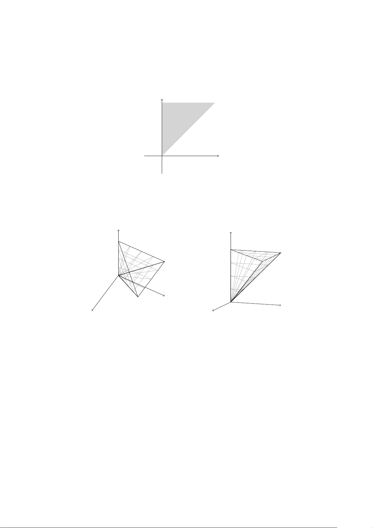
INTR ODUCING PIXELA TION WITH APPLICA TIONS J. DAISIE R OCK Abstract. Motiv ated by the desire for a new kind of approximation, we deﬁne a type of localization called pixelation . W e present how pixelation manifests in representation theory and in the study of sites and sheav es. A path category is constructed from a set, a collection of “paths” into the set, and an equiv alence relation on the paths. A screen is a partition of the set that resp ects the paths and equiv alence relation. F or a commutativ e ring, we also enrich the path category o ver its mo dules (=linearize the category with resp ect to the ring) and quotient by an ideal generated by paths (possibly 0). The pixelation is the lo calization of a path category , or the enriched quotient, with resp ect to a screen. The lo calization has useful prop erties and serves as an approximation of the original category . As applications, we use pixelations to provide a new point of view of the Zariski topology of lo calized ring sp ectra, pro vide a parallel story to a ringed space and shea ves of mo dules, and construct a categorical generalization of higher Auslander algebras of type A . Contents In tro duction 1 1. P aths and screens 5 2. P ath Categories 14 3. Represen tations 28 4. Sites and pathed sites 34 5. Higher Auslander C ategories 44 References 55 Intr oduction Con text and Motiv ation. There is an increasing interest in studying represen- tations of categories with inﬁnitely-many ob jects. That is, studying the category of functors C → K where C is a small category with inﬁnitely-man y ob jects and K is some well-understoo d ab elian category . W ork typically b egins by studying the case where C is either a line (t yp e A , though not necessarily totally-ordered) or a circle (type ˜ A , though not necessarily cyclicly ordered). Often, C is replaced b y some additiv e category A so that A and K are b oth enric hed ov er k -mo dules, for some commutativ e ring k , and the functors are re- placed with additive functors enriched o v er k -mo dules as w ell. In the language of represen tation theory: we sa y A , K , and the functors A → K are k -linear. In top ological data analysis, a p ersistence mo dule is usually a functor from a small category in to the category of ﬁnite-dimensional k -v ector spaces, for some Date : 26 March 2026. 2020 Mathematics Subje ct Classiﬁc ation. Primary: 18E35, 18A25, 18F20. Secondary: 18G15, 16G20, 16G99. Key wor ds and phr ases. pixelation, approximation, localization, representation theory , functor category , ring sp ectra, ringed space, sheaf of mo dules, higher Auslander algebra, higher homolog- ical algebra, quiver representations. 1 2 J. DAISIE ROCK ﬁeld k . In this case the persistence mo dules decomp ose uniquely (up to isomor- phism) into indecomp osable summands, each of whic h has a lo cal endomorphism ring [ GR97 , BCB20 ]. Recent work has b egun in decomp osing inﬁnite p ersistence mo dules of type A ov er other t yp es of rings, such as PIDs [ LHP25 ]. One may also consider m ultiparameter p ersistence mo dules, which can b e interpreted as represen- tations as R n . Here, complete decomposition/structure theorems are not possible but progress is made to understand persistence modules in other wa ys using in v ari- an ts [ ABH24 ]. A structure similar to p ersistence mo dules app ears as F o ck space represen tations of contin uum quantum groups of t yp es A and ˜ A [ SS21 ]. Finitely-indexed p ersis- tence mo dules can also be considered as representations of quiv ers. An inﬁnite generalization of quiv er representations was in troduced in [ BvR13 ]. A further gen- eralization and partial structure theorem and classiﬁcations app ears in [ PR Y24 ]. In all of these cases, the category C of interest has a notion of paths that are not just morphisms but also in a sense top ological or geometric. One w a y to b etter understand representations in these cases is to consider ap- pro ximations. In [ PR Y24 ] a tec hnique w as used to reduce represen tations to smaller, understandable parts. The technique splits representations in to noise and noise-free pieces. One can view this as an appro ximation b y deciding what kind of noise is allo wed in the representations. The precursor to this technique was used in [ HR24 ] and this tec hnique is the precursor to pixelation in the present pap er. A homo- logical t yp e of approximation was used in [ BBH22 ] on multiparameter p ersistence mo dules. In the presen t pap er, we think about appro ximation via lo calization. While the applications are heavily tied to represen tation theory , with the exception of some results on sites and ring sp ectra in Section 4.2 , the main techniques and re- sults in the present pap er are primarily categorical in nature. In the categorical sense lo calization as approximation is philosophically straigh tforw ard: one groups ob jects together based on some parameters, including morphisms, and this is an appro ximation of the original category . W e can think of lo calizations of rings as appro ximations as well, by lo oking at ho w the corresp onding ring sp ectra are re- lated. W e lo ok at the categories of open sets and inclusions and see if one is related to the other by some kind of categorical lo calization pro cess. Our approach to approximation dra ws inspiration from a real world pro cess: digital photography . One takes a photo of what (feels lik e) inﬁnitely-many tiny atoms and obtains a photo with a ﬁnite num ber of pixels. In its infancy , digital photos w ere very clearly (p o or) approximations of what w e see in the real w orld. In 2026, we can pro duce digital photos with more than enough pixels to accurately appro ximate what we see. How ev er, ev en at the b eginning, we only needed a few pixels to kno w if the coﬀee p ot was full. 1 Organization and con tributions. Here we give an ov erview of the pap er and highligh t what the author considers to be the main results: Theorems A , B , C , and D . How ever, given the extremely v aried interests of those who use representation theory , the reader may ﬁnd other results to b e the “highlight”. Path c ate gories and pixelation. In Section 1 w e deﬁne triples ( X , Γ / ∼ ) , where X is a set, Γ acts lik e a set of paths in X , an ∼ is an equiv alence relation on Γ (Deﬁnitions 1.1 and 1.2 ). Throughout the pap er w e use the running examples of R and R n , starting with Example 1.5 . Inspired by our approach to appro ximation, we 1 The ﬁrst digital camera had a resolution of 128x128 pixels and was used to chec k the coﬀee pot in a break ro om at the Universit y of Cambridge. The client softw are was written by Quentin Staﬀord-F raser and the server softw are was written by Paul Jardetzky . INTRODUCING PIXELA TION WITH APPLICA TIONS 3 deﬁne a sp ecial type of partition on the set X , called a scr e en , that “plays nice” with Γ and ∼ (Deﬁnition 1.12 ). The elemen ts of a screen are called pixels . W e prov e that the set P of screens on a triple ( X , Γ / ∼ ) has at least one maximal elemen t (Prop osition 1.16 ) and show that triples and screens behav e well with resp ect to pro ducts (Prop ositions 1.10 and 1.25 ). In Section 2 w e study path categories (Deﬁnition 2.1 ). A p ath c ate gory C is constructed from a triple ( X , Γ / ∼ ) . The ob jects are p oin ts in X and morphisms are equiv alence classes [ γ ] of paths in Γ using the relation ∼ . The category P C at is the sub category of C at (the category of small categories) whose ob jects are path categories and whose morphisms are functors betw een path categories. W e also deﬁne a k -linear v ersion C , for a commutativ e ring k . A p ath-b ase d ide al I in C is an ideal that behav es well with respect to paths (Deﬁnition 2.8 ). The quotient C / I is written A and is the ob ject of study in the k -linear case. W e show that, giv en a screen P of ( X , Γ / ∼ ) , there is an induced class Σ P of mor- phisms in C that admits a calculus of fractions (Prop osition 2.17 ). The lo calization C P = C [Σ − 1 P ] is called a pixelation (Deﬁnition 2.20 ). W e note that pixelation de- p ends on the choice of triple and ask when is the lo calization of a path category is a pixelation with respect to a triple and a screen (Remark 2.23 and Question 2.24 ). In C we expand I to an ideal I P compatible with P and tak e a further quotien t A P = C / I P . Notice A P is also a quotient of A . In this case w e also hav e an induced class of morphisms Σ P in A P that admits a calculus of fractions (Prop osition 2.19 ). W e also call the lo calization A P = A P [Σ − 1 P ] a pi xelation. Giv en a screen P of ( X , Γ / ∼ ) , w e construct categories Q ( C , P ) and Q ( A , P ) equiv alent to C P and A P , resp ectiv ely (Theorem 2.37 ). Eac h of Q ( C, P ) and Q ( A , P ) are its own respective skeleton and are constructed from quivers. W e essen tially prov e that pixelation yields a new path category , in the non- k - linear case. Theorem A (Theorem 2.43 ) . L et C b e the p ath c ate gory c onstructe d fr om ( X , Γ / ∼ ) and let P b e a scr e en of ( X , Γ / ∼ ) . Then Q ( C, P ) is isomorphic to a p ath c ate gory and so C P is e quivalent to a p ath c ate gory. W e introduce ﬁnitary reﬁnements (Deﬁnition 2.44 ). If P and P ′ are screens, and P ′ reﬁnes P , then w e ha v e induced functors C P ′ → C P and A P ′ → A P , since pixelation is a lo calization. This yields induced functors Q ( C, P ′ ) → Q ( C, P ) and Q ( A , P ′ ) → Q ( A , P ) , resp ectively . If P ′ is a ﬁnitary reﬁnement of P , then we also ha ve a functor Init : Q ( C , P ) → Q ( C , P ′ ) (Prop osition 2.45 ). R epr esentations. In Section 3 w e study representations of path categories with v al- ues in a k -linear abelian category K . A r epr esentation of A with values in K is a functor M : A → K (Deﬁnition 3.1 ). The category of such representations is denoted Rep K ( A ) . W e discuss the k -linear v ersion here but nearly all of the state- men ts hold for representations of C . A represen tation M is pixelate d if there is a compatible screen P and we say the screen P pixelates M (Deﬁnition 3.4 ). W e sho w that every pixelated representation M comes from a representation of some Q ( A , P ) , where P pixelates M (Theorem 3.7 ). Let L ⊆ P b e a set of screens of ( X , Γ / ∼ ) such that, for any ﬁnite collection { P i } n i =1 ⊂ L , there exists a P ∈ L that reﬁnes each P i . The category Rep L K ( A ) is the full sub category of Rep K ( A ) such that if M is a representaiton in Rep L K ( A ) then there is a screen P ∈ L such that P pixelates M . 4 J. DAISIE ROCK Theorem B (Theorem 3.10 and Corollary 3.14 ) . The c ate gory Rep L K ( A ) is a wide sub c ate gory of Rep K ( A ) . That is, Rep L K ( A ) is ab elian and the emb e dding Rep L K ( A ) → Rep K ( A ) is exact. Mor e over, any exact structur e E on Rep K ( A ) r estricts to an exact structur e on Rep L K ( A ) . Sites and she aves. In section 4 w e study how pixelation interacts with sites and shea ves. W e show that if a path category C is a site then so is Q ( C, P ) and the induced functor C → Q ( C , P ) is contin uous (Theorem 4.8 ). W e also show that a distributiv e lattice can b e interpreted as a path category . When C is a sublattice of a larger lattice L , w e deﬁne a screen P Y for eac h Y ∈ L (Deﬁnition 4.9 ) and prov e C P Y is isomorphic to a sublattice of C (Theorem 4.12 ). The theorem may b e con textualized as follo ws, where we write T op( X ) to b e the category whose ob jects are op en sets of X and whose morphisms are the inclusion maps of the open sets. Theorem C (Corollary 4.13 ) . In incr e asing sp e ciﬁcity: (1) L et X b e a top olo gic al sp ac e and Y a subset with the subsp ac e top olo gy. Then T op( Y ) is c anonic al ly isomorphic to Q (T op( X ) , P Y ) . (2) L et R b e a c ommutative ring and p b e a prime ide al in R . L et Y ( p ) = { q ∈ Sp ec( R ) | q ⊂ p } . Then T op(Sp ec( R p )) is c anonic al ly isomorphic to Q (T op(Sp ec( R )) , P Y ( p ) ) . That is, we may view T op(Spec( R p )) as a pixelation of T op(Sp ec( R )) . W e also present a parallel story to ringed sites ( X, O X ) and O X -mo dules. W e deﬁne p athe d sites ( E , O E ) to be a site E with a sheaf of path categories O E . As the “standard” example, w e show that if P admits a sub category P that is a site (Deﬁnition 4.15 ), then there is a sheaf O P on P where a screen P is sent to Q ( C, P ) and the m orphisms are the Init functors from Section 2 . The parallel to an O X -mo dule is an O E -r epr esentation (Deﬁnition 4.20 ). Similar requiremen ts for an O X -mo dule are axiomized in a w a y that works with represen- tations in our setting (functors) without running into trouble with foundations. W e pro vide a “classical” example of an O E -represen tation (Example 4.21 ) and an exam- ple of an O P -represen tation, where P is the set of screens of R n (Example 4.23 ). Higher Auslander c ate gories. In Section 5 we present an application of pixelation to higher homological algebra. Sp eciﬁcally , we lo ok at higher Auslander categories, as- sume k is a ﬁeld, and K = k - vec , the category of ﬁnite-dimensional k -vector spaces. W e pro vide a con tin uous version of the story in [ OT12 ], using some p ersp ectiv e from [ JKPK19 ]. W e deﬁne the higher Auslander c ate gory of typ e A , denoted A ( n ) R , for any n ≥ 1 (De ﬁnition 5.10 ). In this setting we consider ﬁnitely-presented mo dules, which coincide with a par- ticular rep A (n) ( A ( n ) R ) , as deﬁned in Section 3.2 , with a speciﬁed A ( n ) ⊂ P . The category rep pwf ( A ( n ) R ) is the category ob jects are functors into ﬁnite-dimensional k -v ector spaces, called p ointwise ﬁnite-dimensional , and rep A (n) ( A ( n ) R ) is a sub cate- gory of rep pwf ( A ( n ) R ) . F or each n ≥ 1 w e deﬁne a sub category M ( n ) of rep A (n) ( A ( n ) R ) and show add M ( n ) is ( n − 1) -cluster tilting in rep A (n) ( A ( n ) R ) (Prop osition 5.20 ). Since we are w orking in the contin uum, w e ha ve to take a quotient of M ( n ) , denoted M ( n ) (Deﬁnition 5.21 ). Then we ha ve the follo wing result. Theorem D (Theorem 5.22 ) . L et n ≥ 1 in N . Then M ( n ) op ∼ = A ( n +1) R . Con v en tions. W e use k for an asso ciativ e, comm utative ring with unit and use k - Mo d for the category of k -mo dules. F or the category theorists: when w e sa y “ k -linear” we mean “enriched ov er k -mo dules”, for our commutativ e ring k . When INTRODUCING PIXELA TION WITH APPLICA TIONS 5 w e sa y “a k -linear functor” w e mean “an additive k -linear functor.” When k is a ﬁeld, the categories k - V ec and k - v ec are the category of all k -v ector spaces and the category of ﬁnite-dimensional k -v ector spaces, resp ectively . Finally , the author is of the opinion that 0 ∈ N . F uture directions. There are a num b er of wa ys to pro ceed with pixelation. The ﬁrst consideration is multi-parameter p ersistence mo dules. In [ BBH22 , BBH23 , ABH24 , BDL25 ], work is b eing done to understand inv ariants of p ersistence mo d- ules since, in full generality , there is no hop e for a complete structure theorem. The pro cess of pixelation and the results in Section 3 are directly connected to homolog- ical approximation and using these kinds appro ximations to understand in v ariants. Ho wev er, proofs and careful computations need to be done in order to prop erly establish suc h a connection. There is also the in teresting case of Möbius homology (see [ PS26 ]). It w ould be interesting to see if the results in Sections 3 and 4 can b e merged together in this particular con text and, if so, in what wa y . A dditionally , the story for pathed sites has barely b egun. Is the category of O E -represen tations ab elian? If not, why? What mo diﬁcations to the deﬁnitions can be made so that the category of O E -represen tations is abelian. Assuming the category of O E -represen tations is ab elian, what is the parallel construction to (quasi-)coheren t sheav es in the pathed site story? What requiremen ts are needed on E or the path categories in O E to tell this story? What can we learn in the w ord of algebraic geometry by taking this p erspective? Finally , the deﬁnition of path categories in the presen t pap er do es not allow for “parallel paths,” i.e. paths whose images are the same but count as separate. F or example the arro ws of the Kronic k er quiver are not p ermitted in the deﬁnition of a path category in the presen t pap er: 1 ⇒ 2 . It should b e p ossible to mo dify or augmen t the presented constructions to allow such parallel paths but the present pap er is already 55 pages long. A c kno wledgemen ts. The author would lik e to thank Karin M. Jacobsen for in- spiring discussions early on regarding higher Auslander algebras. The author w ould also like to thank Eric J. Hanson, Charles Paquette, and Emine Yıldırım whose pre- vious collab orations with the author informed some of the p erspectives taken in the presen t pap er. F unding. The author is supp orted by FW O grant 1298325N. W ork on this pro ject b egan while the author was supp orted by BOF grant 01P12621 from Universiteit Gen t. The author was also partially supported b y the FWO gran ts G0F5921N (Odysseus) and G023721N, and by the KU Leuv en grant iBOF/23/064. 1. P a ths and screens In this section we introduce the tw o main structures that we will use in the presen t paper. In Section 1.1 we introduce a coherent triple of a set X , a collection of “paths” γ : [0 , 1] → X , and an e quiv alence relation ∼ on the paths. In Section 1.2 w e introduce a sp ecial t ype of partition, called a scr e en . W e will extensively use the prop erties of these triples and screens for the rest of the pap er. 1.1. P aths. W e b egin b y deﬁning a coheren t set of paths Γ (Deﬁnition 1.1 ) and a useful equiv alence relation ∼ on the paths (Deﬁnition 1.2 ). Let X be a nonempty set. Ev en though X need not come from a top ological space, we refer to a function [0 , 1] → X as a p ath . W e comp ose paths similar to those in a top ological setting. Giv en γ : [0 , 1] → X and γ ′ : [0 , 1] → X suc h that 6 J. DAISIE ROCK γ (1) = γ ′ (0) , we create a new path γ · γ ′ : [0 , 1] → X given b y γ · γ ′ ( t ) = ( γ (2 t ) 0 ≤ t ≤ 1 2 γ ′ (2( t − 1 2 )) 1 2 ≤ t ≤ 1 . Deﬁnition 1.1 ( Γ ) . Let X b e a nonem tpy set and let Γ b e a subset of paths in X that satisﬁes the following. (1) Close d under c omp osition : If γ , γ ′ ∈ Γ and γ (1) = γ ′ (0) then γ · γ ′ ∈ Γ . (2) Close d under subp aths : F or each γ ∈ Γ and eac h (weakly) order preserving map φ : [0 , 1] → [0 , 1] such that φ sends interv als to in terv als, the path γ φ is in Γ , where γ φ is the functional comp osition. (3) Close d under c onstant p aths : F or each x ∈ X , the constant path at x is in Γ . That is, for each x ∈ X there is a γ ∈ Γ such that for all t ∈ [0 , 1] we ha ve γ ( t ) = x . W e note that we explicitly do not assume anything ab out Γ b ey ond the items in the deﬁnition. In particular, we are not assuming any ﬁniteness, discreteness, cardinalit y , partial order, cyclic order, etc. The most natural example of X and Γ is to tak e X as a top ological space and Γ as all paths in to X . Ho w ev er, this is exceedingly cumbersome. A more con v enient example is to take a manifold X with some kind of ﬂow and tak e the paths Γ that follo w the ﬂo w. An interesting example is to take X to b e a p oset with relation ≤ and insist that, for each γ ∈ Γ , we ha ve γ ( t ) ≤ γ ( s ) if and only if t ≤ s in [0 , 1] . One could also consider thread quivers from [ BvR13 , PR Y24 ]. Then, in most cases, the paths in the thread quivers are the images of the paths in Γ . Deﬁnition 1.2 ( ∼ ) . Giv en a nonempty set X and a Γ satisfying Deﬁnition 1.1 , we deﬁne an equiv alence relation ∼ on Γ satisfying the follo wing requirements. (1) A c onstant p ath is only e quivalent to itself : If γ ∼ γ ′ and γ is constant then so is γ ′ . (2) Equivalenc e classes ar e close d under r ep ar ameterization : If γ ∈ Γ and φ : [0 , 1] → [0 , 1] is a w eakly order-preserving map that sends interv als to interv als, 0 to 0, and 1 to 1, then γ ∼ γ φ . (3) Equivalenc e classes c omp ose : Given γ , γ ′ , ρ, ρ ′ ∈ Γ such that ρ · γ · ρ ′ and ρ · γ ′ · ρ ′ are in Γ , we ha v e γ ∼ γ ′ ∈ Γ if and only if ρ · γ · ρ ′ ∼ ρ · γ ′ · ρ ′ . Immediately we see that if γ ∼ γ ′ , ρ 1 ∼ ρ ′ 1 , ρ 2 ∼ ρ ′ 2 , ρ 1 (1) = ρ ′ 1 (1) = γ (0) = γ ′ (0) , and ρ 2 (0) = ρ ′ 2 (0) = γ (1) = γ ′ (1) , then ρ 1 · γ · ρ 2 ∼ ρ ′ 1 · γ ′ · ρ ′ 2 b y using Deﬁnition 1.2 ( 3 ) ab ov e. First changing ρ 1 to ρ ′ 1 , then ρ 2 to ρ ′ 2 , and ﬁnally γ to γ ′ . Giv en X , Γ , and ∼ , we write the triple as ( X , Γ / ∼ ) . Remark 1.3. In a top ological setting, our equiv alence relation ∼ is generally ﬁner than homotop y equiv alence of paths. The relation ∼ cannot b e homotopy equiv a- lence of paths if Γ con tains a path γ , with γ (0) = γ (1) and some some a ∈ [0 , 1] suc h that γ ( a )  = γ (0) , where γ is homotopy equiv alent to a constan t path. Notation 1.4 ( ∼ -equiv alence classes) . Giv en γ ∈ Γ , the set of all γ ′ ∈ Γ suc h that γ ∼ γ ′ is denoted [ γ ] . I.e., [ γ ] is the ∼ -equiv alence class of γ . The following example is the start of our running example throughout the pap er. Example 1.5 (running example) . Let X = R and let Γ b e all con tin uous functions γ : [0 , 1] → R where s ≤ t implies γ ( s ) ≤ γ ( t ) . F or the purposes of the w ord “con tinuous”, we consider [0 , 1] and R to hav e the usual top ologies. Let γ ∼ γ ′ if γ (0) = γ ′ (0) . Then it is straigh tforw ard to chec k that ( X , Γ / ∼ ) satisﬁes Deﬁni- tions 1.1 and 1.2 . INTRODUCING PIXELA TION WITH APPLICA TIONS 7 Notation 1.6 ( R ) . Ov erloading notation, if we write ab out R as if it is a triple ( X , Γ / ∼ ) , then w e mean the triple ( R , Γ / ∼ ) in Example 1.5 . Our triples ( X , Γ / ∼ ) form a category in a natural wa y . Deﬁnition 1.7 ( X ) . W e deﬁne the category X to b e the category whose ob jects are triples ( X , Γ / ∼ ) satisfying Deﬁnitions 1.1 and 1.2 and whose morphisms are deﬁned as follo ws. Let ( X 1 , Γ 1 / ∼ 1 ) and ( X 2 , Γ 2 / ∼ 2 ) satisfy Deﬁnitions 1.1 and 1.2 and let f : X 1 → X 2 b e a function of sets. W e say f : ( X 1 , Γ 1 / ∼ 1 ) → ( X 2 , Γ 2 / ∼ 2 ) is a morphism in X if the following conditions are satisﬁed. (1) If γ ∈ Γ 1 then f ◦ γ ∈ Γ 2 . (2) If γ , γ ′ ∈ Γ 1 and γ ∼ 1 γ ′ then f ◦ γ ∼ 2 f ◦ γ ′ . Prop osition 1.8. The X in Deﬁnition 1.7 is a c ate gory. Pr o of. Suppose f : ( X 1 , Γ 1 / ∼ 1 ) → ( X 2 , Γ 2 / ∼ 2 ) and g : ( X 2 , Γ 2 / ∼ 2 ) → ( X 3 , Γ 3 / ∼ 3 ) are morphisms. W e see that if γ ∈ Γ 1 then f ◦ γ ∈ Γ 2 and so g ◦ ( f ◦ γ ) ∈ Γ 3 . Moreo ver, if γ ∼ 1 γ ′ , for γ , γ ′ ∈ Γ 1 , then we know f ◦ γ ∼ 2 f ◦ γ ′ and so g ◦ ( f ◦ γ ) ∼ 3 g ◦ ( f ◦ γ ′ ) . Th us, g ◦ f is also a morphism. T rivially , the identit y map on an y ( X , Γ / ∼ ) is a morphism. And, since func- tions b et w een sets comp ose associatively , we see that morphisms also compose asso ciativ ely . Finally , recall that each ( X , Γ / ∼ ) is a collection of sets and relations. Therefore, there is a category of triples ( X , Γ / ∼ ) satisfying Deﬁnitions 1.1 and 1.2 with the morphisms we ha v e just describ ed. □ The terminal ob jects in X are the ob jects in the the isomorphism class of ( {∗} , { γ } / ∼ ) , where γ is the constant path at ∗ . The equiv alence relation is trivial. W e no w describ e pro ducts in X . Deﬁnition 1.9 (pro duct of triples) . Let { ( X i , Γ i / ∼ i ) } i ∈ I b e a set-sized collection of triples in X . W e deﬁne a new triple ( X , Γ / ∼ ) in X as follo ws. • Deﬁne X = Q i ∈ I X i . • W e sa y a function γ : [0 , 1] → X is in Γ if π i ◦ γ ∈ Γ i , for each i ∈ I . • F or a pair γ , γ ′ ∈ Γ , w e say γ ∼ γ ′ if π i ◦ γ ∼ i π i ◦ γ ′ for each i ∈ I . W e also write ( X , Γ / ∼ ) as Q i ∈ I ( X i , Γ i / ∼ i ) . The following prop osition says that we ha v e all pro ducts in X . Prop osition 1.10. L et { ( X i , Γ i / ∼ i ) } i ∈ I b e a set-size d c ol le ction of triples in X . Then ( X , Γ / ∼ ) = Q i ∈ I ( X i , Γ i / ∼ i ) is the pr o duct in X . Pr o of. First we show Q i ∈ I ( X i , Γ i / ∼ i ) is a triple in X and then we show that it is indeed the product in X . It is straightforw ard to chec k that Γ satisﬁes Deﬁnition 1.1 , so we fo cus on showing that Deﬁnition 1.2 is satisﬁed. Deﬁnition 1.2 ( 1 ) . Supp ose γ , γ ′ ∈ Γ , γ ∼ γ ′ , and γ is constant. Then, for eac h 1 ≤ i ≤ n , we ha v e π i γ ∼ i π i γ ′ and each π i γ is constant. Then π i γ ′ is constant for eac h i ∈ I and so γ ′ is constant also. Deﬁnition 1.2 ( 2 ) . Let γ ∈ Γ and let φ : [0 , 1] → [0 , 1] b e a weakly order- preserving map that sends in terv als to interv als, 0 to 0, and 1 to 1. F or each i ∈ I , w e hav e π i γ φ ∼ i π i γ . Then we hav e γ φ ∼ γ . 8 J. DAISIE ROCK Deﬁnition 1.2 ( 3 ) . Let γ , γ ′ , ρ, ρ ′ ∈ Γ suc h that ρ · γ · ρ ′ and ρ · γ ′ · ρ ′ are also in Γ . Then w e hav e γ ∼ γ ′ ⇔ π i γ ∼ i π i γ ′ , ∀ i ∈ I ⇔ π i ρ · π i γ · π i ρ ′ ∼ i π i ρ · π i γ ′ · π i ρ ′ , ∀ i ∈ I ⇔ π i ( ρ · γ · ρ ′ ) ∼ i π i ( ρ · γ ′ · ρ ′ ) , ∀ i ∈ I ⇔ ρ · γ · ρ ′ ∼ ρ · γ ′ · ρ ′ . No w we sho w that ( X , Γ / ∼ ) = Q i ∈ I ( X i , Γ i / ∼ i ) is the pro duct in X . Notice that, b y construction, eac h π i is a morphism ( X , Γ / ∼ ) → ( X i , Γ i / ∼ i ) . Let ( Y , ∆ / ≈ ) b e a triple in X and, for eac h i ∈ I , let f i : ( Y , ∆ / ≈ ) → ( X i , Γ i / ∼ i ) b e a morphism. Deﬁne f : Y → X by y 7→ ( f 1 ( y ) , . . . , f n ( y )) . W e see immediately that, as functions of sets, π i ◦ f = f i , for each i ∈ I . It remains to show that f is a morphism in X . Let δ ∈ ∆ . Then f ( δ ) = ( f 1 ( δ ) , . . . , f n ( δ )) . W e kno w that each f i ( δ ) ∈ Γ i , for i ∈ I . Thus, by deﬁnition, f ( δ ) ∈ Γ . Supp ose δ ≈ δ ′ . Then, for each i ∈ I , f i ◦ δ ∼ i f i ◦ δ ′ . Th us, by deﬁnition, f ◦ δ ∼ f ◦ δ ′ . Therefore f is a morphism and so ( X , Γ / ∼ ) is the pro duct in X . □ Example 1.11 (running example) . Let n ∈ N > 1 and let ( X i , Γ i / ∼ i ) = R (from Example 1.5 ), for each 1 ≤ i ≤ n . W e will often denote b y simply R n the product Q n i =1 R = Q n i =1 ( X i , Γ i / ∼ i ) in X . 1.2. Screens. In this section we consider partitions of X that satisfy some condi- tions, called screens (Deﬁnition 1.12 ), and prov e some fundamental prop erties w e will need later. W e use P for partitions and X , Y , Z ... for the elemen ts of the partition. I.e., X ∈ P and X ⊆ X . Deﬁnition 1.12 (screen) . Giv en a triple ( X , Γ / ∼ ) in X , a partition P of X is a scr e en if the following are satisﬁed. (1) Elements of P ar e ∼ -thin : Consider γ , γ ′ ∈ Γ such that im( γ ) ⊂ X ∈ P , γ (0) = γ ′ (0) , γ (1) = γ ′ (1) . Then γ ∼ γ ′ if and only if im( γ ′ ) ⊂ X . (2) Elements of P ar e Γ -c onne cte d : F or any x, y ∈ X ∈ P there is a ﬁnite w alk γ 0 · γ − 1 1 · γ 2 · · · γ − 1 2 n − 1 · γ 2 n , with γ 0 (0) = x , γ 2 n (1) = y , ∀ i ( γ i ∈ Γ) , and ∀ i (im( γ i ) ⊂ X ) , where γ − 1 means to do the path backw ards and any γ i ma y b e the constant path. (3) P has an Or e c ondition : Consider the square of paths in X : ρ ρ ′ γ γ ′ If ρ, γ ∈ Γ , and im( ρ ) ⊂ X ∈ P , then there exists ρ ′ , γ ′ ∈ Γ suc h that im( ρ ′ ) ⊂ Y ∈ P and γ · ρ ′ ∼ ρ · γ ′ . Similarly , if ρ ′ , γ ′ ∈ Γ and im( ρ ′ ) ⊂ Y ∈ P then there exists ρ, γ ∈ Γ suc h that im( ρ ) ⊂ X ∈ P and ρ ′ · γ ∼ γ ′ · ρ . (4) P is discr ete : F or any path γ ∈ Γ , there is a ﬁnite partition { I i } n i =1 of [0 , 1] and a corresponding ﬁnite list ( X 1 , . . . , X n ) of pixels in P satisfying the follo wing conditions. Each I i is a subinterv al and if t ∈ I i then γ ( t ) ∈ X i . W e allo w the p ossibility that X i = X j only if | j − i | > 1 . INTRODUCING PIXELA TION WITH APPLICA TIONS 9 (5) P maintains e quivalenc es : Assume γ , γ ′ ∈ Γ with the same partitions { I i } n i =1 = { I ′ i } n i =1 and lists ( X 1 , . . . , X n ) = ( X ′ 1 , . . . , X ′ n ) , from ( 4 ). As- sume also that γ (0) = γ ′ (0) , γ (1) = γ ′ (1) , and if t ∈ I i = I ′ i then γ ( t ) , γ ′ ( t ) ∈ X i = X ′ i . Then γ ∼ γ ′ . If P is a screen w e call its elements pixels . Example 1.13 (running example) . Let R b e the triple from Example 1.5 and let P = { [ i, i + 1) | i ∈ Z } . Then P is a screen of R . In fact, a short consideration of Deﬁnition 1.12 reveals that, for an y screen P of R , every pixel X ∈ P is an interv al. The discreteness requiremen t means that screens of R are those partitions of R (as a set) where, for any arbitrary b ounded in terv al I ⊂ R , there are ﬁnitely-many pixels X ∈ P suc h that I ∩ X  = ∅ . The “one dimensional” v ersion of a screen, like the one in Example 1.13 , comes from the study of thread quiv ers and can b e found in [ PR Y24 , Deﬁnition 2.6]. F or the rest of this section, w e ﬁx a triple ( X , Γ / ∼ ) in X . The following lemma is a useful reduction of Deﬁnition 1.12 ( 2 ) that w e will use throughout the paper. Lemma 1.14. L et P b e a scr e en of ( X , Γ / ∼ ) and let X ∈ P . F or any x, y ∈ X , ther e is a walk of 2 p aths fr om x to y in X . Pr o of. By Deﬁnition 1.12 ( 2 ), let γ 0 · γ − 1 1 · γ 2 · · · γ − 1 2 n − 1 · γ 2 n b e ﬁnite walk where γ 0 (0) = x , γ 2 n (1) = y , and im( γ i ) ⊂ X for each 0 ≤ i ≤ 2 n . Consider γ 1 and γ 2 . W e know γ 1 (0) = γ 2 (0) and so w e can use Deﬁnition 1.12 ( 3 ) to obtain tw o new paths γ ′ 1 and γ ′ 2 , where im( γ ′ 1 ) ⊂ X . This gives us the follo wing picture in X : γ 1 γ ′ 2 γ 2 γ ′ 1 And, w e kno w γ 2 · γ ′ 1 ∼ γ 1 · γ ′ 2 . So, im( γ 2 · γ ′ 1 ) ⊂ X . By Deﬁnition 1.12 ( 1 ), w e m ust ha ve im( γ 1 · γ ′ 2 ) ⊂ X . Now w e hav e the following paths in X : . . . γ 0 γ 1 γ 2 γ 3 γ ′ 2 γ ′ 1 If w e replace γ 0 · ( γ 1 ) − 1 · γ 2 · ( γ − 3) − 1 with ( γ 0 · γ ′ 2 ) · ( γ 3 · γ ′ 1 ) − 1 , w e ha v e shortened our walk by t w o paths. W e can rep eat this pro cess to get a walk γ ′′ 0 ( γ ′′ 1 ) − 1 from x to y . Similarly , we may construct a walk γ ′′ 0 ( γ ′′ 1 ) − 1 γ ′′ 2 from x to y such that γ ′′ 0 is a constan t path, whic h is eﬀectiv ely a w alk of tw o paths. □ Deﬁnition 1.15 ( P ) . Denote by P the p oset of all screens on ( X , Γ / ∼ ) . W e say P ≤ P ′ if P reﬁ nes P ′ . Prop osition 1.16. If P is nonempty then it has at le ast one maximal element. Pr o of. W e will use the Kuratowski—Zorn lemma (commonly kno wn as Zorn’s lemma). Let T ⊂ P b e a chain. Deﬁne morphisms P → P ′ whenev er P ≤ P ′ in T b y X 7→ X ′ if X ⊂ X ′ . In the category of sets, let P T b e the colimit of T , where we 10 J. DAISIE ROCK iden tity the elemen ts X ∈ P T with [ X ∈ P ∈ T , X 7→ X X . Overloading notation, we set X equal to this big union. First we show that P T is a partition. Let x ∈ X . F or each P ∈ T , there exists a unique X ∈ P suc h that x ∈ X . Then, there is some X ∈ P T suc h that X ⊆ X and so x ∈ X . Supp ose x ∈ X ∩ Y , for X , Y ∈ P T . Then for an y P ∈ T there are X , Y ∈ P such that x ∈ X , x ∈ Y , X ⊆ X , and Y ⊆ Y . Then x ∈ X ∩ Y so X = Y whic h implies X = Y . Therefore, P T is a partition of X . No w we will sho w that P T is a screen. W e start with Deﬁnition 1.12 ( 4 ). Let γ ∈ Γ and let P ∈ T . W e kno w there is a ﬁnite partition { I i } n i =1 of [0 , 1] and list X 1 , . . . , X n of pixels in P (p ossibly with rep etition), such that, on each I i , im( γ | I i ) is contained in the pixel X i . F or each 1 ≤ i ≤ n , let X i b e the pixel in P T that con tains X i . Then w e see immediately that P T is also discrete. T ric k: W e will reuse the follo wing trick. W e now show that if im( γ ) ⊂ X ∈ P T , there exists P ∈ T such that im( γ ) ⊂ X ∈ P where X ⊆ X ∈ P T . Let X ∈ P T and let γ ∈ Γ b e some path such that im( γ ) ⊂ X . Let P ′′ ∈ T and notice that, since P ′′ is discrete, w e ha v e the ﬁnite list of pixels X ′ 1 , . . . , X ′ n ′′ and corresponding partition { I ′ i } n i =1 of [0 , 1] from the previous paragraph. Since X ′ i ⊆ X for each 1 ≤ i ≤ n , there is some P ∈ T suc h that S n i =1 X i ⊆ X ∈ P ′ . Then im( γ ) ⊂ X ∈ P and X ⊆ X . No w we show Deﬁnition 1.12 ( 1 ). Let γ , γ ′ ∈ Γ and X ∈ P T suc h that im( γ ) ⊂ X , γ (0) = γ ′ (0) , and γ (1) = γ ′ (1) . By our trick there is a partition P ∈ T and pixel X ∈ P such that im( γ ) ⊂ X . Then, since P is a scree n, γ ∼ γ ′ if and only if im( γ ′ ) ⊂ X . Th us, if γ ∼ γ ′ then im( γ ′ ) ⊂ X . If im( γ ′ ) ⊂ X , then by our trick there is some X ′ ∈ P ′ ∈ T such that im( γ ′ ) ⊂ X ′ . Either P ≤ P ′ or P ′ ≤ P . Let P ′′ b e the larger of the t w o and X ′′ the pixel corresp onding to X ∈ P if P is larger or X ′ ∈ P ′ if P ′ is larger. Then im( γ ) ∪ im( γ ′ ) ⊂ X ′′ and, since P ′′ is a screen, w e kno w γ ∼ γ ′ . No w we show Deﬁnition 1.12 ( 3 ). Let ρ, γ ∈ Γ such that ρ (0) = γ (0) and im( ρ ) ⊂ X ∈ P T . W e only show this version as the other is similar. Then b y our trick there is some X ∈ P ∈ T suc h that im( ρ ) ⊂ X . Then, since P is a screen, there exist paths γ ′ , ρ ′ where γ · ρ ′ ∼ ρ · γ ′ and im( ρ ′ ) ⊂ Y ∈ P . Then there is some Y ∈ P T suc h that Y ⊆ Y . No w we show Deﬁnition 1.12 ( 2 ). Let x, y ∈ X ∈ P T . Let P ′ ∈ T . Then x ∈ X ′ and y ∈ Y ′ , for X ′ , Y ′ ∈ P ′ . Since X ′ ∪ Y ′ ⊂ X , there is some P ∈ T such that X ∪ Y ′ ⊆ X ∈ P . Then x, y ∈ X so there is a ﬁnite walk in X ⊆ X from x to y . Finally , we sho w Deﬁnition 1.12 ( 5 ). Let γ , γ ′ ∈ Γ . Assume there is a partition { I i } n i =1 of [0 , 1] where eac h I i is an in terv al and if t ∈ I i then γ ( t ) , γ ′ ( t ) ∈ X i . Cho ose P ∈ T . F or each 1 ≤ i ≤ n we hav e a partition { J ij } m i j =1 of I i suc h that eac h J ij is an interv al and γ ( t ) ∈ X ij if t ∈ J ij . W e ha ve a similar partition { J ′ ij } m ′ i j =1 for γ ′ . F or each 1 ≤ i ≤ n , we hav e ( S m i j =1 X ij ) ∪ ( S m ′ i j =1 X ′ ij ) ⊂ X i . Th us, there is some P i ∈ T with X i suc h that X ij ⊂ X i and X ′ ij ′ ⊂ X i for eac h 1 ≤ j ≤ m i and 1 ≤ j ′ ≤ m ′ i . Since T is a c hain, one of the P a is maximal in { P i } n i =1 . Thus, if t ∈ I i then γ ( t ) , γ ′ ( t ) ∈ X i ⊂ X i . Since P a is a screen we know γ ∼ γ ′ , satisfying Deﬁnition 1.12 ( 5 ). This completes the pro of. W e hav e now shown that P T is a screen. □ In the present pap er, for an y triple ( X , Γ / ∼ ) in X that we consider, w e will assume P  = ∅ . INTRODUCING PIXELA TION WITH APPLICA TIONS 11 X 1 X 2 X ′ ˜ ρ ˜ γ ρ 3 ρ 4 γ ′ γ ρ 1 ρ 2 Figure 1.1. Sc hematic for the pro of of Lemma 1.18 . Remark 1.17. Deﬁnition 1.12 ( 1 ) implies that if γ (0) = γ (1) and γ is not a constant path, then there exists pixels X  = Y ∈ P with γ ( a ) ∈ X and γ ( b ) ∈ Y , for some a, b ∈ [0 , 1] . The following tec hnical lemma is helpful to pro ve Lemma 1.19 . Lemma 1.18. L et P and P ′ b e scr e ens of ( X , Γ / ∼ ) such that P r eﬁnes P ′ . Supp ose X 1 , X 2 ∈ P , X ′ ∈ P ′ and X 1 ∪ X 2 ⊂ X ′ . L et γ ∈ Γ such that γ (0) ∈ X 1 , γ (1) ∈ X 2 , and im( γ ) ⊂ X ′ . Then ther e is no γ ′ ∈ Γ such that γ ′ (0) ∈ X 2 , γ ′ (1) ∈ X 1 , and im( γ ′ ) ⊂ X ′ . Pr o of. F or contradiction, suppose suc h a γ ′ exists. The reader is encouraged to reference Figure 1.1 as a guide to the pro of. By Lemma 1.14 we hav e paths ρ 1 , ρ 2 with ρ 1 (0) = ρ 2 (0) , im( ρ 1 ) ∪ im( ρ 2 ) ⊂ X 2 , ρ 1 (1) = γ (1) , and ρ 2 (1) = γ ′ (0) . Since w e hav e γ (0) ∈ X 1 , γ (1) ∈ X 2 , and im( ρ 1 ) ⊂ X 2 , there is some ˜ γ and ˜ ρ with ˜ γ (0) = ˜ ρ (0) , ˜ ρ (1) = γ (0) , and ˜ γ (1) = ρ 1 (0) suc h that ˜ ρ · γ = ˜ γ · ρ 1 and im( ˜ ρ ) ⊂ X 1 (Deﬁnition 1.12 ( 3 )). Since ˜ γ · ρ 1 ∼ ˜ ρ · γ , we kno w im( ˜ γ ) ⊂ X ′ b y Deﬁnition 1.12 ( 1 ). Using Lemma 1.14 again, we ha ve paths ρ 3 , ρ 4 with ρ 3 (1) = ρ 4 (1) , ρ 3 (0) = ˜ γ (0) , ρ 4 (0) = γ ′ (0) , and im( ρ 3 ) ∪ im( ρ 4 ) ⊂ X 1 . Let γ ′′ = ˜ γ · ρ 2 · γ ′ · ρ 4 . No w w e ha ve im( γ ′′ ) ⊂ X ′ , im( ρ 3 ) ⊂ X ′ , γ ′′ (0) = ρ 3 (0) , and γ ′′ (1) = ρ 3 (1) . Therefore, by Deﬁnition 1.12 ( 1 ), w e hav e γ ′′ ∼ ρ 3 . But, since im( ρ 3 ) ⊂ X 1 , we must ha ve im( γ ′′ ) ⊂ X 1 also by Deﬁnition 1.12 ( 1 ). But γ ′ (0) ∈ X 2 , a contradiction. This compelets the pro of. □ No w, Lemma 1.19 is useful in multiple places, esp ecially in the pro of of Prop o- sition 2.45 . Lemma 1.19. Supp ose P and P ′ ar e scr e ens of ( X , Γ / ∼ ) and P r eﬁnes P ′ . L et X ′ ∈ P ′ and supp ose ther e exist only ﬁnitely-many pixels { X i } n i =1 such that e ach X i ⊂ X ′ . Then ther e is an initial X j in the sense that for any x i ∈ X i ther e is an x j ∈ X j and a p ath γ ∈ Γ with γ (0) = x j and γ (1) = x i . Pr o of. W e start with { X i } n i =1 ⊂ P and systematically remov e pixels X i if there is a pixel X j with a path γ ∈ Γ such that γ (0) ∈ X j and γ (1) ∈ X i . The last pixel remaining m ust b e the initial pixel among those that are subsets of X ′ , by Lemma 1.18 . First consider X 1 and X 2 . If there is a path γ ∈ Γ with γ (0) ∈ X i , γ (1) ∈ X 3 − i , and im( γ ) ⊂ X ′ , then we keep X i and remov e X 3 − i . By Lemma 1.18 , w e know there cannot b e a path from X 3 − i to X i . W e now ha ve a subset of P with n − 1 pixels. If instead there is no suc h γ , let x 1 ∈ X 1 and x 2 ∈ X 2 . Since P ′ is a screen, there is some x i ∈ X i ⊂ X ′ and paths ρ 1 , ρ 2 ∈ Γ with ρ 1 (0) = ρ 2 (0) = x i and 12 J. DAISIE ROCK im( ρ 1 ) ∪ im( ρ 2 ) ⊂ X ′ . Then we remov e b oth X 1 and X 2 . W e now hav e a subset of P with n − 2 pixels. In both cases we now hav e fewer pixels and rep eat the pro cess at most n − 1 times. The last remaining pixel is the initial pixel as desired. □ W e ha v e the follo wing equiv alence relation on paths, relative to a screen P . Deﬁnition 1.20 ( P -equiv alent paths) . W e say tw o paths γ , γ ′ ∈ Γ are P -e quivalent if there exists ρ 1 , ρ 2 , ρ 3 , ρ 4 ∈ Γ where im( ρ 1 ) ∪ im( ρ 2 ) ⊂ X ∈ P , im( ρ 3 ) ∪ im( ρ 4 ) ⊂ Y ∈ P , and ρ 1 · γ · ρ 3 ∼ ρ 2 · γ ′ · ρ 4 . Notice that if γ ∼ γ ′ (in particular if γ = γ ′ ) then γ is P -equiv alent to γ ′ , by taking ρ i to b e the iden tity for eac h i . Using Lemma 1.14 , it is straight forw ard to show that P -equiv alence is indeed an equiv alence relation. Sometimes we will consider a partition P of a set X to be the induced surjection X ↠ P in the category of sets. This p oint of view is useful to deﬁne the following op erations, for example. Deﬁnition 1.21. (meet and join of partitions) Let X ↠ P and X ↠ P ′ b e parti- tions of a set X . W e deﬁne the meet of the partitions to b e P ⊓ P ′ := { X ∩ X ′ | X ∈ P , X ′ ∈ P ′ } . W e deﬁne the join of the partitions to b e the pushout in the following diagram (in the category of sets): X / / / /     P     P ′ / / / / P ⊔ P ′ . The following prop osition follows from straigh tforward set theory . Prop osition 1.22. The op er ations ⊓ and ⊔ make the set of p artitions of a set X into a lattic e. Remark 1.23. In general, it is not true that P , P ′ ∈ P implies either P ⊓ P ′ ∈ P or P ⊔ P ′ ∈ P . This must b e done on a case-by-case basis. Ho wev er, if it is true that P , P ′ ∈ P implies P ⊓ P ′ , P ⊔ P ′ ∈ P , then P is a lattice and there is a unique maximal element in P (using Prop osition 1.16 ). Deﬁnition 1.24. (pro duct of screens) Let { ( X i , Γ i / ∼ i ) } n i =1 b e a ﬁnite collection of triples in X . F or each 1 ≤ i ≤ n , let P i b e a screen of ( X i , Γ i / ∼ i ) . The pr o duct of scr e ens , P := Q n i =1 P i is deﬁned as ( n Y i =1 X i      X i ∈ P i ) . Prop osition 1.25. L et { ( X i , Γ i / ∼ i ) } n i =1 b e a ﬁnite c ol le ction of triples in X and, for e ach 1 ≤ i ≤ n , let P i b e a scr e en of ( X i , Γ i / ∼ i ) . (1) W e have P = Q n i =1 P i is a scr e en of ( X , Γ / ∼ ) = Q n i =1 ( X i , Γ i / ∼ i ) . (2) If Q is a scr e en of ( X , Γ / ∼ ) then Q = Q n i =1 Q i wher e e ach Q i = { π i X | X ∈ Q } is a scr e en of ( X i , Γ i / ∼ i ) , for 1 ≤ i ≤ n . Pr o of. W e prov e statemen t ( 1 ) in the prop osition. F or eac h of the items in Deﬁ- nition 1.12 , we can rev erse the arguments presen ted to show statemen t ( 2 ) in the prop osition. Thus, we suppress the pro of of statement ( 2 ). It follows immediately that P is a partition of X . W e now show that P satisﬁes Deﬁnition 1.12 . INTRODUCING PIXELA TION WITH APPLICA TIONS 13 Deﬁntiion 1.12 ( 1 ) . Let γ , γ ′ ∈ Γ such that γ (0) = γ ′ (0) , γ (1) = γ ′ (1) , and im( γ ) ⊂ X ∈ P , where X = Q n i =1 X i and each X i ∈ P i . Then w e hav e γ ∼ γ ′ ⇔ π i γ ∼ i π i γ ′ , 1 ≤ i ≤ n ⇔ im( π i γ ′ ) ⊂ X i , 1 ≤ i ≤ n ⇔ π i (im γ ′ ) ⊂ X i , 1 ≤ i ≤ n ⇔ im( γ ′ ) ⊂ X . Deﬁntiion 1.12 ( 2 ) . Let x, y ∈ X ∈ P , where x = ( x 1 , . . . , x n ) and y = ( y 1 , . . . , y n ) . Then, for each 1 ≤ i ≤ n , we hav e x i , y i ∈ X i . By Lemma 1.14 , we hav e a walk ( ρ i ) − 1 γ i where ρ i (1) = x i , γ i (1) = y i , ρ i (0) = γ i (0) , and im( ρ i ) ∪ im( γ i ) ⊂ X i . Deﬁne ρ, γ : [0 , 1] ⇒ X to the unique function such that π i ρ = ρ i and π i γ = γ i , for 1 ≤ i ≤ n . Then ρ − 1 γ is a ﬁnite walk from x to y in X . Deﬁntiion 1.12 ( 3 ) . W e prov e the statement where w e start with ρ and γ as the pro of of the dual statemen t is similar. Let ρ, γ ∈ Γ such that ρ (0) = γ (0) and im( ρ ) ⊂ X . F or each 1 ≤ i ≤ n , we hav e π i ρ (0) = π i γ (0) and im( π i ρ ) ⊂ X i . Then, w e hav e ρ ′ i , γ ′ i ∈ Γ i suc h that π i γ · ρ ′ i ∼ i π i ρ · γ ′ i and im( ρ ′ i ) ⊂ Y i , for some Y i ∈ P i . Let ρ ′ , γ ′ : [0 , 1] ⇒ X b e the unique functions such that π i ρ ′ = ρ ′ i and π i γ ′ = γ ′ i . Then, γ · ρ ′ ∼ ρ · γ ′ and im( ρ ′ ) ⊂ Y = Q n i =1 Y i . Deﬁnition 1.12 ( 4 ) . Let γ ∈ Γ . F or each 1 ≤ i ≤ n , there is a partition I i = { I ij } m i j =1 of [0 , 1] where each I ij is an in terv al and im( π i γ ) | I ij is contained in X ij ∈ P i . Since w e hav e ﬁnitely man y partitions { I ij } m i j =1 , we ma y use Prop osition 1.22 and obtain I = V n i =1 I i . Since eac h I i is ﬁnite and w e hav e a ﬁnite collection, I is also a ﬁnite partition. Let T n i I ij b e nonempty , where 1 ≤ j ≤ m i for each 1 ≤ i ≤ n . Then im( π i γ ) ⊂ X ij for each I ij . So, im( γ ) ⊂ Q n i =1 X ij on T n i I ij . Deﬁnition 1.12 ( 5 ) . Let γ , γ ′ ∈ Γ and assume there is a partition { I j } m j =1 of [0 , 1] suc h that each I j is an interv al and if t ∈ I j then γ ( t ) , γ ′ ( t ) ∈ X j = Q n i =1 X ij . Then, for eac h 1 ≤ i ≤ n , and each 1 ≤ j ≤ m , if t ∈ I j then π i γ ( t ) , π i γ ′ ( t ) ∈ X ij . Th us, since each P i is a screen, π i γ ∼ i π i γ ′ . By deﬁnition, we ha ve γ ∼ γ ′ . □ Notice that we needed { ( X i , Γ i / ∼ i ) } n i =1 to b e a ﬁ nite collection near the end of the ab o v e pro of. F or those interested in screens without the dicrete requirement, one ma y drop the ﬁnite-ness requirement and instead work with { ( X α , Γ α / ∼ α ) } α and { P α } for some indexing set { α } . How ever, in the present pap er, we use the ﬁnite-nes requirement. Example 1.26 (running example) . Let R n b e the triple from Example 1.11 . Then an y screen of R n is a pro duct of screens of R as in Example 1.13 . Sp eciﬁcally , if P is a screen of R n then each pixel X ∈ P is a product of in terv als I 1 × I 2 × · · · × I n . Although we deﬁned P ⊔ P ′ to b e a pushout in the category of sets, there is an alternate construction that is useful for computations. Deﬁnition 1.27 (join complex) . Let P and P ′ b e partitions of a set X . W e now construct a CW-complex Y . Let Y 0 = P ⨿ P ′ (where w e tak e the disjoin t union in the category of sets). F or each X ∈ P and X ∈ P ′ suc h that X ∩ X ′  = ∅ , w e add a 1-cell from X to X ′ in Y 1 . The join c omplex of P ⊔ P ′ is the CW-complex Y whose 0-cells are Y 0 and whose 1-cells are Y 1 . Remark 1.28. F or each X ∈ P there is at least one X ′ ∈ P ′ suc h that X ∩ X ′  = ∅ and vice v erse. It is p ossible to form a join complex from an y ﬁnite collection { P i } n i =1 of screens b y taking Y 0 to b e ` n i =1 P i and adding a 1-cell for each pairwise intersection of pixels X i and X j . 14 J. DAISIE ROCK Denote by π 0 ( X ) the 0th homotop y group of a top ological space X , which is equiv alently the set of connected comp onents of X . The follo wing proposition can be generalized to a ﬁnite join complex in the ob vious wa y . Prop osition 1.29. L et P and P ′ b e p artitions of a set X and let Y b e the join c omplex of P ⊔ P ′ . Then π 0 ( Y ) is in bije ction with the elements of P ⊔ P ′ . Pr o of. Let p : X ↠ P and p ′ : X ↠ P ′ b e the surjections given by x 7→ X ∋ x and x 7→ X ′ ∋ x , resp ectively . Let f : P → P ⊔ P ′ and f ′ : P ′ → P ⊔ P ′ b e the induced maps since P ⊔ P ′ is a pushout. Notice that we ha ve a surjection h : P ↠ π 0 ( Y ) where X is sen t to the connected comp onen t of Y containing the p oint X ∈ Y 0 and similarly we hav e h ′ : P ′ ↠ π 0 ( Y ) (follo ws immediately from Remark 1.28 ). Let x ∈ X , X ∈ P , and X ′ ∈ P ′ suc h that x ∈ X ∩ X ′ . Then there is a 1-cell in Y 1 from X to X ′ . Thus, hp = h ′ p ′ and so, since P ⊔ P ′ is a colimit, there exists a unique map g : P ⊔ P ′ → π 0 ( Y ) such that h = g f and h ′ = g f ′ : X p / / / / p ′     P f     h     P ′ f ′ / / / / h ′ - - - - P ⊔ P ′ ∃ ! g $ $ $ $ π 0 ( Y ) . The function g must be surjective since h and h ′ are surjective. Let X ⊔ X ′ and Y ⊔ Y ′ b e elemen ts of P ⊔ P ′ and supp ose g ( X ⊔ X ′ ) = g ( Y ⊔ Y ′ ) . Then, since h = g f , there is a contin uous path γ : [0 , 1] → Y suc h that γ (0) = X and γ (1) = Y . Since Y is a CW-complex, γ may only tra v erse ﬁnitely-many 1-cells. Let t 0 = 0 and let s 1 ∈ [0 , 1] suc h that γ | [ t 0 ,s 1 ] tra verses a 1-cell from X 0 = X to some X ′ 1 . Let t 1 ∈ [0 , 1] such that γ | [ s 1 ,t 1 ] tra verses a 1-cell from X ′ 1 to X 1 . Pro ceed inductiv ely until w e arrive at γ | [ s n ,t 1 =1] tra verses a 1-cell from X ′ n to X n = Y . No w we hav e f ( X i − 1 ) = f ′ ( X i ) = f ( X i ) for each 1 ≤ i ≤ n . In particular, f ( X ) = f ′ ( Y ) and so X ⊔ X ′ = Y ⊔ Y ′ . Therefore g is injectiv e and so bijective. □ Notice that if X , X ′ are 0 -cells that are in the same connected comp onen t of Y then X , X ′ are subsets of the same pixel X ′′ ∈ P ⊔ P ′ . 2. P a th Ca tegories In this section we relate a triple ( X , Γ / ∼ ) in X to a path category C and k -linear v ersion C , for a commutativ e ring k (Deﬁnition 2.1 ). F or the k -linear v ersion, we also allo w a ideal I generated by paths in ( X , Γ / ∼ ) (Deﬁnition 2.8 ) and consider A = I / C . W e use the screens from Section 1.2 to construct special lo calizations of C and of A called pixelations , the titular construction of the presen t pap er. After showing that pixelations are related to quotients of categories from quiv ers (Theorem 2.37 ), w e prov e a few more useful prop erties ab out them. Fix a comm utativ e ring k for the rest of Section 2 . 2.1. Calculus of fractions and pixelation. In this section w e will deﬁne path categories (Deﬁnition 2.1 ) and show ho w to obtain a calculus of fractions from a screen (Prop ositions 2.19 and 2.19 ). The lo calization with resp ect to this sp ecial calculus of fractions is the titular pixelation . INTRODUCING PIXELA TION WITH APPLICA TIONS 15 Deﬁnition 2.1 (path category) . The p ath c ate gory C of ( X , Γ / ∼ ) is the category whose ob jects are X and whose morphisms are giv en by Hom C ( x, y ) = { [ γ ] ∈ Γ | γ (0) = x, γ (1) = y } . The k -line ar p ath c ate gory C of ( X , Γ / ∼ ) is the category whose ob jects are X ` { 0 } and whose morphisms are giv en by Hom C ( x, y ) = ( k ⟨{ [ γ ] ∈ Γ | γ (0) = x, γ (1) = y }⟩ x, y ∈ X 0 x = 0 or y = 0 . That is, Hom C ( x, y ) is the k -linearization of C with a 0 ob ject. Example 2.2 (running example) . Let R b e as in Example 1.5 . W e consider C = R as a path category where the ob jects are the real num b ers and Hom C ( x, y ) = ( {∗} x ≤ y ∅ otherwise . This is also an example of a contin uous quiver of type A as in [ IR T23 ]. F or the k -linear v ersion C , w e hav e the same ob jects. The Hom -mo dules are giv en by: Hom C ( x, y ) = ( k x ≤ y 0 otherwise . When k is a ﬁeld, C is a sp ectroid if and only if | Hom C ( x, y ) | < ∞ for all ordered pairs ( x, y ) ∈ X 2 . This leads to the following conjecture, which falls outside the scop e of the presen t pap er. Conjecture 2.3. F or every sp e ctr oid C , ther e exists a choic e of ( X , Γ / ∼ ) such that C is the k -line ar p ath c ate gory of ( X , Γ / ∼ ) . Prop osition 2.4. Given ( X , Γ / ∼ ) , the C, C in Deﬁnition 2.1 ar e inde e d c ate gories. Pr o of. W e prov e the result for C since C is the k -linearization of C with a 0 ob ject. By Deﬁnition 1.1 ( 3 ) w e know that for each x ∈ X the equiv alence class of the con- stan t path at x is the iden tity on x in C . Using Deﬁnition 1.1 ( 1 ) and Deﬁnition 1.2 ( 3 ) w e hav e that if γ · γ ′ = γ ′′ then [ γ ′ ] ◦ [ γ ] = [ γ · γ ′ ] . By Deﬁnitions 1.1 ( 2 ) and 1.2 ( 2 , 3 ) w e know that comp osition is asso ciativ e. □ W e will, of course, b e interested in the category of path categories and functors b et w een them. Deﬁnition 2.5 ( P C at ) . W e deﬁne P C at to b e the sub category of the category of small categories whose ob jects are path categories as in De ﬁnition 2.1 and whose morphisms are the functors b etw een them. One could also see P C at as a 2-category but we will not need this in the presen t pap er. Prop osition 2.6. Ther e is a functor X → P C at that takes a triple ( X , Γ / ∼ ) to its p ath c ate gory C and we have an inje ction fr om Hom X (( X 1 , Γ 1 / ∼ 1 ) , ( X 2 , Γ 2 / ∼ 2 )) into Hom P C at ( C 1 , C 2 ) . Pr o of. Deﬁnition 2.1 and Prop osition 2.4 show us that the functor is w ell-deﬁned on ob jects. W e construct a functor F : C 1 → C 2 from a morphism f : ( X 1 , Γ 1 / ∼ 1 ) → ( X 2 , Γ 2 / ∼ 2 ) . Supp ose f : ( X 1 , Γ 1 / ∼ 1 ) → ( X 2 , Γ 2 / ∼ 2 ) is a morphism. F or an ob ject x in C 1 , deﬁne F ( x ) = f ( x ) . F or a morphism [ γ ] : x → y in C 1 , take a representativ e γ and deﬁne F ([ γ ]) = [ f ◦ γ ] . Since γ ∼ 1 γ ′ implies f ◦ γ ∼ 2 f ◦ γ ′ , w e see that our 16 J. DAISIE ROCK c hoice of represen tativ e do es not matter. Finally , since [ γ ′ ] ◦ [ γ ] = [ γ · γ ′ ] , we see that F respects composition and is therefore a functor. Supp ose f , f ′ : ( X 1 , Γ 1 / ∼ 1 ) → ( X 2 , Γ 2 / ∼ 2 ) are morphisms in X such that f  = f ′ . Then there is either some x ∈ X 1 suc h that f 1 ( x )  = f 2 ( x ) or there is some γ suc h that f ◦ γ  = f ′ ◦ γ . In the second case, there is some x ∈ X 1 suc h that f ◦ γ ( x )  = f ′ ◦ γ ( x ) . Then F ( x )  = F ′ ( x ) from the ab ov e construction and so we ha ve diﬀeren t functors, completing the pro of. □ The injection on morphisms is sharp. The functor in Prop osition 2.45 does not come from a morphism of triples in X . It is also p ossible to generate a path category from tw o diﬀeren t triples (see Remark 2.23 ). Remark 2.7. Notice the functor in Prop osition 2.6 takes products to pro ducts. Deﬁnition 2.8 (path based ideal) . W e say an ideal I in C is p ath b ase d if I is generated by elements of the form L m i =1 λ i [ γ i ] , where each γ i ∈ Γ and each λ i ∈ k is not a zero divisor. W e explicitly allow the 0 ideal also. Notation 2.9 ( A ) . F or a path based ideal I , we denote by A the quotient category C / I . Example 2.10 (running example) . Let R b e as in Example 1.5 . The ideal I generated by f : x → y where f  = 0 and y − x ≥ 2 is a path based ideal. Fix a triple ( X , Γ / ∼ ) in X . Deﬁnition 2.11 (pre-dead) . Given a screen P of ( X , Γ / ∼ ) and path based ideal I in C , a pixel X ∈ P is called pr e-de ad if there exists a path ρ ∈ Γ with im( ρ ) ⊂ X and [ ρ ] = 0 in A . Deﬁnition 2.12 ( P -equiv alent morphisms) . Let P be a a screen of ( X , Γ / ∼ ) . W e sa y tw o morphisms [ γ ] and [ γ ′ ] in Hom C ( x, y ) are P -e quivalent if γ and γ ′ are P -equiv alent. Let I b e a path based ideal in C and P a screen of ( X , Γ / ∼ ) . W e say t wo nonzero morphisms λ [ γ ] and λ ′ [ γ ′ ] in Hom A ( x, y ) are P -e quivalent if γ and γ ′ are P -equiv alent and λ = λ ′ . W e sa y direct sums L m i =1 λ i [ γ i ] and L n j =1 λ ′ j [ γ ′ j ] are P -equiv alent if m = n and, up to p ermutation, [ γ i ] is P -equiv alen t to [ γ ′ j ] when i = j . Deﬁnition 2.13 ( P -complete ideal) . Giv en a screen P of ( X , Γ / ∼ ) , we say an ideal I in C is P -c omplete if, for every P -equiv alent pair f , g , we ha ve f ∈ I if and only if g ∈ I . The P -c ompletion of an ideal I is the ideal I P := ⟨{ f | ∃ g ∈ I that is P -equiv alent to f }⟩ . In particular, I ⊆ I P . Notice that if I = 0 then I P = 0 . Notation 2.14. Set A P := C / I P . Notice that A P is also a quotient category of A b y lo oking at the image of I P in A and then quotienting by it. Giv en a screen P of ( X , Γ / ∼ ) we wish to construct a class of morphisms Σ P in C that will induce a calculus of left and right fractions. Overloading notation, we also consider a class of morphisms Σ P in A , giv en path based ideal I in C . First we recall a calculus of fractions. INTRODUCING PIXELA TION WITH APPLICA TIONS 17 Deﬁnition 2.15 (calculus of fractions) . A class of morphisms Σ in a category D admits a c alculus of fr actions if it satisﬁes the following 5 conditions. (1) The class Σ contains all iden tity morphisms and is closed under comp osi- tion. (2) Giv en morphisms σ : x → x ′ and f : x → y , with σ ∈ Σ , there exists an ob ject y ′ in D with morphisms σ ′ : y → y ′ and f ′ : x ′ → y ′ , with σ ′ ∈ Σ , suc h that f ′ σ = σ ′ f . (3) Giv en a morphism σ : w → x in Σ and tw o morphisms f , g : x ⇒ y such that f σ = g σ , there exists σ ′ : y → z in Σ suc h that σ ′ f = σ ′ g . (4) Giv en morphisms σ : y ′ → y and f : x → y , with σ ∈ Σ , there exists an ob ject x ′ in D with morphisms σ ′ : x ′ → x and f ′ : x ′ → y ′ , with σ ′ ∈ Σ , suc h that σ f ′ = f σ ′ . (5) Giv en a morphism σ : y → z in Σ and t w o morphisms f , g : x ⇒ y such that σ f = σ g , there exists σ ′ : w → x in Σ such that f σ ′ = g σ ′ . T ypically , a c alculus of left fr actions requires ( 1 ), ( 2 ), and ( 3 ) while a c alculus of right fr actions requires ( 1 ), ( 4 ), and ( 5 ), although the terminology of left versus righ t is not yet standardized. Deﬁnition 2.16 ( Σ P ) . Let P be a screen of ( X , Γ / ∼ ) . W e sa y a morphism [ ρ ] in C is in Σ P if and only if im( ρ ) ⊂ X for some X ∈ P . W e say a morphism f in A P is in Σ P if and only if it satisﬁes one of the follo wing. • f = [ ρ ]  = 0 , for some ρ ∈ Γ such that im( ρ ) ⊂ X for some X ∈ P . • f = 0 ∈ Hom C ( x, y ) where x, y ∈ X ∈ P for X pre-dead. First we sho w that the Σ P in C admits a calculus of fractions. Prop osition 2.17. The class Σ P in C admits a c alculus of fr actions. Pr o of. By the deﬁnition of Σ P , we see that eac h identit y morphism is in Σ P . Moreo ver, if [ ρ ] , [ ρ ′ ] ∈ Σ P suc h that ρ · ρ ′ ∈ Γ , we must ha ve im( ρ ) ∪ im( ρ ′ ) ⊂ X ∈ P . Th us, we ha ve Deﬁnition 2.15 ( 1 ). Since Deﬁnition 2.15 ( 2 , 3 ) are dual to Deﬁnition 2.15 ( 4 , 5 ), we only prov e the ﬁrst t wo. Supp ose we ha v e [ ρ ] : x → x ′ in Σ P and [ γ ] : x → y a morphism in C . By Deﬁnition 1.12 ( 3 ), w e kno w there exists ρ ′ , γ ′ ∈ Γ suc h that ρ ′ · γ ∼ γ · ρ ′ and im( ρ ′ ) ⊂ Y ∈ P . Then we hav e [ γ ] ◦ [ ρ ′ ] = [ ρ ] ◦ [ γ ′ ] in C , with [ ρ ′ ] ∈ Σ P . This satisﬁes Deﬁnition 2.15 ( 2 ). No w supp ose w e ha ve [ ρ ] : x → y in Σ P and [ γ ] , [ γ ′ ] : y ⇒ z in C suc h that [ γ ] ◦ [ ρ ] = [ γ ′ ] ◦ [ ρ ] . Then ρ · γ ∼ ρ · γ ′ . By Deﬁnition 1.2 ( 3 ) we kno w γ ∼ γ ′ and so [ γ ] = [ γ ′ ] . Then, choosing [ ρ ′ ] = 1 z , w e hav e [ ρ ′ ] ◦ [ γ ] = [ ρ ′ ] ◦ [ γ ′ ] with [ ρ ′ ] ∈ Σ P . This satisﬁes Deﬁnition 2.15 ( 3 ). □ T o prov e that Σ P in A P induces a calculus of fractions, w e need the following lemma. Lemma 2.18. L et [ γ ] : x → y b e a morphism in A P . If X ∈ P is pr e-de ad and x ∈ X , then [ γ ] = 0 . Dual ly, if Y ∈ P is pr e-de ad and y ∈ Y , then [ γ ] = 0 . Pr o of. W e will only prov e the statement where X ∈ P is pre-dead and x ∈ X , as the other statemen t is similar. Since X is pre-dead, there is some ω ∈ Γ with im( ω ) ⊂ X and [ ω ] = 0 in A . Then [ ω ] = 0 in A P also. W e construct the diagram of paths in Figure 2.1 . First we use Lemma 1.14 and the commen t after its pro of with x and ω (1) to obtain δ 2 , δ 3 , δ 4 and δ 5 . Then, starting with ω and δ 2 , w e use Deﬁnition 1.12 ( 3 ) to obtain δ 0 and δ 1 . It is straight 18 J. DAISIE ROCK x ω γ ˜ γ ρ 1 ρ 2 γ ′ δ 0 δ 1 δ 2 δ 3 δ 4 δ 5 y Figure 2.1. In the pro of of Lemma 2.18 : showing γ is P - equiv alent to some γ ′ , where [ γ ′ ] = 0 in A P . forw ard to show that an y well-deﬁned path comp osition of ω and/or δ ’s has its image inside X . Finally , starting with δ 5 and γ , we use Deﬁnition 1.12 ( 3 ) to obtain ˜ γ and ρ 2 (in blue). Notice im( ρ 2 ) ⊂ Y ∋ z . Deﬁne γ ′ := δ 0 · ω · δ 3 · ˜ γ (in red) and ρ 1 := δ 1 · δ 4 (in blue). By construction, γ ′ ∼ ρ 1 · γ · ρ 2 and so γ ′ is P -equiv alent to γ (Deﬁnition 1.20 ) whic h yields [ γ ′ ] is P -equiv alen t to [ γ ] (Deﬁnition 2.12 ). Moreo v er, since [ ω ] = 0 in A P , we must ha v e [ γ ′ ] = 0 in A P and so [ γ ′ ] ∈ I P . Then we m ust hav e [ γ ] ∈ I P b y Deﬁnition 2.13 . Therefore, w e must ha ve [ γ ] = 0 in A P . □ Prop osition 2.19. The class Σ P in A P admits a c alculus of fr actions. Pr o of. First w e c hec k Deﬁnition 2.15 ( 1 ). W e note that every identit y morphism in A P is in Σ P , b y Deﬁnition 2.16 . F or ρ, ρ ′ ∈ Γ , if im( ρ ) ⊂ X ∈ P , im( ρ ′ ) ⊂ Y ∈ P , and ρ · ρ ′ is deﬁned, then X = Y . Then it is clear that Σ P is closed under comp osition. Next w e pro v e Deﬁnition 2.15 ( 2 ). This is suﬃcient also for Deﬁnition 2.15 ( 4 ) as the statements and their pro ofs are dual. Let σ : x → x ′ and f : x → y b e morphisms in A P with σ ∈ Σ P . Note f = L m i =1 λ i [ γ i ] . If f is 0 , then w e may pick σ ′ = 1 y and f ′ = 0 (with target y ). If X or Y is pre-dead, then, by Lemma 2.18 , [ γ i ] = 0 for each 1 ≤ i ≤ m . Thus, f = 0 and we choose σ ′ = 1 y , f ′ = 0 again. No w supp ose b oth σ and f are nonzero. In particular, X and Y are not pre-dead. By Deﬁnition 2.16 we know σ = [ ρ ] , for ρ ∈ Γ and im( ρ ) ⊂ X ∈ P . Without loss of generalit y , we assume f = λ [ γ ] for some λ ∈ k and γ ∈ Γ . (This is b ecause, for each summand f i of f , we w ould ﬁnd the corresp onding f ′ i to complete the square and use the same ρ ′ for each f ′ i . The result is that we take f ′ to b e the direct sum of the f ′ i ’s and we obtain the desired commutativ e square.) Then, by Deﬁnition 1.12 ( 3 ), there are paths ρ ′ ∈ Γ from y to y ′ with im( ρ ′ ) ⊂ Y ∈ P and γ ′ ∈ Γ from x ′ to y ′ suc h that γ · ρ ′ ∼ ρ · γ ′ . Then, [ ρ ′ ] ◦ [ γ ] = [ γ ′ ] ◦ [ ρ ] (ev en if they are b oth 0 ). Thus, the axiom holds by m ultiplying by the appropriate scalars. No w we pro v e Deﬁnition 2.15 ( 3 ). Again, we do not write the proof of the dual statemen t, Deﬁnition 2.15 ( 5 ). Supp ose w e hav e σ : x → y and ¯ f , ¯ g : y ⇒ z in A P suc h that σ ∈ Σ P and ¯ f σ = ¯ g σ in A P . If X ∋ x or Y ∋ y is pre-dead, then, by Lemma 2.18 , we see that ¯ f = ¯ g = 0 . Then we may choose σ ′ = 1 z and w e are done. No w assume σ  = 0 and at least one of ¯ f or ¯ g is nonzero. In particular, X and Y are not pre-dead and σ = [ ω ] with im( ω ) ⊂ X . Since Hom modules in A P are additiv e quotien ts of Hom mo dules in C , let f , g : y ⇒ z b e morphisms in C suc h that the quotien t maps f to ¯ f and g to ¯ g . Th us f − g 7→ ¯ f − ¯ g . Since ¯ f σ − ¯ g σ = 0 , w e hav e ( f σ − g σ ) ∈ I P . Since f σ − g σ = ( f − g ) σ = ( f − g )[ ω ] is P -equiv alent to f − g , we hav e f − g ∈ I P and so ¯ f = ¯ g in A P . Then take σ ′ to b e the identit y and so σ ′ ¯ f = σ ′ ¯ g . This completes the proof. □ INTRODUCING PIXELA TION WITH APPLICA TIONS 19 Deﬁnition 2.20 (pixelation) . Let P b e a screen of ( X , Γ / ∼ ) . The pixelation of C with r esp e ct to P is the lo calization C [Σ − 1 P ] , denoted C P . The pixelation of A with r esp e ct to P is the lo calization A P [Σ − 1 P ] , denoted A P . Notation 2.21 ( p, π ) . W e denote by p : C → C P the canonical lo calization functor. W e denote b y π : A → A P the canonical comp osition functor that factors as the quotient follo w ed by the lo calization A → A P → A P . Notice that A P still has the same ob jects as C and C , although some of them migh t b e isomorphic to each other or to 0 now. Example 2.22 (running example) . Let R b e as in Example 1.5 and P ∈ P as in Example 1.26 . Let C b e the path category of R as in Example 2.2 . Then, in C P , x ∼ = y if and only if i ≤ x, y < i + 1 for some i ∈ Z . Let C also b e as in Example 2.2 and let I b e as in Example 2.10 . Set A = C / I as in Notation 2.9 . As in C P , w e hav e x ∼ = y in A P if and only if i ≤ x, y < i + 1 , for some i ∈ Z . F or morphisms, f : x → y is nonzero in A P if and only if there is i ∈ Z suc h that either (i) i ≤ x, y < i + 1 or (ii) i ≤ x < i + 1 ≤ y < i + 2 . Remark 2.23. Note that it is p ossible to hav e the same path category from tw o diﬀeren t triples ( X , Γ / ∼ ) and ( X ′ , Γ ′ / ∼ ′ ) . The diﬀerence in path structure c hanges the screens and thus the pixelations. An example for R can b e see in Example 4.11 . This is partly explains why the injection on Hom -sets in Prop osition 2.6 is not a bijection. There are morphisms in one Hom -set of P C at that may come from diﬀeren t Hom -sets in X . Question 2.24. F ollowing Remark 2.23 , how do es one tell if an arbitrary localiza- tion of a path category C via a calculus of fractions is a pixelation with resp ect to some triple ( X ′ , Γ ′ / ∼ ′ ) and s creen P ′ ? Deﬁnition 2.25 (trivial morphism) . W e sa y a morphism f in C P is trivial if f = [ ρ ] − 1 [ ρ ] , where [ ρ ] , [ ρ ′ ] ∈ Σ P . W e sa y a nonzero morphism f in A P is trivial if f = σ − 1 σ ′ , where σ , σ ′ ∈ Σ P . Lemma 2.26. (1) If x, y ∈ X ∈ P then x ∼ = y in C P and ther e ar e trivial morphisms x → y and y → x in C . (2) If x, y ∈ X ∈ P , then x ∼ = y in A P . Mor e over, if X is not pr e-de ad, then ther e ar e trivial isomorphisms x → y and y → x in A P . Pr o of. W e only pro v e (2) as the proof of (1) is essentially the same as the ﬁrst part of (2). Supp ose X is not pre-dead and let x, y ∈ X . Then, by Lemma 1.14 , there is a walk γ ′ · γ − 1 with γ ′ (0) = x , γ (0) = y , and im( γ ′ ) ∪ im( γ ) ⊂ X . Set σ = [ γ ] and σ ′ = [ γ ′ ] . Then σ, σ ′ ∈ Σ P and σ − 1 σ ′ : x → y is an isomorphism in A P . This is the desired isomorphism. Reverse the rolls of x and y to obtain the other isomorphism. If X ∈ P is pre-dead then x ∼ = 0 ∼ = y for all x, y ∈ X since, by Deﬁnition 2.16 , w e include the 0 morphisms b etw een ob jects in a pre-dead pixel. □ Deﬁnition 2.27 (pseudo arro w) . W e say a morphism [ ρ ] − 1 [ γ ] in C P is a pseudo arr ow if im( γ ) in tersects exactly tw o pixels X , Y of P , including multiplicit y . That is, there is a partition of [0 , 1] for γ , as in Deﬁnition 1.12 ( 4 ), with exactly t w o elemen ts. W e sa y a morphism σ − 1 f  = 0 in A P is a pseudo arr ow if f = λ [ γ ] and im( γ ) in tersects exactly tw o pixels X , Y of P , including multiplicit y . In particular, σ  = 0 20 J. DAISIE ROCK in A P , f = [ γ ]  = 0 in A P , and there is a partition of [0 , 1] for γ , as in Deﬁni- tion 1.12 ( 4 ), w ith exactly tw o elements. Notice, b y Lemma 2.18 , if σ − 1 f is a pseudo arrow in A P , then the pixels X , Y m ust not b e pre-dead. Lemma 2.28. (1) Each morphism in C P is either a trivial morphism or a ﬁnite c omp osition of pseudo arr ows. (2) Each non-zer o morphism in A P is a ﬁnite sum of morphisms, e ach of which is a multiple of a trivial morphism or a c omp osition of ﬁnitely-many pseudo arr ows. Pr o of. W e ﬁrst prov e (2). Let f = m M i =1 σ − 1 i f i b e some non-zero morphism in A P . Eac h σ − 1 i f i can be seen as a ﬂo or x f i → y ′ i σ i ← y . Since A P is a localization with re- sp ect to a calculus of fractions, there is a y ′′ , morphism σ : y → y ′′ , and morphisms σ ′ i : y ′ i → y ′′ suc h that f = m M i =1 σ − 1 ( σ ′ i f i ) . Cho ose some i and consider σ − 1 ( σ ′ i f ) . W e kno w f i = n i M j =1 λ ij [ γ ij ] and so σ ′ i f i is equal to n i M j =1 σ ′ i λ ij [ γ ij ] . Since our lo caliza- tion is with resp ect to a calculus of fractions, we ha v e σ − 1 ( σ i f i ) = n i M j =1 σ − 1 σ ′ i λ ij [ γ ij ] . Th us f = m M i =1 n i M j =1 σ − 1 σ ′ i λ ij [ γ ij ] . It remains to show that each σ − 1 σ ′ i λ ij [ γ ij ] is a comp osition of ﬁnitely-many pseudo arrows or is a trivial morphism. W e ma y now ﬁnish proving (2) and pro v e (1) along the wa y . W e simplify our notation and consider f = σ − 1 λ [ γ ] . If f is trivial, or a scalar m ultiple of a trivial morphism, w e are done. Suppose not. W e will show that f is a comp osition of pseudo arrows. Since we hav e assumed f is not trivial, im( γ ) m ust intersect at least tw o pixels of P . Since P is a screen, there is a partition { I i } n i =0 of [0 , 1] such that each I i is an interv al and im( γ | I i ) ⊂ X i ∈ P (Deﬁnition 1.12 ( 4 )). Without loss of generality w e assume that X i − 1  = X i for 1 ≤ i ≤ n . F or eac h 0 < i < n , choose some a i ∈ I i . Set a 0 = γ (0) and a n = γ (1) . F or 1 ≤ i ≤ n , let γ i = γ φ i where φ i : [0 , 1] → [0 , 1] is giv en by φ i ( t ) = ( a i − a i − 1 ) t + a i . Then we ha v e σ − 1 λ [ γ ] = σ − 1 λ [ γ n ] ◦   1 i = n − 1 ( 1 γ i (1) ) − 1 [ γ i ]  . All ( 1 γ i (1) ) − 1 [ γ i ] as well as σ − 1 λ [ γ n ] are pseudo arrows. This completes the proof. □ Remark 2.29. Using Lemma 2.28 , for an arbitrary nonzero morphism f : x → y in A P , we ha v e the follo wing description of f : f = m M i =0 f i , f i =      λ i  1 j = n i f ij 1 ≤ i ≤ m λ 0 σ − 1 σ ′ i = 0 and x ∼ = y 0 i = 0 , x ∈ X , y ∈ Y , and X  = Y , where each f ij is a pseudo arrow and σ − 1 σ ′ is trivial. T o describ e all morphisms in A P , we allo w m = 0 and/or λ 0 = 0 . Deﬁnition 2.30 (dead pixel) . Let X ∈ P . W e sa y X is de ad if there exists x ∈ X suc h that x ∼ = 0 in A P . INTRODUCING PIXELA TION WITH APPLICA TIONS 21 Remark 2.31 (pre-dead pixels are dead) . If P is a screen, every pre-dead X ∈ P is also a dead pixel. F urthermore, if y ∼ = x in A P and x ∈ X , where X is a dead pixel, then Y ∋ y is also a dead pixel. 2.2. The categories from quiv ers. W e no w sho w that pixelations are related to quotien ts of categories obtained from quivers. W e keep our ﬁxed triple ( X , Γ / ∼ ) in X . W e also ﬁx a screen P of X and a path based ideal I in C . Deﬁnition 2.32 (sample) . A sample of P is a pair ( S, { γ x · ρ − 1 x } x ∈ X ) where | S ∩ X | = 1 for each X ∈ P , every γ x , ρ x ∈ Γ , and im( γ x ) ∪ im( ρ x ) ⊂ X ∋ x . W e denote the unique elemen t of each S ∩ X by s X . Moreo v er, we hav e γ x (0) , γ x (1) = ρ x (1) , and ρ x (0) = s X where x ∈ X ∈ P . Each of the γ x · ρ − 1 x ’s exist b y Lemma 1.14 . • In C P , we denote by ϕ x the morphism [ ρ ] − 1 ◦ [ γ ] : x → s X . • In A P , if X is not pre-dead we denote b y ϕ x the morphism [ ρ ] − 1 ◦ [ γ ] : x → s X . Otherwise, w e denote b y ϕ x the 0 morphism x → s X . Notice that the ϕ x ’s are unique, up to equiv alence. Notice also that the full sub category of C P whose ob jects are S is a sk eleton. The full sub category of A P whose ob jects the nonzero elemen ts of S also forms a sk eleton. By Deﬁnition 1.12 ( 5 ), we see that any tw o pseudo arrows f , f ′ : X → Y in C P m ust b e equiv alen t. The similar statement is true for pseudo arrows in A P . Deﬁnition 2.33 ( Q ( C, P ) , Q ( A , P ) ) . W e no w deﬁne tw o quivers. • W e deﬁne a quiver Q ( C, P ) based on C P . Let Q 0 ( C, P ) = P and let Arr C P ( X , Y ) be the set of pseudo arrows s X → s Y , which has 1 or 0 ele- men ts. W e set Q 1 ( C, P ) = [ ( X , Y ) ∈ P 2 Arr C P ( X , Y ) . The source of an arrow α ∈ Arr C P ( X , Y ) is X and the target is Y . • W e deﬁne a quiv er Q ( A , P ) based on A P . Let Q 0 ( A , P ) = P \ dead( P ) , where dead( P ) is the set of dead pixels in P . F or each X , Y ∈ Q 0 ( A , P ) and let Arr A P ( X , Y ) b e equiv alence classes of pseudo arrows in A P from s X to s Y mo dulo nonzero scalar m ultiplication. Then Arr A P ( X , Y ) has 1 or 0 elements. I2f Hom A P ( x, y ) = 0 for an y x ∈ X and y ∈ Y then Arr( X , Y ) = ∅ . Thus, let Q 1 ( A , P ) := [ ( X , Y ) ∈ ( Q 0 ( A , P )) 2 Arr A P ( X , Y ) . F or an y α ∈ Arr A P ( X , Y ) , the source of α is X and the target of α is Y . Remark 2.34. Notice that, b y Deﬁnition 2.27 , it is not possible for Q ( C, P ) or Q ( A , P ) to ha v e lo ops. It is still p ossible to hav e 2-cycles. W e can immediately consider Q ( C, P ) as a category whose ob jects are Q 0 ( C, P ) and whose morphisms are paths in Q ( C, P ) . How ev er, for Q ( A , P ) w e w an t to consider k -linearization. Deﬁnition 2.35 ( Q ( A , P ) ) . Let Q ( A , P ) b e as in Deﬁnition 2.33 . W e deﬁne Q ( A , P ) to b e the k -linear category of Q ( A , P ) . That is, the ob jects of Q ( A , P ) 22 J. DAISIE ROCK are the vertices of Q ( A , P ) . F or morphisms, Hom Q ( A , P ) ( X , Y ) is the free k -mo dule whose basis is the paths from X to Y . That is, Hom Q ( A , P ) ( X , Y ) = k ⟨{ paths from X to Y in Q ( A , P ) }⟩ . W e also include a 0 ob ject in Q ( A , P ) . Notice that, in general, neither Q ( C, P ) nor Q ( A , P ) has the same relations as in C P or A P , resp ectively . F or example, if the composition of pseudo arrows ( σ ′ ) − 1 [ γ ′ ] ◦ σ − 1 [ γ ] = 0 in A P , the corresp onding comp osition of arrows in Q ( A , P ) do not compose to 0 . W e ma y hav e tw o morphisms [ ρ ] − 1 [ γ ] and [ ρ ′ ] − 1 [ γ ′ ] are iden tiﬁed in C P but the corresp onding comp osition of arrows may not b e same in Q ( C, P ) . A similar statemen t holds true for sums of morphisms in A P . Because of this, we deﬁne quotient categories Q ( C , P ) of Q ( C, P ) and Q ( A , P ) of Q ( A , P ) that we wish to use in the main theorem of this section. T o do this, w e deﬁne a functor Ψ : Q ( C, P ) → C P and a k -linear functor Φ : Q ( A , P ) → A P . Since the (nonzero) isomorphism classes of ob jects in C P and A P are in bi- jection with the ob jects in Q ( C , P ) and Q ( A , P ) , respectively , we need to pick out a particular ob ject in each isomorphism class in C P and A P . W e ﬁx a sample ( S, { γ x · ρ − 1 x } x ∈ X ) of P for the rest of this section. T o deﬁne Ψ and Φ on ob jects, let Ψ( X ) := s X and Φ( X ) := s X . Let X α → Y b e an arro w in Q ( C , P ) . Then there is a corresp onding pseudo arrow [ ρ ] − 1 [ γ ] in Hom C P ( s X , s Y ) , by construction. Deﬁne Ψ( α ) = [ ρ ] − 1 [ γ ] . F or each arrow X α → Y in Q ( A , P ) there is a corresp onding k ⟨ [ ρ ] − 1 [ γ ] ⟩ in Hom A P ( s X , s Y ) , where [ ρ ] − 1 [ γ ] is a pseudo arrow. Deﬁne Φ( λα ) := λ [ ρ ] − 1 [ γ ] . W e know Ψ and Φ are well-deﬁned on ob jects. Since every non-identit y mor- phism in Q ( C , P ) is a comp osition of arro ws, we extend Ψ to a functor on all of Q ( C, P ) by using this c omposition. Since ev ery morphism in Q ( A , P ) is direct sum of comp ositions of arro ws (and p ossibly the iden tit y), we can extend Φ to all morphisms in Q ( A , P ) k -linearly to obtain a functor. Deﬁnition 2.36 ( Q ( C, P ) , Q ( A , P ) ) . W e now deﬁne the quotien ts Q ( C , P ) and Q ( A , P ) . • Let Q ( C , P ) b e the category whose ob jects are Q 0 ( C, P ) and whose mor- phisms are giv en by Hom Q ( C, P ) ( X , Y ) = Hom Q ( C, P ) ( X , Y ) / { Ψ( f ) = Ψ( g ) } . • Let J b e the ideal in Q ( A , P ) deﬁned simply as J := { f ∈ Mor( Q ( A , P )) | Φ( f ) = 0 } . Let Q ( A , P ) := Q ( A , P ) / J and ( / J ) : Q ( A , P ) → Q ( A , P ) b e the quo- tien t functor. Notice that ( / J ) is k -linear. Essen tially , Q ( C , P ) and Q ( A , P ) are equiv alen t to the images of Q ( C , P ) and Q ( A , P ) in C P and A P , resp ectively . The following theorem states that these images are actually equiv alent to their resp ectiv e target categories. INTRODUCING PIXELA TION WITH APPLICA TIONS 23 Theorem 2.37. Fix a triple ( X , Γ / ∼ ) , a scr e en P of X , and a p ath b ase d ide al I in C . Then the fol lowing hold. (1) The pixelation C P is e quivalent to Q ( C, P ) . (2) The pixelation A P is e quivalent to Q ( A , P ) . Before the pro ofs of the tw o parts of Theorem 2.37 , w e return to our running example to guide our intuition. Example 2.38 (running example) . Let R b e as in Examples 1.5 with C P and A P as in Example 2.22 . In the case of C , the category C P is equiv alen t to the categoriﬁcation of the quiver A Z : · · · α − 3 / / − 2 α − 2 / / − 1 α − 1 / / 0 α 0 / / 1 α 1 / / 2 α 2 / / · · · . In the case of A , the category A P is equiv alen t starting the same quiver A Z , taking the k -linearization, and adding the relation that α i +1 α i = 0 for all i ∈ Z . The proofs of Theorem 2.37 ( 1 ) and Theorem 2.37 ( 2 ) are diﬀeren t and so are treated separately . Pr o of of The or em 2.37 ( 1 ). W e will deﬁne a functor H : C P → Q ( C , P ) and show that it has a quasi in verse. F or eac h x ∈ X ∈ P , set H ( x ) = X ∈ Q 0 ( C, P ) . Let f = [ ρ ] − 1 ◦ [ γ ] : x → y b e a morphism in C P . If f is trivial then x ∼ = y in C P and so deﬁne H ( f ) = 1 X , where x, y ∈ X ∈ P . If f is a pseudo arro w, there is an arrow α : X → Y in Q ( C, P ) that corresp onds to f , where x ∈ X , y ∈ Y , and X , Y ∈ P . So, deﬁne H ( f ) = α . By Lemma 2.28 (1), ev ery nontrivial morphism in C P is a ﬁntie comp osition of arro ws. Thus, if f is neither trivial nor a psudeo arrow, f = f n ◦ · · · ◦ f 1 where eac h f i is a pseudo arrow. So, deﬁne H ( f ) = H ( f n ) ◦ · · · ◦ H ( f 1 ) . W e know that α m · · · α 1 = β n · · · β 1 in Q ( C, P ) if Ψ( α m · · · α 1 ) = Ψ( β n · · · β 1 ) . This means the corresp onding comp ositions of pseudo arro ws in C P are the same. Thus, H is a functor. No w, w e deﬁne H − 1 : Q ( C , P ) → C P . Let H − 1 ( X ) = s X . F or eac h arro w α : X → Y , deﬁne H − 1 ( α ) to b e the corresponding pseudo arrow in C P . Then, for an y path α m · · · α 1 in Q ( C, P ) , we deﬁne H − 1 ( α m · · · α 1 ) = H − 1 ( α n ) ◦ · · · ◦ H − 1 ( α 1 ) . Again, by construction of Q ( C, P ) , if α m · · · α 1 = β n · · · β 1 in Q ( C , P ) then the comp ositions of the corresp onding pseudo arrows in C P are the same. Therefore, H − 1 is also a functor. It is clear b y construction that H H − 1 is the identit y on Q ( C , P ) . W e see H − 1 H is bijective on Hom sets and H − 1 H ( x ) = s X ∼ = x , for an y x ∈ X ∈ P . □ In order to prov e ( 2 ) in Theorem 2.37 , we will deﬁne k -linear functors Q ( A , P ) → A P and A P → Q ( A , P ) that are quasi inv erses of each other. These are Deﬁni- tions 2.39 and 2.41 , resp ectively . Deﬁnition 2.39 ( F : Q ( A , P ) → A P ) . Giv en Q ( A , P ) and A P , we deﬁne a k -linear functor F : Q ( A , P ) → A P . F or each X in Ob( Q ( A , P )) = Q 0 ( A , P ) , let F ( X ) := s X . F or each nonzero f ∈ Mor( Q ( A , P )) there is an ˜ f ∈ Mor( Q ( A , P )) suc h that ( / J ) ˜ f = f . Let F ( f ) := Φ( ˜ f ) . Lemma 2.40. The F in Deﬁnition 2.39 is a wel l-deﬁne d functor and Φ = F ( / J ) . Pr o of. First w e show F is well-deﬁned. Let f b e a nonzero morphism in Q ( A , P ) and supp ose ( / J ) ˜ f = f , ( / J ) ˜ f ′ = f , and ˜ f ′  = ˜ f . Then ( / J )( ˜ f − ˜ f ′ ) = 0 which 24 J. DAISIE ROCK means Φ( ˜ f − ˜ f ′ ) = 0 and so Φ( ˜ f ) = Φ( ˜ f ′ ) . Thus, an y choice of ˜ f such that ( / J ) ˜ f = f yields the same F ( f ) , sho wing that F is indeed w ell-deﬁned and thus a functor. No w w e show Φ = F ( / J ) . W e see immediately that F ( / J )( X ) = F ( X ) = s X = Φ( X ) . No w consider an arbitrary morphism f : X → Y in Q ( A , P ) . W e know f = m M i =1 λ i   1 j = n i α ij  , where each α ij is an arrow in Q ( A , P ) and we may hav e an additional summand λ 0 1 X if X = Y . Since all of Φ , F , and ( / J ) are k -linear functors it suﬃces to show Φ( α ) = F ( / J )( α ) for any arro w α in Q ( A , P ) . Notice that Φ( α )  = 0 , for eac h arrow α , since Arr A P ( X , Y ) con tains an element precisely when there is a pseudo arrow s X → s Y in A P . Then ( / J )( α )  = 0 for any arro w α in Q ( A , P ) . By Deﬁnition 2.39 , F ( / J )( α ) is deﬁned to b e Φ( α ) . This concludes the pro of. □ Deﬁnition 2.41 ( G : A P → Q ( A , P ) ) . Giv en Q ( A , P ) and A P , we deﬁne a functor G : A P → Q ( A , P ) . F or eac h ob ject s X  ∼ = 0 in A P , let G ( s X ) := X ∈ Q 0 ( A , P ) = Ob( Q ( A , P )) . F or eac h non-dead X ∈ Q 0 ( A , P ) and ob ject x ∈ X in A P , let G ( x ) := G ( s X ) and G ( ϕ x ) := 1 X . F or all x ∈ X such that x ∼ = 0 in A P , deﬁne G ( x ) = 0 . Let f : s X → s Y b e a morphism in A P . If f = 0 then set G ( f ) := 0 . If f = λ 1 s X , for some λ ∈ k , then set G ( f ) := λ 1 X . F or other morphisms, w e may assume, using Lemma 2.28 and Remark 2.29 , and without loss of generality , that f is a pseudo arro w. I.e., f = [ ρ ] − 1 λ [ γ ] . Then there is an arro w α : X → Y in Q ( A , P ) that corresp onds to the the copy of k given by k ⟨ f ⟩ in Hom A P ( s X , s Y ) . Let G ( f ) := ( / J )( λα ) . F or an arbitrary morphism f : x → y we again assume that either f = 0 , f is trivial, or f is a pseudo arro w. In the ﬁrst case, G ( f ) = 0 . In the second case, x ∼ = y ∼ = s X for some X ∈ P . By Deﬁnition 1.12 ( 1 ) and our deﬁnition of the ϕ ’s, w e ha ve that f = ϕ − 1 y λϕ x . Then let G ( f ) := λ 1 X . Supp ose f : x → y is a pseudo arrow. W e know x ∼ = s X , y ∼ = s Y , for X , Y ∈ P . Then by Deﬁnition 1.12 ( 3 ) there exists an pseudo arrow ˆ f : s X → s Y suc h that f = ϕ − 1 y ˆ f ϕ x . Let G ( f ) := G ( ˆ f ) . Then extend the deﬁnition of G by composition and k -linearity . Lemma 2.42. The G in Deﬁnition 2.41 is a wel l-deﬁne d functor. Pr o of. By Deﬁnition 2.41 directly , G is well-deﬁned on ob jects. By Lemma 2.28 , w e kno w an y morphism f  = 0 in A P is a ﬁnite direct sum of comp ositions of pseudo arro ws, with one summand p ossibly a trivial morphism. W e will show that G is well-deﬁned on trivial morphisms and pseudo arro ws, then sho w that sums and comp ositions must b e resp ected. If f is a morphism b etw een elemen ts of the sample S , we know G is well-deﬁned b y the deﬁnition. Thus, we consider f : x → y with t wo cases: either f is trivial or f is a pseudo arrow. In the case f is trivial there is no ambiguit y in the deﬁnition of G since pixels of P are ∼ -thin (Deﬁnition 1.12 ( 1 )). So we consider f to b e an pseudo arrow. W e use the fact that an ˆ f exists such that f = ϕ − 1 y ˆ f ϕ x (Deﬁnition 2.41 ). Suppose some ˆ f ′ exists such that f = ϕ − 1 y ˆ f ′ ϕ x is also true. Then, since ϕ − 1 y and ϕ x are isomorphisms, we ha ve ˆ f ′ = ϕ y f ϕ − 1 x = ˆ f . Th us, the ˆ f is unique and so G is indeed w ell-deﬁned. INTRODUCING PIXELA TION WITH APPLICA TIONS 25 Let f : x → y b e a morphism in A P . Using a description of f as in Remark 2.29 , w e may iden tify f with a morphism in Q ( A , P ) given b y ˜ f = m M i =0 ˜ f i , ˜ f i =      λ i  1 j = n i α ij 1 ≤ i ≤ m λ 0 1 X i = 0 and X = Y 0 i = 0 and X  = Y , where each α ij is an arrow in Q ( A , P ) . If there is a diﬀeren t description of f we also hav e a morphism ˜ f ′ in Q ( A , P ) , whic h may b e diﬀerent from ˜ f . Ho wev er, if b oth ˜ f and ˜ f ′ are morphisms in Q ( A , P ) deﬁned by a description of f as in Remark 2.29 , then Φ( ˜ f ) = Φ( ˜ f ′ ) . Thus, ( / J ) ˜ f ′ = ( / J ) ˜ f = G ( f ) . The k -linearit y is then also apparent and the pro of is complete. □ W e are now ready to prov e Theorem 2.37 ( 2 ). Pr o of of The or em 2.37 ( 2 ). W e will sho w that F and G from Deﬁnitions 2.39 and 2.41 , resp ectiv ely , are quasi-in v erses of each other. It follows from the deﬁnitions that F G ( s X ) = s X and GF ( X ) = X . F or an arbitrary nonzero ob ject x in A P , there is some s X suc h that x ∼ = s X and so F G ( x ) = s X ∼ = x . It remains to sho w that F and G are b oth fully faithful. Let f be a morphism in Q ( A , P ) such that F ( f ) = 0 . Let ˜ f b e any morphism in Q ( A , P ) suc h that ( / J ) ˜ f = f . Since Φ = F ( / J ) and F ( f ) = 0 , w e know Φ( ˜ f ) = 0 . But then ˜ f ∈ J and so ( / J )( ˜ f ) = 0 = f . Th us, F is faithful. No w let f : s X → s Y b e a nonzero morphism in A P . By Lemma 2.28 , we kno w f is the direct sum of ﬁnitely-man y summands, each of whic h is ﬁnite comp osition of arro ws, except maybe one summand is trivial. If X  = Y then there are no trivial summands of f . If X = Y then the trivial summand of f m ust b e scalar multiple of the identit y , i.e. λ 0 1 s X for some λ 0 ∈ k . Let ¯ f 0 ∈ End Q ( A , P ) ( X ) b e λ 0 1 X if f has a scalar m ultiple of the identit y as a summand and let ¯ f 0 = 0 in Hom Q ( A , P ) ( X , Y ) otherwise. Index the non-trivial summands of f from 1 to m . Let f i b e a non-trivial summand of f . Again b y Lemma 2.28 , f i = λ i f in i f i ( n i − 1) · · · f i 2 f i 1 , where eac h f ij is a pseudo arro w. Without loss of generality , we collect all the scalars on the left in λ i so that each f ij = [ ρ ij ] − 1 ◦ [ γ ij ] . Each f ij corresp onds to some α ij in Q ( A , P ) . So, for e ac h 1 ≤ i ≤ m , let ¯ f i = λ i ( / J )  α i,n i ◦ α i, ( n i − 1) ◦ · · · ◦ α i, 2 ◦ α i, 1  ∈ Hom Q ( A , P ) ( X , Y ) . Then we let ¯ f = L m i =0 ¯ f i . By construction, F ( ¯ f ) = f and so F is full and th us fully faithful. Let g : x → y b e a morphism in A P suc h that G ( g ) = 0 . Construct a morphism ˜ g in Q ( A , P ) as in the pro of of Lemma 2.42 . Then G ( g ) = ( / J )( ˜ g ) . If ( / J )( ˜ g ) = 0 then g = 0 , by construction. Th us, G is faithful. Let f : X → Y b e a morphism in Q ( A , P ) . Then there is ˜ f in Q ( A , P ) such that ( / J )( ˜ f ) = f . By Deﬁnition 2.41 , GF ( ˜ f ) = f . Th us, G is full. W e hav e shown that F and G are both fully faithful, GF ( X ) = X , and F G ( x ) = s X ∼ = x . Th us, F and G are quasi-in v erses of eac h other. □ Theorem 2.37 allo ws us to work directly with a sk eleton of a C P or A P . Recall Q ( C , P ) from Deﬁnition 2.36 . Theorem 2.43. The c ate gory Q ( C , P ) isomorphic to a c ate gory in P C at . Pr o of. W e will construct a triple ( X ′ , Γ ′ / ∼ ′ ) from Q ( C, P ) and show that its path category is isomorphic to Q ( C , P ) . Recall that Q ( C, P ) is a small category; in 26 J. DAISIE ROCK particular, Mor( Q ( C, P )) is a set. F rom Deﬁnition 2.33 , ev ery nonidentit y f ∈ Mor( Q ( C, P )) is a comp osition of arrows α n ◦ · · · ◦ α 1 , where α i is an arrow from X i − 1 to X i . Notice there may b e more than one suc h comp osition for f . Ho wev er, it is not p ossible to comp ose arro ws and obtain an identit y map. Let X ′ = Q 0 = P and deﬁne, for each nonidentit y f ∈ Mor( Q ( C , P )) , Γ ′ f :=  γ : [0 , 1] → X ′     ∃  1 i = n α i = f ( s ≤ t ∈ [0 , 1]) ⇔ ( γ ( s ) = X i , γ ( t ) = X j , and i ≤ j )  . F or each X ∈ P , we deﬁne Γ ′ 1 X to contain only the constant path at X . No w deﬁne Γ ′ := [ f ∈ Mor( Q ( C, P )) Γ ′ f . W e now show that Γ ′ satisﬁes Deﬁnition 1.1 . By construction, Deﬁnition 1.1 ( 3 ) is satisﬁed. Let f , f ′ ∈ Mor( Q ( C , P )) , let γ ∈ Γ ′ f , and let γ ′ ∈ Γ ′ f ′ . Then γ · γ ′ ∈ Γ ′ f ′ ◦ f , b y construction. This satisﬁes Deﬁnition 1.1 ( 1 ). By Deﬁnition 2.33 , w e know that, for each f ∈ Mor( Q ( C, P )) , w e hav e f = α n ◦ · · · ◦ α 1 where each α i is an arrows from X i − 1 to X i . Thus, Γ ′ is immediately closed under subpaths (Deﬁnition 1.1 ( 2 )). W e say γ ∼ ′ γ ′ if and only if γ , γ ′ ∈ Γ ′ f , for some f ∈ Mor( Q ( C , P )) . Now w e c heck Deﬁnition 1.2 . If γ ∈ Γ ′ 1 X , for some X ∈ P , then γ must b e the constan t path at X and so Deﬁnition 1.2 ( 1 ) is satisﬁed. By our construction of each Γ ′ f , we see that equiv alence classes are indeed closed under reparameterization (Deﬁnition 1.2 ( 2 )). Next we let γ , γ ′ , ρ, ρ ′ ∈ Γ ′ suc h that ρ · γ · ρ ′ and ρ · γ ′ · ρ ′ are in Γ ′ . Let g , g ′ ∈ Mor( Q ( C, P )) such that ρ ∈ Γ ′ g and ρ ′ ∈ Γ ′ g ′ . Assume γ ∼ ′ γ ′ . Then γ , γ ′ ∈ Γ ′ f , for some f ∈ Mor( Q ( C, P )) . So, ρ · γ · ρ ′ and ρ · γ ′ · ρ ′ are b oth in Γ ′ g ′ ◦ f ◦ g . No w assume ρ · γ · ρ ′ ∼ ′ ρ · γ ′ · ρ ′ . Let f , f ′ ∈ Mor( Q ( C, P )) such that γ ∈ Γ ′ f and γ ′ ∈ Γ ′ f ′ . W e see H − 1 ( g ′ ◦ f ◦ g ) is some [ σ ] − 1 [ δ ] and H − 1 ( g ′ ◦ f ′ ◦ g ) is some [ σ ′ ] − 1 [ δ ′ ] . Without loss of generalit y , w e may assume [ σ ] = [ σ ′ ] since b oth [ δ ] and [ δ ′ ] coincide for the part asso ciated to H − 1 ( g ′ ) . By assumption [ σ ] − 1 [ δ ] = [ σ ] − 1 [ δ ′ ] so [ δ ] = [ δ ′ ] . W e kno w δ = ˜ ρ · ˜ γ · ˜ ρ ′ and δ ′ = ˜ ρ · ˜ γ ′ · ˜ ρ ′ , for ˜ ρ, ˜ ρ ′ , ˜ γ , ˜ γ ′ ∈ Γ , suc h that δ ∼ δ ′ . Sp eciﬁcally: H p ( ˜ γ ) = f , H p ( ˜ γ ′ ) = f ′ , H p ( ˜ ρ ) = g , and H p ( ˜ ρ ′ ) = g ′ . Since ∼ of ( X , Γ / ∼ ) satisﬁes Deﬁnition 1.2 ( 3 ) we hav e ˜ γ = ˜ γ ′ . Th us g = g ′ , satisfying Deﬁnition 1.2 ( 3 ). Therefore, Q ( C , P ) is (isomorphic to) the path category of ( X ′ , Γ ′ / ∼ ′ ) . □ Deﬁnition 2.44 (ﬁnitary reﬁnement) . Let P , P ′ ∈ P suc h that P reﬁnes P ′ . W e sa y P is a ﬁnitary r eﬁnement of P ′ if, for each X ′ ∈ P ′ , there are at most ﬁnitely-man y X ∈ P such that X ⊂ X ′ . Prop osition 2.45. L et P , P ∈ P such that P is a ﬁnitary r eﬁnement of P ′ . Ther e ther e is a functor Init : Q ( C, P ′ ) → Q ( C , P ) . Pr o of. By Lemma 1.19 , for each X ′ ∈ P ′ there is an initial X ∈ P such that X ⊂ X ′ . On ob jects, deﬁne Init( X ′ ) to b e this initial X . Let f b e a morphism in Q ( C , P ′ ) . Then there is some morphism [ ρ ] − 1 [ γ ] in C P ′ suc h that H ′ ([ ρ ] − 1 [ γ ]) = f . The reader ma y follow the next part of the proof using Figure 2.2 . Choose x ′ ∈ X . By Lemma 1.14 , there is x ∈ X and ρ 1 , ρ 2 ∈ Γ such that ρ 1 (0) = ρ 2 (0) = x , ρ 1 (1) = γ (0) , ρ 2 (0) = x ′ , and im( ρ 1 ) ∪ im( ρ 2 ) ⊂ X . Since X is initial in X ′ , we kno w x ∈ X also. Let Y ′ ∋ γ (1) and y ′ ∈ Y = Init( Y ′ ) . Again by Lemma 1.14 , there is y ∈ Y and ρ 3 , ρ 4 ∈ Γ suc h that ρ 3 (0) = ρ 4 (0) = y , ρ 3 (1) = ρ (0) , ρ 4 (1) = y ′ , and im( ρ 3 ) ∪ im( ρ 4 ) ⊂ Y . Again since Y is initial in Y ′ , we kno w y ∈ Y also. Let γ ′ = ρ 1 · γ and ρ ′ = ρ 3 · ρ . Notice that im( ρ 3 · ρ ) ⊂ Y ′ . So we hav e γ ′ (0) ∈ X ′ , γ ′ (1) ∈ Y ′ , ρ ′ (1) = γ ′ (1) , and im( ρ ′ ) ⊂ Y ′ . By Deﬁnition 1.12 ( 3 ), there are ˜ ρ, ˜ γ ∈ Γ INTRODUCING PIXELA TION WITH APPLICA TIONS 27 X Y X ′ Y ′ γ (0) γ (1) ρ (0) x x ′ y y ′ ˜ ρ (0) γ ρ ρ 1 ρ 2 ρ 3 ρ 4 ˜ ρ ˜ γ Figure 2.2. The ﬁrst schematic used in the pro of of Proposi- tion 2.45 . The red b o xes represent pixels in P ′ . The blue b oxes represen t pixels in P . The lab els are the names of the pixels used in the pro of of Prop osition 2.45 . Poin ts are lab eled and paths are lab eled near the arro ws indicating their directions. X ′ Y ′ Z ′ X Y Z γ (0) γ (1) δ (0) δ (1) ρ 1 (0) ρ ′ (1) γ δ ρ ′ ρ 1 ρ 2 γ ′ Figure 2.3. The second sc hematic used in the proof of Prop osi- tion 2.45 . The red b oxes represent pixels in P ′ and the blue b o xes represen t pixels in P . The lab els are the lab els used in the pro of of Prop osition 2.45 . P oints are lab eled and paths are lab eled near the arrows indicating their directions. suc h that im( ˜ ρ ) ⊂ X ′ , ˜ ρ (0) = ˜ γ (0) , ˜ ρ (1) = x , ˜ γ (1) = y , and ˜ ρ · γ ∼ ˜ γ · ρ . Since X is initial in X ′ , we kno w ˜ ρ (0) = ˜ γ (0) ∈ X . Thus, H ′ ([ ˜ γ ]) = H ′ ([ ˜ γ · ρ ′ ]) = H ′ ([ ˜ ρ · γ ′ ]) = H ′ ([ γ ′ ]) = H ′ ([ ρ ′ ] − 1 [ γ ′ ]) = H ′ ([ ρ ] − 1 [ γ ]) . Since [ ˜ γ ] is also a morphism in C , we hav e H ′ ([ ˜ γ ]) = H ′ p ′ ([ ˜ γ ]) . No w w e ha v e a path ˜ γ in C with ˜ γ (0) ∈ X an The d ˜ γ (1) ∈ Y . Deﬁne Init( f ) to b e H p ([ ˜ γ ]) . Supp ose ˜ γ ′ ∈ Γ such that H ′ p ′ ([ ˜ γ ′ ]) = f , ˜ γ ′ (0) ∈ X , and ˜ γ ′ (1) ∈ Y . By Lemma 1.14 , we ha ve ρ 1 , ρ 2 , ρ 3 , ρ 4 ∈ Γ satisfying the following. W e hav e ρ 1 (0) = ρ 2 (0) , ρ 1 (1) = ˜ γ (0) , ρ 2 (1) = ˜ γ ′ (0) , and im( ρ 1 ) ∪ im( ρ 2 ) ⊂ X . W e also hav e ρ 3 (1) = ρ 4 (1) , ρ 3 (0) = ˜ γ (1) , ρ 4 (0) = ˜ γ ′ (1) , and im( ρ 3 ) ∪ im( ρ 4 ) ⊂ Y . Then H ′ p ′ ([ ρ 1 · ˜ γ · ρ 3 ]) = H ′ p ′ ([ ρ 2 · ˜ γ ′ · ρ 4 ]) . Up to reparameterization, by Deﬁnition 1.12 ( 5 ) w e ha v e ρ 1 · ˜ γ · ρ 3 ∼ ρ 2 · ˜ γ ′ · ρ 4 . Thus, H p [ ˜ γ ′ ] = H p [ ˜ γ ] and so Init is well-deﬁned on morphisms. Supp ose f and g are morphisms in Q ( C , P ′ ) suc h that g ◦ f is deﬁned. The reader ma y use Figure 2.3 to follow the next part of the pro of. Let [ γ ] and [ δ ] b e resp ective morphisms in C such that H p ([ γ ]) = Init( f ) and H p ([ δ ]) = Init( g ) . Let X ∋ γ (0) , Y ∋ γ (1) , δ (0) , and Z ∋ δ (1) , for X , Y , Z ∈ P . Then, in Q ( C , P ) , H p ([ δ ] ◦ [ γ ]) is deﬁned. Again by Lem ma 1.14 , w e hav e ρ 1 , ρ 2 ∈ Γ suc h that ρ 1 (0) = ρ 2 (0) , ρ 1 (1) = γ (1) , ρ 2 (1) = δ (0) , and im( ρ 1 ) ∪ im( ρ 2 ) ⊂ Y . By Deﬁnition 1.12 ( 3 ), there is a ρ ′ , γ ′ ∈ Γ with ρ ′ (0) = γ ′ (0) , ρ ′ (1) = γ (0) , γ ′ (1) = ρ 1 (0) , im( ρ ′ ) ⊂ X , and ρ ′ · γ ∼ γ ′ · ρ 1 . 28 J. DAISIE ROCK Then H p ([ γ ′ · ρ 1 ]) = H p ([ ρ ′ · γ ]) = H p ([ γ ]) and so Init( f ) = H p ([ γ ′ · ρ 1 ]) . Thus, H p ([ γ ′ · ρ 1 · δ ]) = H p ([ δ ] ◦ [ γ ]) and, moreov er, H ′ p ′ ([ γ ′ · ρ 1 · δ ]) = H ′ p ′ ([ δ ] ◦ [ γ ]) . Therefore, Init( g ) ◦ Init( f ) = Init( g ◦ f ) and so Init is a functor. □ One can mak e the dual lemma to Lemma 1.19 that instead picks out a terminal pixel and deﬁne a functor T erm : Q ( C , P ′ ) → Q ( C, P ) . How ev er, in the present pap er, the initial pixel serves us b etter, esp ecially in Section 4.3 . Remark 2.46. Notice that if f  = f ′ ∈ Hom Q ( C, P ′ ) ( X ′ , Y ′ ) , then, using tec hniques in the pro of of Prop osition 2.45 , we see that an y pair γ , γ ′ suc h that H ′ p ′ ( γ ) = f and H ′ p ′ ( γ ′ ) = f ′ , we must ha v e γ ∼ γ ′ and in particular H p ( γ )  = H p ( γ ′ ) . That is, Init is injective on Hom -spaces. 3. Represent a tions This section is dedicated to representations of A (Notation 2.9 ). In Section 3.1 , w e recall the deﬁnition of a representation of a category and pro v e some results ab out ho w screens and representations in teract. W e sa y a represen tation is pixelated if there is a screen that is compatible with it in a particular wa y (Deﬁnition 3.4 ). In Section 3.2 we discuss ab elian categories of pixelated representations and exact structures on these categories. F or all of Section 3 , we ﬁx the following. • a triple ( X , Γ / ∼ ) in X (Deﬁnitions 1.1 , 1.2 , and 1.7 ) and • a path based ideal I of C . (Deﬁnitions 2.1 and 2.8 ). W e also assume that P is nonempty (that a screen P of ( X , Γ / ∼ ) exists, Deﬁni- tion 1.12 ). Recall A (Notation 2.14 ), I P (Deﬁnition 2.13 ), A P (Notation 2.14 ), and A P (Deﬁnition 2.16 and Prop ostion 2.19 ). Recall that k is a commutiv e ring. W e ﬁx a k -linear ab elian category K for this section. The reader may c ho ose K = k - Mo d to guide their in tuition. 3.1. Represen tations and screens. Deﬁnition 3.1 (representation) . Let D b e a category and let D b e a k -linear category . A r epr esentation M of D with values in K is a functor M : D → K . A r epr esentation M of D with values in K is a k -linear functor M : D → K . In both cases, the represen tation M is p ointwise ﬁnite-length ( pwf ) if M factors through ﬁnite-length ob jects in K . Also in b oth cases, the supp ort of M , denoted supp M , is the class of ob jects in D or D deﬁned by x ∈ supp M if and only if M ( x )  = 0 . If k is a ﬁeld and K = k - Mod , then ﬁnite-len gth k -mo dules are ﬁnite-dimensional v ector spaces. In the literature, a pwf representation in this case is called p ointwise ﬁnite-dimensional . See, for example, [ BCB20 , HR24 ]. Notation 3.2. W e denote b y Rep K ( D ) (resp ectiv ely , Rep K ( D ) ) the category of represen tations of D (respectively , of D ) with v alues in K . W e denote by rep pwf K ( D ) (resp ectiv ely , rep pwf K ( D ) ) the full sub category of Rep( D ) (resp ectiv ely , of Rep K ( D ) ) whose ob jects are functors that factor through ﬁnite-length ob jects in K . Recall the functors H : C P → Q ( C , P ) and H − 1 : Q ( C , P ) → C P (pro of of Theorem 2.37 ( 1 )). Recall also the functors F : Q ( A , P ) → A P , and G : A P → Q ( A , P ) (Deﬁnitions 2.39 and 2.41 , resp ectiv ely). INTRODUCING PIXELA TION WITH APPLICA TIONS 29 Remark 3.3. Since F and G are equiv alences of categories, the induced functors ( H − 1 ) ∗ : Rep K  C P  → Rep K  Q ( C, P )  ( H − 1 ) ∗ ( M ) = M ◦ H − 1 H ∗ : Rep K  Q ( C, P )  → Rep K  C P )  H ( M ) = M ◦ H F ∗ : Rep K  A P  → Rep K  Q ( A , P )  F ( M ) = M ◦ F G ∗ : Rep K  Q ( A , P )  → Rep K  A P  G ( M ) = M ◦ G are also equiv alences of categories. In particular, they are exact. If the category Rep K ( A ) is idempotent complete and has enough compact ob- jects, then it has the Krull–Remak–Schmidt–Azuma y a prop erty [ Bra25 , Theorem 4.1]. Since A is small, if k is a ﬁeld and K = k - V ec then rep pwf K ( A ) has the Krull–Remak–Sc hmidt–Azumay a prop ert y by [ BCB20 , Theorem 1.1]. The same statemen ts are true for Rep K ( C ) and rep pwf K ( C ) , resp ectively . Since, for eac h P ∈ P , we hav e that C P and A P are equiv alent to path categories, we wish to study representations that “pla y nice” with screens. Deﬁnition 3.4 (pixelated) . Let M b e a represen tation in Rep K ( A ) (resp ectively , Rep K ( C ) ) and P ∈ P . W e say P pixelates M if M ( σ ) is an isomorphism, for all σ ∈ Σ P (resp ectiv ely , M ([ ρ ]) is an isomorphism for all [ ρ ] ∈ Σ P ). If such a P exists w e say M is pixelate d or pixelate d by P . W e denote by P M the screens of ( X , Γ / ∼ ) that pixelate M . The set P M inherits its partial order from P (Deﬁnition 1.15 ). Remark 3.5. W e mak e t w o statemen ts regarding partitions that pixelate a repre- sen tation M . • Let M b e a represen tation in Rep K ( A ) . If x, y are in a dead pixel of P ∈ P M , then M (0 : x → y ) is an isomorphism. So, M ( x ) = 0 for all dead pixels X ∈ P and all x ∈ X . • Let M be a represen tation in either Rep K ( A ) or Rep K ( C ) . Notice that if P , P ′ ∈ P , P ′ pixelates M , and P reﬁnes P ′ , then P pixelates M . Th us, P M is closed under reﬁnements. Prop osition 3.6. L et M b e pixelate d in Rep( A ) or in Rep K ( C ) . Then ther e exists a scr e en P M ∈ P M such that P M is maximal in P M . Pr o of. W e prov e the case with Rep( A ) as the pro ofs of b oth cases are nearly iden- tical. Again, w e use the Kurato wski–Zorn lemma as w e did in the pro of of Prop o- sition 1.16 . Let T be a c hain in P M . Compute P T as in the pro of of Proposi- tion 1.16 . W e need to show that P T pixelates M . Let σ ∈ Σ P T b e nonzero in A . Then σ = λ [ γ ] for some [ γ ] ∈ Mor( C ) . Then there is some X ∈ P T suc h that im( γ ) ⊆ X . By our tric k from the proof of Prop osition 1.16 (page 10 ), there is some X ∈ P ∈ T such that im( γ ) ⊂ X . W e see then that σ = λ [ γ ] ∈ Σ P . Thus, since P pixelates M , w e ha ve that M ( σ ) is an isomorphism. Therefore, P T ∈ P M and so, by the Kuratowski–Zorn lemma, P M has a maximal element. □ Recall the functors π : A → A P (Notation 2.21 ) and G : A P → Q ( A , P ) (Deﬁnition 2.41 ). Theorem 3.7. Given a pixelate d r epr esentation M in Rep K ( A ) or in Rep K ( C ) and P ∈ P M , ther e exists a r epr esentation M of Q ( A , P ) such that π ∗ ( G ∗ ( M )) ∼ = M . 30 J. DAISIE ROCK Pr o of. As in Prop osition 3.6 , we only pro ve the case with Rep K ( A ) as the other pro of is similar. Let M b e pixelated in Rep( A ) and let P ∈ P M . Let ( S, { γ x · ρ − 1 x } x ∈ X ) b e a sample of P (Deﬁnition 2.32 ). F or eac h x ∈ X ∈ P , write ϕ x as [ ρ x ] − 1 [ γ x ] . Recall w e hav e the equiv alence G : A P → Q ( A , P ) (Theorem 2.37 ), which induces an equiv alence G ∗ : Rep( Q ( A , P )) → Rep( A P ) . W e construct a representation M of Q ( A , P ) directly and then show that M ∼ = π ∗ ( G ∗ ( M )) . F or each v ertex X of Q ( A , P ) , set M ( X ) := M ( s X ) . Giv en s X and s Y , we ha ve the set Arr( s X , s Y ) of pseudo arrows from s X to s Y , mo dulo scalar m ultiplication, which contains 1 or 0 elemen ts. If Arr( s X , s Y ) is nonempt y , α ∈ Arr( s X , s Y ) . Cho ose a representativ e σ − 1 α [ γ α ] : s X → s Y and let y α = γ α (1) . Then, σ − 1 α [ γ α ] is equiv alen t to ϕ − 1 y α [ γ α ] , which we can write as ([ ρ y α ] − 1 [ γ y α ]) − 1 [ γ α ] . Recall that M ([ ρ y α ]) and M ([ γ y α ]) are isomorphisms since P pixelates M . Then, deﬁne M ( α ) := ( M ([ γ y α ])) − 1 ◦ M ([ ρ y α ]) ◦ M ([ γ α ]) . Since every morphism in Q ( A , P ) is a ﬁnite sum of idemp oten ts and compositions of arro ws, this deﬁnes a representation M of Q ( A , P ) . F or a pseudo arro w [ γ ] in A P , we ha v e, by Deﬁnition 2.41 , G ∗ ( M )([ γ ]) = M ([ γ y ]) − 1 ◦ M ([ ρ y ]) ◦ M ([ γ ]) ◦ M ([ ρ x ]) − 1 ◦ M ([ γ x ]) . Let c M := π ∗ ( G ∗ ( M )) . By construction, c M ( x ) ∼ = M ( x ) for all x ∈ X . W e deﬁne an isomorphism f : c M → M in the following w ay . F or eac h s X ∈ S , c M ( s X ) = M ( s X ) . So, let f ( s X ) b e the iden tity . No w, let x ∈ X ∈ P . In K w e hav e the follo wing commutativ e diagram of isomorphisms: c M ( s X ) c M ( x ′ ) c M ( x ) M ( ρ x ) − 1 ◦ M ( γ x )   M ( s X ) M ( γ x ) / / M ( x ′ ) M ( ρ x ) − 1 / / M ( x ) . So, deﬁne f ( x ) := M ( ρ x ) − 1 ◦ M ( γ x ) . T o show that f is a morphism of representations, w e need to show that, for an y morphism g : x → y in A , we hav e f ( y ) c M ( g ) = M ( g ) f ( x ) . Since every morphism in A is a sum of elemen ts of the form λ [ γ ] , where one [ γ ] ma y be the constan t path, it suﬃces to show that f is a morphism of representations b y restricting our atten tion to [ γ ] ’s. Let [ γ ] : x → y b e a morphism in A . If the partition of [0 , 1] from Deﬁni- tion 1.12 ( 4 ) has one or t wo pixels, then we kno w f ( y ) ◦ c M ([ γ ]) = f ( y ) ◦  M ([ γ y ]) − 1 ◦ M ([ ρ y ])  ◦ M ([ γ ]) ◦  M ([ ρ x ]) − 1 ◦ M ([ γ x ])  = f ( y ) ◦ f ( y ) − 1 ◦ M [ γ ] ◦ f ( x ) = M [ γ ] ◦ f ( x ) . No w suppose the partition of [0 , 1] from Deﬁnition 1.12 ( 4 ) has more than 2 pixels. Then, [ γ ] = [ γ n ] ◦ · · · ◦ [ γ 1 ] , where each [ γ i ] has a partition of [0 , 1] from Deﬁnition 1.12 ( 4 ) with exactly tw o pixels. F or eac h 1 ≤ i ≤ n , let x i − 1 = γ i (0) and x i +1 = γ i (1) . Notice x 0 = x and x n = y . Then we ha v e the follo wing diagram INTRODUCING PIXELA TION WITH APPLICA TIONS 31 where each square commutes b y the argument in the previous paragraph: c M ( x = x 0 ) c M ([ γ 1 ]) / / f ( x = x 0 )   c M ( x 1 ) c M ([ γ 2 ]) / / f ( x 1 )   · · · c M ([ γ n ]) / / c M ( x n = y ) f ( x n = y )   M ( x = x 0 ) M ([ γ 1 ]) / / M ( x 1 ) M ([ γ 2 ]) / / · · · M ([ γ n ]) / / M ( x n = y ) . Then en tire diagram comm utes and so f is indeed a morphism of representations. Th us, f is an isomorphism and π ∗ ( G ∗ ( M )) ∼ = M as desired. □ Giv en Theorem 3.7 , we wan t to study all represen tations for which we can lever- age the theorem. The ab elian category of quasi-noise free representations of a thread quiver from [ PR Y24 ] is the category of all pixelated represen tations in the sense of the present pap er. How ever, it is not currently kno wn to the author whether or not the cat- egory of “all” pixelated represen tations is abelian in full generality . The author susp ects not. Nevertheless, progress can be made to understand ab elian categories of pixelated represen tations. Recall that if · · · → A − 1 → A 0 → A 1 → · · · is exact in Rep K ( A ) then · · · → A − 1 ( x ) → A 0 ( x ) → A 1 ( x ) → · · · is exact in K for every x ∈ X . This is true b ecause represen tations of A are only the k -line ar functors. The similar statement is true for Rep K ( C ) because we can consider every functor C → K as a unique k -linear functor C → K and vice versa. Lemma 3.8. L et A , B , and M b e r epr esentations in Rep K ( A ) and let P b e a scr e en that pixelates b oth A and B . If (1), (2), or (3) hold, then P pixelates M : (1) A f → B g → M → 0 is exact in Rep K ( A ) , (2) 0 → M f → A g → B is exact in Rep K ( A ) , or (3) 0 → A f → M g → B → 0 is exact in Rep K ( A ) . The same is true if al l the r epr esentations ar e in Rep K ( C ) . Pr o of. W e only prov e ( 1 ) and ( 3 ) since the pro ofs of ( 1 ) and ( 2 ) are similar. More- o ver, the pro ofs of the cases for Rep K ( A ) and Rep K ( C ) are nearly identical so w e pro ve the case with Rep K ( A ) . First w e pro v e ( 1 ). Let x, y ∈ X ∈ P with σ : x → y in Σ P . Since f and g are maps of representations and the sequence is exact w e hav e the following comm utative diagram, A ( x ) f x / / A ( σ )   B ( x ) g x / / B ( σ )   M ( x ) M ( σ )   / / 0   A ( y ) f y / / B ( y ) g y / / M ( y ) / / 0 , where the rows are exact. Since P pixelates b oth A and B , we know A ( σ ) and B ( σ ) are isomorphisms. Then A ( x ) ∼ = A ( y ) and B ( x ) ∼ = B ( y ) and th us M ( x ) ∼ = M ( y ) . Then, by the four lemma, M ( σ ) is mono. But M ( σ ) ◦ g x = g y ◦ B ( σ ) is epic and so M ( σ ) must b e epic. Since K is ab elian, this means M ( σ ) is an isomorphism. Therefore, P pixelates M . 32 J. DAISIE ROCK No w we prov e ( 3 ). Again let x, y ∈ X ∈ P with σ : x → y in Σ P . Again f and g are maps of reprsentations so we ha v e the commutativ e diagram in K : 0 / /   A ( x ) f x / / A ( σ )   M ( x ) M ( σ )   g x / / B ( x ) / / B ( σ )   0   0 / / A ( y ) f y / / M ( y ) g y / / B ( y ) / / 0 , where the rows are exact. Since P pixelates both A and B we kno w that A ( σ ) and B ( σ ) are isomorphisms. Then, by the ﬁve lemma, M ( σ ) is an isomorphism. Therefore, P pixelates M . □ Recall the functors p : C → C P and π : A → A P (Notation 2.21 ). Using Lemma 3.8 , we ha v e the follo wing statement ab out p ∗ : Rep K ( C P ) → Rep K ( C ) and π ∗ Rep K ( A P ) → Rep K ( A ) . Prop osition 3.9. F or any P ∈ P , the functors p ∗ : Rep K ( C P ) → Rep K ( C ) and π ∗ : Rep K ( A P ) → Rep K ( A ) ar e exact emb e ddings that r estrict, r esp e ctively, to exact emb e ddings rep pwf K ( C P ) → rep pwf K ( C ) and rep pwf K ( A P ) → rep pwf K ( A ) . Pr o of. As b efore, we only prov e the versions with Rep K ( A ) as the other case has similar pro ofs. Recall the functor π ∗ is deﬁned on ob jects by taking a representation M : A P → k - Mo d and precomp osing with π to obtain M ◦ π : A → k - Mo d . Let 0 → ¯ A → ¯ B → ¯ C → 0 b e exact in Rep K ( A P ) and let A = π ∗ ¯ A , B = π ∗ ¯ B , and C = π ∗ ¯ C . W e consider the sequence 0 → A → B → C → 0 in rep pwf K ( A ) . Cho ose any x ∈ X and let X ∈ P such that x ∈ X . W e then hav e the follo wing comm utative diagram in K : 0 / / A ( s X ) / / ∼ =   B ( s X ) / / ∼ =   C ( s X ) / / ∼ =   0 0 / / A ( x ) / / B ( x ) / / C ( x ) / / 0 , where the top row is exact. Then, the b ottom row is also exact. Th us, since 0 → A → B → C → 0 is exact at every x ∈ X , we kno w 0 → A → B → C → 0 is exact in Rep K ( A ) . Therefore, π ∗ is exact. Notice that if ¯ A  ∼ = ¯ A ′ in Rep K ( A P ) then there is some s X suc h that ¯ A ( s X )  ∼ = ¯ A ′ ( s X ) . Then π ∗ ¯ A ( s X )  ∼ = π ∗ ¯ A ′ ( s X ) . Therefore, π ∗ is an em b edding. Since the usual exact structure on Rep K ( A ) restricts to rep pwf K ( A ) , so do es the exact embedding π ∗ . □ 3.2. Ab elian sub categories and exact structures. Cho ose some representations A and B in Rep K ( A ) or in Rep K ( C ) . Notice that if P A and P B are screens that pixelate A and B , resp ectively , then any screen P that reﬁnes b oth P A and P B pixelates b oth A and B . Th us, we wan t to consider some sub category of Rep K ( A ) where, for an y ﬁnite collection of screens, eac h of which pixelates some represen tation in the sub category , there is a screen that reﬁnes all of them. Notice w e are not necessarily assuming that this set of screens is closed under ⊓ (Defnition 1.21 ). Recall w e are assuming P  = ∅ . Deﬁne a subset S ⊂ 2 P where L ∈ S if and only if, for any ﬁnite collection { P i } n i =1 ⊂ L , there is a P ∈ L that reﬁnes each INTRODUCING PIXELA TION WITH APPLICA TIONS 33 P i . (Since P is nonempty , S is also nonempty .) By a routine argumen t lev eraging the Kuratowski–Zorn lemma, S has at least one maximal element. Giv en L ∈ S , we denote by Rep L K ( A ) and rep L K ( A ) the resp ectiv e full sub cat- egories of Rep K ( A ) and rep pwf K ( A ) whose ob jects are representations M suc h that P M ∩ L  = ∅ . Then we ha v e the following theorem describing some ab elian categories of pixe- lated representations. Theorem 3.10. F or e ach L ∈ S , the c ate gories Rep L K ( C ) , rep L K ( C ) , Rep L K ( A ) , and rep L K ( A ) ar e ab elian. The emb e ddings into Rep K ( C ) , rep pwf ( C ) , Rep K ( A ) , and rep pwf ( A ) , r esp e ctively, ar e exact. Pr o of. As before, w e prov e the v ersion with Rep L K ( A ) and rep L K ( A ) as the version with Rep L K ( C ) and rep L K ( C ) is similar. First, let L ∈ S . Let A and B b e ob jects in Rep L ( A ) . Then there are screens P A and P B in L that pixelate A and B , resp ectively . Since L ∈ S , there is a P ∈ L that reﬁnes b oth P A and P B . Th us, P pixelates b oth A and B . W e hav e shown that for an y tw o ob jects in Rep L K ( A ) there is a screen in L that pixelates both. Thus, we may apply Lemma 3.8 . Sp eciﬁcally , Lemma 3.8 ( 1 ) tells us Rep L K ( A ) is closed under cokernels. Lemma 3.8 ( 2 ) tells us Rep L K ( A ) is closed under kernels. Finally , Lemma 3.8 ( 3 ) tells us Rep L K ( A ) is closed under extensions. Therefore, Rep L K ( A ) is ab elian. By restricting our atten tion to represen tations in rep pwf K ( A ) , we see that rep L K ( A ) is also abelian b y combining prop erties of ﬁnite- length mo dules with Lemma 3.8 . The exactness of the embeddings follo ws the same argument presented in Prop o- sition 3.9 . □ If L = { P } , for some screen P , then Rep L K ( C ) ≃ p ∗ (Rep K ( C )) and Rep L K ( A ) ≃ π ∗ (Rep K ( A P )) . Remark 3.11. Since the embeddings in Theorem 3.10 are all exact, we ma y do the following. Consider a pixelated M in, for example, Rep K ( A ) and a P ∈ P that pixelates M . Then M comes from some M in Rep K ( Q ( A , P )) (Theorem 3.7 ). If M is isomorphic to a direct sum L α M α , then M is isomorphic to a direct sum L α M α , where each M α comes from M α . This means that if we understand the decomp osition of representations of Q ( A , P ) , then we understand the decompo- sition of representations in π ∗ (Rep K ( A P )) ⊂ Rep K ( A ) . This is p erspective and tec hnique applied in [ HR24 , PR Y24 ]. W e only hav e “the” catgory of pixelated (p wf ) represen tations if S has a unique maximal elemen t. F or example, this happ ens when P is closed under ⊔ (Deﬁ- nition 1.21 ). Then, the maximal element of S is P . If S has multiple maximal elemen ts, then some choices m ust b e made. Recall that for D an abelian category , we ha v e the additiv e xfunctor Ext 1 : D op × D → Ab , which takes a pair ( A, B ) to group of extensions of the form 0 → B → E → A → 0 . Then w e may consider any additiv e subfunctor E ⊂ Ext 1 as an exact structure on D . Since Rep L K ( A ) is an ab elian sub category of Rep K ( A ) whose embedding is exact, for each L ∈ S , we may restrict any exact structure E ⊂ Ext 1 on Rep K ( A ) to Rep L K ( A ) . Notation 3.12 ( E | L ) . Let L ∈ S and let E b e an exact structure on Rep K ( C ) , rep pwf K ( C ) , Rep K ( A ) , or rep pwf K ( A ) . W e denote b y E | L the restriction of E to Rep L K ( C ) , rep L K ( C ) , Rep L K ( A ) , or rep L K ( A ) , resp ectively . 34 J. DAISIE ROCK Remark 3.13. Let L ∈ S and let E be an exact structure on Rep K ( A ) . • Then we hav e the exact structure E | L on Rep L K ( A ) . Cho ose P ∈ L . Then, π ∗ factors through Rep L K ( A ) as an exact embedding. One can see this by noting that P pixelates π ∗ ( M ) , for each M in Rep K ( A P ) . Similar statemen ts are true for E | L on rep pwf K ( A ) , Rep L K ( C ) , and rep pwf K ( C ) . • Moreo ver, notice that, for each P ∈ P , we ha ve { P } ∈ S . If L = { P } then E | { P } is an exact structure on Rep K ( A P ) , rep pwf K ( A P ) , Rep K ( C P ) , or rep pwf K ( C P ) . Corollary 3.14. L et L ∈ S and let P ∈ L . Then, any exact structur e E on Rep L K ( A ) , rep L K ( A ) , Rep L K ( C ) , or rep L K ( C ) r estricts to an exact structur e on Rep K ( A P ) , rep pwf K ( A P ) , Rep K ( C P ) , or rep pwf K ( C P ) , r esp e ctively. Pr o of. Com bine Prop osition 3.9 with Remark 3.13 . □ 4. Sites and p a thed sites In this section we pro ve results ab out how (small) sites and pixelation in teract. In Section 4.1 , we consider general small sites that are also path categories as in Deﬁnition 2.1 . W e show that an y collection of screens L ⊂ P with pro ducts is itself a site. W e also show that the canonical quotient functor C → Q ( C , P ) is b oth con tinuous and co contin uous when C is a site, which means shea v es of Q ( C, P ) lift to sheav es of C and sheav es of C ma y b e pushed down to sheav es of Q ( C, P ) (Theorem 4.8 ). In Section 4.2 , w e turn our atten tion to distributiv e lattices and sho w that a distributiv e lattice is b oth a site and a path category . In particular, we consider a distributiv e lattice C that is sublattice of larger distributiv e lattice L . W e provide a general t yp e of screen P Y for eac h Y ∈ L (Deﬁnition 4.9 ) and prov e that Q ( C , P Y ) is equiv alent to the lattice C Y = { U ∧ Y | U ∈ C } (Theorem 4.12 ). In Corollary 4.13 , w e put the theorem into the con text of top ological spaces and, more speciﬁcally , Sp ec( R ) for a commutativ e ring R . In Section 4.3 w e tell a parallel story to ringed spaces and their modules in the form of pathed sites ( D , O D ) (Deﬁnition 4.14 ) and O D -represen tations (Def- inition 4.20 ). In particular, w e pro vide the “standard” example of a pathed site. Let C b e a path category . W e use a particular sub category P of P , with the same ob jects, and deﬁne a sheaf of pathed sites O P that sends a screen P to a path category isomorphic to Q ( C, P ) (Deﬁnition 4.17 ). W e end the section with an example of an O P -represen tation (Example 4.23 ). 4.1. General results. W e ﬁrst recall some basic deﬁnitions and kno wn facts and then recall the defnition of a (small) site (Deﬁnition 4.2 ). Recall that a pul lb ack or ﬁbr e pr o duct of the diagram x f → z g ← y in a category D is an ob ject x × z y with morphisms f ′ : x × z y → y and g ′ : x × z y → x suc h that g f ′ = f g ′ . Moreov er, for an y w and morphisms f ′′ : w → y and g ′′ : w → x such that g f ′′ = f g ′′ there is a unique h : w ′ → x × z y such that f ′′ = f ′ h and g ′′ = g ′ h : ∀ w g ′′ # # f ′′ # # ∃ ! h # # x × z y g ′ / / f ′   y g   x f / / z . INTRODUCING PIXELA TION WITH APPLICA TIONS 35 W e state the following well-kno wn lemma without pro of. Lemma 4.1. L et D b e a smal l c ate gory and Σ in D a class of morphisms that admits a c alculus of left and right fr actions. Then the c anonic al quotient functor D → D [Σ − 1 ] pr eserves ﬁnite limits and ﬁnite c olimits. W e no w put the lemma in to our context. Recall the deﬁnition of our triples ( X , Γ / ∼ ) (Deﬁnition 1.1 and 1.2 ), screens P (Deﬁnition 1.12 ), and path categories C (Deﬁnition 2.1 ). Recall also Σ P (Deﬁnition 2.16 ) and p : C → C P (Notation 2.21 ). Let ( X , Γ / ∼ ) b e suc h a triple and let C b e its path category . Let P b e a screen of ( X , Γ / ∼ ) . Since Σ P (Deﬁnition 2.16 ) admits a (left and right) calculus of fractions (Prop osition 2.17 ), the quotient map p : C → C P preserv es all ﬁnite limits and colimits. In particular, if the left diagram b elow is a pullback diagram in C , then the right diagram b elow is a pullback diagram in C P : x × z y f ′ / / g ′   y g   p ( x × z y ) p ( f ′ ) / / p ( g ′ )   p ( y ) p ( g )   x f / / z p ( x ) p ( f ) / / p ( z ) . That is, given the diagram p ( x ) p ( f ) → p ( z ) p ( g ) ← p ( y ) in C P , the ob ject p ( x × z y ) is canonically isomorphic to p ( x ) × p ( z ) p ( y ) . A c overing is a set { f i : x i → x } i ∈ I of morphisms in C which all hav e the same target. The empty set with chosen target x is also considered a cov ering. A c over age Co v( C ) of a small category C is a set of cov erings. Deﬁnition 4.2 (site) . A small category C is a (smal l) site if there exists a cov erage Co v( C ) satisfying the following conditions. (1) If f : x → y is an isomorphism then { f : x → y } ∈ Cov( C ) . (2) If { f i : x i → x } i ∈ I ∈ Co v( C ) and for eac h i ∈ I we hav e { g ij : y ij → x i } j ∈ J i ∈ Cov( C ) then { f i g ij : y ij → x } i ∈ I ,j ∈ J i ∈ Cov( C ) . (3) If { f i : x i → x } i ∈ I ∈ Cov( C ) and g : y → x is a morphism in C then the pullbac k x i × x y exists for each i ∈ I and { x i × x y → y } i ∈ I ∈ Cov( C ) , where the maps x i × x y → y are the induced maps by taking the pullback. F rom no w on we omit the w ord ‘small’ as all our sites are small. Let P b e a p oset. Consider P as a category whose ob jects are P and Hom sets are given b y Hom P ( x, y ) = ( {∗} x ≤ y ∅ otherwise . If Hom P ( x, y ) is nonempt y we write the unique morphism as x → y . The cov erage Co v( P ) is given by the follo wing. • The empty co vering of eac h x ∈ P is in Cov( P ) . • Eac h collection { x i → x } i ∈ I is in Co v( P ) . If the reader is unfamiliar, w e hav e the following result. Prop osition 4.3. If a p oset P has ﬁnite pr o ducts, then P is a site with c over age Co v( P ) deﬁne d ab ove. Pr o of. Since P has ﬁnite pro ducts, for all x, y ∈ P there is a unique x × y ∈ P suc h that x × y ≤ x and x × y ≤ y and if z ≤ x and z ≤ y then z ≤ x × y . The only isomorphisms in P are the identit y morphisms. By deﬁnition, { x → x } is in Co v( P ) . Thus, Deﬁnition 4.2 ( 1 ) is satisﬁed. 36 J. DAISIE ROCK Supp ose { x i → x } i ∈ I is a cov ering in Co v( P ) and, for each i ∈ I , there is a co vering { y ij → x i } j ∈ J i in Cov( P ) . W e kno w y ij ≤ x for eac h i ∈ I and j ∈ J i . Th us, { y ij → x } i ∈ I ,j ∈ J i is also a cov ering in Cov( P ) and so Deﬁnition 4.2 ( 2 ) is satisﬁed. Finally , supp ose { x i → x } i ∈ I is a cov ering in Co v( P ) and y → x is a morphism in P . F or each i ∈ I , b y assumption, w e hav e the pro duct y × x i . Because Hom sets in P are either singletons or empty , we see that y × x i is also the pullbac k y ′ × x x i . Moreo ver, for eac h i ∈ I , we ha ve y × x i ≤ y . Thus, { y × x i → y } i ∈ I is also in Co v( P ) and so Deﬁnition 4.2 ( 3 ) is satisﬁed. Therefore, P with cov erage Co v( P ) is a site. □ In particular, if a subset L ⊂ P is a p oset with ﬁnite pro ducts then Prop osi- tion 4.3 applies. In Deﬁnition 4.4 and Prop osition 4.5 , we generalize the functors p and H , from Notation 2.21 and the pro of of Theorem 2.37 (1) on page 23 , resp ectiv ely . In par- ticular, we consider the comp osition H p . First, our set up. Let C a site with cov erage Co v( C ) such that the only iso- morphisms in C are the iden tit y maps. Let Σ b e a class of morphisms in C suc h that Σ induces a calculus of left and righ t fractions and let p : C → C [Σ − 1 ] b e the canonical lo calization functor. Moreov er, assume S is a skeleton of C [Σ − 1 ] and there is a quotient functor H : C [Σ − 1 ] → S such that the canonical inclusion H − 1 : S → C [Σ − 1 ] is a left quasi-inv erse and a righ t in v erse. I.e., H H − 1 is the iden tity on S and H − 1 H is an auto-equiv alence on C [Σ − 1 ] . Deﬁnition 4.4. With the setup ab o v e, w e deﬁne the cov erage Cov( S ) to b e sets { H p ( f i ) : H p ( x i ) → H p ( x ) } , for each cov ering { f i : x i → x } in Cov( C ) , including the empty co v ering. The author was unable to ﬁnd a pro of of the following prop osition in the litera- ture. Prop osition 4.5. L et C with Cov( C ) , Σ , and S with Cov( S ) b e as in the setup ab ove. Then S is a site with c over age Cov( S ) . Pr o of. First w e chec k Deﬁnition 4.2 ( 1 ). Since S is a skeleton, the only isomorphisms in S are the iden tity morphisms. And, since H p (1 x ) = 1 H p ( x ) , we ha v e { 1 x : x → x } in Cov( S ) for each ob ject x in S . Th us, Deﬁnition 4.2 ( 1 ) is satisﬁed. Next we c hec k Deﬁnition 4.2 ( 2 ). Supp ose we hav e the cov ering { H p ( f i ) : H p ( x i ) → H p ( x ) } i ∈ I in Cov( S ) . And, for eac h i ∈ I , supp ose we hav e { H p ( g ij ) : H p ( y ij ) → H p ( x i ) } j ∈ J i in Co v( S ) . W e know there exists { f i g ij : y ij → x } i ∈ I ,j ∈ J i in Cov( C ) since C is a site. Then { H p ( f i g ij ) : H p ( y ij ) → H p ( x ) } i ∈ I ,j ∈ J i is in Co v( S ) by deﬁnition. Therefore, Deﬁnition 4.2 ( 2 ) is satisﬁed. Finally we chec k Deﬁnition 4.2 ( 3 ). Let { H p ( f i ) : H p ( x i ) → H p ( x ) } i ∈ I b e in Co v( S ) and let g : y → H p ( x ) b e a morphism in S . Then there is a ¯ g : y → x in C [Σ − 1 ] such that H ( ¯ g ) = g , where ¯ g = σ − 1 ˜ g for some morphism ˜ g in C . Let ˜ y b e the source of ˜ g , whic h is also an ob ject of C . Then, since σ ∈ Σ , we know that H ( σ − 1 ) = 1 H p ( x ) . So, H p ( ˜ y ) = y and H p ( ˜ g ) = g . Since C is a site, and by Lemma 4.1 , the pullback diagram in C on the left b ecomes a pullback diagram in S on the right, for each i ∈ I : x i × x ˜ y f ′ i / / g ′ i   ˜ y ˜ g   H p ( x i × x ˜ y ) H p ( f ′ i ) / / H p ( g ′ i )   H p ( ˜ y ) = y g = H p ( ˜ g )   x i f i / / x H p ( x i ) H p ( f i ) / / H p ( x ) , INTRODUCING PIXELA TION WITH APPLICA TIONS 37 where H p ( x i × x ˜ y ) is canonically isomorphic to H p ( x i ) × H p ( x ) y . Moreo v er, we kno w that { f ′ i : x i × x y → y } i ∈ I ∈ Cov( C ) since C is a site. Thus, in Co v( S ) we ha ve { H p ( f ′ i ) : H p ( x i ) × H p ( x ) y → y } i ∈ I . Therefore, Deﬁnition 4.2 ( 3 ) is satisﬁed and so S is a site with cov erage Cov( S ) . □ Deﬁnition 4.6 (contin uous functor) . Let C and D be sites and let F : C → D b e a functor. W e say F is c ontinuous if for ev ery { f i : x i → x } in Cov( C ) the follo wing hold. (1) The set { F ( f i ) : F ( x i ) → F ( x ) } is in Co v( D ) . (2) F or any morphism g : y → x , the canonical morphism F ( y × x x i ) → F ( y ) × F ( x ) F ( x i ) is an isomorphism. Prop osition 4.7. Given the setup in Pr op osition 4.5 , the quotient functor H p : C → S is c ontinuous. Pr o of. Deﬁnition 4.6 (1) follows from Deﬁnition 4.4 . Deﬁnition 4.6 (2) follo ws from Deﬁnition 4.1 . □ W e no w put Prop ositions 4.5 and 4.7 into our con text. Theorem 4.8. L et C b e a p ath c ate gory fr om ( X , Γ / ∼ ) and also a site with c over age Co v( C ) . L et P b e a scr e en of ( X , Γ / ∼ ) and give Q ( C, P ) the c over age Cov( Q ( C, P )) as in Pr op osition 4.5 . Then any she af on Q ( C, P ) lifts to a she af on C . Pr o of. In the setup from Prop ositions 4.5 and 4.7 , an y sheaf on S lifts to a sheaf on C and an y sheaf on C can b e pushed do wn to a sheaf on S . W e know that if a functor F : C → D of sites is contin uous then any sheaf on D lifts to a sheaf on C (see, for example, [ Sta26 , 00WU]). T o see the result: the class of morphisms Σ is Σ P for a screen P . The skeleton S of C [Σ − 1 P ] = C P is Q ( C , P ) . The functors p and H hav e the same name and are from Notation 2.21 and the pro of of Theorem 2.37 (1) on page 23 , resp ectively . □ 4.2. Distributiv e lattices. W e now consider C to b e a distributive lattice and a category where Hom C ( U, V ) has a unique element if U ≤ V and is empty otherwise. Since C has ﬁnite pro ducts as a category (the joins as a lattice), w e can reuse the pro of of Prop osition 4.3 to see that C is indeed a site F or example, classically , w e could consider T op( X ) , for a topological space X . Finite joins and ﬁnite pro ducts corresp ond to ﬁnite intersections; meets and co- pro ducts corresp ond to unions. W e deﬁne Γ (Deﬁnition 1.1 ) as follows. Denote by s ( f ) the source of a morphism f and by t ( f ) the target of a morphism f . F or any n ∈ N > 0 w e consider a ﬁnite partition { I 0 , . . . , I n } of [0 , 1] , where each I i is a subin terv al, such that if s ∈ I i , t ∈ I j , and i < j , then s < t . F or any such partition and a ﬁnite comp osition f n ◦ · · · ◦ f 1 of morphisms, deﬁne γ : [0 , 1] → Ob( C ) by γ ( t ) = ( s ( f 1 ) t ∈ I 0 t ( f i ) t ∈ I i , 1 ≤ i ≤ n. Let Γ b e the set of all p ossible γ constructed in this wa y . It is straightforw ard to c heck that our Γ satisﬁes Deﬁnition 1.1 ( 1 , 2 , 3 ). No w, w e deﬁne γ ∼ γ ′ if and only if γ (0) = γ ′ (0) and γ (1) = γ ′ (1) . Then, ∼ satisﬁes Deﬁnition 1.2 ( 1 ). By construction, ∼ also satisﬁes Deﬁnition 1.2 ( 2 , 3 ). F rom no w on, we assume C is a sublattice of L , for some distributiv e lattice L . In the T op( X ) example, C is the op en subsets of X and L = 2 X , ordered by inclusion. 38 J. DAISIE ROCK Deﬁnition 4.9 ( P Y ) . Let Y ∈ L . Deﬁne P Y := ( { A Z := { U ∈ C | U ∧ Y = Z }} Z ≤ Y ∈ L ) \ {∅} . It follows immediately that P Y partitions C . Prop osition 4.10. The p artit ion P Y is a scr e en of ( C , Γ / ∼ ) . Pr o of. W e b egin with Deﬁnition 1.12 ( 1 ). Let γ , γ ′ ∈ Γ such that γ ( i ) = γ ′ ( i ) for i ∈ { 0 , 1 } . Suppose im( γ ) ⊂ A Z for some Z ≤ Y in L . Then, γ (1) ∧ Y = γ (0) ∧ Y = Z . So, for all t ∈ [0 , 1] w e must hav e γ ( t ) ∧ Y = Z . But the same must also b e true for γ ′ . Therefore, eac h nonempty A Z is ∼ -thin. No w we show Deﬁnition 1.12 ( 2 ). Since C and L are distributive, for an y U, V ∈ A Z , we hav e b oth U ∨ V and U ∧ V in A Z . Thus the following commutativ e square exists in C : U ∧ V / /   U   V / / U ∨ V . Th us, each A Z is Γ -connected. Next, we sho w Deﬁnition 1.12 ( 3 ). Let γ and ρ b e paths in Γ such that γ (0) = ρ (0) and im( ρ ) ⊂ A Z for some Z ≤ Y . Let U = γ (0) = ρ (0) , U ′ = ρ (1) , V = γ (1) and W = V ∧ Y . Notice that since U ≤ V we hav e Z = U ∧ Y ≤ V ∧ Y = W and Z ∨ W = W . Set V ′ = U ′ ∨ V . Since C and L are distributiv e, we hav e ( U ′ ∨ V ) ∧ Y = ( U ′ ∧ Y ) ∨ ( V ∧ Y ) = Z ∨ W = W . Th us we hav e the desired square. Let γ and ρ b e paths in Γ such that γ (1) = ρ (1) and im( ρ ) ⊂ A Z for some Z ≤ Y . Let U = γ (1) = ρ (1) , U ′ = ρ (0 , V = γ (0) , and W = V ∧ Y . Now V ≤ U and so w e hav e W ≤ Z and W ∧ Z = W . Set V ′ = U ′ ∧ V . Then ( U ′ ∧ V ) ∧ Y = ( U ′ ∧ Y ) ∧ ( V ∧ Y ) = Z ∧ W = W . Th us, we hav e the desired square. Since, for all γ ∈ Γ we ha v e | im( γ ) | < ∞ , w e see that Deﬁnition 1.12 ( 4 ) is automatically satisﬁed. Finally , we know that if γ (0) = γ ′ (0) and γ (1) = γ ′ (1) , for γ , γ ′ ∈ Γ , then γ ∼ γ ′ . Th us, Deﬁnition 1.12 ( 5 ) is also satisﬁed. This completes the pro of. □ Example 4.11. Here we show an explicit example of Remark 2.23 . Consider R as a (somewhat trivial) lattice. Then the construction of the path category C from this persp ective pro duces a diﬀerent collection of screens. Here, we are taking the opp osite order on R as a lattic e so that morphisms in the path category still mov e “up” with resp ect to the standard order of R . W e no w show an explicit example of a screen of R in the lattice p ersp ectiv e that is not a screen of R as in Example 1.5 . Set L = C = R , as lattices, and consider the element Y = 0 ∈ R . Then, for any Z ∈ R , we hav e the set A Z giv en by A Z =      ∅ Z < 0 = Y ( −∞ , 0] Z = 0 = Y { Z } Z > 0 = Y , where the order in our case statements is the standard order in R . The pixels in P 0 = P Y are in bijection with the set R ≥ 0 , where 0 comes from the pixel ( ∞ , 0] . An y path 0 → 1 in the lattice interpretation of R only passes through ﬁnitely-many pixels. Ho wev er, in the structure of R from Example 1.5 , any path from 0 to 1 would pass through inﬁnitely-man y pixels and so P 0 is not a screen in that p ersp ectiv e. If L contains an element Y such that Y ≤ U for all U ∈ Ob( C ) , then P Y has exactly one pixel. If L con tains an elemen t Y suc h that U ≤ Y for all U ∈ Ob( C ) , then the pixels of P Y are singletons con taining precisely the elements of Ob( C ) . INTRODUCING PIXELA TION WITH APPLICA TIONS 39 In the T op( X ) example, P ∅ has exactly one pixel and P X has one pixel p er op en subset of X . In general, if Y ≤ Y ′ in L then P Y ′ reﬁnes P Y . Given Y , Y ′ ∈ L , we see that P Y ∨ Y ′ is the pro duct of P Y and P Y ′ in { P ∈ P | P = P Y , Y ∈ L } ⊂ P . Thus, b y Prop osition 4.3 , we see { P ∈ P | P = P Y , Y ∈ L } is a site. Recall that if C is a sublattice of L then the meets and joins of C coincide with those in L . Theorem 4.12. L et C and L b e distributive lattic es such that C is a sublattic e of L . F or Y ∈ L , denote by C Y ⊂ L the distributive lattic e { U ∧ Y | U ∈ C } . Then Q ( C, P Y ) is c anonic al ly isomorphic to C Y as c ate gories. Pr o of. Notice that the condition A Z = ∅ is equiv alen t to Z / ∈ C Y . I.e., there do es not exist U ∈ C such that Z = U ∧ Y . Th us, we ha ve a canonical bijection of sets Q ( C, P Y ) ∼ = → C Y giv en by A U 7→ U . Let U ≤ V in C Y . Then there are U ′ , V ′ ∈ C such that, U = U ′ ∧ Y and V = V ′ ∧ Y . Moreo v er, U ′ ≤ V ′ . Then there is a morphism f : U ′ → V ′ in C and so a morphism 1 − 1 f : U ′ → V ′ in C P and th us a morphism A U → A V in Q ( C, P Y ) . Supp ose there is a morphism A U → A V in Q ( C , P Y ) . Then there is a morphism σ − 1 f : U ′ → V ′ where U ′ ∈ A U and V ′ ∈ A V . Let V ′′ b e the target of f . Then there is a morphism f : U ′ → V ′′ in C and so U ′ ≤ V ′′ in C . W e know U ′ ∧ Y = U . Since σ ∈ Σ P , we ha v e V ′′ ∈ A V and so V ′′ ∧ Y = V . Thus U ≤ V and so there is a morphism U → V in C Y . W e hav e sho wn a morphism exists U → V in C Y if and only if there is a morphism A U → A V in Q ( C, P Y ) . W e will no w show that there can b e at most one morphism A U → A V . Let σ − 1 1 f 1 , σ − 1 2 f 2 : U ⇒ V b e morphisms in C P . Let V 1 and V 2 b e the targets of f 1 and f 2 , respectively , in C and let V ′ = V ∧ Y . Then V 1 ∧ Y = V 2 ∧ Y = V ′ and so ( V 1 ∨ V 2 ) ∧ Y = V ′ . Thus, V 1 ∨ V 2 ∈ A V ′ and V ≤ V 1 ∨ V 2 . W e also hav e U ≤ V 1 ∨ V 2 . Let σ ′ : V → V 1 ∨ V 2 and f ′ : U → V 1 ∨ V 2 b e the unique maps that exist in their resp ective Hom sets. This yields a morphism ( σ ′ ) − 1 f ′ : U → V whic h is equiv alent to σ − 1 1 f 1 and σ − 1 2 f 2 . Therefore, there is at most one morphism in Q ( C , P Y ) b etw een an y pair A U and A V . W e no w hav e a bijection b et w een the sets Q ( C , P Y ) and C Y and we hav e sho wn that Hom Q ( C, P Y ) ( A U , A V ) ∼ = Hom C Y ( U, V ) for all U, V ∈ C Y . Therefore, the tw o categories are canonically isomorphic. Since the only c hoice was the canonical map of sets Q ( C , P Y ) → C Y , we see that the isomorphism is itself canonical. □ T o make the following corollary easier to write down, we write TS( R ) to mean T op(Sp ec( R )) , for a commutativ e ring R . Corollary 4.13 (to Theorem 4.12 ) . In incr e asing sp e ciﬁcity: (1) L et X b e a top olo gic al sp ac e and Y a subset of X . Then T op( Y ) , wher e Y has the subsp ac e top olo gy, is c anonic al ly isomorphic to Q (T op( X ) , P Y ) . (2) L et R b e a c ommutative ring, let S ⊂ R b e a multiplic ative set, and let Y ( S ) = { p ∈ Sp ec( R ) | S ∩ p = ∅} . Then TS( S − 1 R ) is c anonic al ly isomor- phic to Q (TS( R ) , P Y ( S ) ) . (3) L et R b e a c ommutative ring, let p b e a prime ide al in R , and let S = R \ p . L et Y ( p ) = { q ∈ Sp ec( R ) | q ⊂ p } . Then TS( R p ) is c anonic al ly isomorphic to Q (TS( R ) , P Y ( p ) ) . Pr o of. Item 1 follo ws directly from Theorem 4.12 . Item 2 follows from item 1 and the fact that the induced map Sp ec( S − 1 R ) → { p ∈ Spec( R ) | p ∩ S = ∅} is a homeomorphism. Item 3 follows directly from item 2. □ 40 J. DAISIE ROCK 4.3. P athed sites and sheaf of representations. The goal of this section is to pro vide the “standard” example of a parallel story to sheav es of rings and their mo dules. Recall P C at , the category of path categories, and recall that it is a full sub- category of C at , the category of small categories. Recall also that all our sites are small categories. Deﬁnition 4.14 (pathed site) . Let E b e a site and let O E : E op → P C at b e a sheaf of path categories. Then we sa y ( D , O E ) is a p athe d site . The standard example of a ringed space ( X , O X ) is where X is a scheme and O X is its structure sheaf. W e suggest that the standard example of a pathed site come from a path category C and its pixelations, if P is closed under ﬁnite ⊓ op erations (Deﬁnition 1.21 ). Supp ose P alwa ys has the op eration ⊓ ov er ﬁnitely-many screens. Notice that F 1 i =1 P i = P 1 for all P = P 1 ∈ P . Recall that the set of partitions of X form a distributiv e lattice. So, for any Q ∈ P , if the op eration ⊔ exists ov er some ﬁnite collection { P i } n i =1 ⊂ P , then F n i =1 ( Q ⊓ P i ) = Q ⊓ ( F n i =1 P i ) ∈ P . Deﬁnition 4.15 ( P ) . Let P b e the subcategory of P with the same ob jects and whose morphisms P → P ′ only exist for ﬁnitary reﬁnements (Deﬁnition 2.44 ). Let Co v( P ) hav e the empty co v erings of each P i and { P i → F n i =1 P } n i =1 if each P i is a ﬁnitary reﬁn emen t of F n i =1 P i . Prop osition 4.16. The c at e gory P with c over age Cov( P ) is a site. Pr o of. W e chec k each of the items in Deﬁnition 4.2 . Deﬁnition 4.2 ( 1 ) . The only isomorphisms in P are the identit y maps, and P is trivially a ﬁnitary reﬁnement of itself. Deﬁnition 4.2 ( 2 ) . If P ij is a ﬁnitary reﬁnement of P i = F n i j =1 P ij , for each 1 ≤ i ≤ n and 1 ≤ j ≤ n i , then P ij is also a ﬁnitary reﬁnement of ⊔ n i =1 P i . Deﬁnition 4.2 ( 3 ) . If Q is a ﬁnitary reﬁnement of F n i =1 P i , then eac h Q ⊓ P i is a ﬁnitary reﬁnemen t of Q . Since the partitions of X form a lattice, we know F n i =1 ( Q ⊓ P i ) = Q ⊓ ( F n i =1 P i ) = Q . □ Notice that if P i and P j are both ﬁnitary reﬁnements of P then P i ⊓ P j is a ﬁnitary reﬁnement P , P i , and P j . Recall the Init functor (Prop osition 2.45 ) that uses Lemma 1.19 to pick out an initial subpixel of a reﬁnement screen. F or a screen P , denote b y C P the path category constructed in Prop osition 2.43 that is isomorphic to Q ( C , P ) . Deﬁnition 4.17 ( O P ) . W e deﬁne O P : P op → P C at . F or each P ∈ P , let O P ( P ) = C P . F or eac h ﬁnitary reﬁnement P ≤ P ′ , let O P ( P ′ → P ) b e the functor Init : C P ′ → C P that comes from Init : Q ( C, P ′ ) → Q ( C , P ) . It is straightforw ard to show that the comp osition of t wo Init functors is itself an Init fun ctor and so O P is a functor (presheaf ). Let P = F n i =1 P i suc h that eac h P i is a ﬁnitary reﬁnemen t of P . Let Init i : C P → C P i b e the Init functor for eac h 1 ≤ i ≤ n . F or each 1 ≤ j, k , ≤ n let Init j k 0 : C P j → C P j ⊓ P k and Init j k 1 : C P k → C P j ⊓ P k b e the resp ective Init functors. Deﬁne pr 0 b e the functor Q n i =1 C P i → Q n j =1 Q n k =1 C P j ⊓ P k where, for eac h 1 ≤ i ≤ n , the functor C P i → Q n k =1 C P i ⊓ P k is Q n k =1 Init ik 0 . Deﬁne pr 1 to b e the functor where, for eac h 1 ≤ i ≤ n , the functor C P i → Q n j =1 C P j ⊓ P i is Q n j =1 Init j i 1 . Recall the join complex of F n i =1 P i (Deﬁnition 1.27 ). INTRODUCING PIXELA TION WITH APPLICA TIONS 41 Theorem 4.18. The functor O P , deﬁne d ab ove, makes ( P , O P ) a p athe d site. That is, if { P i } ⊂ P such that P = F n i =1 P i ∈ P and P i is a ﬁnitary r eﬁnement of P , for 1 ≤ i ≤ n , then the fol lowing diagr am is an e qualizer diagr am in P C at : C P Q n i =1 Init i / / Q n i =1 C P i pr 0 / / pr 1 / / Q n j =1 Q n k =1 C P j ⊓ P k . Pr o of. If pr j ( X 1 , . . . , X n ) = pr k ( X 1 , . . . , X n ) then, for eac h 1 ≤ j, k ≤ n , we hav e Init j k 0 ( X j ) = Init j k 1 ( X k ) . That is, X j ∩ Y k = Y ′ j ∩ X k = X j ∩ X k . Considering P j ⊓ P k as a ﬁnitary reﬁnemen t of P j and of P k , this means X j ∩ X k is initial in b oth X j and X k . Since there are only ﬁnitely-many P i , we see that T n i =1 X i  = ∅ and so there is some X ∈ P such that X ⊃ S n i =1 X i . Let z ∈ X and supp ose z / ∈ T n i =1 X . Then there is 1 ≤ j ≤ n such that z / ∈ X j . How ever, z ∈ Y k ∈ P k for some 1 ≤ k ≤ n . Then there is some ﬁnite sequence ( X j = Y i 0 , 0 , Y i 1 , 1 , . . . , Y i m ,m = Y k ) , where 1 ≤ i ℓ ≤ n for each 0 ≤  ≤ m , Y i ℓ ,ℓ ∈ P i ℓ for each 0 ≤  ≤ m , and Y i ℓ − 1 ,ℓ − 1 ∩ Y i ℓ ,ℓ  = ∅ for 1 ≤  ≤ m . Moreov er, w e ma y assume the sequence is minimal in the following sense: if Y i ℓ ,ℓ ∩ Y i ℓ ′ ,ℓ ′  = ∅ then  =  ′ ± 1 . Let x 0 ∈ T n i =1 X i . Since Y i 1 , 1  = X i 1 and X i 1 ∩ X j is initial in X j , there is some path γ ′ 1 ∈ Γ with γ ′ 1 (0) ∈ X i 1 ∩ X j and γ ′ 1 (1) ∈ Y i 1 , 1 ∩ X j . By Lemma 1.14 , we may ﬁnd some x 1 and tw o paths in Γ that start at x 1 whose image is contained in X j , one of whic h ends at x 0 and the other ends at γ ′ 1 (0) . No w we ha v e a path γ 1 from x 1 to γ ′ 1 (0) = γ 1 (0) ∈ Y i 1 , 1 ∩ X j . Since x 0 ∈ T n i =1 X i , which is initial in X j , we kno w x 1 ∈ T n i =1 X i as well. Supp ose we hav e a path γ ℓ ∈ Γ with γ ℓ (0) = x ℓ ∈ T n i =1 X i and γ ℓ (1) ∈ Y i ℓ − 1 ,ℓ − 1 ∩ Y i ℓ ,ℓ . Cho ose x ∈ Y i ℓ ,ℓ ∩ Y i ℓ +1 ,ℓ +1 . By Lemma 1.14 , we ha v e ρ, ρ ′ ∈ Γ with im( ρ ) ∪ im( ρ ′ ) ⊂ Y i ℓ ,ℓ , ρ (1) = ρ ′ (1) =: x ′ , ρ (0) = x , and ρ ′ (0) = γ ℓ (1) . Then w e ha ve paths γ ℓ · ρ ′ and ρ with ρ (1) = γ ℓ · ρ ′ (1) and im( ρ ) ⊂ Y i ℓ ,ℓ . By Deﬁnition 1.12 ( 3 ) there are paths ˜ ρ, ˜ γ ∈ Γ suc h that ˜ ρ (0) = ˜ γ (0) , ˜ ρ (1) = γ ℓ (0) , ˜ γ (1) = ρ (0) , and ˜ ρ · γ ℓ · ρ ′ ∼ ˜ γ · ρ . Again, since T n i =1 X i is initial in X i ℓ , we hav e x ℓ +1 = ˜ ρ (0) ∈ T n i =1 X i . Since x ′ ∈ Y i ℓ +1 ,ℓ +1 , we hav e a path γ ℓ +1 = ˜ γ · ρ from T n i =1 X i to Y i ℓ +1 ,ℓ +1 . By induction, w e hav e a path γ n from some x n ∈ T n i =1 X 0 to Y n = Y i m ,m . No w we again us e Lemma 1.14 to create paths ρ, ρ ′ ∈ Γ with im( ρ ) ∪ im( ρ ′ ) ⊂ Y n , ρ (0) = z , ρ ′ (0) = γ n (1) , and ρ (1) = ρ ′ (1) . By Deﬁnition 1.12 ( 3 ), we ha v e paths ˜ ρ, ˜ γ ∈ Γ with ˜ ρ (0) = ˜ γ (0) , ˜ ρ (1) = γ n (1) , ˜ γ (1) = ρ (0) = z , and ˜ ρ · γ n · ρ ′ ∼ ˜ γ · ρ . F or each 1 ≤ i ≤ n , let X ′ i ∈ P i b e the pixel con taining z . W e know that X ′ j  = X j . No w we hav e a path ˜ γ ∈ Γ with ˜ γ (0) ∈ T n i =1 X i and ˜ γ (1) = z ∈ T n i =1 X ′ i . Thus, by Lemma 1.18 , there are no paths γ ∈ Γ with γ (0) ∈ T n i =1 X ′ i and γ (1) ∈ T n i =1 X i . Th us, T n i =1 X i is initial in X , with resp ect to P 1 ⊓ · · · ⊓ P n , and so each X i is initial in X , with resep ct to P i . Therefore, if pr 0 ( X i ) i = pr 1 ( X i ) i then there is X ∈ P such that Q n i =1 Init i ( X ) = ( X i ) i . Since Init is injective on ob jects by construction, w e see that the X is unique. Supp ose ( f i ) i : ( X i ) i → ( Y i ) i is a morphism in Q n i =1 C P i suc h that pr 0 (( f i ) i ) = pr 1 (( f i ) i ) . So, Init j k 0 ( f j ) = Init j k 1 ( f k ) in C P j ⊓ P k , for 1 ≤ j, k ≤ n . Denote b y Init i Q the Init functor C P i → C Q , where Q = P 1 ⊓ · · · ⊓ P n . Then w e hav e ¯ f = Init j Q ( f j ) = Init k Q ( f k ) for 1 ≤ j, k ≤ n . So, there exists a path γ ∈ Γ suc h that H Q p Q ([ γ ]) = ¯ f . W e now hav e H i p i ([ γ ]) = f i and H p ([ γ ]) = Init i ( f i ) for 1 ≤ i ≤ n . Since Init is injective on Hom -sets (Remark 2.46 ), this f must b e unique. Therefore, the image of C P in Q n i =1 C P i is precisely the sub category on which pr 0 and pr 1 agree. □ Example 4.19 (running example) . Let C b e R from Example 1.5 . 42 J. DAISIE ROCK Consider P = { [ i, i + 1) | i ∈ Z } from Example 1.13 and let Q = { [ i, i + 1 / 2] , ( i + 1 / 2 , i + 2) | i ∈ Z even } . The reader is encouraged to v erify that Q is also a screen (Deﬁnition 1.12 ). Then P ⊔ Q = { [ i, i + 2) | i ∈ Z even } P ⊓ Q = { [ i, i + 1 / 2] , ( i + 1 / 2 , i + 1) , [ i + 1 , i + 2) | i ∈ Z even } . The pixel [ i, i + 1 / 2] ∈ P ⊓ Q , for an even integer i , is initial in b oth [ i, i + 1) (for P ) and itself (for Q ). It is also initial in [ i, i + 2) (for P ⊔ Q ). The pixel [ i, i + 1) is also initial in [ i, i + 2) when i is even. There are no other pixels that work this w ay . The reader is encouraged to verify this. Th us, Init PQ 0 ( X P ) = Init PQ 1 ( X Q ) precisely when X P = [ i, i + 1) and X Q = [ i, i + 2] , for an even integer i . Moreo v er, Init P ([ i, i + 2)) = [ i, i + 1) and Init Q ([ i, i + 2)) = [ i, i + 1 / 2] . This yields the equalizer diagram b elow (with the names of maps suppressed): C P ⊔ Q / / C P × C Q / / / / ( C P × C P ⊓ Q ) × ( C P ⊓ Q × C Q ) . No w that we hav e a standard example of a pathed site, we may consider repre- sen tations. Recall that all path categories are small categories and thus Ob( C ) is a set, for each path category C . Deﬁnition 4.20 ( O E -represen tation) . Let ( E , O E ) be a pathed site. An O E - r epr esentation M with values in K is a sheaf M : E op → K and a set of functors { e M : O E ( e ) → K } e ∈ Ob( E ) satisfying the follo wing. (1) F or eac h e ∈ Ob( E ) , we ha v e M ( e ) = M x ∈ Ob( O E ( e )) e M ( x ) . (2) F or each morphism f : e → e ′ in E and each x ∈ Ob( O E ( e )) , denote by f x the comp osition e M ( x ) ι x / / f x 1 1 M ( e ) M ( f ) / / M ( e ′ ) π O E ( f )( x ) / / e ′ M ( O E ( f )( x )) . Then, for eac h f : e → e ′ in E and each [ γ ] : x → y in O E ( e ) , the follo wing diagram commutes: e M ( x ) f x   e M ([ γ ]) / / e M ( y ) f y   e ′ M ( O E ( f )( x )) e ′ M ( O E ( f )([ γ ])) / / e ′ M ( O E ( f )( y )) . W e compare our story to that for ringed sites. In Deﬁnition 4.14 , w e hav e a sheaf from a site E into P C at , which is parallel to a sheaf into the category of rings. Given a ringed site ( X , O X ) , an O X -mo dule is a sheaf F : X op → Ab such that each F ( x ) is an O X ( x ) -mo dule. Moreo v er, for each f : x ← y in X w e hav e the following comm utativ e diagram in Ab : O X ( x ) × F ( x ) / / O X ( f ) × F ( f )   F ( x ) F ( f )   O X ( y ) × F ( y ) / / F ( y ) , INTRODUCING PIXELA TION WITH APPLICA TIONS 43 where the horizontal arro ws are the rings’ actions. Deﬁnition 4.20 ( 1 ) is parallel to requiring that F ( x ) is an O X ( x ) -mo dule. Deﬁnition 4.20 ( 2 ) is parallel to requiring that rings’ actions are compatible with the sheaf. W e ﬁrst give a simple 2 example of an O E -represen tation. Example 4.21 (“classical” example) . Let E b e T op( { 1 , 2 } ) , where { 1 , 2 } has the discrete top ology . Let O E ( ∅ ) = ∗ , where ∗ is the path category with one ob ject and only the identit y morphism. Let O E ( { 1 } ) = O E ( { 2 } ) = C , for a path category C diﬀeren t from ∗ . Let O E ( { 1 , 2 } ) = C × C . Since ∗ is terminal in b oth P C at and cats , we ha v e no choice for functors C → ∗ and C × C → ∗ . Let O E ( { 1 , 2 } → { 1 } ) b e the pro jection C × C → C on the ﬁrst co ordinate and similarly for O E ( { 1 , 2 } → { 2 } ) on the second co ordinate. Then O E is a sheaf of path categories. Let ∅ M b e the 0 -representation. Cho ose a representation { 1 } M = { 2 } M of C . Let { 1 , 2 } M ( x 1 , x 2 ) = { 1 } M ( x 1 ) ⊕ { 2 } M ( x 2 ) and similarly for morphisms. Let M : E → K b e a functor where M ( X ) = X M , for each X ⊂ { 1 , 2 } . F or X = ∗ , we hav e M ( Y ← X ) = 0 for all Y ⊂ { 1 , 2 } . The only p ossible nonzero morphisms are M ( { 1 , 2 } ← { 1 } ) and M ( { 1 , 2 } ← { 2 } ) . Deﬁne M ( { 1 , 2 } ← { 1 } ) = π 1 : M ( { 1 , 2 } ) → M ( { 1 } ) M ( { 1 , 2 } ← { 2 } ) = π 2 : M ( { 1 , 2 } ) → M ( { 2 } ) . Th us, M is a functor and indeed a sheaf. It is left to the reader as an exercise to v erify that M is indeed an O E -represen tation. 3 W e use the following deﬁnition for Example 4.23 . Deﬁnition 4.22. Let C b e a path category , x an ob ject in C , and K an ob ject in K . The r epr esentation at K c onc entr ate d at x is the functor M : C → K where M ( x ) = K and M ( y ) = 0 for all ob jects y  = x in C . On morphisms, M ([ γ ]) = 0 , for any morphism [ γ ]  = 1 x in C . As required, M ( 1 x ) = 1 K . In the literature, when K = k - V ec and K = k , for some ﬁeld k , the representation at k conc en trated at x is referred to as the simple r epr esentation at x . Example 4.23 (running example) . Notice that, for R n as in Example 1.11 , the set P has unique maximal element { R n } . Let Q = { R n } and let Z = R n . The follo wing construction works for any triple ( X , Γ / ∼ ) in X for which P has a unique maximal element and P exists. Let F : P op → K b e a sheaf. F or eac h P ∈ P such that P is a ﬁnitary reﬁnemen t of Q , let M ( P ) = F ( P ) and let P M b e the representation at F ( P ) concen trated at Init( Z ) ∈ P . If P ∈ P is not a ﬁnitary reﬁnement of Q , the let M ( P ) = 0 and P M b e the 0 representation. If P ′ is a ﬁnitary reﬁnemen t of P and P is a ﬁnitary reﬁnement of Q , deﬁne M ( P ← P ′ ) = F ( P ← P ′ ) . Set all other M ( P ← P ′ ) = 0 . It is clear that M is a functor. W e now sho w M is a sheaf. Supp ose { P i → P } is in Cov( P ) (Deﬁnition 4.15 ). Then every P i , for 1 ≤ i ≤ n , is a ﬁnitary reﬁnemen t of Q if and only if P is a ﬁnitary reﬁnement of Q . Moreov er, this means each P i ⊓ P j is also a ﬁnitary reﬁnemen t of Q if and only if P is a ﬁnitary reﬁnement of Q . If P is a ﬁnitary 2 As simple as sheav es get, anywa y . 3 Hint: this is essential ly a c onstant she af of modules. 44 J. DAISIE ROCK reﬁnemen t of Q , w e ha v e the follo wing, where the top row is an equalizer diagram: F ( P ) / / n M i =1 F ( P i ) pr 0 / / pr 1 / / n M j =1 n M k =1 F ( P j ⊓ P k ) M ( P ) / / n M i =1 M ( P i ) pr 0 / / pr 1 / / n M j =1 n M k =1 M ( P j ⊓ P k ) . Therefore, the b ottom row is an equalizer diagram as well. If P is not a ﬁnitary reﬁnemen t of Q , then the b ottom ro w of the diagram ab ov e is all 0 ’s and is thus also an equalizer diagram. Th us, M is a sheaf. Finally , we sho w that M is an O P -represen tation. By construction, M and { P M } P ∈ P satisfy Deﬁnition 4.20 ( 1 ). Let P ′ b e a ﬁnitary reﬁnemen t of P . If P is not a ﬁnitary reﬁnement of Q , then Deﬁnition 4.20 ( 2 ) is satisﬁed since it will b e a square of 0 ’s. No w supp ose P is a ﬁnitary reﬁnemen t of Q . All P M ([ γ ]) = 0 unless [ γ ] = 1 Init( Z ) . Similarly , P ′ M ([ γ ]) = 0 unless [ γ ] = 1 Init( Z ) . Moreov er, if X ∈ P is not Init( Z ) , then let X = Init( X ) in P ′ and notice P M ( X ) = 0 = P ′ M ( X ) . So, w e only need to chec k that M ( P ← P ′ ) = f Init( Z ) . This is also true by construction and so M is an O P -represen tation. 5. Higher A uslander Ca tegories F or this section, ﬁx k to b e a ﬁeld and K to be k - Mo d = k - V ec . Thus, w e will suppress the K in Rep K and rep pwf K to write just Rep and rep pwf . Recall our triples ( X , Γ / ∼ ) (Deﬁnitions 1.1 and 1.2 ) and that R and R n ma y be considered as triples (Examples 1.5 and 1.11 ). In the later case, we are using the pro duct of triples (Deﬁnition 1.9 ) that is indeed the product in the category of triples (Prop ostion 1.10 ). W e will also use the fact that any screen on R n is a pro duct of screens on R and vice v erse (Prop osition 1.25 ). In this section we will apply Sections 2 and 3 to construct a contin uous version of higher Auslander algebras, which we call higher Auslander categories. Let n ≥ 1 b e an integer and let R n b e as in Example 1.11 . W e construct a path based I ( n ) in C ( n ) , where C ( n ) is the k -linear path category from R n seen as pro duct of triples (Deﬁnition 1.9 and Prop osition 1.10 ). Our construction is based on those in [ OT12 , JKPK19 ]. W e emphasize that while essentially the same mo del app ear in b oth pap ers, it originated in [ OT12 ] and was mo diﬁed in [ JKPK19 ]. A nonzero morphism f : ¯ x → ¯ y is in I ( n ) if and only if at least one of the follo wing are satisﬁed. (1) x 1 ≤ 0 or y 1 ≤ 0 , (2) x n ≥ 1 or y n ≥ 1 , or (3) x i ≥ x i +1 or y i ≥ y i +1 for 1 ≤ i < n . Equiv alently , w e can say that a nonzero f : ¯ x → ¯ y is not in I ( n ) if and only if 0 < x 1 ≤ y 1 < x 2 ≤ y 2 < · · · < x n ≤ y n < 1 (see Prop osition 5.3 ). Recall the deﬁnition of a path based ideal (Deﬁnition 2.8 ). The following follo ws immediately from the construction. Prop osition 5.1. The ide al I ( n ) is a p ath b ase d ide al. Notation 5.2. W e denote by A ( n ) R the quotient C ( n ) / I ( n ) . INTRODUCING PIXELA TION WITH APPLICA TIONS 45 When n = 2 , the set of nonzero ob jects in A (2) R is the shaded region b elo w, without its boundary: w 1 w 2 The morphisms in A (2) R mo ve up and/or to the righ t: the p ositive w 1 direction and/or the positive w 2 direction. When n = 3 , the set of nonzero ob jects in A (3) R is the interior of the p olygon b elo w (without its faces). W e show tw o diﬀerent persp ectives as this pap er is 2D and only has static images: w 1 w 2 w 3 w 1 w 2 w 3 Here, morphisms mov e in at least one of: the p ositive w 1 direction, p ositiv e w 2 direction, and/or positive w 3 direction. Let ¯ x be an point in R n , let 1 ≤ i ≤ n b e an integer, and let δ ∈ R ≥ 0 . W e deﬁne g ¯ xiδ to b e the path in R n giv en by g ¯ xiδ ( t ) = ( x 1 , x 2 . . . , x i − 1 , x i + tδ , x i +1 , . . . , x n − 1 , x n ) . Th us, any path [ γ ] in R n is a ﬁnite comp osition of g ¯ xiδ ’s by trav eling along the ﬁrst co ordinate, then the second, and so on. Prop osition 5.3. L et ¯ x, ¯ y b e obje cts in A ( n ) R . Then Hom A ( n ) R ( ¯ x, ¯ y )  = 0 if and only if 0 < x 1 ≤ y 1 < x 2 ≤ y 2 < · · · < x n ≤ y n < 1 . Pr o of. ( ⇐ ). Assume the inequality in the statement of the proposition. Then, certainly , ¯ x  ∼ = 0 and ¯ y  ∼ = 0 in A ( n ) R . Moreo ver, Hom C ( ¯ x, ¯ y ) ∼ = k , by construction. W e need to show that the nonzero morphism [ γ ] : ¯ x → ¯ y in C does not factor through some ¯ z ∈ R n suc h that ¯ z ∼ = 0 in A ( n ) R . Let ¯ z ∈ R n suc h that the nonzero [ γ ] : ¯ x → ¯ y in C factors through ¯ z . Then we can rewrite [ γ ] as [ γ 1 · γ 2 ] = [ γ 2 ] ◦ [ γ 1 ] . Since [ γ 1 ]  = 0 , we know x k ≤ z k for each 1 ≤ k ≤ n . Since [ γ 2 ]  = 0 , we kno w z k ≤ y k for each 1 ≤ k ≤ n . This forces 0 < z 1 < z 2 < . . . < z n < 1 , and so ¯ z  ∼ = 0 in A ( n ) R . Therefore, [ γ ] is not 0 in A ( n ) R . 46 J. DAISIE ROCK ( ⇒ ). Now supp ose Hom A ( n ) R ( ¯ x, ¯ y )  = 0 . Then we must ha v e Hom A ( n ) R ( ¯ x, ¯ y ) ∼ = k . Let [ γ ] : ¯ x → ¯ y b e nonzero in A ( n ) R . W e immediately kno w 0 < x 1 < x 2 < . . . < x n < 1 , 0 < y 1 < y 2 < . . . < y n < 1 , and x k ≤ y k for each 1 ≤ k ≤ n . F or con tradiction, suppose there is some 1 ≤ j < n suc h that x j +1 ≤ y j . F or eac h 1 ≤ k ≤ n , let δ k = y k − x k . Then [ γ ] has a represen tative of the form g ¯ xj δ j · g ( ¯ x + δ j e j )1 δ 1 · · · g ( ¯ x + δ 1 e 1 + ··· + δ n − 1 e n − 1 ) nδ n . Ho wev er, the target of [ g ¯ xj δ j ] is ( x 1 , . . . x j − 1 , y j , x j +1 , . . . , x n ) . Since x j +1 ≤ y j , the target of [ g ¯ xj δ j ] is 0 in A ( n ) R . This is a contradiction since [ γ ] is nonzero in A ( n ) R . Therefore, the inequalit y in the statement of the prop osition holds. □ W e say a sequence of ob jects { ¯ x ( i ) } ∞ i =1 in A ( n ) R is pr oje ctive if the following are satisﬁed. (1) W e hav e lim i →∞ ¯ x ( i ) =: ¯ x is an ob ject in C ( n ) suc h that 0 = x 1 < x 2 < . . . < x n < 1 , where the limit is computed in R n with the usual metric. (2) W e ha v e Hom A ( n ) R ( ¯ x ( i +1) , ¯ x ( i ) ) ∼ = k for all i ≥ 1 . Deﬁnition 5.4 ( P ¯ x ) . F or each ob ject ¯ x in C ( n ) suc h that 0 ≤ x 1 < x 2 < · · · < x n < 1 , w e deﬁne a representation P ¯ x of A ( n ) R as follows. 4 First, if ¯ x  = 0 in A ( n ) R then P ¯ x := Hom A ( n ) R ( ¯ x, − ) . If x 1 = 0 we deﬁne P ¯ x on ob jects as P ¯ x ( ¯ y ) = ( k ∃ pro jective { ¯ x ( i ) } ∞ i =1 suc h that lim i →∞ Hom A ( n ) R ( ¯ x ( i ) , ¯ y ) ∼ = k 0 otherwise , where the limit of Hom ’s is tak en by choosing the element in Hom A ( n ) R ( ¯ x ( i +1) , ¯ x ( i ) ) corresp onding to 1 ∈ k , for each i ≥ 1 . If Hom A ( n ) R ( ¯ y , ¯ y ′ ) ∼ = k , P ¯ x ( ¯ y )  = 0 , and P ¯ x ( ¯ y ′ )  = 0 , we deﬁne P ¯ x ([ γ ]) := 1 k . Otherwise, we sa y P ¯ x ( f ) = 0 for any f : ¯ y → ¯ y ′ in A ( n ) R . Notice that eac h P ¯ x is indecomp osable, even if x 1 = 0 . While it follows almost immediately that P ¯ x is a functor ev en if x 1 = 0 , perhaps the reader w ould b eneﬁt from some intuitiv e reasoning as to wh y P ¯ x mak es sense to include among the Hom functors. Supp ose Hom A ( n ) R ( ¯ y , ¯ y ′ ) ∼ = k , P ¯ x ( ¯ y )  = 0 , and P ¯ x ( ¯ y ′ )  = 0 . Then there are N , N ′ ∈ N suc h that if i > max N , N ′ w e hav e Hom A ( n ) R ( ¯ x ( i ) , ¯ y ) ∼ = k and similarly for ¯ y ′ . F or the unique class [ γ ] : ¯ y → ¯ y ′ , and when i > max N , N ′ , w e hav e the diagram b elow, where each no de is isomorphic to k in k - vec and eac h arrow is an isomorphism: Hom A ( n ) R ( ¯ x ( i ) , ¯ y ) −◦ ( ¯ x ( i +1) → ¯ x ( i ) ) / / [ γ ] ◦−   Hom A ( n ) R ( ¯ x ( i +1) , ¯ y ) [ γ ] ◦−   Hom A ( n ) R ( ¯ x ( i ) , ¯ y ′ ) −◦ ( ¯ x ( i +1) → ¯ x ( i ) ) / / Hom A ( n ) R ( ¯ x ( i +1) , ¯ y ′ ) . Th us, the induced map  lim i →∞ Hom A ( n ) R ( ¯ x ( i ) , ¯ y )  [ γ ] ◦− − →  lim i →∞ Hom A ( n ) R ( ¯ x ( i ) , ¯ y ′ )  4 Notice the diﬀerence in categories! INTRODUCING PIXELA TION WITH APPLICA TIONS 47 is an isomorphism. How ev er, when deﬁning P ¯ x ( ¯ y ) , we can choose any sequence so long as the limit is isomorphic to k . Thus, it makes sense to simply deﬁne P ¯ x ( ¯ y ) = k and to deﬁne P ¯ x ([ γ ]) = 1 k in the abov e context. Prop osition 5.5. The P ¯ x functors in Deﬁnition 5.4 ar e pr oje ctive in rep pwf ( A ( n ) R ) . Pr o of. If ¯ x  = 0 in A ( n ) R then the statement follows from the fact that Hom( ¯ x, − ) is a pro jective ob ject in rep pwf ( A ( n ) R ) . So, w e assume x 1 = 0 . Consider the diagram P ¯ x g → N f ↞ M in rep pwf ( A ( n ) R ) . W e will construct a lift h : P ¯ x → M such that g = f h . Since the result follo ws immediately if g = 0 , we assume g  = 0 . Then f  = 0 and so let K = ker( f ) . Cho ose some ¯ z such that g ¯ z : P ¯ x ( ¯ z ) → N ( ¯ z ) is nonzero. Then P ¯ x ( ¯ z )  = 0 and so there is a pro jecive sequence { ¯ x ( i ) } ∞ i =1 suc h that lim i →∞ Hom A ( n ) R ( ¯ x ( i ) , ¯ z ) ∼ = k . Without loss of generality , w e ma y assume that for suﬃcien tly large i , we ha v e x k = x ( i ) ,k for 1 < k ≤ n . Let N ∈ N such that if i > N then Hom A ( n ) R ( ¯ x ( i ) , ¯ z ) ∼ = k and x k = x ( i ) ,k for 1 < k ≤ n . Remov e the elements of { ¯ x ( i ) } where i ≤ N and reindex the remaining sequence by i 7→ i − N . Thus, Hom A ( n ) R ( ¯ x ( i ) , ¯ z ) ∼ = k and x k = x ( i ) ,k when 1 < k ≤ n , for all ind ices i . No w we ha ve a system of short exact sequences . . .   . . .   . . .   0 / / K ( ¯ x ( i +1) ) / /   M ( ¯ x ( i +1) ) / /   N ( ¯ x ( i +1) ) / /   0 0 / / K ( ¯ x ( i ) ) / /   M ( ¯ x ( i ) ) / /   N ( ¯ x ( i ) ) / /   0 . . . . . . . . . In k - V ec , let K ( ¯ x ) = lim ← K ( ¯ x ( i ) ) M ( ¯ x ) = lim ← M ( ¯ x ( i ) ) N ( ¯ x ) = lim ← N ( ¯ x ( i ) ) . Since K is p oin t wise ﬁnite-dimensional, the in verse system { K ( ¯ x ( i ) ) } is Mittag- Leﬄer and so 0 → K ( ¯ x ) → M ( ¯ x ) → N ( ¯ x ) → 0 is exact. In particular, M ( ¯ x ) surjects onto N ( ¯ x ) ; denote this epimorphism by f ¯ x . W e also hav e the inv erse system { P ¯ x ( ¯ x ( i ) ) } and w e denote its limit b y P ¯ x ( ¯ x ) . Since, for eac h i , we hav e g ¯ x ( i ) : P ¯ x ( ¯ x ( i ) ) → N ( ¯ x ( i ) ) we hav e an induced map b et w een the limits: g ¯ x : P ¯ x ( ¯ x ) → N ( ¯ x ) . Since P ¯ x ( ¯ x ( i ) ) = k for eac h i , w e know P ¯ x ( ¯ x ) = k . No w, let n = g ¯ x (1) and choose m ∈ M ( ¯ x ) such that f ¯ x ( m ) = n . F or each i , let m i ∈ M ( ¯ x ( i ) ) b e the image of m under the limit map M ( ¯ x ) → M ( ¯ x ( i ) ) . No w, for an y ¯ y in A ( n ) R suc h that g ¯ y  = 0 , w e know there is some ¯ x ( i ) suc h that Hom A ( n ) R ( ¯ x ( i ) , ¯ y ) ∼ = k . Then w e know N ( ¯ x ( i ) → ¯ y ) ◦ f ¯ x ( i ) ( m i ) = f ¯ y ◦ M ( ¯ x ( i ) → ¯ y )( m i ) . So, deﬁne m ¯ y = M ( ¯ x ( i ) → ¯ y )( m i ) . In general, deﬁne m ¯ y = M ( ¯ x ( i ) → y )( m i ) , for some ¯ x ( i ) suc h that Hom A ( n ) R ( ¯ x ( i ) , ¯ y )  = 0 , whenev er suc h a ¯ x ( i ) exists, and deﬁne m ¯ y = 0 otherwise. Notice that if P ¯ x ( ¯ y ) = 0 then we must hav e m ¯ y = 0 48 J. DAISIE ROCK also. It is straightforw ard to chec k that h : P ¯ x → M determined h ¯ y = ( λ 7→ λm ¯ y P ¯ x ( ¯ y )  = 0 0 otherwise is a morphism such that g = f h , completing the pro of. □ Using Prop osition 5.5 as a justiﬁcation, we ha v e the following deﬁnition. Deﬁnition 5.6. Let ¯ x b e an ob ject in C ( n ) . W e say ¯ x is a pr oje ctive sour c e if either ¯ x  = 0 in A ( n ) R or 0 = x 1 < x 2 < . . . < x n < 1 . F or a suitable screen P , we wan t to relate A ( n ) R P to the category from a higher Auslander algebra of type A ( n ) m . T o do this, w e will construct a suitible P as follows. Let m ∈ N > 0 , let ¯ a = ( a 1 , . . . , a m + n − 2 ) b e a ﬁnite list of real num b ers suc h that 0 < a 1 < a 2 , . . . , < a m + n − 2 < 1 , and let P = { ( −∞ , 0] , (0 , a 1 ) , [ a 1 , a 2 ) , . . . , [ a m + n − 2 , 1) , [1 , + ∞ ) } Recall m ≥ 2 and n ≥ 1 so m + n − 2 ≥ 1 and P has at least 2 cells contained in (0 , 1) . W e deﬁne P ¯ a = Q n i =1 P , which is a screen on R n (Prop osition 1.25 ). W e set I = {− 1 , 0 , 1 , . . . , m + n − 1 , m + n } , a − 1 = −∞ , a 0 = 0 , a m + n − 1 = 1 , and a m + n = + ∞ . Let X − 1 = ( −∞ , 0] , X 0 = (0 , a 1 ) , and X i = [ a i , a i +1 ) if 0 < i ≤ m + n − 1 . F or ¯ ı = ( i 1 , i 2 , . . . , i n ) ∈ I n , we deﬁne X ¯ ı = Q n j =1 X i j . Lemma 5.7. L et ¯ ı ∈ I n . The pixel X ¯ ı ∈ P ¯ a is not a de ad pixel if and only if 0 ≤ i 1 < i 2 < · · · < i n − 1 < i n < m + n − 1 . Pr o of. ( ⇒ ). W e assume i 1 > 0 as the pro of when i 1 = 0 is nearly the same. Let ¯ x ∈ X ¯ ı and assume the inequality . Then w e hav e 0 < a i 1 ≤ x 1 < a i 1 +1 ≤ a i 2 ≤ x 2 < · · · < a i n − 1 +1 ≤ a i n ≤ x n < a i n +1 ≤ 1 . Restricting our atten tion to the x k ’s, w e hav e 0 < x 1 < x 2 < · · · < x n < 1 . By deﬁnition, this means ¯ x  ∼ = 0 in A ( n ) R . Thus, every [ γ ] : ¯ x → ¯ y with ¯ x, ¯ y ∈ X ¯ ı is nonzero in A ( n ) R if and only if it is nonzero in C . Therefore, X ¯ ı is not a dead pixel. ( ⇐ ). Supp ose the inequality is false. Then either (i) there is some 1 ≤ j < k ≤ n suc h that i j ≥ i k or (ii) there is some 1 ≤ k ≤ n suc h that i k < 0 or i k ≥ m + n − 1 . Supp ose (i). So there exists some ¯ x ∈ X ¯ ı suc h that x j ≥ x k . By deﬁnition this means ¯ x ∼ = 0 in A ( n ) R and so X ¯ ı is a dead pixel since ¯ x ∼ = 0 in A ( n ) R P . Supp ose (ii). Then there is some ¯ x ∈ X ¯ ı suc h that x k = 0 or x k ≥ 1 , resp ectively . In b oth cases, by deﬁnition, ¯ x ∼ = 0 in A ( n ) R . Thus, again, X ¯ ı is dead. This concludes the pro of. □ When n = 1 , we also deﬁne P ¯ () = { ( −∞ , 0] , (0 , 1) , [1 , + ∞ ) } for the empt y sequence ¯ a = () . Cho ose a pro jective source ¯ x . • If x 1 = 0 and n = 1 , set ¯ a ¯ x = () . • If x 1 = 0 and n > 1 , set ¯ a ¯ x = ( x 2 , . . . , x n ) . • If x 1 > 0 , set ¯ a ¯ x = ( x 1 , . . . , x n ) . W e deﬁne P ¯ x to b e P ¯ a ¯ x as b efore. W e deﬁne a sp eciﬁc pixel in P ¯ x : X ¯ x = ( X (0 , 1 ,...,n − 1) x 1 = 0 X (1 , 2 ,...,n ) x 1 > 0 . INTRODUCING PIXELA TION WITH APPLICA TIONS 49 Recall that a screen P pixelates a represen tation M when all of the morphisms in Σ P are sent to isomorphisms by M (Deﬁnition 3.4 ). Prop osition 5.8. L et ¯ x (1) , . . . , ¯ x ( m ) b e a ﬁnite c ol le ction of pr oje ctive sour c es, for 1 ≤ i ≤ m . F or e ach 1 ≤ i ≤ m , the p artition P ¯ x ( i ) pixelates P ¯ x ( i ) = Hom A ( n ) R ( ¯ x ( i ) , − ) . Mor e over, P ¯ x ( i ) ⊓ · · · ⊓ P ¯ x ( n ) pixelates e ach P ¯ x ( i ) . Pr o of. W e ﬁrst consider just one ¯ x in A ( n ) R suc h that ¯ x  ∼ = 0 . The following p roof may b e adjusted when x 1 = 0 by replacing ¯ x with a pro jectiv e sequence and selecting an appropriate ¯ x ( i ) . W e will sho w that Hom A ( n ) R ( ¯ x, ¯ y ) ∼ = k if and only if ¯ y ∈ X ¯ x . By Prop osition 5.3 , w e know that Hom A ( n ) R ( ¯ x, ¯ y ) ∼ = k if and only if 0 < x 1 ≤ y 1 < x 2 ≤ y 2 < · · · < x n ≤ y n < 1 . This is precisely the condition for ¯ y ∈ X ¯ x and so eac h nonzero morphism [ γ ] in A ( n ) R with source ¯ x is in Σ P ¯ x . Therefore, P ¯ x pixelates P ¯ x . No w consider our collection ¯ x (1) , . . . , ¯ x ( m ) . Since P = P ¯ x (1) ⊓ · · · ⊓ P ¯ x ( m ) is a (ﬁnitary) reﬁnement of each P ¯ x ( i ) , we see that P pixelates each P ¯ x ( i ) . □ Deﬁnition 5.9 (ﬁnitely P -presented) . Let P = { P ¯ x } , where ¯ x runs ov er all pro- jectiv e sources. W e say M in rep pwf ( A ( n ) R ) is ﬁnitely P -pr esente d if M is ﬁnitely- presen ted in rep pwf ( A ( n ) R ) b y pro jective ob jects in P . Denote by rep P ( A ( n ) R ) the full category of rep pwf ( A ( n ) R ) whose ob jects are ﬁnitely P -presented represen tations. Higher Auslander algebras were originally deﬁned b y Iy ama in [ Iya11 ] and a com binatorial approach was introduced in [ OT12 ] that we use here. This mo del also app ears in [ JKPK19 ]. Deﬁnition 5.10 (higher Auslander algebra/category) . Let m ∈ N > 1 and n ∈ N > 0 . The n th higher Auslander algebra of A m is the path algebra of the quiver Q ( n ) m obtained in the following wa y . The vertices of Q ( n ) are labeled in n -tuples ¯ ı = ( i 1 , . . . , i n ) where 1 ≤ i 1 ≤ i 2 ≤ . . . ≤ i n ≤ m . There is an arro w ¯ ı → ¯  when ¯ ı k = ¯  k for all but one k =  , where ¯  ℓ = ¯ ı ℓ + 1 . There are t w o imp osed relations in the path algebra that generate an admissible ideal I ( n ) . (1) An y tw o comp ositions of arr ows ¯ ı → ¯  → ¯ k and ¯ ı → ¯  ′ → ¯ k are the same. (2) An y path from a constant sequence ( i, i, . . . , i ) to another ( j, j, . . . , j ) is 0 . The n th higher Auslander algebr a of typ e A m is the algebra Λ = k Q ( n ) m /I ( n ) . The immediate consequence of (1) is that e ¯ ȷ Λ e ¯ ı is either isomorphic to k or is 0. The c ate gory fr om the n th higher Auslander algebr a of typ e A m is the k -linearized category constructed from Q ( n ) m mo dulo the ideal induced by I ( n ) . W e denote it by A ( n ) m . Prop osition 5.11. The k -line ar c ate gory A ( n ) m fr om the n th higher A uslander al- gebr a of typ e A m is isomorphic to Q ( A ( n ) R , P ¯ a ) . Pr o of. Denote by Q the category Q ( A ( n ) R , P ¯ a ) . Using the mo dels in [ OT12 , JKPK19 ], w e hav e a bijection Φ from the isomorphism classes of ob jects in Q to the vertices in the quiv ers of the mo dels. The bijection is given by Φ : X ¯ ı 7→ ( i 1 + 1 , i 2 , i 3 − 1 , i 4 − 2 , . . . , i n − ( n − 2)) . It is straigh tforw ard, but tedious, to chec k that if X and Y are not dead in A ( n ) R P , then Hom Q ( X , Y ) ∼ = e Φ( Y ) Λ e Φ( X ) , where Λ is the n th Auslander algebra of type A m as in Deﬁnition 5.10 . □ 50 J. DAISIE ROCK · · · · · · . . . . . . Figure 5.1. On the left, example of a screen that pixelates a ﬁnite sum of pro jective indecomposables. Let ¯ x (1) = (0 , 1 6 ) , ¯ x (2) = ( 1 6 , 1 3 ) , ¯ x (3) = ( 1 3 , 1 2 ) , ¯ x (4) = ( 1 2 , 2 3 ) , and ¯ x (5) = ( 2 3 , 5 6 ) . In the ﬁgure, on the left, is the screen P = P ¯ x (1) ⊓ P ¯ x (2) ⊓ P ¯ x (3) ⊓ P ¯ x (4) ⊓ P ¯ x (5) . All the pixels that are not c ompletely shaded are dead pixels. Thus, only the blue pixels are not dead pixels. This means A (2) R P is equiv alent to the path algebra from the quiver on the right, with the usual mesh relations (the diagonal pseudo arro ws exit but are sup erﬂuous). Example 5.12 ( A (2) 5 ) . The quiv er Q (2) 5 for the 2 nd higher Auslander algebra of t yp e A 5 is given b y (1 , 5) / / (2 , 5) / / (3 , 5) / / (4 , 5) / / (5 , 5) (1 , 4) / / O O (2 , 4) / / O O (3 , 4) / / O O (4 , 4) O O (1 , 3) O O / / (2 , 3) / / O O (3 , 3) O O (1 , 2) O O / / (2 , 2) O O (1 , 1) . O O The category A (2) 5 has ob jects the vertices of Q (2) 5 and has the relations induced b y I (2) . F or some ¯ a of length ( a 1 , . . . , a 5+2 − 2 ) , w e see that A (2) R P ¯ a is equiv alent to A (2) 5 (Prop osition 5.11 ). This can b e seen graphically in Figure 5.1 . Recall that S is the subset of 2 P suc h that, for each L ∈ S , if P 1 , P 2 ∈ L then there is some P ∈ L such that P reﬁnes b oth P 1 and P 2 . W e deﬁne a sp eciﬁc A ( n ) ⊂ S to b e { P ¯ a } , where eac h P ¯ a is deﬁned as b efore with ¯ a = ( a 1 , . . . , a m + n − 2 ) where 0 < a 1 < . . . < a k < 1 and k ≥ n − 1 (where if n = 1 we also include P ¯ () in A ( n ) ). F or any X ¯ ı ∈ P ∈ A ( n ) , if X ¯ ı con tains INTRODUCING PIXELA TION WITH APPLICA TIONS 51 an y nonzero ob jects of A ( n ) R and i 1 > 0 , then there is some initial s X ∈ X . That is, for an y other ¯ x ∈ X there is a path γ ∈ Γ such that γ (0) = s X , γ (1) = ¯ x , and im( γ ) ⊂ X . The set P is closed under ⊓ (Deﬁnition 1.21 ). It is straightforw ard to c heck that A ( n ) is also closed under ⊓ by taking a pair of ¯ a and ¯ a ′ and combining the sequences in the correct order. Th us, by Theorem 3.10 , the sub category rep A (n) ( A ( n ) R ) of rep pwf ( A ( n ) R ) is abelian and, by Corollary 3.14 , embeds exactly into rep pwf ( A ( n ) R ) . Remark 5.13. Giv en a P ¯ a ∈ A ( n ) R , where ¯ a has length m + n − 2 , we see that ev ery indecomp osable pro jective representation of A ( n ) m em b eds into rep pwf ( A ( n ) R ) as some P ¯ x . Con versely , ev ery P ¯ x is pixelated there is some P bara that pixelates P ¯ x , where ¯ a again has length m + n − 2 . Thus, there is some indecomp osable pro jective represen tation of A ( n ) m that lifts to a representation isomorphic to P ¯ x . Prop osition 5.14. W e have the e quality rep P ( A ( n ) R ) = rep A (n) ( A ( n ) R ) . Mor e over, every r epr esentation in rep A (n) ( A ( n ) R ) c omes fr om a r epr esentation of an n th higher A uslander algebr a of typ e A m , for some m . Pr o of. Suppose M is a ﬁnitely P -presented representation and that { P ¯ x ( i ) } m i =1 are the indecomp osable pro jectives in P that app ear in the presentation. Then P ¯ x (1) ⊓ · · · ⊓ P ¯ x ( n ) = P ¯ a for some ¯ a . W e see that P ¯ a pixelates the t wo terms in the pro jective presen tation of M . Thus, by Lemma 3.8 ( 1 ), P ¯ a pixelates M and so M is in rep A (n) ( A ( n ) R ) . Let M b e a representation in rep A (n) ( A ( n ) R ) and let P ¯ a ∈ A ( n ) suc h that P ¯ a pixelates M (Deﬁnition 3.4 ) and ¯ a has length m + n − 2 ≥ n . By Prop osition 5.11 , w e know that the k -linear category A ( n ) m from the n th higher Auslander algebra of type A m is isomorphic to Q ( A ( n ) R , P ¯ a ) . Th us, by Theorem 3.7 , there is some represen tation M of A ( n ) m that lifts to a representation c M isomorphic to M . It is straigh tforw ard to c heck that eac h pro jective P ¯ x comes from a pro jective inde- comp osable in rep pwf ( A ( n ) m ) , where ¯ x takes co ordinates in ¯ a (except x 1 ma y b e 0 ). Moreo ver, ev ery pro jectiv e indecomp osable in rep pwf ( A ( n ) m ) lifts to some P ¯ x . By Prop osition 3.9 , the embedding rep pwf ( Q ( A ( n ) R , P ¯ a )) → rep pwf ( A ( n ) R ) is exact. Th us, noting Remark 5.13 , the pro jective resolution of M lifts to a pro jective resolution of M . Since M is pwf, we know M is ﬁnite-dimensional and thus ﬁnitely- presen ted. Therefore, M is ﬁnitely P -presen ted and comes from a represen tation of an A uslander algebra of t yp e A m . □ W e introduce a type of indecomp osable represen tation in rep P ( A ( n ) R ) . F or eac h pair of a pro jective source ¯ x and c ∈ R such that x n < c ≤ 1 , we ha ve the indecomp osable M ¯ x,c whose supp ort is giv en by supp M ¯ x,c = ( { ¯ w ∈ R n | 0 < w 1 < x 2 ≤ w 2 < · · · x n ≤ w n < c ≤ 1 } x 1 = 0 { ¯ w ∈ R n | 0 < x 1 ≤ w 1 < x 2 ≤ w 2 < · · · x n ≤ w n < c ≤ 1 } x 1 > 0 . F or an y nonzero morphism [ γ ] in A ( n ) R , we ha v e M ([ γ ]) = ( 1 k γ (0) , γ (1) ∈ supp M 0 otherwise . If c = 1 then M ¯ x,c = P ¯ x . Prop osition 5.15. Ever M ¯ x,c such that c < 1 is ﬁnitely pr esente d with a pr oje ctive r esolution of length exactly n . 52 J. DAISIE ROCK Pr o of. The pro jective resolution is the following: P ¯ x ( n )   / / P ¯ x ( n − 1) / / · · · / / P ¯ x (2) / / P ¯ x (1) / / P ¯ x (0) / / / / M ¯ x,c , where ¯ x 0 = { x 1 , x 2 , . . . , x n } = ¯ x, ¯ x 1 = { x 1 , x 2 , . . . , x n − 1 , c } b y replacing x n with c, ¯ x 2 = { x 1 , x 2 , . . . , x n − 2 , x n , c } b y replacing x n − 1 with x n , . . . ¯ x n − 1 = { x 1 , x 3 , x 4 , . . . , x n − 1 , x n , c } b y replacing x 2 with x 3 , and ¯ x n = { x 2 , x 3 , . . . , x n − 1 , x n , c } b y replacing x 1 with x 2 . □ So, every M ¯ x,c exists in rep P ( A ( n ) R ) . Let M ( n ) b e full sub category of rep P ( A ( n ) R ) whose ob jects are isomorphic to one in { M ¯ x,c | ¯ x is a pro jective source , x n < c ≤ 1 } as well as the 0 ob ject. Lemma 5.16. L et M ¯ x,c and M ¯ y ,d b e nonzer o obje cts in M ( n ) . Then Hom rep P ( A ( n ) R ) ( M ¯ y ,d , M ¯ x,c ) ∼ = k if and only if x 1 ≤ y 1 < x 2 ≤ y 2 < · · · < x n ≤ y n < c ≤ d. If the c ondition ab ove is not satisﬁe d, Hom rep P ( A ( n ) R ) ( M ¯ y ,d , M ¯ x,c ) = 0 . Pr o of. Suppose Hom rep P ( A ( n ) R ) ( M ¯ y ,d , M ¯ x,c ) ∼ = k and let f : M ¯ y ,d → M ¯ x,c b e a nonzero morphism. Then supp M ¯ x,c ∩ supp M ¯ y ,d  = ∅ . Notice that if, for some nonzero ¯ w in A ( n ) R , we hav e M ¯ x,c ( ¯ w ) = 0 , then f ¯ z : M ¯ y ,d ( ¯ z ) → M ¯ x,c ( ¯ z ) is the 0 map for all ¯ z suc h that Hom A ( n ) R ( ¯ w , ¯ z )  = 0 . In particular, if ¯ y  = 0 in A ( n ) R , then ¯ y ∈ supp M ¯ x,c . F or the re st of the pro of we need a sequence { ¯ w ( i ) } ∞ i =1 in R n suc h that ¯ w ( i ) ∈ supp M ¯ y ,d for each i , lim i →∞ ¯ w ( i ) = ¯ y , and Hom A ( n ) R ( ¯ w ( i +1) , ¯ w ( i ) ) ∼ = k for all i . As in the argumen t in the pro of of Proposition 5.5 , w e ma y assume that there is some W ∈ N such that, if i > W , ( w k ) ( i ) = y k for 1 < k ≤ n . Again like the proof of Prop osition 5.5 , for every ¯ w ∈ supp M ¯ y ,d there is some ¯ w ( i w ) suc h that Hom A ( n ) R ( ¯ w ( i ) , ¯ w ) ∼ = k . F or contradiction, suppose d < c . Then there is some element ¯ w = ( w 1 , . . . , w n − 1 , c ) in supp M ¯ x,c but not in supp M ¯ y ,d . This means M ¯ x,c ( ¯ w ( i w ) , ¯ w ) ◦ f ¯ w ( i w )  = 0 but f ¯ w ◦ M ¯ y ,d ( ¯ w ( i w ) , ¯ w ) = 0 . Since f is a map of representations, this is a contradiction. Therefore, the condition in the lemma holds. No w supp ose the condition in the lemma do es not hold. Then, since the condition is false, there is some N ∈ N such that, for all i ≥ N , we hav e ¯ w ( i ) / ∈ supp M ¯ x,c . Without loss of generalit y , N ≥ W . Then, the only w a y that the condition f ¯ w ◦ M ¯ y ,d ( ¯ w ( i w ) , ¯ w ) = M ¯ x,c ◦ f ¯ w ( i w ) is satisﬁed, for all ¯ w ∈ supp M ¯ x,c ∩ supp M ¯ y ,d , is if f = 0 . If supp M ¯ x,c ∩ M ¯ y ,d = ∅ then f m ust b e 0, anyw a y . This concludes the pro of. □ The following deﬁnition of an n -tilting cluster tilting sub categories comes from Iy ama [ Iya11 ]. INTRODUCING PIXELA TION WITH APPLICA TIONS 53 Deﬁnition 5.17 ( n -cluster tilting sub category) . Let D b e an ab elian category . A sub category T of D is an n -cluster tilting sub c ate gory if T is functorially ﬁnite and T = { M ∈ Ob( D ) | Ext i ( T , M ) = 0 , 0 < i < n } = { M ∈ Ob( D ) | Ext i ( M , T ) = 0 , 0 < i < n } . W e wan t to show that add M ( n ) is ( n − 1) -cluster tilting. This means M ( n ) m ust also contain the indecomp osable injectives. Prop osition 5.18. The inde c omp osable inje ctive obje cts in rep P ( A ( n ) R ) ar e pr e- cisely the M ¯ x,c in M ( n ) such that x 1 = 0 and every M in rep P ( A ( n ) R ) has an inje ctive c or esolution. Pr o of. First w e will show the existence of the coresolution. Then we will show the desired ob jects’ injectivity . Let M be an ob ject in rep P ( A ( n ) R ) = rep A (n) ( A ( n ) R ) and let P ¯ a b e a screen in A ( n ) that pixelates M . Without loss of generality , we assume ¯ a has length m + n − 2 ≥ n . As in the pro of of Prop osition 5.14 , we ﬁnd M in rep pwf ( A m ) suc h that M comes from ¯ M (Theorem 3.7 ). In rep pwf ( A m ) we tak e the injectiv e coresolution of M . W e now show that each injective indecomposable in the coresolution of M embeds in to rep P ( A ( n ) R ) as an ob ject in M ( n ) . Eac h I ¯ ı in the coresolution has supp ort { ¯  ∈ { 1 , . . . , m } n | j 1 ≤ j 2 ≤ . . . ≤ j m , ∀ 1 ≤ k ≤ m, j k ≤ i k , and e ¯ ı Λ e ¯ ȷ  = 0 } , where Λ is the n th higher Auslander algebra of type A m . Recall the bijection Φ in the pro of of Prop osition 5.11 . W e see Φ − 1 ( ¯ ı ) = ( i 1 − 1 , i 2 , i 3 + 1 , i 4 + 2 , . . . , i n + ( n − 2)) . Let ¯ y = (0 , a i 1 − 1 , a i 2 , a i 3 +1 , . . . , a i n − 1 +( n − 3) ) and d = a i n +( n − 2) . Then we see ¯ I ¯ ı em b eds into rep P ( A ( n ) R ) as M ¯ y ,d . Since the embedding rep pwf ( A ( n ) m )  → rep P ( A ( n ) R ) . is exact, w e hav e an exact sequence of the form 0 / / M / / m 1 M i M ¯ x ( i, 1) ,c i, 1 / / m 2 M i M ¯ x ( i, 2) ,c i, 2 / / · · · / / m p M i M ¯ x ( i,p ) ,c i,p , where each ( x 1 ) ( i,j ) = 0 . Notice also that if some representation I in rep P ( A ( n ) R ) that is injectiv e, it comes from a di rect sum of ¯ I ¯ ı ’s in some rep pwf ( A ( n ) m ) . Th us, I is a direct sum of M ¯ x,c ’s. It remains to sho w that each M ¯ x,c is injectiv e in rep P ( A ( n ) R ) when x 1 = 0 . Supp ose M ¯ x,c g ← M f  → N is a diagram in rep A (n) ( A ( n ) R ) = rep P ( A ( n ) R ) , where x 1 = 0 . Then there is some P ¯ a that pixelates each of M ¯ x,c , M , and N . By Theorem 3.7 and our observ ations in the previous paragraph, these come from ¯ I ¯ ı , M , and N in rep pwf ( A ( n ) m ) , resp ectively , where ¯ I ¯ ı is the injectiv e at ¯ ı . In this particular case, we can “push down” the morphisms f and g to ¯ f : M → N and ¯ g : M → ¯ I ¯ ı , resp ectively , where ¯ f is still mono. Since ¯ I ¯ ı is injective, there is ¯ h : N → ¯ I ¯ ı suc h that ¯ h ¯ f = ¯ g . Then the low er com- m utative triangle, now with ¯ h , embeds into rep P ( A ( n ) R ) as a comm utative triangle with f , g , and now h . This completes the proof. □ It should b e noted that it is possible, but exceedingly tedious, to sho w M ¯ x,c , with x 1 = 0 , is also injective in rep pwf ( A ( n ) R ) . The pro of of the following proposition is a dual computation to that for Propo- sition 5.15 . 54 J. DAISIE ROCK Prop osition 5.19. Every M ¯ x,c in M ( n ) such that x 1 > 0 has an inje ctive c or eso- lution of length exactly n . Prop osition 5.20. The sub c ate gory add M ( n ) of rep P ( A ( n ) R ) is an ( n − 1) -cluster tilting sub c ate gory. Pr o of. By Prop ositions 5.14 and 5.18 , we see every ob ject in rep P ( A ( n ) R ) is ﬁnitely- presen ted and ﬁnitely-copresented b y ob jects in add M ( n ) . Thus, add M ( n ) is func- torially ﬁnite. Moreo v er, in the pro ofs of the same prop ositions we hav e seen that eac h indecomp osable pro jective and injective is in M ( n ) . Let M ¯ x,c and M ¯ y ,d b e representations in M ( n ) and N some indecomp osable represen tation not in M ( n ) . By the pro of of Prop osition 5.14 , we hav e P ¯ a 1 , P ¯ a 2 , and P ¯ a 3 that pixelate M ¯ x,c , M ¯ y ,d , and N , resp ectiv ely . Since P ¯ a 1 , P ¯ a 2 , and P ¯ a 3 are in A ( n ) , so is P ¯ a = P ¯ a 1 ⊓ P ¯ a 2 ⊓ P ¯ a 3 , where ¯ a is the com bined lists of ¯ a 1 , ¯ a 2 , and ¯ a 3 , arranged in ascending order with duplicates remo ved. F or ease of notation, let P = P ¯ a . Then there is some n th Auslander algebra Λ of type A m suc h that A ( n ) m is equiv alent to A ( n ) R P . F urthermore, there are M 1 , M 2 , and N representations of A ( n ) R P whose lifts to rep P ( A ( n ) R ) are isomorphic to M ¯ x,c , M ¯ y ,d , and N , respectively . By construction, M 1 and M 2 are in the ( n − 1) cluster tilting sub category rep pwf ( A ( n ) m (using the mo dels in [ OT12 , JKPK19 ]). W e ma y then use the fact that rep pwf ( A ( n ) m ) → rep P ( A ( n ) R ) is an exact em b edding (Remark 3.13 ) and the fact that Ext i ( M 1 , M 2 ) = 0 for 0 < i < n − 1 to see that Ext i ( M ¯ x,c , M ¯ y ,d ) = 0 for 0 < i < n − 1 . Also by construction, N is not in the ( n − 1) cluster tilting sub category of rep pwf ( A ( n ) m ) . Then there is some M 3 in the ( n − 1) cluster tilt- ing sub category of rep pwf ( A ( n ) m ) suc h that Ext i ( M 3 , N )  = 0 or Ext i ( N , M 3 )  = 0 , for some 0 < i < n − 1 . The M 3 lifts to an ob ject M z ,e in M ( n ) and either Ext i ( M z ,e , N )  = 0 or Ext i ( N , M z ,e )  = 0 . In either case, N has an extension with something in M ( n ) in degree i for 0 < i < n − 1 . Therefore, M ( n ) is an ( n − 1) cluster tilting subcategory of rep P ( A ( n ) R ) . □ Because we are w orking in the w orld of the con tin uum, we need to make a small mo diﬁcation to M ( n ) . Deﬁnition 5.21 ( M ( n ) ) . W e deﬁne M ( n ) as the subcategory of M ( n ) that omits the pro jective and injective ob jects. That is, the ob jects of M ( n ) are the the ob jects M ¯ x,c where x 1 > 0 and c < 1 . W e now presen t our analogue of a sp eciﬁc case of [ Iy a11 , Corollary 1.16], more easily see n by comparing to [ OT12 , Theorem/Construction 3.4] and [ JKPK19 , The- orem 2.3]. Theorem 5.22. L et n ≥ 1 b e an inte ger. Then M ( n ) op ≃ A ( n +1) R . Pr o of. Let M ¯ x,c b e in M ( n ) op . Then M ¯ x,c is determined b y 0 < x 1 < x 2 < · · · < x n − 1 < x n < c < 1 . If we set x n +1 = c , there is an immediate bijection b etw een the nonzero ob jects of M ( n ) op and A ( n +1) R . Let M ¯ x,c and M ¯ y ,d b e nonzero ob jects in M ( n ) op . By Lemma 5.16 , and noting w e are in the opp osite category , we see that Hom M ( n ) op ( M ¯ x,c , M ¯ y ,d ) ∼ = k if and only if 0 < x 1 ≤ y 1 < x 2 ≤ y 2 < · · · < x n ≤ y n < c ≤ d < 1 , INTRODUCING PIXELA TION WITH APPLICA TIONS 55 and otherwise the hom space is 0 . Set ¯ x ′ = ( x 1 , . . . , x n , c ) and ¯ y ′ = ( y 1 , . . . , y n , d ) . Then the display ed condition is the same condition for Hom A ( n +1) R ( ¯ x ′ , ¯ y ′ ) to b e nonzero and isomorphic to k . Therefore, M ( n ) op ≃ A ( n +1) R . □ References [ABH24] Claire Amiot, Thomas Brüstle, and Eric J. Hanson. I n v ariants of p ersistence mo dules deﬁned by order-embeddings. arXiv:2402.09190 [math.A T] , 2024. [BBH22] Benjamin Blanchette, Thomas Brüstle, and Eric J. Hanson. Homological appro xima- tions in persistence theory . Canadian Journal of Mathematics , 76:66–103, 2022. [BBH23] Benjamin Blanc hette, Thomas Brüstle, and Eric J. Hanson. Exact structures for p ersis- tence mo dules. R epr esentations of A lgebr as and R elate d T opics, Pr o c e edings of ICRA 2022 , pages 121–160, 2023. [BCB20] Magnus Bakke Botnan and William Crawley-Boevey . Decomposition of p ersistence modules. Pro c e edings of the Americ an Mathematic al So ciety , 148:4581–4596, 2020. [BDL25] Thomas Brüstle, Justin Desro chers, and Samuel Leblanc. Generalized rank via minimal subposet. arXiv:2510.10837 [math.R T] , 2025. [Bra25] Simion Braez. The Krull–Remak–Schmidt–Azuma ya theorem for idemp oten t complete categories. arXiv:2503.21216 [math.CT] , 2025. [BvR13] Carl F redrik Berg and Adam-Christiaan v an Ro osmalen. Representations of thread quivers. Pr o c e e dings of the L ondon Mathematic al So ciety , 108:253–290, 2013. [GR97] P . Gabriel and A. V. Ro ˘ ıter. R epr esentations of Finite-Dimensional Algebr as . Springer Berlin, Heidelberg, 1997. [HR24] Eric J. Hanson and Job Daisie Ro ck. Decomp osition of p oint wise ﬁnite-dimensional S 1 persistence mo dules. Journal of Algebr a and Its Applications , 23(03):2450054, 2024. [IR T23] Kiyoshi Igusa, Job Daisie Ro ck, and Gordana T o dorov. Contin uous quivers of t ype A (I) Foundations. Rendic onti del Cir c olo Matematic o di Palermo Series 2 , 72:833–868, 2023. [Iya11] Osamu Iy ama. Cluster tilting for higher auslander algebras. A dvanc es in Mathematics , 226(1):1–61, 2011. [JKPK19] Gustav o Jasso, Julian Külshammer, Chrysostomos Psaroudakis, and Sondre K v amme. Higher Nak a yama algebras I: Construction. A dvanc es in Mathematics , 351:1139–1200, 2019. [LHP25] Jia jie Luo and Gregory Henselman-Petrusek. Interv al decomp osition of inﬁnite p ersis- tence modules over a principle ideal domain. arXiv:2511.07614 [math.A T] , 2025. [OT12] Steﬀen Opp ermann and Hugh Thomas. Higher-dimensional cluster combinatorics and representation theory . Join the Eur op e an Mathematic al So ciety , 14:1679–1737, 2012. [PR Y 24] Charles P aquette, Job Daisie Rock, and Emine Yıldırım. Categories of generalized thread quivers. arXiv:2410.14656 [math.R T] , 2024. [PS26] Amit Patel and Primoz Skraba. Möbius homology . T r ans. Amer. Math. So c. , 2026. [SS21] F rancesco Sala and Olivier Schiﬀmann. F o ck space represen tation of the circle quantum group. International Mathematics R ese arch Notic es , 2021:170250–17070, 2021. [Sta26] The Stac ks pro ject authors. The stacks pro ject. https://stacks.math.columbia.edu , 2026. Algebra Group, Dep ar tment of Ma thema tics, KU Leuven, Leuven, Belgium. Dep ar tment of Ma thema tics W16, UGent, Ghent, Belgium Email address : jobdaisie.rock@kuleuven.be

Introducing pixelation with applications

Original Paper

Comments & Academic Discussion

Leave a Comment

Original Paper

Related Papers

Comments & Academic Discussion

Leave a Comment