From Noisy Data to Hierarchical Control: A Model-Order-Reduction Framework

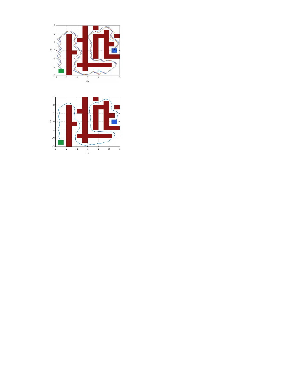
From Noisy Data to Hierarchical Control: A Model-Order -Reduction Frame work Behrad Samari, Henrik Sandberg, Karl H. Johansson, and Abolf azl Lav aei Abstract — This paper develops a direct data-driven frame- work for constructing reduced-order models (R OMs) of discrete-time linear dynamical systems with unknown dynamics and process disturbances. The proposed scheme enables con- troller synthesis on the ROM and its r efinement to the original system by an interface function designed using noisy data. T o achie ve this, the notion of simulation functions (SFs) is employed to establish a formal r elation between the original system and its R OM, yielding a quantitative bound on the mismatch between their output trajectories. T o construct such relations and interface functions, we rely on data collected from the unknown system. In particular , using noise-corrupted input–state data gathered along a single trajectory of the system, and without identifying the original dynamics, we propose data-dependent conditions, cast as a semidefinite pro- gram, for the simultaneous construction of ROMs, SFs, and interface functions. Through a case study , we demonstrate that data-driven controller synthesis on the ROM, combined with controller refinement via the interface function, enables the enfor cement of complex specifications beyond stability . I . I N T RO D U C T I O N Model order reduction (MOR) provides a systematic ap- proach for replacing a high-dimensional dynamical system with a lo wer-dimensional model that preserves the essential characteristics of the original system. Such simplified models are in v aluable, as they facilitate system analysis and con- troller synthesis while alleviating the computational burden associated with high dimensionality [ 1 ], which particularly arises in emerging applications dri ven by the increasing complexity of modern engineering systems. Despite these advantages, deriving reliable reduced-order models (R OMs) remains demanding, especially when the system is subject to process disturbances. The problem becomes e ven more challenging when an explicit model of the underlying system is unav ailable, a scenario that is often unav oidable in practice. In this conte xt, the literature adopts two main perspectives [ 2 ]: (i) combining system identifica- tion with model-based approaches to obtain R OMs, kno wn as indirect frameworks, or (ii) designing ROMs directly from data without an intermediate modeling step, kno wn as direct approaches. Bypassing the system identification stage can offer significant advantages, particularly when the system cannot be uniquely modeled [ 3 ], which is typically the case when the unknown system is subject to process disturbances. B. Samari and A. Lav aei are with the School of Computing, Newcastle Univ ersity , NE4 5TG Newcastle Upon T yne, United Kingdom (e-mails: { b.samari2,abolfazl.lavaei } @newcastle.ac.uk ). H. Sandberg and K. H. Johansson are with the Department of Decision and Control Systems, KTH Royal Institute of T echnology , SE-100 44 Stockholm, Sweden. They are also affiliated with Digital Futures (e-mails: { hsan,kallej } @kth.se ). Howe v er , establishing correctness guarantees becomes more challenging, since all conclusions must be drawn directly from data without relying on an explicit model. Related Literature and Core Contribution. MOR tech- niques, whether employed in model-based or data-dri ven settings, can be broadly categorized into three main groups, with our approach falling under the third cate gory: (i) energy- based approaches, such as balanced truncation [ 4 ]–[ 7 ] and Hankel-norm methods [ 8 ], [ 9 ]; (ii) Krylov-based methods, which rely on interpolation and/or moment matching [ 10 ]– [ 13 ]; and (iii) approaches grounded in the notion of simu- lation functions (SFs), where a similarity relation between the original high-dimensional system and its corresponding R OM is established [ 14 ]–[ 17 ]. Sev eral insightful data-driv en MOR results have been dev eloped within the first two categories. In the first cate- gory , [ 18 ] proposes a balanced truncation method based on persistently exciting data, [ 19 ] introduces a reformulation of balanced truncation via the estimation of Gramian-related quantities, and [ 20 ] presents a framework operating on noisy data under a known noise model. In the second category , [ 21 ] proposes a data-driv en MOR frame work based on time- domain measurements. Using swapped interconnection, [ 22 ] dev elops an algorithm that asymptotically estimates an arbi- trary number of moments from a single time-domain sample. More recently , [ 23 ] constructs ROMs from input–output data that achieve moment matching ev en when both the system and the signal generator are unknown, and [ 24 ] explores artificial neural networks for data-driven moment matching. While in valuable, the aforementioned studies are primarily suited for stability and input–output behavior analysis. In such framew orks, the same input is typically applied to both the original system and its R OM, which impedes their applicability to enforcing complex specifications, e.g . , safety , reachability , and reach-while-av oid. In contrast, approaches in the third category permit different inputs for the original system and its R OM while providing trajectory-wise bounds on their output mismatch. Specifically , a control input de- signed for the ROM is refined through an interface function into a control input for the original system, ensuring that the latter satisfies the specification fulfilled by the R OM, up to a guaranteed error bound [ 25 ]. W ithin the third category , to the best of our knowledge, this paper proposes the first direct data-driven method for constructing ROMs of discrete-time linear dynamical sys- tems with unknown models and process disturbances, while also establishing formal relations between the original system and its R OM using SFs and designing interface functions for control refinement. While the work in [ 26 ] also belongs to the third category , it focuses on continuous-time linear dynamical systems and does not account for process dis- turbances or noise in the collected data. In contrast, the present framew ork explicitly incorporates process distur- bances, which naturally giv e rise to noise-corrupted data. More importantly , while [ 26 ] combines direct and indirect data-driv en techniques (indirect for implicitly identifying the system matrices required for the interface function and certain equality conditions, and direct for the SF learning from data), the proposed approach is fully direct and does not inv olve any system identification. Finally , our framew ork requires only a single set of noise-corrupted input–state data, whereas [ 26 ] relies on two datasets, one of which must be collected under zero input, resulting in more demanding data requirements. W e also note that, while [ 27 ] falls within the third category by considering noise-corrupted data, it is tailored to continuous-time systems and does not account for process disturbances, in contrast to the current framework. Accordingly , the proof steps and the main constraint in ( 13f ) are substantially distinct from those in [ 27 ]. Moreov er , the closeness guarantee in ( 4 ) and the associated parameters in ( 15 ) are deri ved differently from those in [ 27 ]. Notation. The identity matrix of dimension n × n is denoted by I n , whereas 1 n represents the n -dimensional vector whose entries are all equal to one. Like wise, 𝟘 n × m denotes the zero matrix of dimension n × m , while 𝟘 n refers to the zero vector in R n . Given N vectors x i ∈ R n , the matrix X = [ x 1 . . . x N ] is formed by stacking these vectors as columns and therefore has dimension n × N . The Euclidean norm of a vector x ∈ R n is denoted by | x | , whereas ∥ P ∥ denotes the induced 2 -norm of a matrix P . For a symmetric matrix P , the notation P ≻ 0 ( P ⪰ 0 ) signifies that P is positiv e (semi)definite, whereas P ≺ 0 ( P ⪯ 0 ) denotes that P is negati ve (semi)definite. For a symmetric matrix P , the smallest and largest eigen v alues are denoted by λ min ( P ) and λ max ( P ) , respectiv ely . In a symmetric matrix, the symbol ⋆ denotes the transposed entry appearing in the corresponding symmetric position. The rank of a matrix A is denoted by rank( A ) . For a given matrix A , a ∈ col( A ) indicates that the vector a belongs to the column space of A . For a function f : N ≥ 0 → R n , we define | f | ∞ : = sup k ∈ N ≥ 0 | f ( k ) | . I I . P RO B L E M F O R M U L AT I O N A. System and R OM Descriptions W e consider a class of discrete-time linear control systems subject to process disturbances, formally defined as follo ws. Definition 2.1: A discrete-time linear control system (dt- LCS) is specified by the tuple Σ = ( X , U , Y , W , A, B , I n ) , where X ⊆ R n , U ⊆ R m , and Y , W ⊆ R n denote the sets of states, inputs, outputs, and disturbances of the system, respectively . The matrices A ∈ R n × n and B ∈ R n × m represent the system and input matrices that are both unknown . All state v ariables of Σ are directly measurable, which is reflected by the output matrix I n , i.e. , Y = X . For a giv en initial state x (0) = x ∈ X , input sequence ν : N ≥ 0 → U , and disturbance sequence ϖ : N ≥ 0 → W , the state and output of Σ ev olve for all k ∈ N ≥ 0 as Σ : ( x ( k + 1) = Ax ( k ) + B ν ( k ) + ϖ ( k ) , y ( k ) = x ( k ) . (1) For any initial state x ∈ X , input sequence ν : N ≥ 0 → U , and disturbance sequence ϖ : N ≥ 0 → W , the sequence x x ν ϖ : N ≥ 0 → X denotes the resulting state trajectory of Σ , while y x ν ϖ = x x ν ϖ denotes the associated output trajectory . The dt-LCS Σ in Definition 2.1 is construed as a system with an unknown model since the matrices A and B are not av ailable, a situation that commonly arises in many practical applications. The follo wing definition formally introduces the R OM associated with the dt-LCS Σ . Definition 2.2: A ROM of the dt-LCS Σ in Definition 2.1 is represented by the tuple ˆ Σ = ( ˆ X , ˆ U , ˆ Y , ˆ A, ˆ B , ˆ C ) , where ˆ X ⊂ R ˆ n , ˆ U ⊂ R ˆ m , and ˆ Y ⊂ R n denote the compact state, input, and output sets of the ROM, respecti vely . The matrices ˆ A ∈ R ˆ n × ˆ n , ˆ B ∈ R ˆ n × ˆ m , and ˆ C ∈ R n × ˆ n correspond to the system, input, and output matrices that are to be constructed, with potentially ˆ n ≪ n . Giv en an initial state ˆ x (0) = ˆ x ∈ ˆ X and an input sequence ˆ ν : N ≥ 0 → ˆ U , the state and output of ˆ Σ e volv e for all k ∈ N ≥ 0 according to ˆ Σ : ( ˆ x ( k + 1) = ˆ A ˆ x ( k ) + ˆ B ˆ ν ( k ) , ˆ y ( k ) = ˆ C ˆ x ( k ) . (2) For any initial condition ˆ x ∈ ˆ X and input sequence ˆ ν : N ≥ 0 → ˆ U , the sequences ˆ x ˆ x ˆ ν : N ≥ 0 → ˆ X and ˆ y ˆ x ˆ ν : N ≥ 0 → ˆ Y denote the state and output trajectories of ˆ Σ . Equipped with the definitions of the dt-LCS Σ and its R OM ˆ Σ , the following subsection establishes a relation between them using the notion of SFs, which is subsequently utilized to derive a quantitati ve bound on the closeness of their output trajectories. B. Simulation Functions SFs are defined on the Cartesian product of X and ˆ X to measure the proximity between the output trajectories of Σ and ˆ Σ . Specifically , SFs can be used to guarantee that the mismatch between the outputs of the two systems remains within a prescribed error bound. W e formally present this notion in the subsequent definition, adapted from the one in [ 28 ]. Definition 2.3: Giv en Σ = ( X , U , Y , W , A, B , I n ) and its R OM ˆ Σ = ( ˆ X , ˆ U , ˆ Y , ˆ A, ˆ B , ˆ C ) , a function S : X × ˆ X → R ≥ 0 is called an SF from ˆ Σ to Σ if there exist constants α, ρ, ψ ∈ R > 0 , and 0 < κ < 1 , such that • ∀ x ∈ X , ∀ ˆ x ∈ ˆ X , α | x − ˆ C ˆ x | 2 ≤ S ( x, ˆ x ) , (3a) • ∀ x ∈ X , ∀ ˆ x ∈ ˆ X , ∀ ˆ u ∈ ˆ U , ∃ u ∈ U such that, for all w ∈ W , one has S ( x + , ˆ x + ) ≤ κ S ( x, ˆ x ) + ρ | ˆ u | 2 + ψ , (3b) with x + : = Ax + B u + w and ˆ x + : = ˆ A ˆ x + ˆ B ˆ u . It is w orth noting that condition ( 3b ) suggests the e xistence of a function u = g k ( x, ˆ x, ˆ u ) that fulfills this condition. This function, referred to as the interface function, establishes a link between the input sequences ν and ˆ ν , thereby enabling the refinement of a control input designed for ˆ Σ into an input applicable to Σ . In Section III , we design such an interface function purely from data as one of the main contributions of the paper . W e also note that the notion of SFs introduced in Definition 2.3 essentially con ve ys that when the output trajectories of Σ and ˆ Σ originate from initial points that are adequately close (cf., condition ( 3a )), they retain closeness as time e volv es (cf., condition ( 3b )) [ 29 ]. The following theorem highlights the significance of the notion of SFs by formally quantifying the error between the output trajectories of Σ and ˆ Σ . Theor em 2.4: Giv en Σ = ( X , U , Y , W , A, B , I n ) and its R OM ˆ Σ = ( ˆ X , ˆ U , ˆ Y , ˆ A, ˆ B , ˆ C ) , let S be an SF from ˆ Σ to Σ . Then, for any initial states x ∈ X and ˆ x ∈ ˆ X , any disturbance sequence ϖ : N ≥ 0 → W , and any input sequence ˆ ν : N ≥ 0 → ˆ U , there exists an input sequence ν : N ≥ 0 → U such that, for all k ∈ N ≥ 0 : | y x ν ϖ ( k ) − ˆ y ˆ x ˆ ν ( k ) | ≤ s S (x , ˆ x) α + ρ | ˆ ν | 2 ∞ + ψ α (1 − κ ) . (4) Pr oof: W e first establish the existence of an input sequence ν : N ≥ 0 → U for the original system Σ corre- sponding to the given input sequence ˆ ν : N ≥ 0 → ˆ U of the R OM ˆ Σ . This follows from condition ( 3b ). In particular , at each time step k ∈ N ≥ 0 , given the current states x ( k ) and ˆ x ( k ) , as well as the input ˆ ν ( k ) , condition ( 3b ) ensures the existence of an input ν ( k ) satisfying the required inequality . By selecting ν ( k ) in this way at every time step, one obtains a well-defined input sequence ν : N ≥ 0 → U along the ev olution of the trajectories. This construction remains valid for the disturbance sequence ϖ , since condition ( 3b ) holds for all disturbances in W . T o proceed further with the proof, let V ( k ) : = S ( x ( k ) , ˆ x ( k )) for all k ∈ N ≥ 0 , for the sake of simpler notation. According to condition ( 3b ), one has V ( k + 1) = S ( x ( k + 1) , ˆ x ( k + 1)) ≤ κV ( k ) + ρ | ˆ ν ( k ) | 2 + ψ . Since for all k ∈ N ≥ 0 , one has | ˆ ν ( k ) | ≤ | ˆ ν | ∞ , we get V ( k + 1) ≤ κV ( k ) + ρ | ˆ ν | 2 ∞ + ψ , ∀ k ∈ N ≥ 0 . (5) By iterating ( 5 ), for e very k ≥ 1 , one gets V ( k ) ≤ κV ( k − 1) + ρ | ˆ ν | 2 ∞ + ψ ≤ κ  κV ( k − 2) + ρ | ˆ ν | 2 ∞ + ψ  + ρ | ˆ ν | 2 ∞ + ψ . . . ≤ κ k V (0) + k − 1 X j =0 κ k − 1 − j  ρ | ˆ ν | 2 ∞ + ψ  = κ k S (x , ˆ x) +  ρ | ˆ ν | 2 ∞ + ψ  k − 1 X j =0 κ j . Since 0 < κ < 1 , one has P k − 1 j =0 κ j = 1 − κ k 1 − κ ≤ 1 1 − κ , and κ k ≤ 1 . Therefore, we get V ( k ) ≤ S (x , ˆ x) + ρ | ˆ ν | 2 ∞ + ψ 1 − κ , ∀ k ∈ N ≥ 0 . (6) On the other hand, by ( 3a ), for all k ∈ N ≥ 0 , we ha ve α | x ( k ) − ˆ C ˆ x ( k ) | 2 ≤ S ( x ( k ) , ˆ x ( k )) = V ( k ) . (7) Using the output equations in ( 1 ) and ( 2 ), namely , y ( k ) = x ( k ) and ˆ y ( k ) = ˆ C ˆ x ( k ) , inequality ( 7 ) becomes α | y ( k ) − ˆ y ( k ) | 2 ≤ V ( k ) . Combining this with ( 6 ) yields α | y ( k ) − ˆ y ( k ) | 2 ≤ S (x , ˆ x) + ρ | ˆ ν | 2 ∞ + ψ 1 − κ , and therefore, one has | y ( k ) − ˆ y ( k ) | ≤ s S (x , ˆ x) α + ρ | ˆ ν | 2 ∞ + ψ α (1 − κ ) , ∀ k ∈ N ≥ 0 . Recall that y ( k ) = y x ν ϖ ( k ) and ˆ y ( k ) = ˆ y ˆ x ˆ ν ( k ) , thereby concluding the proof. Remark 2.5: The term ψ in ( 3b ) allows one to explicitly account for the effect of noise in the collected data caused by the process disturbances acting on the dt-LCS Σ . Howe v er , according to the bound in ( 4 ), large values of ψ directly increase the mismatch between the output trajectories of Σ and ˆ Σ . Hence, reducing ψ is an important design objectiv e, as it leads to a tighter closeness guarantee. Similarly , smaller values of ρ and lar ger v alues of α further tighten the bound in ( 4 ). These objectiv es are explicitly taken into account in Theorem 3.3 . In addition, enforcing S (x , ˆ x) = 0 remov es the first term in ( 4 ), thereby yielding a tighter closeness guarantee. Since Theorem 2.4 provides a quantitati ve bound on the mismatch between the output trajectories of Σ and ˆ Σ , the proposed framework can be employed to enforce a broad class of specifications beyond stability , including safety , reachability , and reach-while-av oid. In particular , a formal controller can first be synthesized for the lower -dimensional R OM ˆ Σ so that the desired specification is satisfied. Then, by means of a suitably designed interface function, the R OM controller can be refined for the original higher-dimensional system Σ , while ensuring that the mismatch between the output trajectories of the two systems remains bounded as in ( 4 ). This, in turn, enables Σ to satisfy the specification of interest up to the guaranteed closeness error . Despite the advantages of SFs, constructing them requires exact kno wledge of system matrices, as A and B explicitly appear in ( 3b ). In this paper , howe v er , these matrices are unknown, which constitutes the main challenge. The next section proposes a direct data-dri ven framew ork to address this problem. I I I . D A T A - D R I V E N M E T H O D O L O G Y A. Data Collection W e first perform a finite-horizon experiment on the dt- LCS Σ ov er the interval [0 , T ] , where T ∈ N ≥ 1 denotes the experiment horizon, and collect the input–state data X =  x (0) x (1) . . . x ( T − 1)  ∈ R n × T , (8a) U =  ν (0) ν (1) . . . ν ( T − 1)  ∈ R m × T , (8b) X + =  x (1) x (2) . . . x ( T )  ∈ R n × T , (8c) W =  ϖ (0) ϖ (1) . . . ϖ ( T − 1)  ∈ R n × T , (8d) where W is unknown and cannot be measured directly . Since W af fects both X and X + through the system dynamics, the collected data are noise-corrupted. While W is unknown, we impose the following assumption [ 30 ], which indicates that the disturbance is bounded. Assumption 1: There exists a known constant ε ∈ R > 0 such that, for all w ∈ W , | w | ≤ ε. Notice that, under Assumption 1 , one has W W ⊤ = T − 1 X k =0 ϖ ( k ) ϖ ⊤ ( k ) ⪯ T − 1 X k =0 | ϖ ( k ) | 2 I n ⪯ ∆ , (9) where ∆ : = ε 2 T I n . The first inequality follo ws from ϖ ( k ) ϖ ⊤ ( k ) ⪯ | ϖ ( k ) | 2 I n , ∀ k ∈ { 0 , . . . , T − 1 } , whereas the second one follows from Assumption 1 and the fact that ϖ ( k ) ∈ W for all k ∈ { 0 , . . . , T − 1 } . W e note that the bound in ( 9 ) plays a key role in the subsequent analysis, as it allows us to provide correctness guarantees for all system matrices consistent with the measured data and the assumed bound in Assumption 1 . W e also impose the following assumption on the collected data in ( 8 ), which facilitates the feasibility analysis of the proposed frame work (cf., Section IV -A ). Assumption 2: The collected data satisfy the rank condi- tion rank( H ) = m + n, (10) where H =  U ⊤ X ⊤  ⊤ . Remark 3.1: Assumption 2 , which is closely related to the notion of persistency of excitation [ 31 ], essentially serves as a data richness condition, ensuring that the collected data are sufficiently informativ e for the subsequent analysis. When the noise is suf ficiently small, a suf ficient condition for Assumption 2 to hold is that the input sequence is persistently exciting of order n + 1 and that the pair ( A, B ) is controllable [ 31 ]. Moreover , the rank condition ( 10 ) implies that the experiment horizon must at least satisfy T ≥ m + n . B. Data-Driven R OM and SF Construction W ith the data collection procedure specified, we now turn to the dev elopment of our direct data-driv en framew ork. T o construct an SF satisfying the conditions in Definition 2.3 , we restrict attention to quadratic functions of the form S ( x, ˆ x ) = ( x − R ˆ x ) ⊤ P ( x − R ˆ x ) , where P ≻ 0 , and R ∈ R n × ˆ n denotes the r econstruction matrix . Giv en the adopted quadratic structure of the SF , the term x + − R ˆ x + naturally arises in condition ( 3b ). Motiv ated by this observ ation, the following lemma deriv es a suitable pa- rameterization of this term while simultaneously presenting the proposed structure of the interface function. Lemma 3.2: Giv en Σ = ( X , U , Y , W , A, B , I n ) and its R OM ˆ Σ = ( ˆ X , ˆ U , ˆ Y , ˆ A, ˆ B , ˆ C ) , let S : =  B A  , and the interface function be structured as u = GP ( x − R ˆ x ) + E ˆ x + D ˆ u, (11) where G ∈ R m × n , P ∈ R n × n , R ∈ R n × ˆ n , E ∈ R m × ˆ n , and D ∈ R m × ˆ m . Accordingly , one obtains the follo wing parameterization: x + − R ˆ x + = S  GP I n  ( x − R ˆ x ) +  S  E R  − R ˆ A  ˆ x +  S  D 𝟘 n × ˆ m  − R ˆ B  ˆ u + w. (12) Pr oof: Giv en that x + : = Ax + B u + w , ˆ x + : = ˆ A ˆ x + ˆ B ˆ u , and S : =  B A  , and considering the interface function in ( 11 ), one has x + − R ˆ x + = Ax + B u + w − R ( ˆ A ˆ x + ˆ B ˆ u ) ( 11 ) = Ax + B GP ( x − R ˆ x ) + B E ˆ x + B D ˆ u + w − R ( ˆ A ˆ x + ˆ B ˆ u ) = A ( x − R ˆ x ) + B GP ( x − R ˆ x ) + AR ˆ x + B E ˆ x + B D ˆ u + w − R ˆ A ˆ x − R ˆ B ˆ u = ( A + B GP )( x − R ˆ x ) + ( AR + B E − R ˆ A ) ˆ x + ( B D − R ˆ B ) ˆ u + w =  B A   GP I n  ( x − R ˆ x ) +   B A   E R  − R ˆ A  ˆ x +   B A   D 𝟘 n × ˆ m  − R ˆ B  ˆ u + w, where the third equality is obtained by addition and subtrac- tion of the term AR ˆ x , leading to ( 12 ) with S : =  B A  , thereby concluding the proof. W ith the interface function in ( 11 ) and the parameteriza- tion in ( 12 ) at hand, we no w propose the following theorem as the main result of the paper, which allows the interface function ( 11 ) and the SF S ( x, ˆ x ) to be constructed simul- taneously from noise-corrupted data, without identifying the system matrices. Theor em 3.3: Giv en Σ = ( X , U , Y , W , A, B , I n ) and its R OM ˆ Σ = ( ˆ X , ˆ U , ˆ Y , ˆ A, ˆ B , ˆ C ) with ˆ C = R , let Assump- tions 1 and 2 hold. If there exist decision variables β ∈ R > 0 , K 1 ∈ R T × ˆ n , K 2 ∈ R T × ˆ m , ¯ P ∈ R n × n , with ¯ P ≻ 0 , G ∈ R m × n , and ¯ µ ∈ R ≥ 0 such that, for gi ven η , µ i ∈ R > 0 for all i ∈ { 1 , . . . , 6 } , 0 < κ < 1 , ˆ A , and ˆ B , the semidefinite program (SDP) min ¯ µ,K 1 ,K 2 , G, ¯ P ,β ∥ K 1 ∥ + ∥ K 2 ∥ + ∥ X + K 2 − X K 1 ˆ B ∥ + β (13a) s . t . 1 ⊤ T K 1 1 ˆ n ≥ η , (13b) ¯ P ⪯ β I n , (13c) X + K 1 = X K 1 ˆ A, (13d) X K 2 = 𝟘 n × ˆ m , (13e) Q 1 − ¯ µ Q 2 ⪰ 0 (13f) has a solution, where Q 1 : =     κ ¯ P 𝟘 n × ( n + m ) 𝟘 n × n ⋆ 𝟘 ( n + m ) × ( n + m )  G ¯ P  ⋆ ⋆ 1 1+ P 3 i =1 µ i ¯ P     , (14a) Q 2 : =   ∆ − X + X ⊤ + X + H ⊤ 𝟘 n × n ⋆ − H H ⊤ 𝟘 ( n + m ) × n ⋆ ⋆ 𝟘 n × n   , (14b) with H =  U ⊤ X ⊤  ⊤ , then S ( x, ˆ x ) = ( x − R ˆ x ) ⊤ P ( x − R ˆ x ) is an SF from ˆ Σ to Σ , with R : = X K 1 , P : = ¯ P − 1 , α : = λ min ( P ) , and ρ : =  1 + 1 µ 2 + 1 µ 4 + µ 6  λ max ( P ) Z , (15a) ψ : =  1 + 1 µ 1 + µ 4 + µ 5  λ max ( P ) λ max (∆) ∥ K 1 ∥ 2 max ˆ x ∈ ˆ X | ˆ x | 2 +  1 + 1 µ 3 + 1 µ 5 + 1 µ 6  λ max ( P ) ε 2 , (15b) where Z : = ( ∥ X + K 2 − X K 1 ˆ B ∥ + p λ max (∆) ∥ K 2 ∥ ) 2 . Moreov er , the corresponding interf ace function is given by ( 11 ), with E : = U K 1 and D : = U K 2 . Pr oof: The proof is carried out in two steps. Under the SDP ( 13 ), the first step illustrates that constraint ( 3a ) is satisfied, whereas the second, and technically more inv olved, step establishes constraint ( 3b ). T o continue with the first step, recall that ˆ C = R , which yields | x − ˆ C ˆ x | 2 = | x − R ˆ x | 2 . Moreov er , since λ min ( P ) | x − R ˆ x | 2 ≤ ( x − R ˆ x ) ⊤ P ( x − R ˆ x ) = S ( x, ˆ x ) , it follows that ( 3a ) holds with α : = λ min ( P ) . This completes the first stage of the proof. T o continue with the second step, considering S ( x, ˆ x ) = ( x − R ˆ x ) ⊤ P ( x − R ˆ x ) , one has S ( x + , ˆ x + ) = ( x + − R ˆ x + ) ⊤ P ( x + − R ˆ x + ) ( 12 ) =  S  G P − 1  P ( x − R ˆ x ) + ♣ z }| {  S  E R  − R ˆ A  ˆ x + ♠ z }| {  S  D 𝟘 n × ˆ m  − R ˆ B  ˆ u + w  ⊤ P ( ∗ ) , (16) where ( ∗ ) represents the expression appearing in the first parenthesis in ( 16 ). Observe that, according to the dt-LCS Σ in ( 1 ), the data collected in ( 8 ) satisfy X + = AX + B U + W = S H + W, (17) where S : =  B A  and H : =  U ⊤ X ⊤  ⊤ . W e first restrict our attention to the term “ ♣ ” in ( 16 ). Inspired by the insightful work [ 32 ], and recalling that R : = X K 1 and E : = U K 1 , under constraint ( 13d ), one has X + K 1 = X K 1 ˆ A ( 17 ) ⇐ ⇒ S H K 1 + W K 1 = X K 1 ˆ A ⇐ ⇒ S  U K 1 X K 1  + W K 1 = X K 1 ˆ A ⇐ ⇒ S  E R  + W K 1 = R ˆ A. Hence, the term “ ♣ ” in ( 16 ) can be substituted by − W K 1 . Focusing on the term “ ♠ ” in ( 16 ), and recalling that D : = U K 2 and R : = X K 1 , under constraint ( 13e ), it follows that S  D 𝟘 n × ˆ m  − R ˆ B ( 13e ) = S H z }| {  U X  K 2 − R ˆ B ( 17 ) = ( X + − W ) K 2 − X K 1 ˆ B = N 1 z }| { ( X + K 2 − X K 1 ˆ B ) N 2 z }| { − W K 2 . (18) Therefore, the term “ ♠ ” in ( 16 ) can be replaced by ( 18 ). Incorporating these substitutions, one can rewrite ( 16 ) as S ( x + , ˆ x + ) =  T 1 z }| { S  G P − 1  P ( x − R ˆ x ) T 2 z }| { − W K 1 ˆ x + T 3 z }| { ( N 1 + N 2 ) ˆ u + T 4 z}|{ w  ⊤ P ( ∗ ) = 4 X i =1 T ⊤ i P T i + 4 X j =2 2 T ⊤ 1 P T j + 4 X z =3 2 T ⊤ 2 P T z + 2 T ⊤ 3 P T 4 . Notice that for all i, j ∈ { 1 , . . . , 4 } , one can re write 2 T ⊤ i P T j as 2( √ P T i ) ⊤ ( √ P T j ) . Considering this, we next employ the Cauchy–Schwarz inequality , i.e. , a ⊤ b ≤ | a || b | for any a, b ∈ R n , and subsequently apply Y oung’ s inequality , i.e. , | a || b | ≤ µ i 2 | a | 2 + 1 2 µ i | b | 2 for any µ i ∈ R > 0 for all i ∈ { 1 , . . . , 6 } , which yields 4 X j =2 2 T ⊤ 1 P T j ≤ 3 X i =1 µ i T ⊤ 1 P T 1 + 1 µ 1 T ⊤ 2 P T 2 + 1 µ 2 T ⊤ 3 P T 3 + 1 µ 3 T ⊤ 4 P T 4 , 4 X z =3 2 T ⊤ 2 P T z ≤ 5 X i =4 µ i T ⊤ 2 P T 2 + 1 µ 4 T ⊤ 3 P T 3 + 1 µ 5 T ⊤ 4 P T 4 , and 2 T ⊤ 3 P T 4 ≤ µ 6 T ⊤ 3 P T 3 + 1 µ 6 T ⊤ 4 P T 4 . Consequently , we have S ( x + , ˆ x + ) ≤  1 + 3 X i =1 µ i  T ⊤ 1 P T 1 +  1 + 1 µ 1 + µ 4 + µ 5  T ⊤ 2 P T 2 +  1 + 1 µ 2 + 1 µ 4 + µ 6  T ⊤ 3 P T 3 +  1 + 1 µ 3 + 1 µ 5 + 1 µ 6  T ⊤ 4 P T 4 . W e no w proceed to deri ve upper bounds for T ⊤ 2 P T 2 , T ⊤ 3 P T 3 , and T ⊤ 4 P T 4 , which eventually lead to ρ and ψ as specified in ( 15 ). T o this end, we hav e T ⊤ 2 P T 2 = ˆ x ⊤ K ⊤ 1 W ⊤ P W K 1 ˆ x ≤ λ max ( P ) ˆ x ⊤ K ⊤ 1 W ⊤ W K 1 ˆ x ≤ λ max ( P ) λ max ( W ⊤ W ) ˆ x ⊤ K ⊤ 1 K 1 ˆ x = λ max ( P ) λ max ( W W ⊤ ) ˆ x ⊤ K ⊤ 1 K 1 ˆ x ( 9 ) ≤ λ max ( P ) λ max (∆) ∥ K 1 ∥ 2 | ˆ x | 2 ≤ λ max ( P ) λ max (∆) ∥ K 1 ∥ 2 max ˆ x ∈ ˆ X | ˆ x | 2 . Follo wing the same rationale and recalling Assumption 1 , one has T ⊤ 4 P T 4 ≤ λ max ( P ) ε 2 . As for T ⊤ 3 P T 3 , we ha ve T ⊤ 3 P T 3 = ˆ u ⊤ ( N 1 + N 2 ) ⊤ P ( N 1 + N 2 ) ˆ u ≤ λ max ( P ) ∥N 1 + N 2 ∥ 2 | ˆ u | 2 ≤ λ max ( P )( ∥N 1 ∥ + ∥N 2 ∥ ) 2 | ˆ u | 2 ( 18 ) ≤ λ max ( P )( ∥N 1 ∥ + ∥ W ∥∥ K 2 ∥ ) 2 | ˆ u | 2 ( 9 ) ≤ λ max ( P ) Z z }| { ( ∥N 1 ∥ + p λ max (∆) ∥ K 2 ∥ ) 2 | ˆ u | 2 , where, for the last inequality , we use ∥ W ∥ 2 = λ max ( W W ⊤ ) ( 9 ) ≤ λ max (∆) ⇒ ∥ W ∥ ≤ p λ max (∆) . Accordingly , one obtains S ( x + , ˆ x + ) ≤  1 + 3 X i =1 µ i  T ⊤ 1 P T 1 +  1 + 1 µ 1 + µ 4 + µ 5  λ max ( P ) λ max (∆) ∥ K 1 ∥ 2 max ˆ x ∈ ˆ X | ˆ x | 2 +  1 + 1 µ 2 + 1 µ 4 + µ 6  λ max ( P ) Z | ˆ u | 2 +  1 + 1 µ 3 + 1 µ 5 + 1 µ 6  λ max ( P ) ε 2 , establishing ρ and ψ as in ( 15 ) (cf., condition ( 3b )). T o proceed with the proof, it remains to show that under constraint ( 13f ), the inequality  1 + 3 X i =1 µ i  T ⊤ 1 P T 1 ≤ κ ( x − R ˆ x ) ⊤ P ( x − R ˆ x ) (19) holds. T o sho w this, recalling P = P ⊤ ≻ 0 , it is sufficient to illustrate that κP −  1 + 3 X i =1 µ i  P  G P − 1  ⊤ S ⊤ P S  G P − 1  P ⪰ 0 . Pre-multiplying and post-multiplying this by P − 1 , one gets κP − 1 −  1 + 3 X i =1 µ i   G P − 1  ⊤ S ⊤ P S  G P − 1  ⪰ 0 . Utilizing the Schur complement, this expression can be equiv alently rewritten as   1 1+ P 3 i =1 µ i P − 1 S  G P − 1  ⋆ κP − 1   ⪰ 0 ⇐ ⇒    κP − 1  G P − 1  ⊤ S ⊤ ⋆ 1 1+ P 3 i =1 µ i P − 1    ⪰ 0 ⇐ ⇒ κP − 1 −  1 + 3 X i =1 µ i  S  G P − 1  P  G P − 1  ⊤ S ⊤ ⪰ 0 , and, subsequently , as  I n S ⊤  ⊤ M 1 z }| {   κP − 1 𝟘 n × ( n + m ) ⋆ −  1 + P 3 i =1 µ i   G P − 1  P  G P − 1  ⊤    I n S ⊤  ⪰ 0 . (20) Satisfying ( 20 ) presents two challenges: (i) it depends on the unknown system matrices S , and (ii) its second diagonal block is nonlinear , which obstructs solving it. T o overcome the first difficulty , we return to Assumption 1 together with the linear matrix inequality (LMI) ( 9 ). Specifically , the LMI ( 9 ) can be re written as ∆ ⪰ W W ⊤ ( 17 ) ⇐ ⇒ ∆ ⪰ ( X + − S H )( X + − S H ) ⊤ , which yields  I n S ⊤  ⊤ M 2 z }| {  ∆ − X + X ⊤ + X + H ⊤ ⋆ − H H ⊤   I n S ⊤  ⪰ 0 . (21) Since both LMIs ( 20 ) and ( 21 ) are quadratic in  I n S  ⊤ , the classical S-procedure [ 30 , Theorem 9] can be employed to enforce ( 20 ) while accounting for ( 21 ). In particular, this remov es the need for explicit knowledge of S , and ( 20 ) can be guaranteed pro vided that there e xists a multiplier ¯ µ ∈ R ≥ 0 such that M 1 − ¯ µ M 2 ⪰ 0 . (22) W ith the first challenge resolv ed, it remains to address the second one. For this purpose, the Schur complement can again be applied, which, recalling ¯ P = P − 1 , sho ws that ( 13f ) ⇐ ⇒ ( 22 ) . Therefore, under constraint ( 13f ), condition ( 19 ) is ensured, which completes the proof. Remark 3.4: Smaller values of ˆ n typically facilitate con- troller synthesis for ˆ Σ . The choice of ˆ n mainly depends on two aspects: (i) the specification imposed on Σ and (ii) the feasibility of achieving a meaningful closeness guarantee. For instance, if the objective concerns only the first two state variables of the original system ( e.g . , positions along the x - and y -axes), selecting ˆ n = 2 is desirable, since it enables direct control. If such a reduction does not yield a valid closeness guarantee, larger values of ˆ n should be considered progressiv ely until a suitable ˆ Σ is obtained. Remark 3.5: If R and ˆ A were to be designed simultane- ously , constraint ( 13d ) would become bilinear due to their product. Such an issue is inherent to SF-based methods and also appears in model-based settings (cf., condition (20a) in [ 15 ]). T o circumvent this issue, for a chosen ˆ n (cf., Remark 3.4 ), one can fix ˆ A and then solve the SDP ( 13 ). In practice, selecting ˆ A is straightforward; choosing it as a Schur matrix simplifies the control design for ˆ Σ . Moreov er, since Theorem 3.3 imposes no restriction on the structure of ˆ B , a natural choice is ˆ B = γ I ˆ n with γ ∈ R \{ 0 } (hence ˆ m = ˆ n ). This renders ˆ Σ fully actuated, which facilitates controller synthesis. Additionally , through its effect on the term ∥ X + K 2 − X K 1 ˆ B ∥ in ( 15a ), the parameter γ can be used to regulate ρ , and thus the closeness guarantee in ( 4 ). I V . D I S C U S S I O N A. F easibility Analysis of SDP ( 13 ) W e first note that constraints ( 13b ) and ( 13c ) are not intrinsic to the proposed framework. In particular , since K 1 = 𝟘 T × ˆ n is a tri vial yet undesirable solution of ( 13d ), constraint ( 13b ) is introduced solely to exclude this case. Like wise, constraint ( 13c ) is introduced, and β ∈ R > 0 is included in the cost function ( 13a ), to promote a potentially large v alue of α : = λ min ( P ) , thereby tightening the close- ness guarantee ( 4 ). Similarly , the inclusion of ∥ K 1 ∥ , ∥ K 2 ∥ , and ∥ X + K 2 − X K 1 ˆ B ∥ in the cost function ( 13a ) promotes solutions with smaller v alues of these norms, which can potentially reduce the v alues of ψ and ρ in ( 15 ), thereby further tightening the closeness guarantee ( 4 ). W e further note that constraint ( 13d ) alone is a homo- geneous system of linear equations and is therefore always feasible, since it admits the trivial solution K 1 = 𝟘 T × ˆ n . Moreov er , if T > n , which follows from Assumption 2 and Remark 3.1 when m ≥ 1 , then ( 13d ) has more unkno wns than scalar equalities, namely , T ˆ n unknowns and n ˆ n scalar equalities; hence, it admits a nontrivial solution. Under the same condition T > n , constraint ( 13e ) is also a homo- geneous system of linear equations and therefore is always feasible, while also admitting a nontrivial solution. W e also remark that Assumption 2 f acilitates the feasibility of condition ( 13f ). In fact, Assumption 2 implies that H has full ro w rank, and hence H H ⊤ ≻ 0 . Consequently , whenev er ¯ µ ∈ R > 0 , ¯ µH H ⊤ ≻ 0 . If Assumption 2 fails, then H H ⊤ becomes singular, and feasibility of ( 13f ), although still possible, requires the off-diagonal blocks coupled with ¯ µH H ⊤ to satisfy additional compatibility conditions; in par- ticular , their columns must belong to col( H H ⊤ ) . Therefore, Assumption 2 removes this structural difficulty whenev er ¯ µ ∈ R > 0 , thereby facilitating the satisfaction of ( 13f ). B. Scalability Analysis W e focus here on constraint ( 13f ), as it constitutes the main computationally demanding constraint. In particular , constraint ( 13f ) is an LMI of dimension (3 n + m ) × (3 n + m ) . While this size gro ws linearly with both n and m , it is typically dominated by the state dimension n . According to [ 33 ], such LMIs hav e approximate time and memory complexities of O ( n 6 . 5 ) and O ( n 4 ) , respectiv ely , which can be computationally demanding. W e note that, while energy- based and Krylov-based methods generally offer better scal- ability , the current setting can accommodate complex spec- ifications for which the aforementioned approaches are not typically applicable (cf., the case study), thereby offsetting this potential limitation. C. Limitations Similar to any methodology , the proposed framew ork has certain limitations, which can also be viewed as directions for future research. First, the current setting is specifically tailored to linear dynamical systems. W e note that, for a par- ticular class of nonlinear dynamical systems, [ 27 ] proposes a data-dri ven approach for constructing SFs and interface functions. Howe ver , the approach in [ 27 ] is developed for the continuous-time setting and, more importantly , does not account for process disturbances. This suggests that extending the present frame work to handle certain classes of nonlinear systems subject to process disturbances within the discrete-time setting would require further theoretical dev elopment. Second, the proposed data-driv en frame work requires input–state data and assumes that all state variables are directly measurable. Inspired by the recent work in [ 34 ], one potential direction is to extend the current framework to settings in which the state vector is partially measurable. V . S I M U L A T I O N R E S U LT S This section demonstrates the effecti veness of the pro- posed data-dri ven frame work. In particular, for a six- dimensional dt-LCS subject to process disturbances, we aim to construct a ROM of dimension two, design a controller for the R OM that satisfies a challenging reach-while-a void specification, and subsequently refine the synthesized con- troller back to the original system, thereby enabling the dt- LCS to satisfy the desired specification. It is worth noting that for the original dt-LCS, the direct design of such a controller using tools commonly employed in the formal methods community , such as SCOTS [ 35 ], is remarkably challenging, if not infeasible. In contrast, employing the proposed MOR frame work significantly facilitates this design task. W e performed all simulations using M A T L A B R2023b on a MacBook Pro (Apple M2 Max, 32 GB memory). W e consider a dt-LCS as in ( 1 ), where A =        0 . 82 0 . 10 0 0 0 0 0 0 . 78 0 . 12 0 0 0 0 0 0 . 75 0 . 10 0 0 0 0 0 0 . 72 0 . 08 0 0 0 0 0 0 . 70 0 . 10 0 . 05 0 0 0 0 0 . 68        , and B =  0 . 68 0 . 34 0 . 17 0 0 0 0 0 0 0 . 34 0 . 68 0 . 34  ⊤ , with both matrices being unknown. Moreover , as enabled by Assumption 1 , we assume that ε = 0 . 0014 is known. Accordingly , we conduct an experiment on the dt-LCS for data collection with a horizon of T = 300 . Consequently , one can compute ∆ = 5 . 88 × 10 − 4 I 6 according to ( 9 ). Follo wing Remark 3.5 , we choose ˆ A = 0 . 99 I 2 , ˆ B = 0 . 0001 I 2 . Moreov er , we set κ = 0 . 7 , µ 1 = 0 . 5 , µ 2 = 0 . 25 , µ 3 = 0 . 25 , µ 4 = 0 . 1 , µ 5 = 1 , and µ 6 = 1 . W e now proceed with solving the SDP ( 13 ), which yields ∥ K 1 ∥ = 0 . 0099 , ∥ K 2 ∥ = 1 . 2795 × 10 − 6 , ∥ X + K 2 − X K 1 ˆ B ∥ = 1 . 6699 × 10 − 4 , β = 30 . 5533 , ¯ µ = 9 . 9428 × 10 − 6 , and GP =  − 3 . 6392 4 . 6172 1 . 4406 0 . 40121 − 0 . 67234 2 . 1956 − 2 . 4812 − 2 . 1611 0 . 3313 − 0 . 86503 0 . 54923 − 0 . 78516  . Furthermore, we subsequently compute R =  0 . 5 0 − 0 . 375 − 1 . 1625 − 1 . 5359 − 0 . 5551 0 0 . 5 1 . 125 2 . 9374 3 . 9216 1 . 5898  ⊤ E =  0 . 1324 − 0 . 0735 − 0 . 5960 1 . 4963  , D = 10 − 3 ×  0 . 0404 0 . 0573 − 0 . 2619 0 . 5939  , forming the interface function as in ( 11 ). W e also obtain α = 2 . 2273 × 10 3 and λ max ( P ) = 6 . 8817 × 10 7 . Accordingly , one can compute ρ = 30 . 7155 . No w , considering ˆ X = [ − 6 , 6] 2 and ˆ U = [ − 6 , 6] 2 , we compute max ˆ x ∈ ˆ X | ˆ x | 2 = 72 and | ˆ ν | 2 ∞ ≤ 72 , yielding ψ = 2 . 1149 × 10 3 , and the value 2 . 545 for the bound in ( 4 ), noting that S (x , ˆ x) = 0 . The corresponding simulation results are depicted in Fig. 1 . As illustrated, the complex r each-while-avoid specification, which requires the system trajectories to start from the initial set , reach the target set , while av oiding collisions with the obstacles , is satisfied across all 5 simulation runs. V I . C O N C L U S I O N W e proposed a direct data-driven frame work for construct- ing R OMs of discrete-time linear dynamical systems with unknown dynamics and process disturbances. W e deriv ed data-dependent conditions for the simultaneous construction of R OMs, SFs, interface functions, and quantitativ e closeness guarantees directly from noise-corrupted input–state data collected along a single trajectory of the system. Future research will focus on extending the proposed framework to nonlinear systems and expanding it to incorporate input– output data. R E F E R E N C E S [1] A. C. Antoulas, Approximation of Lar ge-scale Dynamical Systems . SIAM, 2005. [2] F . D ¨ orfler , J. Coulson, and I. Marko vsky , “Bridging direct and indirect data-driv en control formulations via regularizations and relaxations, ” IEEE T ransactions on Automatic Control , vol. 68, no. 2, pp. 883–897, 2022. (a) Five original-system trajectories with different initial conditions (b) Original-system trajectory after applying a smoothing filter Fig. 1: (a) T rajectories of the dt-LCS for 5 simulation runs with different initial conditions, all satisfying the complex specification. (b) A representativ e trajectory after applying a smoothing filter to mitigate the zigzag behavior observed in (a), which arises from the SCOTS synthesis tool due to the chosen discretization parameter . A video of this simulation is av ailable at https://youtu.be/_cp93M1UmTc . [3] H. J. V an W aarde, J. Eising, H. L. Trentelman, and M. K. Camlibel, “Data informativity: A new perspecti ve on data-driv en analysis and control, ” IEEE T ransactions on Automatic Contr ol , vol. 65, no. 11, pp. 4753–4768, 2020. [4] B. Moore, “Principal component analysis in linear systems: Control- lability , observability , and model reduction, ” IEEE T ransactions on Automatic Contr ol , vol. 26, no. 1, pp. 17–32, 1981. [5] S. Prajna and H. Sandberg, “On model reduction of polynomial dynamical systems, ” in Pr oceedings of the 44th IEEE Conference on Decision and Control (CDC) , pp. 1666–1671, 2005. [6] H. Sandberg, “ An extension to balanced truncation with application to structured model reduction, ” IEEE Tr ansactions on Automatic Contr ol , vol. 55, no. 4, pp. 1038–1043, 2010. [7] B. Besselink, N. van de W ouw , J. M. Scherpen, and H. Nijmeijer, “Model reduction for nonlinear systems by incremental balanced truncation, ” IEEE T ransactions on Automatic Contr ol , vol. 59, no. 10, pp. 2739–2753, 2014. [8] K. Glover , “ All optimal Hankel-norm approximations of linear mul- tiv ariable systems and their L ∞ -error bounds, ” International Journal of Control , vol. 39, no. 6, pp. 1115–1193, 1984. [9] Y . Kaw ano and J. M. Scherpen, “Model reduction by differential balancing based on nonlinear Hankel operators, ” IEEE T ransactions on Automatic Contr ol , vol. 62, no. 7, pp. 3293–3308, 2016. [10] A. Astolfi, “Model reduction by moment matching for linear and nonlinear systems, ” IEEE T ransactions on Automatic Control , vol. 55, no. 10, pp. 2321–2336, 2010. [11] M. F . Shakib, G. Scarciotti, A. Y . Pogromsky , A. Pavlov , and N. van de W ouw , “Time-domain moment matching for multiple-input multiple- output linear time-inv ariant models, ” Automatica , vol. 152, 2023. [12] A. Moreschini and A. Astolfi, “Closed-loop interpolation by moment matching for linear and nonlinear systems, ” IEEE T ransactions on Automatic Contr ol , 2024. [13] M. F . Shakib, A. Moreschini, and G. Scarciotti, “Dissipati vity- preserving model reduction for linear systems using moment match- ing, ” European Journal of Contr ol , 2025. [14] A. Girard and G. J. Pappas, “Hierarchical control system design using approximate simulation, ” A utomatica , vol. 45, no. 2, pp. 566–571, 2009. [15] M. Zamani and M. Arcak, “Compositional abstraction for networks of control systems: A dissipativity approach, ” IEEE T ransactions on Contr ol of Network Systems , vol. 5, no. 3, pp. 1003–1015, 2017. [16] A. Lav aei, S. Soudjani, and M. Zamani, “Compositional construction of infinite abstractions for networks of stochastic control systems, ” Automatica , vol. 107, pp. 125–137, 2019. [17] A. Lav aei, S. Soudjani, and M. Zamani, “Compositional (in) finite abstractions for large-scale interconnected stochastic systems, ” IEEE T ransactions on Automatic Contr ol , vol. 65, no. 12, pp. 5280–5295, 2020. [18] P . Rapisarda and H. L. T rentelman, “Identification and data-driven model reduction of state-space representations of lossless and dis- sipativ e systems from noise-free data, ” Automatica , vol. 47, no. 8, pp. 1721–1728, 2011. [19] I. V . Gosea, S. Gugercin, and C. Beattie, “Data-dri ven balancing of linear dynamical systems, ” SIAM Journal on Scientific Computing , vol. 44, no. 1, pp. A554–A582, 2022. [20] A. M. Burohman, B. Besselink, J. M. A. Scherpen, and M. K. Cam- libel, “From data to reduced-order models via generalized balanced truncation, ” IEEE T ransactions on Automatic Contr ol , vol. 68, no. 10, pp. 6160–6175, 2023. [21] G. Scarciotti and A. Astolfi, “Data-driven model reduction by moment matching for linear and nonlinear systems, ” Automatica , vol. 79, pp. 340–351, 2017. [22] J. Mao and G. Scarciotti, “Data-driven model reduction by moment matching for linear systems through a swapped interconnection, ” in Pr oceedings of Eur opean Contr ol Conference (ECC) , pp. 1690–1695, 2022. [23] D. Bhattacharjee, A. Moreschini, and A. Astolfi, “Signal generator agnostic moment matching, ” IEEE Tr ansactions on Automatic Contr ol , 2025. [24] M. Scandella, D. Previtali, and A. Moreschini, “ Are artificial neural networks suitable for data-driven moment matching?, ” European J our- nal of Control , 2025. [25] A. Lavaei, S. Soudjani, A. Abate, and M. Zamani, “ Automated verification and synthesis of stochastic hybrid systems: A survey , ” Automatica , vol. 146, 2022. [26] B. Samari, A. Nejati, and A. Lav aei, “Model order reduction from data with certification, ” in Pr oceedings of the 64th IEEE Conference on Decision and Control (CDC) , pp. 5800–5805, 2025. [27] B. Samari, H. Sandberg, K. H. Johansson, and A. Lav aei, “Data- driv en model order reduction of nonlinear systems with noisy data, ” arXiv:2507.18131v2 , 2026. [28] A. J. van der Schaft, “Equiv alence of dynamical systems by bisim- ulation, ” IEEE T ransactions on Automatic Control , vol. 49, no. 12, pp. 2160–2172, 2004. [29] P . T abuada, V erification and Control of Hybrid Systems: A Symbolic Appr oach . Springer Science & Business Media, 2009. [30] H. J. van W aarde, M. K. Camlibel, and M. Mesbahi, “From noisy data to feedback controllers: Nonconservativ e design via a matrix S- lemma, ” IEEE T ransactions on Automatic Contr ol , vol. 67, no. 1, pp. 162–175, 2022. [31] J. C. W illems, P . Rapisarda, I. Marko vsky , and B. L. De Moor , “ A note on persistency of excitation, ” Systems & Control Letters , vol. 54, no. 4, pp. 325–329, 2005. [32] J. Mao, E. Williams, T . Mylvaganam, and G. Scarciotti, “One equation to rule them all–part I: Direct data-driv en cascade stabilisation, ” arXiv:2508.17248 , 2025. [33] R. Y . Zhang and J. Lavaei, “Efficient algorithm for large-and-sparse LMI feasibility problems, ” in Pr oceedings of IEEE Conference on Decision and Control (CDC) , pp. 6868–6875, 2018. [34] L. Li, A. Bisoffi, C. De Persis, and N. Monshizadeh, “Controller synthesis from noisy-input noisy-output data, ” A utomatica , vol. 183, 2026. [35] M. Rungger and M. Zamani, “SCO TS: A tool for the synthesis of symbolic controllers, ” in Pr oceedings of the 19th International Confer ence on Hybrid Systems: Computation and Control , pp. 99– 104, 2016.