Robust H2/H-infinity control under stochastic requirements: minimizing conditional value-at-risk instead of worst-case performance

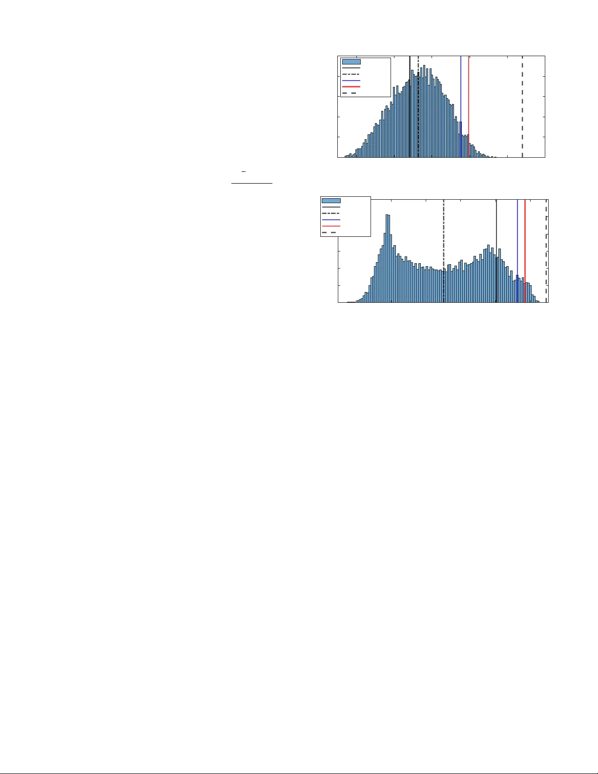
Robust H ∞ con trol under sto c hastic requiremen ts: minimizing conditional v alue-at-risk instead of w orst-case p erformance Erv an Kassarian, F rancesco Sanfedino, Daniel Alazard, Andrea Marrazza Abstract— Con v en tional robust H 2 / H ∞ con trol minimizes the w orst-case p erformance, often leading to a conserv ative design driv en by v ery rare parametric congurations. T o reduce this conserv atism while taking adv antage of the stochastic prop erties of Mon te Carlo sampling and its compatibilit y with parallel computing, w e introduce an alternativ e paradigm that optimizes the controller with resp ect to a sto chastic criterion, namely the conditional v alue at risk. W e presen t the problem form ulation and discuss several open challenges to ward a general syn thesis framew ork. The p otential of this approach is illustrated on a mechanical system, where it signican tly impro v es ov erall performance b y tolerating some degradation in v ery rare w orst-case scenarios. Index T erms— Robust H ∞ con trol, stochastic optimization, risk-a w are con trol, uncertain linear systems. I . I N T R O D U C T I O N R OBUST structured H ∞ con trol [1] traditionally aims at nding a controller that minimizes the worst-case p erformance across all p ossible parametric congurations. Denoting as T z w (s , k , δ ) a transfer function from input w to output z , which depends on the vectors k of decision v ariables and δ of uncertain parameters, this formulation reads minimize k ∈K max δ ∈D δ || T z w (s , k , δ ) || ∞ . (1) Here, K denotes the admissible space, describing the con trollers with a c hosen structure (xed-order, PID, etc.), and D δ is generally the hypercub e [ − 1 , 1] m after normalization of the m uncertain parameters. The case of a nonlinear constraint restricting D δ w as also addressed in [2]. When there are m ultiple con trol ob jectives, it is sough t to solve: minimize k ∈K max δ ∈D δ || T z 1 w 1 ( s, k , δ ) || sub ject to max 2 ≤ i ≤ n max δ ∈D δ || T z i w i ( s, k , δ ) || ≤ 1 (2) where || · || may refer to the H 2 or H ∞ system norm. The channel w 1 → z 1 corresp onds to a soft requirement to b e minimized, while the other channels w i → z i ( i > 1 ) are hard requirements, that must b e less than 1 Erv an Kassarian and Andrea Marrazza are with DYCSYT, 3 A v en ue Didier Daurat, 31400 T oulouse, F rance. F rancesco Sanfedino and Daniel Alazard are with F édération ENAC ISAE-SUP AERO ONERA, Université de T oulouse, 10 A ven ue Marc Pélegrin, T oulouse, 31400, F rance. Corresponding author’s email: erv an.kassarian@dycsyt.com (once normalized) but not necessarily minimized. As this form ulation do es not inv olve an y notion of probability , the w orst-case conguration is often extremely unlik ely , leading to a conserv ativ e design with regard to industrial requiremen ts that are generally dened in a sto chastic sense and relying on a probabilistic description of the uncertain parameters (e.g. gaussian, uniform, or other distributions). When considering deterministic parameters δ ∈ [ − 1 , 1] m , the state of the art for robust H ∞ con trol is the nonsmooth optimization algorithm of [3], implemented in MA TLAB’s function systune [4], that solv es the inner maximization problem of (1) using a lo cal search enabled b y the computation of Clarke sub dierentials [5] of the H ∞ norm [6]. Identied worst-case congurations are iterativ ely added to an active set D a ⊂ D δ on which the outer minimization problem is solved based on the algorithm of [7]. Then, global robustness verication can b e done for example with Monte Carlo sampling [8] or with µ -analysis [9]. The former provides statistical guaran tees based on the worst observ ed sample, while the latter, generally based on branch-and-bound algorithms [10], pro vides a formal guaran tee of detecting the global worst- case conguration. How ever, as noted ab ov e, this worst- case scenario can b e extremely rare, whic h motiv ated the dev elopmen t of probabilistic µ -analysis [11]. Nev ertheless, µ -based tec hniques exhibit limited scalability with the n um ber of parameters, since they rely on bounding the structured singular v alue, whose exact computation is NP-hard [12]. F urthermore, they are not oriented tow ard robust controller syn thesis, which is the primary concern of the present work. This pap er prop oses an alternativ e paradigm for robust H 2 / H ∞ con troller synthesis with tw o main ob jectives. The rst is to optimize a robust controller in the sense of stochastic requirements, b etter aligning the synthesis framew ork with the underlying uncertaint y-generating pro cess and thereby reducing conserv atism. The second is to leverage Mon te Carlo metho ds, which are commonly used in sto chastic programming [13], pro vide sto chastic guaran tees, and naturally exploit parallel computing. F or this, w e rely on the conditional v alue at risk (CV AR), a common concept in the eld of nance to quan tify p otential extreme losses in a p ortfolio. The rationale for employing CV AR ov er other risk measures, M(s) ∆ w p q z K u y Fig. 1 : LFR representation of T z w (s , k , δ ) suc h as the quantile, is tw ofold. First, it captures b oth the quantile threshold and the severit y of losses b ey ond it, providing a more complete measure of risk. Second, it is particularly suitable for optimization, as established in the literature [14]. This form ulation is in troduced in Section II, and adapted in Section I I I to b e more suitable for optimization. Section IV-A presents a rst step tow ard a solution metho d and identies several op en challenges that remain to b e addressed. Finally , Section V illustrates this metho d on the robust control of a mechanical system. I I . P R O B L E M S TA T E M E N T Considering a vector δ ∈ R m of uncertain parameters and a controller K structured by a v ector k ∈ K of decision v ariables (e.g. xed-order con troller, observer-based, PID, etc.), let us consider a transfer function T z w (s , k , δ ) under the Linear F ractional Representation (LFR) as in Fig. 1, where ∆ = diag ( δ i I n i ) ( n i is the n um ber of repetitions of δ i ). Assumption 2.1: The random v ariable δ has b ounded supp ort D δ , and its probability distribution admits a densit y p ( δ ) . Assuming a b ounded supp ort is common in control en- gineering, as it is necessary in the traditional deterministic framew ork to dene a worst case (as in Eq. (1)). In this pap er, it is necessary to realistically make Assumption 2.2 b elo w. Without loss of generality , w e consider that D δ ⊂ [ − 1 , 1] m and that δ = 0 corresp onds to the nominal conguration. F or a system norm || · || which may be the H 2 or H ∞ norm 1 in this pap er, the loss function: L z w ( k , δ ) = || T z w (s , k , δ ) || (3) is a random v ariable that dep ends on the decision vector k . Assumption 2.2: Given k ∈ K , the loss function L z w ( k , δ ) is said to satisfy Assumption 2.2 when T z w (s , k , δ ) is internally stable for all δ ∈ D δ . Assumption 2.2 ensures that the loss function is well- dened for any δ , and th us allo ws us to dene the exp ected v alue in the following. This assumption might b e seen as restrictiv e; but in practice, it can an yw a y b e desirable to guaran tee stability even in rare w orst-case scenarios, with the following sto chastic form ulation relaxing only 1 F or the H 2 norm, w e assume that the matrix D of the state- space representation is such the H 2 norm is correctly dened, cf. e.g. [15]–[17]. p z w k ( α ) α W orst case P ( || T zw (s , k , δ ) || < V AR zw β ( k )) = β CV AR zw β ( k ) V AR zw β ( k ) max δ || T zw (s , k , δ ) || Fig. 2 : Probabilit y densit y p z w k ( α ) of the loss function || T z w (s , k , δ ) || with β -V AR, β -CV AR and worst case the p erformance requirements measured with the H ∞ or H 2 norms. Assumption 2.3: Given k ∈ K , the loss function L z w ( k , δ ) is said to satisfy Assumption 2.3 when its distribution function Ψ z w ( k , α ) is contin uous. Assumption 2.3 is adopted here following the work of [14] to prop erly introduce Denition 2.4. Denition 2.4: ( β -V AR, β -CV AR) Giv en a loss function L z w ( k , δ ) satisfying Assumptions 2.1, 2.2 and 2.3, and β ∈ [0 , 1) , the β -V alue at risk ( β -V AR), noted V AR z w β ( k ) , is: V AR z w β ( k ) = min { α ∈ R : Ψ z w ( k , α ) ≥ β } . (4) The β -Conditional v alue at risk ( β -CV AR) is: CV AR z w β ( k ) = 1 1 − β Z L zw ( k,δ ) ≥ V AR zw β ( k ) L z w ( k , δ ) p ( δ ) dδ . (5) In other words, when lo oking at the probabilit y distribu- tion of the loss function L z w ( k , δ ) , V AR z w β ( k ) separates the β most fav orable cases from the (1 − β ) worst cases, while CV AR z w β ( k ) represents the conditional expected v alue of the loss associated with the w orst cases δ relativ e to that loss b eing greater than V AR z w β ( k ) . This is schematically represen ted in Fig. 2. In this pap er, we fo cus on the problem: minimize k ∈K CV AR z 1 w 1 β 1 ( k ) sub ject to CV AR z i w i β i ( k ) ≤ 1 , 2 ≤ i ≤ n (6) whic h replaces problem (2), with the main dierences: (i) the parameters δ are dened as random v ariables rather than deterministic parameters, ov er the same b ounded supp ort (Assumption 2.1), (ii) instead of minimizing the w orst case without considering any probability , we seek to minimize the conditional expected v alue of the ( 1 − β i ) w orst cases. I I I . C O M P U T A T I O N O F V A R A N D C V A R A. F ormulation as an optimization problem Denition 2.4 do es not allo w for a straightforw ard computation of the V AR and CV AR. Instead, one typ- ically relies on the following result of Ro ckafellar [14], in which b oth are c haracterized as solutions of a conv ex optimization problem. Prop osition 3.1: (Expression of β -V AR and β -CV AR as solutions of a conv ex minimization problem [14]) Under Assumptions 2.1, 2.2 and 2.3, let us dene the function F z w β ( k , α ) = α + 1 1 − β Z δ ∈ R m [ L z w ( k , δ ) − α ] + p ( δ ) dδ (7) where [ x ] + = max ( x, 0) . The β -CV AR of the loss function L z w ( k , δ ) is the minimum of F β ( k , α ) as a function of α : CV AR z w β ( k ) = min α ∈ R F z w β ( k , α ) (8) and the β -V AR is the left-end v alue of the set of all α that attain this minim um (p ossibly reducing to a single p oin t): V AR z w β ( k ) = left end p oin t of arg min α ∈ R F z w β ( k , α ) . (9) Moreo v er, F z w β ( k , α ) is con v ex and contin uously dieren- tiable as a function of α . Corollary 3.2: Optimal con troller for the β -CV AR prob- lem Problem (6) is equiv alent to: minimize k ∈K ,α ∈ R n F z 1 w 1 β 1 ( k , α 1 ) sub ject to F z i w i β i ( k , α i ) ≤ 1 , 2 ≤ i ≤ n (10) where we hav e gathered all α i in a vector α ∈ R n . B. Sample av erage appro ximation (SAA) The function F z w β ( k , α ) can b e approximated by sam- pling N i.i.d. realizations ˜ δ 1 , ˜ δ 2 , ... ˜ δ N from the densit y p and dening the sample a v erage appro ximation (SAA) [18] e F z w β ( k , α , ˜ δ ) = α + 1 (1 − β ) N N X i =1 [ L z w ( k , ˜ δ i ) − α ] + (11) that conv erges p oint-wise to F z w β ( k , α ) when N → ∞ [19]. Optimization of β -CV AR based on the SAA has b een addressed in nance-related literature [14], [20]–[22]. As an approximation of the sto chastic programming prob- lem (10), we may solv e the deterministic SAA problem: minimize k ∈K ,α ∈ R n e F z 1 w 1 β 1 ( k , α 1 , ˜ δ ) sub ject to e F z i w i β i ( k , α i , ˜ δ ) ≤ 1 , 2 ≤ i ≤ n max δ ∈D δ λ R max ( A ( k , δ )) < 0 (12) where A ( k , δ ) is the dynamics matrix of the state-space represen tation of the closed lo op, and λ R max ( · ) denotes the sp ectral abscissa. The constraint on the sp ectral abscissa ensures that Assumption 2.2 remains satised ov er the whole supp ort D δ and not only ov er the samples ˜ δ ( i ) . How this constraint can b e enforced is discussed in Section IV- A. C. Condence interv al T o obtain an accurate solution to the original problem, it is necessary to choose N sucien tly large. [23, Theorem 3] c haracterizes the conv ergence rate and derives the n um ber of samples required to guarantee a prescrib ed accuracy level with a given condence. Ho w ev er, this result also dep ends on the regularity of the uncertain loss function, which is not known a priori. In practice, thanks to the expression of V AR and CV AR as solutions of an optimization problem (Prop osition 3.1), the pro cedure prop osed in [24, Section 3.2] allo ws to assess the gap b etw een the estimated β -CV AR: \ CV AR z w β ( k ) = min α ∈ R e F z w β ( k , α , ˜ δ ) and the true one, solution of Eq. (8). Sp ecically , given a candidate solution ˆ α , one dra ws M i.i.d. batches of n v ectors ˜ δ i 1 , ˜ δ i 2 , ... ˜ δ in , i = 1 , 2 , ..., M , and dene for each batc h: G i ( n ) = 1 n n X j =1 e F z w β ( k , ˆ α, ˜ δ ij ) − min α ∈ R 1 n n X j =1 e F z w β ( k , α , ˜ δ ij ) . Since the exp ected v alue of the left and right terms are resp ectively an upp er and low er b ound of the true optim um, each G i ( n ) is an observ ation of a random v ariable G ( n ) representing the optimalit y gap. Noting ¯ G ( M , n ) = 1 M P M i =1 G i ( n ) , [24] shows that √ M ( ¯ G ( M , n ) − E ( G ( n ))) conv erges in distribution to a normal la w. Noting σ 2 G ( M , n ) the sample v ariance estimator of the v ariance of G ( n ) , and t M − 1 ,γ the (1 − γ ) -quantile of a Studen t t distribution with M − 1 degrees of freedom, then  0 , ¯ G ( M , n ) + t M − 1 ,γ σ G ( M , n ) √ M  (13) is a (1 − γ ) -interv al of condence for the optimality gap [24]. I V . O P T I M I Z A T I O N A. Optimization pro cedure Based on the formulation of previous sections, Algo- rithm 1 is proposed to tac kle the sto chastic optimization problem (6). Step 1 allows to provide an initial controller with robust stability o ver the whole supp ort, as required by Assumption 2.2. It can be p erformed with [3], which relies on the algorithm of [7] and the activ e congurations approac h describ ed in next paragraph. In [7], the pure stabilization problem is addressed with the shifted H ∞ norm [6]. Optimization of the SAA approximation is p erformed in step 2; it can b e addressed with deterministic nonsmo oth optimization, cf. section IV-B. A w orst-case searc h for unstable congurations is p erformed in step 3, as discussed in next paragraph. Finally , step 4 ev aluates the estimated CV ARs obtained with the optimized controller and their condence interv als of Section I I I-C to v alidate or inv alidate the controller. Algorithm 1 CV AR optimization Initialization: Activ e congurations D a δ = { 0 } , n umber of samples N , tolerance ϵ . Step 1: Find ˆ k 0 that robustly stabilizes T z w ( s, k , δ ) ov er the whole supp ort D δ , and up date D a δ . Step 2: F orm the SAAs with N samples, initialize k = ˆ k 0 and solv e the SAA problem (12) where robust stability o v er the whole supp ort: max δ ∈D δ λ R max ( A ( k , δ )) < 0 is replaced with stability o v er the active congurations: max δ ∈D a δ λ R max ( A ( k , δ )) < 0 . The optimal controller is noted ˆ k . Step 3: Perform worst-case searc h in stability: δ ∗ = arg max δ ∈D δ λ R max ( A ( ˆ k , δ )) . If λ R max ( A ( ˆ k , δ ∗ )) > 0 , add δ ∗ to D a δ and go back to step 2. Otherwise, go to step 4. Step 4: Ev aluate the CV ARs of problem (12), with su- cien tly tight interv als of condence. If they are dierent from those obtained in step 2 by more than ϵ %, increase N and go back to step 2. Otherwise, terminate. The identication of the global worst-case stabilit y conguration being NP-hard [12], the stabilit y o ver the whole support D δ is addressed through the active cong- urations approach of [3]. It consists of enforcing stabilit y of congurations b elonging to a subset D a δ ⊂ D δ , initialized with the nominal conguration, and up dating this subset through (deterministic) worst-case searches (step 3). This pro cedure is necessary ev en when the initial con troller stabilizes the system ov er the whole support (step 1), b ecause this property may not be main tained when solving the SAA problem (step 2). If a destabilizing conguration δ ∗ is identied in step 3, it is added to D a δ , and step 2 is repeated. Note that the step 1 t ypically also uses this approac h [3], and thus, it also up dates D a δ . B. Op en challenges While w e ha v e prop osed a general metho d to address the CV AR optimization, there are still op en challenges to address the form ulated problem in a systematic and ecien t wa y . F uture researc h should fo cus on dev eloping suitable nonsmo oth algorithms to address step 2 of Algorithm 1, ecien tly and with con v ergence certicates. Of particular in terest is the w ork of [25], which prop oses an algorithm that tolerates inexact computation of the gradient or of the function itself. This algorithm is sp ecically designed for low er- C 1 functions, a class to whic h the SAA e F z w β ( k , α ) can easily be shown to belong under Assumptions 2.1, 2.2 and 2.3, since this prop erty holds for || T z w ( s, k , δ ) || ∞ as a function of k as long as T z w ( s, k , δ ) is internally stable [3, Prop osition 2]. In particular, [25] illustrates their metho d on the H ∞ norm where the exactness of the computation, based on a dichotom y inv olving the b ounded real lemma, can b e relaxed. This property is particularly desirable in our SAA where we ha v e to ev aluate many times the H ∞ norm, and where our SAA is itself an approximation. Imp ortance sampling [18], [26] is a technique used in rare even t simulation that can reduce the v ariance of the SAA and reduce the required num b er of samples. It may particularly b e useful when c hoosing a β v ery close to 1. F or example, it was applied to CV AR in [20], [21], [27]. Performing imp ortance sampling in a context of optimization is challenging, since an appropriate sampling distribution may dep end on k and therefore has to b e up dated during optimization [20], [26]. Finally , in this pap er, the distributions are assumed to be p erfectly known. When this assumption do es not hold, distributionally robust control provides a natural extension; see, for example, [28], [29]. V . A P P L I C A T I O N A. Benchmark W e consider the b enchmark of [2], namely the attitude con trol of a exible spacecraft G ( s, δ ) to follow a refer- ence r . The closed loop is represented in Fig. 3, where d ( s ) represen ts actuator dynamics. The control input u of the plan t is the torque (3 comp onen ts) applied to the satellite and the output v ector contains the 3 angle measurements p olluted b y some noise n . W e note k ∈ K the decision v ariables describing the controllers K ( s ) of the desired structure: one 4-th order controller p er spacecraft axis, eac h one taking the measured angle and rate as inputs and generating a control torque. The closed-lo op system has 50 states, 43 uncertain parameters δ i , and 72 decision parameters k i . G (s , δ ) K (s) e r s n u d (s) Fig. 3 : Benchmark: closed-lo op system The uncertain parameters represent mechanical prop er- ties. Once normalized, they all follow a Gaussian distri- bution of mean 0 and standard deviation 1 / 3 , truncated at 3 σ , except for one parameter (representing an angle) whic h follo ws a uniform distribution b etw een -1 and 1. A dditionally , the vectors δ that do not satisfy a nonlinear constrain t c ( δ ) ≤ 0 , related to some mechanical constrain t detailed in [2], m ust b e remo ved from the robustness analysis. In the deterministic setting, this constraint can b e addressed in the framew ork of constrained optimization as in [2]. In the β -CV AR form ulation, when p erforming Mon te Carlo sampling, samples that do not satisfy the constrain t are simply discarded; all follo wing results ( β - V AR, β -CV AR, mean, distribution) refer to the resulting conditional distribution. The con trol problem consists in robustly placing a con trol bandwidth of 0.1 rad/s (Req. 3) while ensuring a mo dulus margin of 0.5 (Req. 2) and minimizing the v ariance of the actuator command in resp onse to mea- suremen t noise (Req. 1). It in volv es the 3 loss functions: L un ( s, k , δ ) = || W 1 T n → u ( s, K , δ ) || 2 2 L us ( s, k , δ ) = || W 2 T s → u ( s, K , δ ) || ∞ L er ( s, k , δ ) = || W 3 ( s ) T r → e ( s, K , δ ) || ∞ with W 1 a normalization constan t, W 2 = 1 2 to ensure the desired mo dulus margin, W 3 ( s ) = 10s+1 2(10s+0 . 01) I 3 a w eigh ting lter to imp ose the desired bandwidth. Next sec- tions detail the corresponding deterministic and sto chastic form ulations. B. F ormulation as a deterministic control problem In the deterministic form ulation, the space of (deter- ministic) uncertain parameters is the support of δ : D δ = { δ ∈ [ − 1 , 1] m suc h that c ( δ ) ≤ 0 } without any consideration of probabilit y . Under the tra- ditional robust control framework, the control problem reads: minimize K ∈K max δ ∈D δ L un ( s, k , δ ) (Req. 1) sub ject to max δ ∈D δ L us ( s, k , δ ) ≤ 1 (Req. 2) max δ ∈D δ L er ( s, k , δ ) ≤ 1 (Req. 3) and is solv ed with the metho d of [2]. Let us note ˆ k det the decision parameters describing the optimal controller. The resulting densities for L un ( s, ˆ k det , δ ) (Req. 1, Fig 4a) and L us ( s, ˆ k det , δ ) (Req. 2, Fig 4b) are presented in Fig. 4 using 10000 samples. It can b e v eried that the w orst case for Req. 2, computed with the deterministic metho d of [2], is indeed less than 1, as imp osed. The mean, β -V aR and β -CV aR ( β = 95%) are reported even though they w ere not used when solving the optimization problem. Nominal p erformance, i.e. when δ = 0 , is also indicated for completeness. All p erformance metrics are summarized in T able I, including Req. 3, whic h is not represented in the gures. C. F ormulation as a sto chastic control problem Based on the notations of Denition 3.1, w e x β = 95 % and seek to solve the sto chastic problem: minimize K ∈K CV AR un β ( k ) (Req. 1) sub ject to CV AR us β ( k ) ≤ 1 (Req. 2) CV AR er β ( k ) ≤ 1 (Req. 3) whic h we replace, for a set ˜ δ of i.i.d. realizations, by the deterministic problem: minimize K ∈K , α ∈ R 3 e F un β ( k , α 1 , ˜ δ ) (Req. 1) sub ject to e F us β ( k , α 2 , ˜ δ ) ≤ 1 (Req. 2) e F er β ( k , α 3 , ˜ δ ) ≤ 1 (Req. 3) max δ ∈D δ λ R max ( A ( k , δ )) < 0 , 0.9 5 1 1.0 5 1.1 1 .15 1 .2 p ^ k det ( , ) 0 0.0 05 0.0 1 0.0 15 0.0 2 0.0 25 Histogram Nominal Me an V AR CV AR Worst-case (a) Densit y of L un ( s, ˆ k det , δ ) (Req. 1) , 0.8 2 0.8 4 0.8 6 0.8 8 0.9 0 .92 p ^ k det ( , ) 0 0.0 05 0.0 1 0.0 15 0 . 0 2 0 . 0 2 5 0 . 0 3 Histogram Nominal Me an V AR CV AR Worst-case (b) Densit y of L us ( s, ˆ k det , δ ) (Req. 2) Fig. 4 : Empirical probability densities with solution ˆ k det W e solv ed this problem with Algorithm 1, using ˆ k det as initial con troller (step 1). Step 2 was performed with MA TLAB’s function fmincon [30] using the sequen tial quadratic programming (SQP) algorithm, ev en though con v ergence to an optim um is not formally guaran teed due to the nonsmo othness of the SAA. The constraint on the sp ectral abscissa was not explicitly taken into account when solving Step 2, but stability ov er the whole domain w as v eried a p osteriori in Step 3 using the metho d of [2] (note that Req. 2, b y imp osing a constraint on the CV AR of the stability margins, helps enforce stability). 2500 samples w ere used initially in the SAAs, and this num ber w as increased to 10000 following step 4. With these 10000 samples, the 99% condence interv al of Eq. (13) w as at most 0 . 0008 among the 3 requirements, which w as considered sucien t for v alidation. W e note ˆ k sto the decision parameters describing the optimal con troller. T o compare with the results of the deterministic form u- lation of Section V-B, we also computed the worst case with the method of [2], although this computation was not p erformed during the optimization itself. The results are presented in Fig. 5 and summarized in T able I. In particular: 1) Fig. 5b: The β -CV AR of L us ( s, ˆ k sto , δ ) (Req. 2) is 0.98, whic h is less than 1 as imp osed. A worst-case of 2.05 (again found with the deterministic metho d of [2]) is tolerated, whereas it w ould hav e b een rejected with the traditional form ulation. Nev ertheless, this worst case is v ery rare. T o illustrate this statement, we also mention that among the 10,000 samples used to construct the histogram, the maxim um observed v alue was 1.58. This implies, with 99.99% condence, that at least 99.9% of the underlying distribution lies b elow 1.58. 2 2) Fig. 5a: As a result of relaxing Req. 2 (from worst case to CV AR criterion), the Req. 1 is considerably improv ed: all metrics were reduced b y ∼ 30% with resp ect to Section V- B. , 0.65 0.7 0.75 0.8 p ^ k sto ( , ) 0 0.005 0.01 0.015 0.02 0.025 0.03 Histogram Nominal Mean V AR CV A R Wo rst-ca se (a) Densit y of L un ( s, ˆ k sto , δ ) (Req. 1) , 0.8 1 1.2 1.4 1.6 1.8 2 2.2 p ^ k sto ( , ) 0 0.002 0.004 0.006 0.008 0.01 0.012 Histogram Nominal Mean V AR CV A R Worst-ca se (b) Densit y of L us ( s, ˆ k sto , δ ) (Req. 2) Fig. 5 : Empirical probability densities with solution ˆ k sto T ABLE I : P erformance metrics for the deterministic (det.) and sto chastic (sto.) approaches. Req.1 Nominal Mean β -V AR β -CV AR W orst det. 1.02 1.03 1.09 1.10 1.17 sto. 0.69 0.70 0.73 0.74 0.79 Req.2 det. 0.90 0.87 0.91 0.92 0.93 sto. 0.87 0.79 0.87 0.98 2.05 Req.3 det. 1.00 1.00 1.00 1.00 1.00 sto. 1.00 1.00 1.00 1.00 1.05 2 F or a random function f ( δ ) , noting δ ∗ the sample realizing the largest function evaluation, [8] shows that P(P( f ( δ ) > f ( δ ∗ )) ≤ ϵ ) ≥ 1 − γ is guaranteed when N v eries: N > ln ( γ ) ln (1 − ϵ ) . V I . C O N C L U S I O N T o reduce the conserv atism of conv entional robust H ∞ con trol, which minimizes a worst-case performance that may b e very unlikely , we introduced an alternative sto chastic approach based on the conditional v alue at risk. Its capacity to signican tly improv e the performance of uncertain control systems, at the exp ense of tolerating rare degrading worst-case congurations, was illustrated on a mechanical system. Finally , we presented a rst step to ward a syn thesis metho d and highligh ted sev eral remaining op en challenges. R E F E R E N C E S [1] P . Apkarian and D. Noll, “The H innity Con trol Problem is Solved,” Aerospace Lab, no. 13, pp. 1–27, 2017. [2] E. Kassarian, F. Sanfedino, D. Alazard, and A. Marrazza, “W orst-case search in constrained uncertaint y space for robust H-innity syn thesis,” Nov. 2025, arXiv:2511.15480 [eess]. [Online]. A v ailable: [3] P . Apkarian, M. N. Dao, and D. Noll, “Parametric Robust Structured Control Design,” IEEE T ransactions on Automatic Control, vol. 60, no. 7, pp. 1857–1869, 2015, arXiv: 1405.4202. [4] “Systune, Matlab help page. ” [Online]. A v ailable: https://fr.math works.com/help/con trol/ref/dynamicsystem.systune.html [5] F. Clark e, Optimization and nonsmo oth analysis. Society for industrial and Applied Mathematics, 1990. [6] S. Boyd and C. Barratt, Linear Controller Design: Limits of Performance. Englewoo d Clis, NJ: Prentice Hall., 1991. [7] P . Apkarian and D. Noll, “Nonsmooth H innity synthesis,” IEEE T ransactions on Automatic Con trol, vol. 51, no. 1, pp. 71–86, 2006. [8] R. T emp o, E. Bai, and F. Dabb ene, “Probabilistic robustness analysis: explicit bounds for the minimum num b er of samples,” in Proceedings of 35th IEEE Conference on Decision and Control, vol. 3. K obe, Japan: IEEE, 1996, pp. 3424–3428. [Online]. A v ailable: http://ieeexplore.ieee.org/document/573690/ [9] J. Doyle, “Analysis of feedback systems with structured uncer- tainties,” IEE Pro ceedings D Control Theory and Applications, vol. 129, no. 6, p. 242, 1982. [Online]. A v ailable: https://digital- library .theiet.org/conten t/journals/10.1049/ip-d.1982.0053 [10] C. Roos, “Systems modeling, analysis and control (SMAC) to olbox: An insight into the robustness analysis library ,” in 2013 IEEE Conference on Computer Aided Control System Design (CA CSD). Hyderabad, India: IEEE, Aug. 2013, pp. 176–181. [Online]. A v ailable: http://ieeexplore.ieee.org/document/6663479/ [11] J.-M. Biannic, C. Ro os, S. Bennani, F. Bo quet, V. Preda, and B. Girouart, “A dv anced probabilistic m u -analysis techniques for AOCS v alidation,” Europ ean Journal of Control, vol. 62, pp. 120–129, Nov. 2021. [Online]. A v ailable: https://linkingh ub.elsevier.com/retrieve/pii/S0947358021000789 [12] O. T oker and H. Ozbay , “On the complexity of purely complex mu computation and related problems in multidimensional systems,” IEEE T ransactions on Automatic Control, v ol. 43, no. 3, pp. 409–414, Mar. 1998. [13] A. Shapiro, D. Den tc hev a, and A. R uszczyński, Lectures on Stochastic Programming: Modeling and Theory . So ciety for Industrial and Applied Mathematics, Jan. 2009. [14] R. T. Ro ckafellar and S. Ury asev, “Optimization of conditional v alue-at-risk,” The Journal of Risk, vol. 2, no. 3, pp. 21–41, 2000. [15] T. Rautert and E. W. Sac hs, “Computational Design of Optimal Output F eedback Controllers,” SIAM Journal on Optimization, vol. 7, no. 3, pp. 837–852, Aug. 1997. [16] P . Apkarian, D. Noll, and A. Rondepierre, “Mixed H2/Hinnity control via nonsmo oth optimization,” in Pro ceedings of the 48h IEEE Conference on Decision and Control (CDC) held jointly with 2009 28th Chinese Control Conference. Shanghai, China: IEEE, Dec. 2009, pp. 6460–6465. [17] D. Arzelier, D. Georgia, S. Gumusso y , and D. Henrion, “H2 for HIFOO,” in In ternational Conference on Control and Op- timization With Industrial Applications (COIA 2011), Ankara, T urkey , 2011. [18] T. Homem-de Mello and G. Bayraksan, “Monte Carlo sampling- based metho ds for sto chastic optimization,” Surveys in Op er- ations Research and Management Science, vol. 19, no. 1, pp. 56–85, Jan. 2014. [19] A. Shapiro, “Monte Carlo sampling approach to sto chastic programming,” ESAIM: Pro ceedings, vol. 13, pp. 65–73, Dec. 2003. [20] O. Bardou, N. F rikha, and G. Pagès, “Computing V aR and CV aR using sto chastic approximation and adaptiv e uncon- strained imp ortance sampling,” Monte Carlo Metho ds and Applications, vol. 15, no. 3, Jan. 2009. [21] A. T amar, Y. Glassner, and S. Mannor, “Optimizing the CV aR via Sampling,” Pro ceedings of the AAAI Conference on Arti- cial Intelligence, vol. 29, no. 1, F eb. 2015. [22] Y. T akano, K. Nanjo, N. Sukegaw a, and S. Mizuno, “Cutting plane algorithms for mean-CV aR p ortfolio optimization with nonconv ex transaction costs,” Computational Management Sci- ence, vol. 12, no. 2, pp. 319–340, Apr. 2015. [23] A. Cherukuri, “Sample av erage approximation of conditional v alue-at-risk based v ariational inequalities,” Optimization Let- ters, vol. 18, no. 2, pp. 471–496, Mar. 2024. [24] W.-K. Mak, D. P . Morton, and R. W oo d, “Mon te Carlo b ound- ing techniques for determining solution quality in sto chastic programs,” Op erations Research Letters, vol. 24, no. 1-2, pp. 47–56, F eb. 1999. [25] D. Noll, “Bundle Metho d for Non-Conv ex Minimization with Inexact Subgradients and F unction V alues,” in Computational and Analytical Mathematics, vol. 50. New Y ork, NY: Springer New Y ork, 2013, pp. 555–592, series Title: Springer Pro ceedings in Mathematics & Statistics. [26] L. Aolaritei, B. P . G. V. P arys, H. Lam, and M. I. Jordan, “Stochastic Optimization with Optimal Imp ortance Sampling,” Apr. 2025, arXiv:2504.03560 [math]. [27] L. Sun and L. J. Hong, “A general framework of imp ortance sampling for value-at-risk and conditional v alue-at-risk,” in Proceedings of the 2009 Winter Simulation Conference (WSC). Austin, TX, USA: IEEE, Dec. 2009, pp. 415–422. [28] B. V an Parys, D. Kuhn, P . Goulart, and M. Morari, “Distri- butionally Robust Control of Constrained Sto chastic Systems,” IEEE T ransactions on Automatic Control, pp. 1–1, 2015. [29] A. Hakob yan and I. Y ang, “W asserstein Distributionally Ro- bust Motion Control for Collision A voidance Using Conditional V alue-at-Risk,” IEEE T ransactions on Rob otics, vol. 38, no. 2, pp. 939–957, Apr. 2022. [30] “Constrained Nonlinear Optimization Algorithms, Matlab help page,” 2025. [Online]. A v ail- able: https://fr.math works.com/help/optim/ug/constrained- nonlinear-optimization-algorithms.html