Estimation in moderately misspecified models

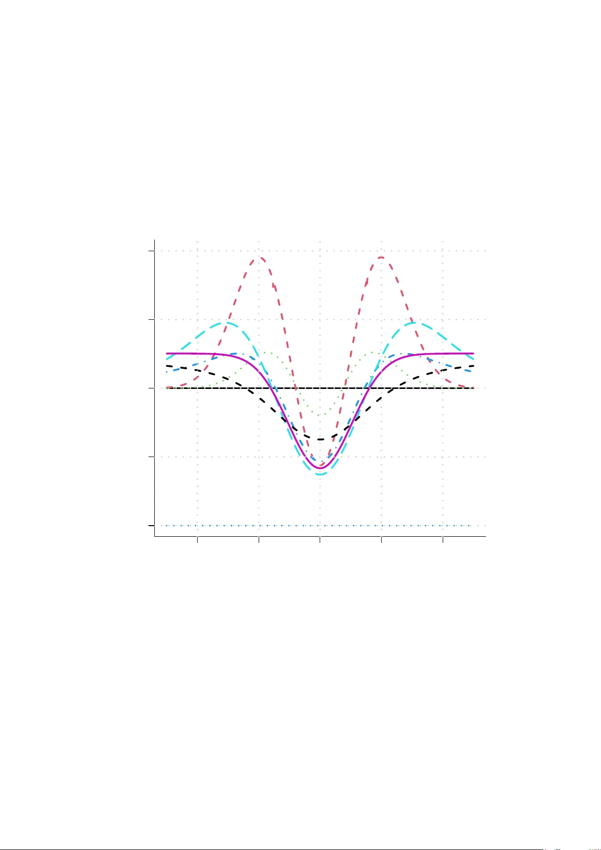
Estimation in mo derately missp eciﬁed mo dels Nils Lid Hjort Univ ersit y of Oslo and Univ ersit y of Oxford Abstra ct . Supp ose data are ﬁtted to some parametric model but that the true mo del happ ens to b e one with an additional parameter. When a parameter is to b e estimated one can use likelihoo d estimation in the wider mo del or in the narro w mo del. Including the extra parameter in the mo del means less bias but larger sampling v ariabilit y . Tw o basic questions are addressed in this article. (i) Just ho w muc h missp eciﬁcation can the narro w mo del tolerate? In the con text of a large-sample mo derate misspeciﬁcation framew ork w e ﬁnd a surprisingly simple, sharp, and general answ er. There is eﬀectiv ely a ‘tolerance radius’ around a giv en narro w mo del, inside of which narrow es timation is more precise than wide estimation for all estimands. This is computed in a selection of examples that also demonstrate the degree of robustness of imp ortan t standard metho ds against mo derate incorrectness of the mo del under whic h they are optimal. (ii) Are there other estimators that work w ell b oth under narro w and wide circumstances? W e discuss several p ossibilities and prop ose some new pro cedures. All metho ds are compared in a broad large-sample p erformance study . Key words: Ak aike criterion, compromise estimators, delib erate bias, missp ec- iﬁed model, parametric inference, tolerance radius 1. In tro duction and motiv ating examples. Our theme is mo derately missp ec- iﬁed parametric mo dels, and w e ask t w o main questions. The ﬁrst is: Just ho w muc h missp eciﬁcation can a giv en parametric mo del tolerate in a certain direction? More sp ecif- ically , when is it adv antageous to stick to the narro w mo del, even when it is incorrect? When will ‘narro w estimation’ b e more precise than ‘wide estimation’ ? The second ques- tion is broader: Are there estimators that are ab out as go o d as the narro w estimator when the narrow mo del is correct, and ab out as go od as the wide estimator when the narrow mo del is incorrect? W e shall presen t a generous list of examples to motiv ate the problems and precise form ulations of them. Example A. Supp ose data Y 1 , . . . , Y n come from a life distribution on [0 , ∞ ) and that the median µ is to b e estimated. If the density is the exponential f ( y ) = θ e − θ y , then µ = log 2 /θ , and a natural estimator is b µ narr = log 2 / b θ narr , where b θ narr = 1 / ¯ Y is the maximum lik elihoo d (ML) estimator in this narro w mo del. If it is susp ected that the mo del could deviate from simple exp onen tialit y in direction of the W eibull distribution, with f ( y , θ , γ ) = exp {− ( θ y ) γ } γ ( θ y ) γ − 1 θ , y > 0 , (1 . 1) then w e should conceiv ably use b µ wide = (log 2) 1 / b γ / b θ , using ML estimators b θ , b γ in the wider W eibull mo del. But if the simple mo del is righ t, i.e. γ = 1, then b µ narr is b etter, in terms (for example) of mean squared error. By sheer contin uity it should b e b etter also for γ ’s close to 1. Ho w muc h must γ diﬀer from 1 in order for b µ wide to b ecome b etter? And what Nils Lid Hjort 1 Ma y 1993 with similar questions for other t ypical parametric departures from exp onen tialit y , like the gamma family? Example B. The most p opular mo delling of data Y 1 , . . . , Y n is to p ostulate normalit y , i.e. assuming f ( y ) = φ (( y − ξ ) /σ ) /σ for suitable parameters ξ and σ . In man y situations the normal density is to o light-tailed to constitute a serious description, how ever. A remedy then is to use f ( y , ξ , σ, m ) = g m  y − ξ σ  1 σ , where g m ( t ) is the t -density with m degrees of freedom. The narrow er normal mo del corresp onds to m = ∞ , and it is naturally felt that for large m the discrepancy b etw een normalit y and t -ness shouldn’t matter. Supp ose for example that the parameter to be estimated is sd, the standard deviation for Y i ’s. F or how large m is it the case that the narro w-mo del estimator b sd narr , whic h happ ens to b e the ordinary empirical standard deviation, is b etter than the more lab orious b sd wide = r b m b m − 2 b σ , computed from ML estimates b ξ , b σ , b m in the three-parameter mo del? What with other parameters to estimate than the standard deviation? Example C. Consider a regression situation with n pairs ( x i , Y i ). The classical model sa ys Y i ∼ N { α + β x i , σ 2 } for appropriate parameters α , β , σ , and encourages for example b µ narr = b α narr + b β narr x as the es timator for the median (or mean v alue) of the distribution of Y for a giv en x v alue. Supp ose how ev er that the regression curv e could b e mo derately quadratic, say Y i ∼ N { α + β x i + γ ( x i − ¯ x ) 2 , σ 2 } for a mo derate γ . Ho w m uc h m ust γ diﬀer from zero in order for b µ wide = b α + b β x + b γ ( x − ¯ x ) 2 , with regression parameters now ev aluated in the wider model, to p erform b etter? The same questions could b e asked for other parameters, like comparing b x 0 , narr with b x 0 , wide , the narrow-model based and the wide-mo del based estimators of the p oin t x 0 at which the regression curv e crosses a certain level. And ﬁnally similar questions could b e discussed in the framew ork of am omitted co v ariate. Example D. In some situations a more interesting departure from standard regression lies in v ariance heterogeneit y . This could for example suggest using Y i ∼ N { α + β x i , σ 2 (1 + γ x i ) } , where γ is zero under classical regression. F or what range of γ v alues are standard metho ds, all deriv ed under the γ = 0 hypothesis, still b etter than four-parameter-mo del analysis? Example E. Let us also include another type of mo del uncertain t y , that of missp eci- ﬁcation due to using an incorrect transformation. The transformation mo del in v en ted here Mo derately missp eciﬁed mo dels 2 Ma y 1993 has some of the in ten tions of the Box–Co x pow er transformation sc heme, but a v oids some of its pitfalls. It postulates that h λ  ( Y i − α − β x i ) /σ  ∼ N { 0 , 1 } , where h λ ( z ) = Φ − 1 { Φ( z ) λ } , (1 . 2) for appropriate v alues of ( α, β , σ, λ ); λ = λ 0 = 1 brings us back to classics. Let us brieﬂy discuss this mo del and its use b efore w e concen trate on the local missp eciﬁcation part. It can b e written Y i = α + β x i + σ Z i , where h λ ( Z i ) follows the standard normal distribution for suitable transformation parameter. V arying λ gives a fair range of transformations, and in particular includes the p ossibilit y of having sk ew ed error distributions. The four parameters can b e estimated from the data. The notation is p ossibly deceiving in that it in vites one to think in terms of ‘ α + β x i plus noise with lev el σ ’. This is not quite the case since Z i has a sk ew ed distribution with mean and median diﬀerent from zero. It is advisable to reparameterise, after ha ving found a suitable λ from data, to the familiar structure + noise form. One p ossibilit y is Y i = { α + σ e ( λ ) } + β x i + σv ( λ ) Z 0 i , in whic h e ( λ ) and v ( λ ) are mean v alue and standard deviation of Z i , under the h λ ( Z i ) ∼ N { 0 , 1 } mo del, and where Z 0 i no w has mean zero and standard deviation 1. Another p ossibilit y is Y i = { α + σ Φ − 1 (0 . 50 1 /λ ) } + β x i + σ { Φ − 1 (0 . 75 1 /λ ) − Φ − 1 (0 . 25 1 /λ ) } Z 0 i = α 0 + β x i + σ 0 Z 0 i , (1 . 3) the p oin t being that Z 0 i has median zero and in terquartile range 1. Our technical p oin t is that (1.2) is a useful generalisation of classical regression to situations with skew ed errors, and that parameter estimation is p erhaps b est carried out using ML mac hinery on (1.2); and our statistical p oint is that (1.3) b etter con v eys the structure and the noise in the data, and should b e used p ost estimation. The presen t concern is how robust standard metho ds, whic h presume λ = 1, are against missp eciﬁcation of that parameter. Should one use b µ wide ( x ) = b α wide + b β wide x + b σ wide Φ − 1 (0 . 50 1 / b λ wide ) (1 . 4) to estimate the median of Y for given x , or will the eﬀortlessly obtainable b µ narr ( x ) = b α narr + b β narr x suﬃce? Example F. Next consider logistic regression, in whic h pairs ( x i , Y i ) are observ ed of the t yp e Y i | x i ∼ Bin { 1 , p ( x i ) } , with p ( x ) = exp( α + β x ) / { 1 + exp( α + β x ) } b eing the standard mo del. Again we can ask whether standard metho ds based on ( b α narr , b β narr ), for example for estimating the true p ( x ) at a given x , or for estimating the cut-oﬀ p oint at whic h p ( x ) exceeds 1 2 , b ecome seriously inferior under mo derate missp eciﬁcations. One natural t ype of departure is mo delled b y adding a quadratic term γ ( x i − ¯ x ) 2 to the linear term; another is p ( x ) = p ( x, α , β , η ) = n exp( α + β x ) 1 + exp( α + β x ) o η , (1 . 5) Nils Lid Hjort 3 Ma y 1993 where it is of in terest to v ary η around η 0 = 1. Example G. Our ﬁnal example is the t w o-sample mo del with v ariances that may or ma y not b e equal. So X 1 , . . . , X m are N { ξ 1 , σ 2 1 } and Y 1 , . . . , Y n are N { ξ 2 , σ 2 2 } , all of them are indep enden t, and the narrow mo del sp eciﬁes that σ 1 = σ 2 . Under this assumption it is easy to put up estimators, conﬁdence interv als etc. for parameters related to the diﬀerence b et w een the X -distribution and the Y -distribution, lik e the Mahalanobis distance ∆ = | ξ 2 − ξ 1 | /σ . More awkw ard methods are needed when σ 2 6 = σ 1 , cf. the Behrens–Fisher problem. The in some sense natural generalisation of the Mahalanobis distance is for example ∆ = ( ν 2 + ω 2 ) 1 / 2 , where ν 2 = ( ξ 2 − ξ 1 ) 2 /σ 2 , ω 2 = 4 log σ 2 σ 1 σ 2 , σ 2 = ( σ 2 1 + σ 2 2 ) / 2 , see Hjort (1986a, Ch. 10). Ho w resistan t is the simple b ∆ narr = | ¯ Y − ¯ X | / b σ narr to diﬀerences in σ 1 , σ 2 ? When is it necessary to use the m uc h more complicated b ∆ wide ? Let us summarise the common characteristics of these situations. There is a narrow and usually simple parametric mo del which can b e ﬁtted to the data, but there is a p oten tial missp eciﬁcation, which can b e ameliorated by its encapsulation in a wider mo del with one additional parameter. Estimating a parameter assuming correctness of the narrow mo del in v olv es mo delling bias, but doing it in the wider mo del could mean larger sampling v ariabilit y . Th us the c hoice of metho d b ecomes a statistical balancing act with p erhaps delib erate bias against v ariance. The examples ab o v e span a reasonable range of hea vily used ‘narrow’ mo dels along with indications of rather typical kinds of deviances from them. Many standard textb o ok metho ds for parametric inference are derived under the conditions of suc h narro w mo dels. Our main result, deriv ed in Section 3, is a surprisingly sharp and general large-sample criterion for ho w m uc h missp eciﬁcation a giv en narro w mo del can tolerate. This criterion is applied to Examples A–G in Section 7. It is relatively easy to compute, in that it only in v olv es the familiar Fisher information matrix, for the wide mo del, but ev aluated under narro w mo del conditions. A particular facet of our tolerance criterion is that it do es not dep end upon the particular parameter estimand at all. In addition to quantifying the degree of robustness of standard metho ds there are also pragmatic reasons for the present inv estigation. Statistical analysis will in practice still b e carried out using narro w mo del based metho ds in the ma jority of cases, for reasons of ignorance, simplicity , na ¨ ıvit ´ e and b oldness; using wide mo del metho ds will v ery often b e muc h more lab orious, and only exp erts will use them an yho w. Thus it is of interest to quan tify the consequences of ignorance, and it would b e nice to obtain p ermission to go on doing analysis as if the simple mo del w ere true. Such a partial permission is in fact giv en here. The results of this pap er can b e in terpreted as sa ying that ‘ignorance is (sometimes) strength)’; mild departures from the narro w mo del do not really matter, and more ambitious metho ds could p erform worse. In the examples of Section 7 quite Mo derately missp eciﬁed mo dels 4 Ma y 1993 explicit limits are giv en for the degree of missp eciﬁcation that is tolerable. This upp er limit is in most cases dep enden t up on parameters of the mo del, and should b e estimated b y the conscientious statistician in situations where departures of the t yp e describ ed are susp ected. The compromise estimators that w e adv ocate in Section 5 utilise this departure estimate. Sev eral tangen tial topics are tak en up in Section 4. These include measures of distance from null mo del to the least tolerable missp eciﬁcation; comparison with the mo del selection criteria of Ak aike and Sch w arz; sim ulation based ev aluation of our criterion; discussion of the concept of a robust mo del; dangerous v ersus noncritical departures from a mo del; and in terpretation of conﬁdence in terv als under missp eciﬁcation. Deviances from a mo del in more than one direction is brieﬂy discussed at the end of Section 5. There is also ro om for impro v emen t o v er the narrow and wide metho ds. In Section 5 some new estimators are prop osed that are designed to work well b oth under narro w and wide circumstances. A broad comparison of the v arious compromise estimators is made, in a large-sample framew ork of mo derately missp eciﬁed parametric mo dels. A connection to Ba yesian robustness is also made. W e are able to make a quite general and drastic reduction: The p erformance of a large class of competing estimators can b e studied in a m uc h simpler and v ery classical con text, that of estimating a in a N { a, 1 } situation with one observ ation! Here the narrow mo del corresp onds to a = 0. This provides fresh motiv ation for studying a -estimators that in v arious wa ys tak e into account that v alues of a in the vicinity of zero are p erhaps more lik ely or p erhaps more imp ortan t. Suc h a study is rep orted on in Sections 5 and 6. The traditional robustness literature is mostly concerned with construction of meth- o ds that p erform well o v er a ‘nonparametric neigh b ourhoo d’ around some basic mo del. The presen t work is diﬀerent in that it envisages sp eciﬁc, parametric alternatives to the basic mo del. There is a literature on parametric robustness, perhaps c hieﬂy concerned with studying b eha viour of standard metho ds and modiﬁed standard metho ds under natural vi- olations of the basic mo del. Only rarely ha ve comparisons been made b etw een ‘narro w’ and ‘wide’ metho ds, how ever. Some pap ers ha v e calculated and commen ted on the increased estimation noise for a narro w mo del parameter when passing to a wider model, lik e compar- ing the v ariances of b θ narr and b θ wide in Example A. This is b eside the point, partly confusing, and not very in teresting, since what matters is studying ‘real’ parameters whic h are mean- ingful functions of the full model, as the median µ = µ ( f ) = µ ( θ , γ ) = (log 2) 1 /γ /θ in Example A, the standard deviation sd = sd( f ) = st( ξ , σ, m ) = { m/ ( m − 2) } 1 / 2 σ in Exam- ple B, etcetera. Bic k el (1984) is on the other hand clear about this issue, and is concerned with sev eral problems that resem ble those considered here. He do es not compare narrow and wide metho ds, and do es not study tolerance distances, but works directly with certain minimax strategies, in a framew ork of nested linear normal mo dels; see also 5G b elo w. The pap er by Berger (1982) on Ba y esian robustness also turns out to b e related to some of these questions. See Bic k el’s commen ts on Berger and 5E, 5F, 5G below. Nils Lid Hjort 5 Ma y 1993 2. Large-sample framework for the problem. W e shall start our inv estigation in the i.i.d. framew ork. Supp ose Y 1 , . . . , Y n come from some common density f , and represen t the wide mo del as f ( y ) = f ( y , θ , γ ), where γ = γ 0 corresp onds to the narro w mo del, say f ( y , θ ) = f ( y , θ , γ 0 ). W e assume that θ = ( θ 1 , . . . , θ p ) 0 lies in some op en region in Euclidean p -space, that γ lies in some op en in terv al containing γ 0 , and that the wide mo del is ‘smooth’; for deﬁniteness we p ostulate that the regularity conditions put forward in Lehmann’s (1983) c hapter 6.4 are in force. W e are to study b eha viour of estimators when γ deviates from γ 0 . The parameter to be estimated is some µ = µ ( f ), whic h w e write as µ ( θ , γ ) since the wider mo del is assumed to b e an adequate description of realit y . W e concen trate on ML pro cedures, and write b θ narr for the estimator of θ in the narro w model and ( b θ , b γ ) for the estimators in the wide mo del. The t w o ma jor en tries in the comp etition are b µ narr = µ ( b θ narr , γ 0 ) and b µ wide = µ ( b θ , b γ ) (2 . 1) (but see Section 5 for other estimators). These could b e compared in an asymptotic framew ork in which Y i ’s come from some ﬁxed f ( y , θ 0 , γ ), and γ 6 = γ 0 . In this case √ n ( b µ wide − µ ) has a limit distribution, whic h can b e deriv ed from the prop osition b elo w. The situation is diﬀerent for the narro w mo del pro cedure. Here √ n ( b µ narr − µ ) can be represen ted as a sum of tw o terms. The ﬁrst is √ n { µ ( b θ narr , γ 0 ) − µ ( θ 0 , γ 0 ) } , which has a limit distribution, with generally smaller v ariabilit y than that of the wide mo del pro cedure, and the second is − √ n { µ ( θ 0 , γ ) − µ ( θ 0 , γ 0 ) } , whic h tends to plus or minus inﬁnit y , reﬂecting a bias that for very large n will dominate completely . This merely go es to show that with very large sample sizes one is penalised for any bias and one should use the wide model. This result is not v ery informative, how ever, and suggests that a large-sample framework which uses a lo cal neigh b ourhoo d of γ 0 that shrinks when the sample size gro ws is m uc h more adequate. Study therefore mo del P n , the n ’th mo del, under which Y 1 , . . . , Y n are i . i . d . from f n ( y ) = f ( y , θ 0 , γ 0 + δ / √ n ) , (2 . 2) and where θ 0 is ﬁxed but arbitrary . In this framework w e need limit distributions for the wide mo del estimators ( b θ , b γ ) and for the narro w mo del estimator b θ narr . Consider  U ( y ) V ( y )  =  ∂ log f ( y , θ 0 , γ 0 ) /∂ θ ∂ log f ( y , θ 0 , γ 0 ) /∂ γ  , (2 . 3) the score function for the wide mo del, but ev aluated at the null p oin t ( θ 0 , γ 0 ). The accom- pan ying familiar ( p + 1) × ( p + 1) size information matrix is J wide = V AR 0  ∂ log f ( Y , θ 0 , γ 0 ) /∂ θ ∂ log f ( Y , θ 0 , γ 0 ) /∂ γ  =  J 11 J 12 J 21 J 22  . Note that the p × p size J 11 is simply the information matrix of the narro w mo del, ev aluated at θ 0 , and that the scalar J 22 is the v ariance of V ( Y i ), also computed under the narrow mo del. Mo derately missp eciﬁed mo dels 6 Ma y 1993 Pr oposition. Under the sequence of mo dels P n of (2.2), as n tends to inﬁnit y , we ha v e  √ n ( b θ − θ 0 ) √ n ( b γ − γ 0 − δ / √ n )  → d N p +1 { 0 , J − 1 wide } , or  √ n ( b θ − θ 0 ) √ n ( b γ − γ 0 )  → d N p +1 {  0 δ  , J − 1 wide } ; √ n { b θ narr − ( θ 0 + J − 1 11 J 12 δ / √ n ) } → d N p { 0 , J − 1 11 } , or √ n ( b θ narr − θ 0 ) → d N p { J − 1 11 J 12 δ, J − 1 11 } . Pr oof: Consider b θ narr ﬁrst. The familiar T aylor expansion arguments that lead to the classical √ n ( b θ narr − θ 0 ) → d N { 0 , J − 1 11 } under the null mo del f ( x, θ 0 , γ 0 ) can b e used in the presen t γ 0 + δ / √ n case as w ell. F or n X i =1 ∂ ∂ θ log f ( Y i , b θ narr , γ 0 ) = n X i =1 U ( Y i ) + I n ( e θ n )( b θ narr − θ 0 ) = 0 , in which I n ( θ ) = P n i =1 ∂ 2 log f ( Y i , θ , γ 0 ) /∂ θ ∂ θ 0 and e θ n lies somewhere b et ween θ 0 and b θ narr . Under the conditions stated b θ narr → p θ 0 , under P n , using necessary but mo derate v ariations of the arguments used in Lehmann’s (1983) chapter 6.4 and 6.8, and − I n ( θ 0 ) /n as w ell as − I n ( e θ n ) /n tend in probabilit y , under P n , to J 11 . All this leads to √ n ( b θ narr − θ 0 ) . = d {− 1 n I n ( θ 0 ) } − 1 √ n ¯ U n . = d J − 1 11 √ n ¯ U n , (2 . 4) where A n . = d B n means that A n − B n tends to zero in probabilit y , and ¯ U n is the av erage of the n ﬁrst U ( Y i )’s. The triangular v ersion of the Lindeb erg theorem sho ws that √ n ¯ U n tends in distribution, under P n , to N p { J 12 δ, J 11 } . This is b ecause E P n U ( Y i ) = Z f ( y , θ 0 , γ 0 + δ / √ n ) U ( y ) d y . = Z f ( y , θ 0 , γ 0 ) { 1 + V ( y ) δ / √ n } U ( y ) d y = J 12 δ / √ n, and similar calculations sho w that U ( Y i ) U ( Y i ) 0 has exp ected v alue J 11 + O ( δ / √ n ), under P n . This pro v es the ‘narro w’ part of the proposition. Similar reasoning tak es care of the ‘wide’ part to o. One ﬁnds  √ n ( b θ − θ 0 ) √ n ( b γ − γ 0 )  . = d J − 1 wide  √ n ¯ U n √ n ¯ V n  → d J − 1 wide N p +1 {  J 12 δ J 22 δ  , J wide } , (2 . 5) whic h is equiv alen t to the wide part statement. More details with reference to a precise set of regularit y conditions are in K ˚ aresen (1992). Remark. Let us for a momen t consider more general departures from the f ( y , θ ) mo del. Assume only that data Y i come from a ﬁxed f . Then b θ narr is consistent for the particular ‘least false’ or ‘most appropriate’ parameter v alue θ l . f . = θ ( f ) that minimises Nils Lid Hjort 7 Ma y 1993 the Kullbac k–Leibler distance d [ f : f ( ., θ )] = R f ( y ) log { f ( y ) /f ( y , θ ) } d y . One can also sho w that √ n ( b θ narr − θ l . f . ) tends in distribution to N p { 0 , J ( f ) − 1 K ( f ) J ( f ) − 1 } , in whic h J ( f ) = − E f ∂ 2 log f ( Y , θ l . f . ) ∂ θ ∂ θ , and K ( f ) = V AR f ∂ log f ( Y , θ l . f . ) ∂ θ . (2 . 6) This is for example made clear in Hjort (1986a, Ch. 3). — Let us apply this to the lo cal missp eciﬁcation situation, that is, insert f ( y ) = f ( y , θ 0 , γ ), where γ is close to γ 0 . Then judicious T a ylor expansion argumen ts sho w that θ l . f . = θ 0 + J − 1 11 J 12 ( γ − γ 0 ) + O (( γ − γ 0 ) 2 ) , J ( f ) − 1 K ( f ) J ( f ) − 1 = J − 1 11 + O ( γ − γ 0 ) . Using this, for the lo cal γ = γ 0 + δ / √ n , can b e used to prov e the ‘narrow part’ of the prop osition again. Note that the notion and in terpretation of a b est ﬁtting parameter c hanges when the mo del changes, and that the results ab out θ l . f . quan tify this in a precise w a y . 3. Solution. In the large-sample framework of the previous section we are to compare t w o estimators: The ‘safe’ b µ wide = µ ( b θ , b γ ) based on ML estimation in the wide mo del, and the ‘risky’ b µ narr = µ ( b θ narr , γ 0 ). The true parameter is µ true = µ ( θ 0 , γ 0 + δ / √ n ) under P n , the n ’th mo del. Our comparison criterion is the limit of sample size times mean squared error; see 5H for a tec hnical commen t and for other p ossibilities. First consider the safe estimator. By the delta method of linearisation we ﬁnd √ n { µ ( b θ , b γ ) − µ ( θ 0 , γ 0 + δ / √ n ) } . = d ( ∂ µ ∂ θ ) 0 √ n ( b θ − θ 0 ) + { ( ∂ µ ∂ γ ) + O (1 / √ n ) } √ n ( b γ − ( γ 0 + δ / √ n )) → d N { 0 , τ 2 } , where τ 2 =  ∂ µ ∂ θ ∂ µ ∂ γ  0 J − 1 wide  ∂ µ ∂ θ ∂ µ ∂ γ  . (3 . 1) The partial deriv atives are computed at the n ull p oin t ( θ 0 , γ 0 ). Similarly , for the risky estimator, √ n { µ ( b θ narr , γ 0 ) − µ ( θ 0 , γ 0 + δ / √ n ) } = √ n { µ ( b θ narr , γ 0 ) − µ ( θ 0 , γ 0 ) } − √ n { µ ( θ 0 , γ 0 + δ / √ n ) − µ ( θ 0 , γ 0 ) } . = d ( ∂ µ ∂ θ ) 0 √ n ( b θ narr − θ 0 ) − √ n ∂ µ ∂ γ δ / √ n → d N { bδ, τ 2 0 } , in whic h b = J 21 J − 1 11 ( ∂ µ ∂ θ ) − ∂ µ ∂ γ and τ 2 0 = ( ∂ µ ∂ θ ) 0 J − 1 11 ( ∂ µ ∂ θ ) . (3 . 2) By ev aluating the mean v alue of the square of the limit distributions w e ha v e that n times the asymptotic mean squared error of b µ wide b ecomes τ 2 , while the corresp onding quantit y for b µ narr b ecomes b 2 δ 2 + τ 2 0 . Mo derately missp eciﬁed mo dels 8 Ma y 1993 W e are no w in a p osition to ﬁnd out when the risky estimator is b etter than the safe one, simply b y algebraically solving the inequalit y b 2 δ 2 + τ 2 0 ≤ τ 2 w.r.t. δ . Start out writing J − 1 wide =  J 11 J 12 J 21 J 22  , where a prominen t rˆ ole is designated for J 22 = κ 2 = ( J 22 − J 21 J − 1 11 J 12 ) − 1 (3 . 3) in what follows, and J 12 = − J − 1 11 J 12 κ 2 , J 11 = J − 1 11 + J − 1 11 J 12 J 21 J − 1 11 κ 2 . This leads to the simpliﬁcation τ 2 = ( ∂ µ ∂ θ ) 0 J − 1 11 ( ∂ µ ∂ θ ) + ( ∂ µ ∂ θ ) 0 J − 1 11 J 12 J 0 12 J − 1 11 ( ∂ µ ∂ θ ) κ 2 − 2( ∂ µ ∂ θ ) 0 J − 1 11 J 12 ( ∂ µ ∂ γ ) κ 2 + ( ∂ µ ∂ γ ) 2 κ 2 = τ 2 0 + b 2 κ 2 . W e ha v e reac hed the follo wing. Resul t. (i) The case where b = 0 is rather trivial; this typically corresponds to asymptotic indep endence betw een b θ and b γ under the null mo del, and a parameter µ func- tionally indep enden t of γ . In this case b µ wide and b µ narr are asymptotically equiv alen t, regardless of δ . (ii) In the more in teresting case b 6 = 0 , the narrow model based estimator is b etter than or as go o d as the wider mo del based estimator if and only if δ 2 ≤ κ 2 , or | δ | ≤ κ, or | γ − γ 0 | ≤ κ/ √ n. (3 . 4) Extension to regression mo dels. T o solve the problems raised in the regression type examples of the in tro duction w e also need the analogous result in the more general situation of indep enden t observ ations with cov ariates. This can b e done in a fairly straightforw ard fashion. Examples C–F of Sections 1 and 7 lead us naturally to the following general framew ork. Supp ose ( x i , Y i ) are indep enden t pairs, where Y i has densit y f ( y i , σ, β , γ | x i ) for giv en x i -v alue, carrying some scale parameter σ (but not necessarily), a vector β = ( β 1 , . . . , β p ) 0 of ordinary regression parameters, plus some interesting one-dimensional extra parameter γ that signals departure from the underlying classical model, whic h corresponds to some appropriate γ = γ 0 . Under mild regularit y conditions the main result ab o ve con tin ues to b e true for re- gression mo dels, with κ 2 deﬁned as in (3.3), but with a somewhat more cum b ersome J wide matrix than b efore. The correct deﬁnition is now J wide = lim n →∞ J n, wide = lim n →∞ 1 n n X i =1 V AR 0   ∂ log f ( Y i , σ 0 , β 0 , γ 0 | x i ) /∂ σ ∂ log f ( Y i , σ 0 , β 0 , γ 0 | x i ) /∂ β ∂ log f ( Y i , σ 0 , β 0 , γ 0 | x i ) /∂ γ   , (3 . 5) where the v ariance matrices are computed at the n ull mo del, under ( σ 0 , β 0 , γ 0 ). The nec- essary regularity conditions can b e put up in v arious forms. These would b e Lindeb ergian Nils Lid Hjort 9 Ma y 1993 to secure normal limits and must in particular imply c on vergence of J n, wide ; this usually follo ws if it is assumed that the collection of x i ’s come from some distribution in the design space. See K ˚ aresen (1992) for a detailed argumen t. In practice one w ould typically use J n, wide to compute κ 2 . Examples are giv en in Section 7. 4. Discussion. 4A. Simplicity . It is remark able that the criterion (3.4) does not depend on the particularities of the sp eciﬁc parameter µ ( θ , γ ) at all. Th us, in the situation of Example A in the in troduction, calculations in Section 7 sho w that | γ − 1 | ≤ 1 . 245 / √ n guarantees that b eing simple-minded, assuming exp onen tialit y , works b etter than b eing ambitious, using a gamma-family , for every smo oth parameter µ ( θ , γ ). (This is diﬀeren t in a situation with more a m ulti-dimensional departure from the mo del, see 5I.) Our criterion δ 2 ≤ κ 2 can b e ev aluated and assessed just from knowledge of J wide , the information matrix of the full mo del, but computed at the narro w mo del only . This is fortunate, as the general p + 1 parameter matrix will b e very hard to compute in man y applications, but will b e simpler and manageable at the null mo del. This is demonstrated in Section 7. Observ e that the | δ | ≤ κ criterion can be thought of in terms of the limiting v ariance for b γ , at the null model, since √ n ( b γ − γ 0 ) tends to N { 0 , κ 2 } then. 4B. Ho w far aw ay is the b order line? W e hav e shown that the simple θ parameter mo del can tolerate up to γ 0 + κ/ √ n deviation from γ 0 in the encapsulating ( θ , γ ) mo del. Ho w far is the b order line δ = κ from the narro w mo del? One wa y of answering this is in terms of the probabilit y of actually detecting that the narro w mo del is wrong. The natural 5% level test for the correctness of the narrow mo del, against the alternativ e h yp othesis that the additional γ parameter m ust b e included, is to reject when Z 2 n = n ( b γ − γ 0 ) 2 / b κ 2 exceeds 1 . 96 2 , since Z 2 n has a limiting χ 2 1 distribution under the narro w mo del. Here b κ is an y consistent estimator of κ , or simply equal to the known v alue in suc h cases. The probabilit y that this test detects that γ is not equal to γ 0 , when it in fact is equal to γ 0 + δ / √ n , con v erges to p o w er( δ ) = Pr { χ 2 1 ( δ 2 /κ 2 ) > 1 . 96 2 } , (4 . 1) featuring the non-cen tral c hi squared with 1 degree of freedom and eccen tricit y parameter δ 2 /κ 2 . This is a consequence of the prop osition prov ed in Section 2. In particular the appro ximate p ow er at the border case is equal to 17.0%. W e can therefore restate the basic result as follo ws: Provided the true mo del deviates so mo destly from the narrow mo del that the probabilit y of detecting it is 17.0% or less with the natural 5% lev el test, then the risky estimator is b etter than the safe estimator. Corresp onding other ﬁgures for (lev el, p o w er) are, for illustration, (0.01, 0.057), (0.10, 0.264), (0.20, 0.400), (0.29, 0.500). 4C. Other distance measures. Let us presen t a couple of further measures of the distance from n ull model to border line misspeciﬁcation. (i) The Kullbac k–Leibler distance Mo derately missp eciﬁed mo dels 10 Ma y 1993 d [ f ( ., θ 0 , γ 0 ): f ( ., θ 0 , γ 0 + δ / √ n )] can by T aylor expansion argumen ts b e shown to b e equal to 1 2 δ 2 J 22 /n plus smaller terms, and in the b order case the distance b ecomes κ 2 J 22 / 2 n . (ii) Next consider the so-called statistical distance or L 1 -distance b et w een the tw o neighbouring distributions. It is Z | f ( y , θ 0 , γ 0 + δ / √ n ) − f ( y , θ 0 , γ 0 ) | d y . = δ √ n Z | V ( y ) | f ( y , θ 0 , γ 0 ) d y . This distance has a direct probabilistical interpretation. In Example A, for example, the L 1 -distance from exp onen tialit y to the least tolerable W eibull, b ecomes ab out 0 . 923 / √ n . (iii) Finally consider weigh ted L 2 -distance R ( f − f 0 ) 2 /f 0 d y . An approximation is seen to b e δ 2 J 22 /n , and the least tolerable distance is κ 2 J 22 /n . — Note that these three distance measures are transformation in v arian t. See also 4F. 4D. Comparison with Ak aik e’s Information Criterion. The missp eciﬁcation problem is related to that of c ho osing a model. One general metho d for doing this is to use the information criterion of Ak aik e. In the presen t setting one is to compare AIC narr = 2 log L max , narr − 2 p with AIC wide = 2 log L max , wide − 2( p + 1) , featuring maximised log likelihoo ds under respectively the narro w mo del with p parameters and the wide mo del with p + 1 parameters. The metho d consists of choosing the mo del with largest observed AIC. (Actually Ak aik e in his ﬁrst w ork on this criterion used min us what w e ha v e tak en the lib ert y of calling AIC here. W e prefer maximising likelihoo ds to minimising inv erse likelihoo ds.) The factor ‘2’ is not imp ortant but is there since diﬀerences b et w een maximised nested log-likelihoo ds go to half chisquares under certain conditions, cf. the deviance notion of generalised linear mo dels, and the calculations b elo w. It is instructive to study AIC’s b eha viour in the framew ork of this article. Using T a ylor expansion, along with tec hniques and notation as in the pro of of the prop osition of Section 2, one ﬁnds AIC narr . = d 2 n X i =1 log f ( Y i , θ 0 , γ 0 ) + n ¯ U 0 n J − 1 11 ¯ U n − 2 p, AIC wide . = d 2 n X i =1 log f ( Y i , θ 0 , γ 0 ) + n  ¯ U n ¯ V n  0 J − 1 wide  ¯ U n ¯ V n  − 2( p + 1) . F urther algebraic calculations giv e AIC wide − AIC narr . = d n  ¯ U n ¯ V n  0 J − 1 wide  ¯ U n ¯ V n  − n ¯ U 0 n J − 1 11 ¯ U n − 2 = n  ¯ U 0 n ( J 11 − J − 1 11 ) ¯ U n + 2 ¯ U 0 n J 12 ¯ V n + ¯ V 2 n J 22  − 2 = n ( ¯ V n − J 21 J − 1 11 ¯ U n ) 2 κ 2 − 2 → d [ N {− δ /κ 2 , 1 /κ 2 } ] 2 κ 2 − 2 = χ 2 1 ( δ 2 /κ 2 ) − 2 . (4 . 2) Nils Lid Hjort 11 Ma y 1993 The probability that AIC prefers the narrow mo del ov er the wide mo del is therefore appro x- imately Pr { χ 2 1 ( δ 2 /κ 2 ) ≤ 2 } . In particular, if the narrow mo del is p erfect, the probabilit y is 0.843, and in the b order-line case suggested by this article, i.e. δ = κ , the probability is 0.653. See 5I b elow for calculations where the wide mo del has q parameters more than the narro w mo del. It is also instructive to see that AIC wide − AIC narr ab o v e is asymptotically equiv alen t to Z 2 n − 2, where Z n = √ n ( b γ − γ 0 ) / b κ → d N { δ /κ, 1 } . This is the test statistic also discussed in 4B. The Ak aike criterion is also related to a certain pre-test strategy discussed in Section 5. The implicit advice of Section 3 w ould be to use the wide mo del when Z 2 n > 1 whereas the Ak aike metho d has Z 2 n > 2 as criterion. It is imp ortan t to note that all of these pre-test strategies are ‘inadmissible’ in the decision-theoretic sense, ho wev er; eac h can be uniformly impro v ed up on, see 6(iii) below. Ak aik e’s criterion has a reputation for o verﬁt ting too often, and researc hers often use a more stingy criterion due to Sch warz and others. It p enalises the maximised t wice log- lik eliho od with the factor log n times the num b er of parameters in the mo del, i.e. subtracts (log n ) p and (log n )( p + 1) instead. The reasoning ab o ve, applied to this alternativ e crite- rion, sho ws that the Sc hw arz method chooses the narro w mo del, with probabilit y tending (but slowly) to 1. An appro ximation is mentioned in 5I. The alternative mo del must b e at least δ (log n ) 1 / 2 / √ n a w a y to in terest Sc h w arz [sic] . 4E. Ev aluation of κ through sto c hastic simulation. The examples of Section 7 sho w that it is p ossible to compute J wide and κ 2 explicitly even for somewhat complicated departure mo dels, in eﬀect b ecause the computations only need to b e carried out at the n ull mo del. In some situations it migh t b e to o diﬃcult, how ever. One w a y out is then to write do wn the diﬃcult elements of the J wide matrix in terms of integrals, in v olving the null densit y f ( y , θ 0 , γ 0 ) as well as U ( y ) and V ( y ), and then carry out n umerical integration. This is feasible since only one-dimensional in tegrals are inv olved. This metho d giv es a n umerical v alue of κ for sp eciﬁed basis point θ 0 . Another wa y is through sto c hastic sim ulation. Sev eral options can b e considered. (i) Sim ulate a large num b er of Y i ’s from the null distribution at some target point θ 0 , and compute score functions U ( Y i ) and V ( Y i ) along the wa y (see (2.3)). Then compute empirical cov ariances and v ariances to get J wide . (ii) Keep n ﬁxed, sim ulate Y ∗ 1 , . . . , Y ∗ n from the n ull density , at some desired θ 0 , and compute the estimates b θ ∗ and b γ ∗ based on this pseudo-sample. Do this a large num b er of times, and the empirical cov ariance matrix for ( b θ ∗ , b γ ∗ ) is J − 1 wide /n . (iii) Or drop b θ ∗ and just ev aluate the empirical standard deviation of √ n ( b γ ∗ − γ 0 ), which is κ . This is a feasible approach in complex regression mo dels, or in parametric and semiparametric surviv al data mo dels with censoring, where analytical expressions for κ 2 cannot b e found. 4F. Go od mo dels and dangerous departures. Which departures from a giv en narrow mo del are dangerous, and whic h are insigniﬁcant? And what qualities should a ‘go o d and robust’ mo del ha ve? Mo derately missp eciﬁed mo dels 12 Ma y 1993 W e ha v e demonstrated that the narrow mo del can tolerate δ = √ n ( γ − γ 0 ) up to the limit κ in absolute v alue. The n umerical v alue of κ dep ends on the scale used, ho w ev er. The appropriate scale in v arian t tolerance measure is d = κ 2 J 22 = J 22 J 22 , as is also suggested b y the distances considered in 4C. Tw o num bers of this kind can be directly compared for t w o speciﬁcally envisaged mo del departures. A mo del departure with large d is less dangerous than one with small d . A mo del deviance can b e studied in terms of V ( y ) = ∂ log f ( y , θ 0 , γ 0 ) /∂ γ , see (2.3). Ho w w ell is V ( y ) explained b y the existing model, represented by U ( y )? A natural measure is the so-called maximal correlation, ρ 2 { U, V } , the maximal v alue of corr { a 1 U 1 + · · · + a p U p , V } 2 as a = ( a 1 , . . . , a p ) 0 v aries. It is w ell kno wn and just a piece of linear algebra to pro v e that a 0 = J − 1 11 J 12 maximises, with resulting ρ 2 { U, V } = J 0 12 J − 1 11 J 12 = 1 − 1 / ( κ 2 J 22 ) = 1 − 1 /d. (4 . 3) This invites a geometrical in terpretation for the tolerance limit d . The smallest p ossible v alue for d is 1, which happ ens when the mo del departure is ‘completely new’ and orthog- onal to the existing mo del, with J 12 = 0. Only a mild departure in this direction can b e tolerated. So a dangerous departure is one that can b e realistically susp ected, in the ﬁrst place, and whic h has a small d , or a small correlation. A non-critical departure is one that has a large tolerance d , or a large correlation, or one that p erhaps is unrealistic a priori. — A go od and robust mo del, therefore, is one where realistically susp ected deviances hav e large tolerances d . See the examples of Section 7. 4G. Can w e de-bias? W e ha v e demonstrated that narrow estimation, whic h means in tro ducing a delib erate bias to reduce v ariability , leads to b etter estimator precision in a certain radius around the narro w model. The precise quan titative result is that √ n ( b µ narr − µ true ) tends to N { bδ, τ 2 0 } , see Section 3. Can w e remo v e the bias and do ev en b etter? Ab out the best w e can do in this direction is to use b µ db = b µ narr − b ( b γ − γ 0 ). Analysis rev eals, working from the basis result (5.2) of the next section, that √ n ( b µ db − µ true ) tends to N { 0 , τ 2 0 + b 2 κ 2 } . So the bias can b e remo v ed, but the price one pa ys amounts exactly to what w as w on by delib erate biasing in the ﬁrst place, and the de-biased estimator is equiv alen t to b µ wide . The reason for the extra v ariabilit y is that no consisten t estimator exists for δ . 4H. Dwindling conﬁdence. W e hav e established that b µ narr has higher precision than b µ wide for mo derate missp eciﬁcations of the narro w mo del. But what with further inference? Consider conﬁdence in terv als. The usual approximate 90% in terv al for µ based on narro w mo del assumptions is CI narr = b µ narr ± 1 . 645 b τ 0 / √ n , where b τ 0 is consisten t for τ 0 of (3.2). But in the present lo cal missp eciﬁcation framework √ n ( b µ narr − µ true ) tends to N { bδ, τ 2 0 } , and the bias destroys the 90% prop ert y . The probability that µ true is co v ered b y CI narr con v erges to Pr[ − 1 . 645 ≤ N { bδ /τ 0 , 1 } ≤ 1 . 645]. This is alw ays strictly less than 90% , unless the narrow mo del is exactly true or b of (3.2) is zero. Y es, I am sho c ked. Nils Lid Hjort 13 Ma y 1993 The diﬀerence is not necessarily dramatic, in that the cov erage probabilit y is ab ov e 85% when | bδ | /τ 0 is smaller than 0.54 and ab o v e 80% when the ratio is smaller than 0.77. What is imp ortan t is that the narro w mo del based interv al alw a ys underestimates the conﬁdence, under any mo del departure from any given parametric mo del, and that w e ha v e an illuminating explicit form ula for the true (asymptotic) co v erage probabilit y . It is not p ossible to remov e the bias and still get a shorter honest 90% interv al than CI wide = b µ wide ± 1 . 645 b τ wide / √ n . This follo ws from analysis similar to that in 4G. Thus, in a wa y , within the chosen large-sample framework, and pro vided w e insist on guaranteed lev els, we cannot carry out conﬁdence and testing analysis b etter than with wide model metho ds, despite the fact that narro w estimators often ha ve b etter precision than wide ones. A practical prop osal is to use b µ narr when theory and analysis suggest that it is more precise than b µ wide , but to supplemen t it with a conﬁdence in terv al obtained through nonparametric or wide-model-parametric b ootstrapping. The p oin t is to obtain an honest 90% in terv al, for example, built around b µ narr . Let us ﬁnally p oint out that narro w based in terv als in some natural wa ys p erform b etter than wide model ones, under mild misspeciﬁcations, since they are, indeed, narrow er. Assume the loss incurred b y using CI to co v er µ is of the form L [( θ , γ ) , CI] = I { µ ( θ , γ ) / ∈ CI } + √ nw length(CI) , where w is an appropriately chosen weigh t factor. The idea is to com bine the tw o desiderata of conﬁdence in terv als in to one measure; they should miss with lo w probabilit y and ha v e short length. The asymptotic risk functions for CI narr = b µ narr ± z 0 b τ 0 / √ n and CI wide = b µ wide ± z 1 b τ / √ n , under mo del P n , b ecome risk narr = Pr  |N { bδ /τ 0 , 1 }| ≥ z 0  + 2 w z 0 τ 0 , risk wide = Pr  |N { 0 , 1 }| ≥ z 1  + 2 w z 1 ( τ 2 0 + b 2 κ 2 ) 1 / 2 . (4 . 4) Again the b est narro w metho d will b e b etter than the b est wide metho d, for mo derate deviances δ from zero. 4I. Deviances in sev eral directions. Our results can be generalised to a framew ork with t w o or more t yp es of departure from the basic mo del, lik e both quadraticity and v ariance heterogeneit y in regression. See 5I. 5. Classes of compromise estimators. W e hav e so far concen trated on b µ narr and b µ wide to estimate µ = µ true = µ ( θ 0 , γ 0 + δ / √ n ). These rather cyclopic estimators can how ever b e com bined to form dimeric ones that p erhaps w ork well b oth under the n ull mo del and the lo cal alternative. This section considers and develops v arious more complex estimators with this aim. Some k ey words indicating the diﬀeren t t yp es that will b e discussed are pre-test or if-else estimators, mixture or w eigh ted estimators, Bay es and empirical Ba y es estimators, minimax estimators, the Bay esian epsilon estimator, and limited translation estimators. Mo derately missp eciﬁed mo dels 14 Ma y 1993 Comparing all of these approaches ma y app ear to b e a formidable task, since the problem conceiv ably dep ends up on the particularities of the narrow mo del, the type and degree of deviance from it, and the sp eciﬁc parameter estimand under study . The compar- ison problem can how ever b e drastically reduced, as we show in 5D below. Each of a large class of estimators for µ true has a cousin whic h estimates a in a N { a, 1 } situation with one observ ation under squared error loss! The underlying one-one corresp ondence mak es it p ossible to study the p erformance of general estimation approac hes rather simply and rather generally , and this is indeed done in Section 6. 5A. If-else of pre-test estimators. ‘The resp onsibilit y of tolerance lies with those who ha v e the wider vision.’ A pro cedure that is sometimes adv o cated in model choice problems and whic h p erhaps is consisten t with George Eliot’s view is as follows, in the presen t con text: T est the hypothesis γ = γ 0 against the alternative γ 6 = γ 0 , sa y at the 10% lev el; if accepted, then use b µ narr , if rejec ted, then use b µ wide . Cho osing the Z 2 n = n ( b γ − γ 0 ) 2 / b κ 2 test also discussed in 4B, this suggestion amoun ts to b µ pre = b µ narr I { Z 2 n ≤ 1 . 645 2 } + b µ wide I { Z 2 n > 1 . 645 2 } , 1 . 645 2 = upp er 10% point of χ 2 1 . (5 . 1) But this metho d stic ks to o rigidly to the narro w mo del. The theory of Section 3 suggests that one should rather use the muc h smaller v alue 1 as cut-oﬀ p oin t, since | δ | ≤ κ corre- sp onds to n ( γ − γ 0 ) 2 /κ 2 ≤ 1, and Z 2 n estimates this ratio. Using 1 as cut-oﬀ corresponds to a m uc h more relaxed signiﬁcance lev el, indeed to 31.7%, whic h in this sense b ecomes the optimally c hosen signiﬁcance lev el. The Ak aik e metho d corresp onds to using 2 as cut-oﬀ p oin t for Z 2 n with signiﬁcance lev el 15.7%, see 4D. Observ e that √ n ( b µ pre − µ true ) tends to a mixture of t w o normals, as further commen ted up on b elow. 5B. Mixture estimators. Another natural idea is b µ lin = (1 − c ) b µ narr + c b µ wide . T o ﬁnd the approximate distribution of this estimator it is necessary to go somewhat b ey ond the basic prop osition of Section 2, in that the simultaneous limit distribution of the narro w and the wide estimators is needed. This can b e found b y studying the pro of of the prop osition, ho w ev er. Utilising (2.4) and (2.5) it follo ws via some analysis that √ n ( b µ narr − µ true ) → d bδ + ( ∂ µ ∂ θ ) 0 J − 1 11 M , √ n ( b µ wide − µ true ) → d  ∂ µ ∂ θ ∂ µ ∂ γ  0 J − 1 wide  M N  , Z n = √ n ( b γ − γ 0 ) / b κ → d Z = ( δ + J 21 M + J 22 N ) /κ, (5 . 2) in which ( M , N ) ∼ N p +1 { 0 , J wide } . The conv ergence is simultaneous, and takes place under the P n sequence of mo dels (2.2). Note that Z ∼ N { δ /κ, 1 } . No w the limit distribution of b µ lin can b e obtained. The result is √ n ( b µ lin − µ true ) → d (1 − c ) bδ + (1 − c )( ∂ µ ∂ θ ) 0 J − 1 11 M + c  ∂ µ ∂ θ ∂ µ ∂ γ  0 J − 1 wide  M N  . Nils Lid Hjort 15 Ma y 1993 This is a normal distribution with mean v alue (1 − c ) bδ , and with some stamina its v ariance is found to b e τ 2 0 + c 2 b 2 κ 2 , in the notation of Section 3. The ideal v alue of c that minimises the asymptotic mean squared error for b µ lin is c 0 = δ 2 / ( κ 2 + δ 2 ) = a 2 / (1 + a 2 ), featuring the k ey quantit y a = δ /κ . The accompanying minim um v alue is equal to b 2 κ 2 a 2 / (1 + a 2 ) + τ 2 0 . Note that this is alw a ys b etter than b oth the b 2 κ 2 + τ 2 0 ac hiev ed by b µ wide and the b 2 δ 2 + τ 2 0 ac hiev ed b y b µ narr . The problem is of course that c 0 is unknown since δ is. Using the empirical counterpart of δ = √ n ( γ − γ 0 ) in vites Z n = √ n ( b γ − γ 0 ) / b κ to b e inserted for δ /κ , i.e. Z 2 n estimates a 2 , and one could try out the dioph thalm b µ eb = 1 1 + Z 2 n b µ narr + Z 2 n 1 + Z 2 n b µ wide . (5 . 3) Note the Steinean ov ertones. The em pirical Bay es connection that gives its subscript is noted in 5F b elo w. 5C. Compromise estimators. Let us generalise. W e shall b e con ten t to study estima- tors in the fairly large class of c ompr omise estimators , whic h are bilingual and wan t the b est from tw o worlds, and which w e describ e as follows. Its prime members are of the t yp e µ ∗ = { 1 − c ( Z n ) } b µ narr + c ( Z n ) b µ wide , (5 . 4) where c ( z ) is almost ev erywhere contin uous. Note that the previously considered estimators are of this form. The additional mem b ers that are included are those that can b e closely appro ximated b y (5.4) t yp e ones b y linearisation. More sp eciﬁcally , the limit distribution result (5.5) below is required to hold. It suﬃces for µ ∗ to be of the form m ( b µ narr , b µ wide , Z n ) for some smooth function m ( µ 1 , µ 2 , z ) with the prop ert y that m ( µ, µ, z ) ≡ µ . An example is the harmonic v ariet y exp  { 1 − h ( Z n ) } log b µ narr + h ( Z n ) log b µ wide  (whic h can b e used in cases where µ is p ositiv e). 5D. Comparison of estimators: a drastic reduction. W e wish to study the p erformance of all these estimators, and to compare pairs of them, w.r.t. the limiting mean squared error criterion. Theorem. The compromise estimator (5.4) has limit distribution, under P n of (2.2), giv en b y √ n ( µ ∗ − µ true ) → d Λ = { 1 − c ( Z ) }{ bδ + ( ∂ µ ∂ θ ) 0 J − 1 11 M } + c ( Z )  ∂ µ ∂ θ ∂ µ ∂ γ  0 J − 1 wide  M N  . (5 . 5) The mean squared error of the limit distribution can b e written as EΛ 2 = b 2 κ 2 E  δ /κ − c ( Z ) Z  2 + τ 2 0 = b 2 κ 2 R ( δ /κ ) + τ 2 0 , (5 . 6) in whic h R ( a ) = E  c ( Z ) Z − a  2 and Z ∼ N { a, 1 } . (5 . 7) Mo derately missp eciﬁed mo dels 16 Ma y 1993 Pr oof: (5.5) follows from (5.2) and the con tinuous mapping theorem of w eak con v er- gence. T o characterise this limit v ariable Λ, study its distribution conditional on Z = z . Ordinary tec hniques from m ultiv ariate analysis, w orking from (5.2), lead to  M N  | { Z = z } ∼ N p +1 {  0 ( κz − δ ) /κ 2  ,  J 11 J 12 J 21 J 22 − 1 /κ 2  } . Sev eral algebraic and m ultiv ariate details later one arriv es at Λ | { Z = z } ∼ N { bδ − c ( z ) bκz , τ 2 0 } , where Z ∼ N { δ /κ, 1 } . Expression (5.6) for the limiting mean squared error can now b e w ork ed out, studying ﬁrst the z -conditional and then the unconditional mean v alue of Λ 2 . This result contains those asso ciated with (3.1) and (3.2) as well as (5.1) and the case of ﬁxed c studied ab o v e. Observ e that the unconditional distribution of Λ is non-normal unless c ( z ) is constan t in z . Note also that the unfamiliar type of limit distribution is not a p eculiarit y of the c hosen lo cal neighbourho o d asymptotics, since Λ is typically non-normal ev en in the n ull mo del case. A particular consequence of the theorem is that it suﬃc es to c omp ar e diﬀer ent versions of the function R ( a ), as a function of a = δ /κ , since bκ and τ 0 remain unc hanged for diﬀeren t estimators. (W e disregard the rather simple cases in whic h b = 0, see ‘case (i)’ of Section 3’s Result, under whic h all compromise estimators ha v e N { 0 , τ 2 0 } as limit distribution.) This constitutes an impressiv e reduction of the original comparison problem. Note that R ( a ) is simply the risk function for the estimator c ( Z ) Z for a in the one- observ ation Z ∼ N { a, 1 } problem under squared error loss. There is a simple one-to-one corresp ondence from general compromise estimators to estimators b a ( Z ) of a based on Z , via b a ( z ) = c ( z ) z , c ( z ) = b a ( z ) /z . (5 . 8) W e stress the generality: A comparison b et ween the four natural estimators b µ narr , b µ wide , b µ pre of (5.1), and b µ eb of (5.3), for example, can b e carried out en tirely in the realm of the classical Z ∼ N { a, 1 } situation, by simply dra wing the four R ( a ) curv es. See Section 6 for examples. And the conclusions from this comparison remain correct and relev ant in every ‘mo derate missp eciﬁcation’ problem, cf. the wide span of problems that Examples A–G represent. Finally one is allo w ed to go the other wa y: Y our favourite estimator for a in the N { a, 1 } problem (where a may b e rumoured to be in the vicinity of zero) can b e transp orted to a useful estimator for an y given estimand in any given mo derate missp eciﬁcation situation. In most cases it holds that c ( z ) = c ( − z ), implying R ( a ) = R ( − a ), making it necessary to study only non-negative a ’s. The parameter a measures the degree of missp eciﬁcation from the narro w mo del. The imp ortant range is p erhaps [ − 4 , 4], where a = 0 means correctness of the narrow mo del, a = ± 1 are the turning p oin ts after whic h the wide Nils Lid Hjort 17 Ma y 1993 estimator b ecomes b etter than the narrow one, and v alues b ey ond ± 3 could b e though t of as clearly detectable departures from the narro w mo del, cf. p o w er considerations (4.1), (4.2). (The 5% lev el test has p ow er 0.851 and 0.979 at a = 3 and a = 4, whereas the 10% lev el test has 0.912 and 0.991 at the same p oin ts.) These remarks also illustrate the imp ortance of thinking ab out prior information re- lated to the parameter a , for example its p ossible range. In Example B, studied in Sections 1 and 7 and in Hjort (1993), a m ust b e non-negativ e a priori, and in other cases it could b e natural to restrict atten tion to the [ − 4 , 4] range, sa y , or to postulate a prior densit y for a . Suc h a prior could reﬂect serious prior b eliefs, in the Ba y esian fashion, or b e used as a mathematical device to reach an estimator with minimum possible av eraged mean squared error. Ob jectivists fretting at suc h ideas should note that the t w o classical solutions here, b µ narr and b µ wide , corresp ond to full faith in the priors I 0 and 1, resp ectiv ely , where I 0 is the degenerate distribution at zero and 1 is the ﬂat non-informativ e prior for a . This is made clear in the course of the tw o follo wing subsections, where the corresp ondence b e- t w een mo derate missp eciﬁcation problems and the N { a, 1 } situation is explained also for Ba y esian matters. 5E. Prior and posterior distributions for a . One is used to seeing that ‘the prior is w ashed out b y the data’. Assume for example that a prior density p 0 ( θ , γ ) is placed on ( θ , γ ), with resulting Bay es estimators ( b θ B , b γ B ), exp ected v alues in the p osterior density p 0 ( θ , γ | data). Then these are typically asymptotically equiv alen t to the ML estimators, in the precise sense that √ n ( b θ − b θ B ) → p 0 and √ n ( b γ − b γ B ) → p 0, in the frequentist framew ork P n . This is a fairly standard result under n ull mo del conditions, and the more delicate case of δ 6 = 0 can b e treated using metho ds in Hjort (1986b). This result uses a ﬁxed prior for ( θ , γ ), and is somewhat irrelev ant in the present con- text of moderate missp eciﬁcation. It appears more natural to operate with a ﬁxed prior for ( θ , δ ) = ( θ , √ n ( γ − γ 0 )), or, equiv alen tly , a ﬁxed prior p ( θ , a ) for ( θ , a ) = ( θ , √ n ( γ − γ 0 ) /κ ). W e think of the prior distribution for a as reﬂecting prior b eliefs ab out the suitabilit y of the narro w f ( y , θ , γ 0 ) mo del, cf. the discussion ab ov e. In this situation the prior information regarding θ will still b e o v erwhelmed by the data, but not the part related to a . Information ab out a lies in Z n = √ n ( b γ − γ 0 ) / b κ , whic h is not consistent, but has a limiting v ariable Z ∼ N { a, 1 } . In tuitively , therefore, the p osterior densit y p ( a | data) should for large n simply b e close to p ( a | z ) in the situation where Z is N { a, 1 } and a has prior prop ortional to p ( θ 0 , a ). T o pro v e it, let us study p ( a | Y 1 , . . . , Y n ) when n grows, under the P n mo del, where f ( y ) = f ( y , θ 0 , γ 0 + δ 0 / √ n ) for some ﬁxed v alues of θ 0 , δ 0 . Let L n ( θ , γ ) = Q n i =1 f ( Y i , θ , γ ) b e the n ’th lik eliho o d. By judicious second order T a ylor expansion analysis it can b e established that H n ( s, t ) = L n ( b θ + s/ √ n, b γ + t/ √ n ) L n ( b θ , b γ ) → d H ( s, t ) = exp n − 1 2  s t  0 J wide  s t  o under P n of (2.2). The conv ergence takes place in eac h Skorokhod space D [ − A, A ] p +1 . Let Mo derately missp eciﬁed mo dels 18 Ma y 1993 no w g ( θ , a ) b e an y b ounded function. Then one may deduce E { g ( θ , a ) | data } = R R g ( θ , √ n ( γ − γ 0 ) /κ ) L n ( θ , γ ) p ( θ , √ n ( γ − γ 0 ) /κ ) √ n/κ d θ d γ R R L n ( θ , γ ) p ( θ , √ n ( γ − γ 0 ) /κ ) √ n/κ d θ d γ = R R g ( b θ + s/ √ n, Z 0 n + t/κ ) H n ( s, t ) p ( b θ + s/ √ n, Z 0 n + t/κ ) d s d t R R H n ( s, t ) p ( b θ + s/ √ n, Z 0 n + t/κ ) d s d t → d R R g ( θ 0 , Z + t/κ ) H ( s, t ) p ( θ 0 , Z + t/κ ) d s d t R R H ( s, t ) p ( θ 0 , Z + t/κ ) d s d t = R g ( θ 0 , Z + t/κ ) exp( − 1 2 t 2 /κ 2 ) π ( Z + t/κ ) d t R exp( − 1 2 t 2 /κ 2 ) π ( Z + t/κ ) d t = R g ( θ 0 , a ) exp {− 1 2 ( Z − a ) 2 } π ( a ) d a R exp {− 1 2 ( Z − a ) 2 } π ( a ) d a , in which π ( a ) = const . p ( θ 0 , δ ) is the prior for a giv en the information θ = θ 0 , and Z 0 n = ( b κ/κ ) Z n w as used for notational simplicit y . The necessary mathematical details hav e to do with (i) securing conv ergence inside [ − A, A ] p +1 , utilising the prop osition of Section 2, along with (5.2); (ii) carrying out a certain inner p -dimensional normal in tegration; and (iii) b ounding integrands outside [ − A, A ] p +1 for large A . The arguments that are needed resem ble those explained in Hjort (1986b) (to reac h a diﬀerent conclusion, in a diﬀerent problem), and are left out here. By considering g = g ( a ) ab o v e it is clear that π n ( a | data) → d π ( a | Z ) = φ ( Z − a ) π ( a ) R φ ( Z − a ) π ( a ) d a , (5 . 9) under P n , where Z ∼ N { a, 1 } is as in (5.2). This is what w as predicted ab o v e. If a has some prior distribution d π ( a ) that p erhaps do es not ha v e a densit y , then the arguments can b e repeated to give d π n ( a | data) → d const . φ ( Z − a ) d π ( a ) instead. 5F. Bay es and empirical Ba y es estimators. W e should distinguish b et ween k osher Ba y es and appro ximate Ba y es estimators. A prior densit y p ( θ , a ) for ( θ , a ) leads to the exact Ba y es solution b a n = E { a | Y 1 , . . . , Y n } . This is usually a very complicated expression, and in view of (5.9) it is tempting to work directly in the limit distribution and use b a ( Z n ) instead, where b a ( z ) = E { a | Z = z } = R aφ ( z − a ) π ( a ) d a R φ ( z − a ) π ( a ) d a = z + ∂ ∂ z log Z φ ( z − a ) π ( a ) d a. (5 . 10) But the argumen ts of 5E can b e used to reach b a n = Z 0 n + ∂ ∂ z log Z φ ( Z 0 n − a ) π ( a ) d a + O p (1 / √ n ) , where again Z 0 n = ( b κ/κ ) Z n . This prov es b a n − b a ( Z n ) → p 0, under P n , allo wing us to use b a ( Z n ) instead when w e devise and study Bay es solutions in our large-sample framework. Nils Lid Hjort 19 Ma y 1993 In particular we do not ha v e to b other with the part of the prior information that has to do with θ . Some sp eciﬁc Ba yesian and empirical Ba y esian constructions follo w. (i) Supp ose a is N { 0 , σ 2 } (where the size of the spread parameter σ matters more than the normality). Then Z ∼ N { 0 , σ 2 + 1 } , and b a ( z ) = { σ 2 / ( σ 2 + 1) } z , with Bay es risk σ 2 / ( σ 2 + 1). If E a 2 = σ 2 is unkno wn, a simple guess is Z 2 n , since Z n estimates a . This brings forward the empirical Ba yes estimate b a eb ( Z n ) = { Z 2 n / ( Z 2 n + 1) } Z n for a . But this corresp onds to b µ eb of (5.3), explaining its empirical Ba y es in terpretation. One ma y also consider other estimators for q = σ 2 / ( σ 2 + 1) here. Each such b q = b q ( Z ) leads to an a ∗ = b a ( Z, b q ), and in its turn to a new e stimator µ ∗ for µ true via (5.4) and (5.8). The fact that E Z 2 = σ 2 + 1 suggests e q = ( Z 2 − 1) + / Z 2 , whic h in fact is the ML solution, or similar versions. Another prop osal is to put a v ague hyper prior on σ , or directly on the ratio q . The Bay es solution b ecomes E { a | Z = z } = E z E z { a | σ } = E z ( q z ) = b q ( z ) z , in whic h b q ( z ) = R 1 0 q p ( q | z ) dq is the p osterior density of q for giv en Z = z . The usual c hoice for a non-informative prior for a scale parameter like σ is to ha v e log σ uniform. This leads to p ( q ) = const . { q (1 − q ) } − 1 on [ ε, 1 − ε ], sa y , for q , with a corresponding explicit b q ( z ). In fact it turns out that b q ( z ) = R 1 ε (1 − q ) − 1 / 2 exp {− 1 2 (1 − q ) z 2 } dq R 1 ε q − 1 (1 − q ) − 1 / 2 exp {− 1 2 (1 − q ) z 2 } dq (5 . 11) is substantially b etter than e q = ( z 2 − l ) + / ( z 2 + 1 − l ), where 0 ≤ l ≤ 1, for a wide righ t interv al ( q 0 , 1) of q v alues. Heroic numerical in tegrations ha v e demonstrated this, via computations and comparisons of E q | q ∗ − q | for the v arious estimators. The b q abov e, with ε = 0 . 05, is for example m uc h b etter than the e q ones, for q in (0 . 20 , 1). (ii) Supp ose a comes from π 0 ( a ) with probabilit y p 0 and from π 1 ( a ) with probabilit y p 1 . Then calculations show that b a ( z ) is of the mixture form w 0 ( z ) b a 0 ( z ) + w 1 ( z ) b a 1 ( z ), where b a j ( z ) is the Ba y es estimator under theory p j ( a ), and w j ( z ) = p j h j ( z ) / { p 0 h 0 ( z ) + p 1 h 1 ( z ) } , and h j ( z ) = R φ ( z − a ) π j ( a ) d a . An interesting sp ecial case is the prior distribution a ∼ (1 − ε ) I 0 + ε N { 0 , σ 2 } , where I 0 denotes the degenerate distribution at zero. This is a ‘Ba y esian epsilon’ approac h, where the statistician is rather con vinced of the narro w mo del’s correctness but allo ws the data to express a diﬀerent opinion with probability ε . In this case b a ( z ) = ε ε + (1 − ε ) B ( z ) σ 2 σ 2 + 1 z , B ( z ) = h 0 ( z ) h 1 ( z ) = p σ 2 + 1 exp n − 1 2 σ 2 σ 2 + 1 z 2 o . (5 . 12) Again σ 2 has to b e sp eciﬁed or estimated. One p ossibilit y is b σ 2 = Z 2 /ε , since E a 2 = εσ 2 and Z estimates a ; other v e rsions can b e constructed as in (i) ab o v e. (iii) If it is assumed that | a | ≤ m a priori then the Ba y es solution (5.10) with a uniform prior on [ − m, m ] should give an estimator with go o d risk prop erties on this in terv al. 5G. Minimax type estimators. The remarks ab out the a parameter in 5D suggest that its range could usefully b e tak en to b e bounded, a priori, in some situations. If a Mo derately missp eciﬁed mo dels 20 Ma y 1993 is p ostulated to b e in [ − m, m ], for example, then estimators a ∗ exist that are uniformly b etter than z , whic h means, by our basic c orrespondence theorem, that estimators µ ∗ exist that are uniformly b etter than b µ wide . If in particular a ∗ m is a minimax estimator, with maxim um risk r m < 1 for R ( a ) in [ − m, m ], then µ ∗ of (5.4), deﬁned via (5.8), has a minimax prop ert y: It minimises the limit distribution version of max | γ − γ 0 |≤ mκ/ √ n n E θ 0 ,γ { b µ − µ ( θ 0 , γ ) } 2 o v er all estimators b µ , and ac hiev es max | δ |≤ mκ EΛ 2 = b 2 κ 2 r m + τ 2 0 < τ 2 . Ho w do such minimax estimators lo ok lik e? It is kno wn that a ∗ m ( z ) is the prop er Ba y es solution w.r.t. a prior distribution concen trated in a ﬁnite n umber of p oin ts, see e.g. Lehmann (1983, c hapter 4.3). This least fa vourable prior has b een found for small v alues of m , at least for m ≤ 1 . 5, and Bick el (1981) giv es approximate results for m large. W e mention that a ∗ = m tanh( mz ), the Ba y es solution under a symmetric t wo-point prior in ± m , is minimax, provided m ≤ 1 . 05. This is relev ant here since [ − 1 , 1] is the range for a where narro w estimation is better than wide estimation. Bic k el sho ws that the distribution with density π m ( a ) = cos 2 ( 1 2 π a/m ) /m for | a | ≤ m is approximately least fa vourable, for large m . This suggests trying out b a bic ( z ) = R m − m aφ ( z − a ) cos 2 ( 1 2 π a/m ) d a R m − m φ ( z − a ) cos 2 ( 1 2 π a/m ) d a , (5 . 13) It is not appro ximately minimax on [ − m, m ], but it is uniformly b etter than b a wide = z in a certain interv al around 0. A simpler p ossibilit y is to use the ML solution when | a | ≤ m a priori, that is, b a res ( z ) = − m when z ≤ − m, z on [ − m, m ] , m when z ≥ m. (5 . 14) This is not quite as go od as using the prop er minimax solution on [ − m, m ], how ev er. Finally w e should include estimators of the Efron–Morris v ariet y , see Efron and Morris (1971) and Lehmann (1986, chapter 4.2). These aim at minimising Ba yes risk, under nor- mal priors, sub ject to ha ving maxim um risk less than some prescrib ed lev el. A particular case of these is p ertinen t here, namely the ‘limited translation estimator’ b a em ( z ) = z + m when z ≤ − m, 0 on [ − m, m ] , z − m when z ≥ m. (5 . 15) These come close to minimising maxim um risk sub ject to doing well at a = 0, see Bic k el (1983, 1984) and Berger (1982). They are not smo oth enough to b e admissible. An alternativ e estimator whic h can b e proposed is b a atan ( z ) = z − m (2 /π ) arctan z . (5 . 16) It is motiv ated from Bic k el’s study of b a em and its connection to b ounded inﬂuence functions in robust estimation of lo cation, and is scaled so that it has the same maxim um risk 1 + m 2 as (5.15) (see b elo w). Nils Lid Hjort 21 Ma y 1993 5H. Some concluding commen ts. (i) Observ e the generalit y under whic h the comparisons of Sections 5 and 6 are made. They are v alid and relev ant for all of Examples A–G (with appropriate mo diﬁcations for case B, see Hjort (1993)) and for all parameter estimands, via (5.4)–(5.7). (ii) When applied to a particular estimand in a particular mo del these comparisons should p erhaps also include the nonparametric con tender. In Example A, for example, one could compare the wide and the narro w parametric metho ds to the sample median. (iii) W e hav e b een motiv ated by appro ximate mean squared error E P n ( µ ∗ − µ true ) 2 when comparing estimator performance. W e ha v en’t quite w ork ed with the limit of n times the mean squared error, but rather with EΛ 2 in (5.6), using the limit distribution. This is b oth easier and more meaningful. This is a minor technical p oin t, ho w ev er; usually the t w o agree. See Lehmann’s (1983) Lemma 5.1.2, for example. (iv) Our study has b een a large-sample one, and its relev ance for ﬁnite samples hinges on the degree to whic h n E P n ( µ ∗ − µ true ) 2 appro ximates its limit, and p erhaps even more on how well the limit results can predict regions of relative sup eriorit y for one estimator o v er another. K ˚ aresen (1992) has some explicit calculations that supp ort conclusions from the asymptotic framew ork; even in cases where the mean squared error con vergence is slo w the p oin ts at which t w o risk functions cross are w ell predicted by the limit calculations. (v) One migh t wish to study L 1 error √ n E P n | µ ∗ − µ true | and its limit distribution v ersion E | Λ | instead. There is a parallel result to (5.6) and (5.7) for this problem. Let L ( x ) b e the function E | x + N { 0 , 1 }| = x + 2 φ ( x ) − 2 x { 1 − Φ( x ) } . Then µ ∗ of (5.4) has E | Λ | = τ 0 Z L  ( bκ/τ 0 ) ( δ /κ − c ( z ) z )  φ ( z − a ) d z = τ 0 E a L  ρ ( c ( Z ) Z − a )  , (5 . 17) letting a = δ /κ again and ρ = | b | κ/τ 0 . There is once more a corresp ondence b et w een compromise estimators µ ∗ of µ and estimators b a ( z ) = c ( z ) z of a , but the L 1 loss function | µ ∗ − µ | for µ is transformed to loss function L ( ρ ( b a − a )) for a . And there is still a ‘tolerance radius’ around the narrow mo del inside of which missp eciﬁcation is fa v ourable, but one do es not get the clear-cut | δ | ≤ κ answer. The narrow and the wide pro cedures ha ve resp ectiv ely E | bδ + τ 0 N | and ( b 2 κ 2 + τ 2 0 ) 1 / 2 E | N | as limiting risks, where N ∼ N { 0 , 1 } . The tolerance radius b ecomes in fact | δ | ≤ a 0 κ = a 0 ( ρ ) κ , or | a | ≤ a 0 ( ρ ), where | a | ≤ a 0 corresp onds to E | ρa + N | ≤ (1 + ρ 2 ) 1 / 2 E | N | . Computations show that a 0 ( ρ ) starts at 1 . 00 for ρ = 0 and slouc hes tow ards p 2 /π = 0 . 7979 as ρ grows. The L 1 criterion for estimation of µ accordingly tolerates sligh tly less missp eciﬁcation than the L 2 criterion. 5I. Mo del departures in sev eral directions. This article has fo cussed on the case of a single extraneous parameter to describ e deviation from a mo del. In many situations it is worth while to study t w o or more t yp es of model departure simultaneously , like b oth quadraticit y and v ariance heterogeneit y in regression. Most of our results can be gener- alised to such a situation, some with ease and some requiring harder w ork. A very brief outline is giv en here. Mo derately missp eciﬁed mo dels 22 Ma y 1993 Supp ose f ( y , θ 0 , γ 0 + δ / √ n ) is the true mo del, where γ and δ are q -dimensional. The natural criterion for when e ach narr ow estimator is asymptotically more precise than its wide con tender becomes δ δ 0 ≤ J 22 , where J 22 = ( J 22 − J 0 12 J − 1 11 J 12 ) − 1 is q × q . This describ es an ellipse or ellipso ¨ ıd around the n ull model, and is in fact equiv alen t to δ 0 ( J 22 ) − 1 δ ≤ 1, generalising (3.4). The b order line, the crossing of whic h means coming in to wide supremacy territory , is ab out T r( J 22 J 22 ) / 2 n a w a y , as measured by Kullback– Leibler. The p o w er of the 5% level Z 2 n = n ( b γ − γ 0 ) 0 ( b J 22 ) − 1 ( b γ − γ 0 ) test is ab out 13.3% at the b order for q = 2 directions and ab out 11.6% at the b order for q = 3 directions, com- pared to the previous 17.0% p o w er in the one-dimensional case. So in a sense the tolerance region b ecomes more tightly concen trated round the narro w mo del. But this tolerance ellipso ¨ ıd is the extremely cautious region where al l estimands are b etter estimated using narro w metho ds. F or a giv en estimand µ = µ ( θ, γ ), giving rise to a q -dimensional b as in (3.2), there is a muc h wider area giv en by ( b 0 δ ) 2 ≤ b 0 J 22 b in whic h narrow estimation is more adv antageous than wide estimation (and only in the one-dimensional case do es the estimand-dep enden t b cancel out in this toleration criterion). This is the unbounded area b et w een tw o h yp erplanes lying tangentially to the cautious tolerance ellipso ¨ ıd. See K ˚ aresen (1992) for more details and for examples. W e also men tion that the discussion of 4D for the Ak aik e criterion extends to giv e AIC wide − AIC narr . = n ( ¯ V n − J 21 J − 1 11 ¯ U n ) 0 J 22 ( ¯ V n − J 21 J − 1 11 ¯ U n ) − 2 q → d χ 2 q ( δ 0 ( J 22 ) − 1 δ ) − 2 q . The Ak aik e metho d therefore c ho oses the narro w model with probabilit y 0.843, 0.865, 0.888, 0.908 when q = 1 , 2 , 3 , 4, if the narrow mo del is true. The probability of selecting the narrow mo del at the b order-line of the cautious tolerance region is corresp ondingly 0.653, 0.731, 0.788, 0.830. The probabilit y that the Sch warz–Rissanen criterion mentioned in 4D will choose the narro w mo del is ab out Pr { χ 2 q ( δ 0 ( J 22 ) − 1 δ ≤ q log n } , whic h go es (slo wly) tow ards 1 for all lo cal departures γ 0 + δ / √ n . The trouble with these mo del choice criteria, in light of this discussion, is that they are to o general and not dep enden t on the estimand, i.e. the sp eciﬁc further use of the chosen model. Similarly there are generalisations of this section’s results. One can envisage useful generalisations of (5.4), for example, where the ﬁnal estimator gives weigh ts to the narrow mo del and to sev eral wider alternativ e mo dels, with weigh ts determined by the data, and p ossibly dep ending on the estimand. Some results in these directions are in K ˚ aresen (1992). Statistics tradition do es p erhaps dictate this p oin t of view, with a classic n ull mo del and sev eral p ossible departures from it, but the problem can also b e turned inside out, starting with a wide a priori mo del for the data and then smoothing in sev eral directions do wnw ards to narro w er mo dels of interest. The empirical Bay es ideas ab o v e should b e of v alue if these kind of questions are to b e pursued. 6. Grand comparison. Eac h estimator of µ true has a cousin that estimates a in the Z ∼ N { a, 1 } situation, and vice v ersa, b y (5.8). F urthermore, the p erformance of Nils Lid Hjort 23 Ma y 1993 one of them determines and is determined by the p erformance of the other one, b y the k ey corresp ondence (5.6)–(5.7). It is refreshing to judge a µ -estimator b y examining its a -estimator cousin. Here is a partial list of in teresting estimators for µ true , following the v arious suggestions of Section 5, along with brief descriptions of their p erformance. (i) The narrow estimator b µ narr has c ( z ) ≡ 0 and b a ( z ) ≡ 0. This particular estimator of a is fully conﬁden t that a is close to zero, and has risk R narr ( a ) = a 2 . (ii) The wide estimator b µ wide on the other hand has c ( z ) ≡ 1 and b a ( z ) = z . This con- serv ativ e estimator has constant risk R wide ( a ) = 1, and is the unique admissible minimax estimator for a when the parameter range is unrestricted. Note anew that the narro w is b etter than the wide when | a | ≤ 1. (iii) The if-else estimator (5.1), with m 2 instead of 1 . 645 2 as cut-oﬀ p oin t, has c ( z ) = I {| z | ≥ m } , and corresp onds to the a -estimator b a ( z ) = z I {| z | ≥ m } . A determined mind ﬁnds R pre ( a ) = Z | z |≥ m ( z − a ) 2 φ ( z − a ) d z + Z | z |≤ m (0 − a ) 2 φ ( z − a ) d z = 1 + ( a 2 − 1) { Φ( m + a ) + Φ( m − a ) − 1 } + ( m + a ) φ ( m + a ) + ( m − a ) φ ( m − a ) . The if-else with cut-oﬀ m = 1, seems ov erall to b e preferable to b oth the one with m = 1 . 645, corresponding to the 10% level test, and the one with m = √ 2, corresponding to the 15.7% lev el test that the Ak aike criterion aims at, see 4D. The 10% test is b etter in the vicinit y of the narrow mo del, for | a | ≤ 0 . 83, but then b ecomes mark edly w orse than the former. The pre-test estimators are not smo oth enough to b e Bay es or extended Bay es, see (5.10). In particular suc h metho ds are not admissible, i.e. they can b e improv ed up on uniformly in a ! Note that m = 0 and m = ∞ give bac k the wide and the narrow metho ds, resp ectiv ely . These extreme cases ar e admissible, how ever. (iv) The linear combination estimator b µ lin discussed in 5B has c ( z ) = c and b a ( z ) = cz . Its risk is R lin ( a ) = c 2 + (1 − c ) 2 a 2 , which is unbounded when | a | grows. These are prop er Ba y es solutions for 0 ≤ c < 1 and admissible for 0 ≤ c ≤ 1. (v) The natural b µ eb of (5.3) has c ( z ) = z 2 / (1 + z 2 ), and the corresp ondence to the empirical Bay es estimator b a eb ( z ) = { z 2 / (1 + z 2 ) } z has b een noted in 5F. One must compute R eb ( a ) = E a  Z 2 1 + Z 2 Z − a  2 = Z  z 3 1 + z 2 − a  2 φ ( z − a ) d z b y n umerical in tegration. I can prov e that b a eb is admissible. This translates into an admissibilit y prop ert y for b µ eb . I hav e also studied the similarly inspired b a ( z ) = b q ( z ) z , with b q ( z ) as in (5.11) instead of z 2 / ( z 2 + 1). These perform similarly . The risk for b q ( z ) z starts at 0.37 for a = 0, smaller than 0.46 for b a eb ( z ), and sta ys b etter for | a | ≤ 1 . 83, after whic h b a eb ( z ) tak es o ver. The maximum risk 1.476 for b q ( z ) z is higher than 1.252 for b a eb ( z ). The risk for b a eb ( z ) is less than the crucial v alue 1 for | a | ≤ 1 . 40. Ov erall one would argue that b a eb ( z ) is b etter than b q ( z ) z ; see also the ﬁgure b elo w. Mo derately missp eciﬁed mo dels 24 Ma y 1993 (vi) The restricted ML estimator (5.14) has risk function R res ( a ) = Φ( m − a ) + Φ( m + a ) − 1 − ( m − a ) φ ( m − a ) − ( m + a ) φ ( m + a ) + ( m − a ) 2 { 1 − Φ( m − a ) } + ( m + a ) 2 { 1 − Φ( m + a ) } , as some calculations sho w. This estimator is not smo oth enough to b e Bay es or extended Ba y es, and is lik e the if-else estimator not admissible. Its risk is satisfactory on [ − m, m ] but ends up gro wing as a 2 outside it. −4 −2 0 2 4 0.0 0.5 1.0 1.5 2.0 a risk functions Figure. Risk functions R ( a ) are sho wn for seven pro cedures, corresp onding to sev en c hoices of c ( Z n ) in (5.4), as a function of a = δ /κ , the normalised distance from the narrow mo del. Risks for the wide and the narro w methods start at 1.00 and 0.00, and are shown with dotted lines, as is the risk starting at 0.80 for the b est pre-test metho d, with 1 rather than 1.645 in (5.1). The empirical Bay es metho ds b a eb ( Z ) and b q ( Z ) Z start at 0.47 and 0.37. Finally the Efron–Morris and arctan estimators, b oth scaled to ha v e the same maxim um risk 1.252 as has b a eb ( Z ) , are those starting at 0.42 and 0.63. (vii) The Efron–Morris estimator (5.15) has risk function R em ( a ) = 1 + m 2 + ( a 2 − m 2 − 1) { Φ( m + a ) + Φ( m − a ) − 1 } − ( m − a ) φ ( m + a ) − ( m + a ) φ ( m − a ) . Nils Lid Hjort 25 Ma y 1993 These increase with | a | , and rather rapidly , from a small v alue at zero tow ards maxim um risk 1 + m 2 . The arctan-estimator (5.16) has also risk that increases in | a | from R atan (0) to 1 + m 2 . It has higher risk than (5.15) has at a = 0, but the risk clim bs m uc h more slo wly tow ards 1 + m 2 ; see also the ﬁgure b elo w. In particular an arctan-estimator can b e b etter than an Efron–Morris estimator on [ − 5 , 5], say . (viii) The Bick el-inspired estimator (5.13) has acceptable risk b elo w 1 in an in terv al around 0, but the risk explo des when | a | gro ws. The same goes for the Bay es solution with a uniform prior on [ − m, m ]. Its risk is 1 at 0 and at m and b elo w 1 in b et w een, but quic kly explo des when | a | grows outside the interv al. Note that for m large this solution b ecomes simply the wide solution. (ix) The ‘epsilon Ba y es’ methods describ ed in (5.12) and the remarks follo wing it hav e small risk for | a | less than about 1, but then b ecome markedly w orse than b oth b a eb ( Z ), b q ( Z ) Z , and pre-test estimators. The empirical epsilon Bay es metho d with b σ 2 = Z 2 /ε is not as go od as the simple sp eciﬁed one with σ put equal to 3, for example. Let us compare b µ narr , b µ wide , the if-else b µ pre with m = 1, and the mixture estimator b µ eb of (5.3). The narro w estimator wins if | a | ≤ 0 . 84; the mixture estimator wins when | a | is b et w een 0.84 and 1.45, and ﬁnally the safest and wide estimator wins if | a | exceeds 1.45. While b µ narr can misb ehav e signiﬁcantly when | δ | ≥ 2 . 50 κ , sa y , b µ eb alw a ys b ehav es wisely , also in the | δ | > κ case, and do es not ever lose m uc h to b µ wide . Its worst risk v alue is 1.252, at | a | = 2 . 70, and when the narro w mo del is very wrong ( | δ | is large) b µ eb b ecomes equiv alen t to b µ wide . In no region do es b µ pre win, but its risk function lies b et w een the wide metho d’s 1 and the mixture metho d’s risk function, for | a | > 2 . 17; see the ﬁgure. Based on these observ ations ﬁv e of the more in teresting estimators are singled out for display , in addition to the extreme basis c hoices ‘narrow’ and ‘wide’. The ﬁv e are the empirical Ba y es versions b a eb ( Z ) and b q ( Z ) Z ; the pre-test strategy b a pre ( Z ) with 1 as cut-oﬀ, see 6(iii); the Efron–Morris (5.15) with m = 0 . 502 chosen so as to get the same maximum risk 1.252 as b a eb ( Z ); and the smo other arctan-estimator (5.16) with the same m (and the same ob jective). The pre-test metho d with 1 as cut-oﬀ is ab out as go o d as these can b e, but it is not as go o d as the others. It is included since v ersions of it are in frequent use. In this framew ork the Ak aik e metho d is one suc h. All in all the b est choices app ear to b e the simple empirical Bay es, the Efron–Morris, and the arctan. There are sev eral other metho ds among those discussed that would make a go o d sho w on [ − 5 , 5], say , but with risks that explo de for growing | a | . The b µ eb of (5.3) in particular is a practical and satisfactory solution. There is no artiﬁcial cut-oﬀ; its w eigh t in fa vour of the wide mo del is smo othly increasing from 0 to 1 with the test indicator Z n ; it b eha ves considerably b etter than the wide estimator in a reasonable neighbourho o d of the narro w model; and its maximum risk is only (1 . 119 bκ ) 2 + τ 2 0 , compared to ( bκ ) 2 + τ 2 0 for the conserv ativ e wide metho d. The Efron–Morris and the arctan estimators hav e similar p erformances but require selection of a parameter, related to the trade-oﬀ b et w een b eha ving w e ll around zero and having a small maximum risk. Mo derately missp eciﬁed mo dels 26 Ma y 1993 The facts ab ov e are meant to summarise the main features of the v arious estimator p erformances, based on a thorough in v estigation and several days of conscien tious staring at hundreds of risk functions. These w ere programmed via n umerical integration when necessary . T o illustrate more concretely what these suggestions amount to, consider logistic re- gression as in Example F. If deviation from α + β x in direction of quadraticit y is susp ected, use p ∗ ( x ) = 1 1 + Z 2 n exp( b α narr + b β narr x ) 1 + exp( b α narr + b β narr x ) + Z 2 n 1 + Z 2 n exp( b α + b β x + b γ x 2 ) 1 + exp( b α + b β x + b γ x 2 ) , where Z n = √ n b γ / b κ . Or replace the weigh ts with 1 − b a ( Z n ) / Z n and b a ( Z n ) / Z n , with b a ( Z n ) equal to the limited translation estimator (5.15) or the arctan-estimator (5.16). 7. Examples. W e now pro vide answ ers to the questions ask ed in Examples A–G of the in tro duction! Example A. In the general t w o-parameter W eibull mo del, parameterised as in (1.1), the score function b ecomes  γ θ { 1 − ( θ y ) γ } 1 γ { 1 + log ( θ y ) γ − ( θ y ) γ log( θ y ) γ }  , and clev er computations in v olving the gamma function and its deriv ativ es reveal the in- formation matrix and its in v erse to b e J gen =  γ 2 /θ 2 (1 − k ) /θ (1 − k ) /θ c 2 /γ 2  , J − 1 gen = 1 π 2 / 6  c 2 θ 2 /γ 2 − (1 − k ) θ − (1 − k ) θ γ 2  , in whic h k = 0 . 577 ... is the Euler–Masc heroni constan t and c 2 = π 2 / 6 + (1 − k ) 2 . The n ull mo del corresp onds to γ = γ 0 = 1. The κ 2 parameter is 6 /π 2 , and we hav e reached the following conclusion: F or | γ − 1 | ≤ p 6 /π 2 / √ n = 0 . 779 / √ n , estimation with µ (1 / ¯ Y , 1) based on simple and narrow-minded exp onen tialit y p erforms be tter than high-brow µ ( b θ , b γ ); and this is true regardless of the parameter µ to b e estimated. In the language of 4F W eibull deviance from exp onentialit y has tolerance limit d = J 22 J 22 = 1 + (1 − k ) 2 / ( π 2 / 6) = 1 . 109, and ρ 2 of (4.3) is (1 − k ) 2 / { (1 − k ) 2 + π 2 / 6 } = 0 . 098. It is instructive to compare these with corresp onding v alues for gamma distribution deviance from exp onen tialit y . If f ( y ) = { θ γ / Γ( γ ) } y γ − 1 e − θ y is the gamma density , for which γ 0 = 1 giv es bac k exp onen tialit y , then κ 2 = 1 / ( π 2 / 6 − 1); estimation using µ (1 / ¯ Y , 1) is more precise than µ ( b θ , b γ ) pro vided | γ − 1 | ≤ 1 . 245 / √ n ; d is 2.551; and ρ 2 = 6 /π 2 = 0 . 608. This suggests that mo derate gamma-ness is less critical than mo derate W eibull-ness for standard metho ds based on exponentialit y . Example B. The wide mo del has parameters ξ , σ , m . Let us reparameterise to γ = 1 /m , so that the densit y b ecomes f ( y , ξ , σ, γ ) = c ( γ ) σ n 1 + γ  y − ξ σ  2 o −{ 1 / 2+1 / (2 γ ) } , c ( γ ) = √ γ √ π Γ(1 / 2 + 1 / (2 γ )) Γ(1 / (2 γ )) . Nils Lid Hjort 27 Ma y 1993 Estimation of the mo del parameters m ust no w be studied when γ is small and nonnegative. This actually calls for sp ecial treatmen t since the null p oin t γ = 0 is not an inner p oint, and b γ = 0, or b m = ∞ , happ ens with positive probability . Suc h a treatmen t is given in Hjort (1993), and shows that if γ ≤ 0 . 686 / √ n , i.e. if the degrees of freedom m ≥ 1 . 458 √ n , then t -ness do esn’t matter, and any parameter µ = µ ( f ) = µ ( ξ , σ, m ) is b etter estimated in the ordinary , simple, normalit y based w ay . A similar result is also pro v en there for regression mo dels. Example C. W e generalise sligh tly and write the wide mo del as Y i ∼ N { β 0 x i + γ c ( x i ) , σ 2 } , where β and x i are p -dimensional vectors, and c ( x ) is some giv en scalar func- tion. By computing log-deriv ativ es and ev aluating co v ariances one reac hes J n, wide = 1 σ 2   2 0 0 0 n − 1 P n i =1 x i x 0 i n − 1 P n i =1 x i c ( x i ) 0 n − 1 P n i =1 x 0 i c ( x i ) n − 1 P n i =1 c ( x i ) 2   , from the deﬁnition in (3.5). It follo ws that κ 2 = σ 2 × lo w er righ t elemen t of  n − 1 P n i =1 x i x 0 i n − 1 P n i =1 x i c ( x i ) n − 1 P n i =1 x 0 i c ( x i ) n − 1 P n i =1 c ( x i ) 2  − 1 . Assume, for a concrete example, that x i is one-dimensional and uniformly distributed o v er [0 , b ], say x i = b i n +1 , and that the wide mo del has α + β ( x i − ¯ x ) + γ ( x i − ¯ x ) 2 . Then κ . = √ 80 σ /b 2 . Consequently , dropping the quadratic term do es not matter, and is actually adv an tageous, for every estimator, provided | γ | ≤ 8 . 94 σ /b √ n . In many situations with mo derate n this will indicate that it is best to keep the narro w mo del and a void quadratic analysis. Similar analysis can b e given for the case of a wide mo del with an extra co v ariate, sa y N { β 0 x i + γ z i , σ 2 } . The form ulae ab o v e then hold with z i replacing c ( x i ). In the case of z i ’s distributed indep enden tly from the x i ’s the narro w x i only mo del tolerates up to | γ | ≤ ( σ /σ z ) / √ n , where σ 2 z is the v ariance of the z i ’s. Example D. Again w e are mildly general and write Y i ∼ N { β 0 x i , σ 2 (1 + γ c ( x i )) } for the p + 2 parameter v ariance heterogeneous mo del. It is not easy to put up simple expressions for the general information matrix, in the presence of γ , but once more we are p ermitted to compute J n, wide and J wide of (3.5) under the null mo del, that is, when γ = 0. Some calculations giv e J n, wide =   2 /σ 2 0 σ − 1 n − 1 P n i =1 c ( x i ) 0 σ − 2 n − 1 P n i =1 x i x 0 i 0 σ − 1 n − 1 P n i =1 c ( x i ) 0 (2 n ) − 1 P n i =1 c ( x i ) 2   . Matters simplify and 1 /κ 2 is found to b e (2 n ) − 1 P n i =1 { c ( x i ) − ¯ c } 2 . If once again x i ’s are distributed evenly on [0 , b ], and c ( x i ) = x i , then κ . = √ 24 /b , and the criterion b ecomes Mo derately missp eciﬁed mo dels 28 Ma y 1993 | γ | ≤ 4 . 90 /b √ n . In particular this shows that the sophisticated v ariance heterogeneous approac h, whic h uses the w eigh ted least squares estimator b β soph = n X i =1 x i y i 1 + b γ c ( x i ) . n X i =1 x 2 i 1 + b γ c ( x i ) , is inferior to the simpler solution, unless | γ | is quite large. It is of course the sampling v ariabilit y present in the w eights, via the ML estimator b γ , that mak es b β soph inferior to ordinary b β narr . Example E. Assume that a h λ -transformation of ( Y i − β 0 x i ) /σ is N { 0 , 1 } . When h λ ( Z ) is N { 0 , 1 } , then Z has cumulativ e Φ( z ) λ and density λ Φ( z ) λ − 1 φ ( z ). Hence Y i has densit y f ( y i , σ, β , λ | x i ) = λ Φ  ( y i − β 0 x i ) /σ  λ − 1 φ  ( y i − β 0 x i ) /σ  /σ. Is it no w p ossible to ev aluate partial deriv atives w.r.t. σ , β , λ . Their null mo del versions, corresp onding to λ = 1, b ecome ( z 2 i − 1) /σ , z i x i /σ , 1 + log Φ( z i ), where z i = ( y i − β 0 x i ) /σ . F orm ula (3.5) giv es the ( p + 2) × ( p + 2) matrix J n, wide =   2 /σ 2 0 b/σ 0 σ − 2 n − 1 P n i =1 x i x 0 i aσ − 1 n − 1 P n i =1 x i b/σ aσ − 1 n − 1 P n i =1 x i 1   , in whic h a = E N log Φ( N ) = 0 . 9032 and b = E { 1 + N 2 log Φ( N ) } = − 0 . 5956 (computed b y n umerical in tegration). It follo ws that 1 /κ 2 = 1 − 1 2 b 2 − a 2 ¯ x 0  1 n n X i =1 x i x 0 i  − 1 ¯ x. This κ can b e rather large, which in turn means that standard regression cop es well ev en if λ diﬀers quite a bit from 1. If only | λ − 1 | ≤ κ/ √ n , then standard regression metho ds w ork b etter than cum b ersome ones employing a separate estimate for λ . In the sp ecial case of a constant mean the tolerance limit against missp eciﬁcation is v ery relaxed, with κ = 12 . 090. In this case V = 1 + log Φ( z ) is extremely w ell explained b y U = ( z /σ, ( z 2 − 1) /σ ), with a maximal correlation of 0.993; see the discussion under 4F. The classic N { ξ , σ 2 } can stand a go o d deal of missp eciﬁcation w.r.t. λ . — In another sp ecial case, that of α + β ( x i − ¯ x ) + σ Z i , 1 /κ 2 b ecomes 1 − 1 2 b 2 and κ b ecomes muc h smaller, namely 1.103. In the language of 4F the n v alues of V i = 1 + log Φ( z i ) are now m uc h less well explained b y the resp ectiv e v alues of U i =  z i , ( x i − ¯ x ) z i , z 2 i − 1  /σ , and the standard regression mo del can only tolerate up to 1 . 103 / √ n deviance from λ = 1. Example F. W rite p i = p ( x i , β , γ ), in whic h γ = γ 0 giv es back ordinary logistic regression, and write p 0 i for p ( x i , β 0 , γ 0 ) at some target p oin t β 0 . It is not diﬃcult to reach J n, wide = 1 n n X i =1 1 p 0 i (1 − p 0 i )  ∂ p i /∂ β ∂ p i /∂ γ   ∂ p i /∂ β ∂ p i /∂ γ  0 , Nils Lid Hjort 29 Ma y 1993 where the partial deriv ates are computed at the n ull p oin t as usual. Finding the tolerance limit κ 2 is ac hiev ed by computing this ( p + 1) × ( p + 1) matrix n umerically , at the target p oin t, which will typically b e the estimated b β narr computed from ordinary analysis, and then in v erting it; κ 2 is found at the lo w er righ t corner. In the tw o t yp es of mo del departure discussed in Section 1, this go es as follows. If the wide mo del sa ys α + β ( x i − ¯ x ) + γ ( x i − ¯ x ) 2 , then J n, wide = 1 n n X i =1 p 0 i (1 − p 0 i )   1 t i t 2 i t i t 2 i t 3 i t 2 i t 3 i t 4 i   , where t i = x i − ¯ x . In the case of (1.5), on the other hand, inv olving a shap e parameter η , J n, wide = 1 n n X i =1 p 0 i 1 − p 0 i   (1 − p 0 i ) 2 (1 − p 0 i ) 2 x i (1 − p 0 i ) log p 0 i (1 − p 0 i ) 2 x i (1 − p 0 i ) 2 x 2 i (1 − p 0 i ) log p 0 i x i (1 − p 0 i ) log p 0 i (1 − p 0 i ) log p 0 i x i (log p 0 i ) 2   . Example G. W rite σ 2 1 = σ 2 and σ 2 2 = σ 2 (1 + γ ). Finding the J wide matrix in the ( ξ 1 , ξ 2 , σ, γ ) mo del is not diﬃcult, and leads to κ 2 = 2 / { r (1 − r ) } , where r = m/ ( m + n ). This means a tolerance lev el of d = κ 2 J 22 = 1 /r = ( m + n ) /m . The simple equal v ariance mo del can tolerate γ 2 ≤ 2( m + n ) /mn , whic h b ecomes | γ | ≤ 2 / √ n in the m = n case. This is a fairly low tolerance limit, and diﬀeren t v ariances qualiﬁes as a dangerous departure from the narro w mo del. Other examples. There is a large v ariety of other examples of common departures from standard mo dels and that could b e studied using our general metho ds and results. In each case one could compute the tolerance radius, one could sp eculate ab out robustness against the deviation in question in light of d and ρ of 4F, and one could implement the metho d of (5.3), for example. A partial list of suc h mo dels and deviations is: (i) Typical i.i.d. mo dels against v arious forms of dep endence. (ii) Multinomial and log-linear mo dels against higher order interactions. (iii) Analysis of v ariance mo dels against interaction terms. (iv) Analysis of v ariance mo dels against diﬀerent v ariances in diﬀerent groups. (v) Regression mo dels against presence of cross-terms. (vi) Time series mo dels against higher order autoregression or mo ving av erage. (vii) T ypical i.i.d. mo dels for discrete v ariables against Mark o v dep endence. (viii) Marko v c hain mo dels against second order Marko vness. Some results and examples for this and the previous situation are in F enstad (1992). (ix) Mo dels with normal errors against con tamination of gross errors. (x) T raditional homogeneous mo dels in surviv al analysis against heterogeneous frailness of individuals. (xi) Normal class densities with common cov ariance matrix against mo derately diﬀerent co v ariance matrices in discriminan t analysis. Ac kno wledgemen ts. I hav e had fruitful discussions on asp ects of this article with m y graduate students Anne Marie F enstad and Kjetil K ˚ aresen. Commen ts from P eter Bick el, Mo derately missp eciﬁed mo dels 30 Ma y 1993 Kjell Doksum and Da vid P ollard hav e b een helpful. A part of this work w as completed while visiting Univ ersit y of Oxford with partial supp ort from the Roy al Norwegian Research Council. References Berger, J.O. (1982). Estimation in con tin uous exp onen tial families: Bay esian estimation sub ject to risk restrictions and inadmissibilit y results. In Statistical Decision Theory and Related T opics I I I , editors Berger and Gupta, 109–141. Academic Press, New Y ork. Bic k el, P .J. (1981). Minimax estimation of the mean of a normal distribution when the parameter space is restricted. Annals of Statistics 9 , 1301–1309. Bic k el, P .J. (1983). Minimax estimation of the mean of a normal distribution sub ject to doing well at a p oin t. Recent Adv ances in Statistics, F estschrift for Herman Chernoﬀ , editors Rizvi and Siegm und, 511–528. Academic Press, New Y ork. Bic k el, P .J. (1984). P arametric robustness: small biases can b e w orthwhile. Annals of Statistics 12 , 864–879. Efron, B. and Morris, C. (1971). Limiting the risk of Bay es and empirical Ba y es estimators. Journal of the American Statistical Asso ciation 66 , 807–815. F enstad, A.M. (1992). How m uc h dep endence can the independence assumption tolerate? Graduate thesis (in Norwegian), Department of Mathematics and Statistics, Univ er- sit y of Oslo. Hjort, N.L. (1986a). Theory of Statistical Symbol Recognition. Researc h monograph, Norw egian Computing Cen tre, Oslo. Hjort, N.L. (1986b). Bay es estimators and asymptotic eﬃ ciency in parametric coun ting pro cess models. Scandinavian Journal of Statistics 13 , 63–85. Hjort, N.L. (1993). The exact amoun t of t-ness that the normal mo del can tolerate. Submitted for publication. K ˚ aresen, K. (1992). P arametric estimation: Cho osing b et w een narro w and wide mo dels. Graduate thesis, Departmen t of Mathematics and Statistics, Univ ersit y of Oslo. Lehmann, E.L. (1983). Theory of P oin t Estimation. Wiley , Singap ore. Nils Lid Hjort 31 Ma y 1993

Estimation in moderately misspecified models

Original Paper

Comments & Academic Discussion

Leave a Comment

Original Paper

Related Papers

Comments & Academic Discussion

Leave a Comment