On the Use of Bagging for Local Intrinsic Dimensionality Estimation

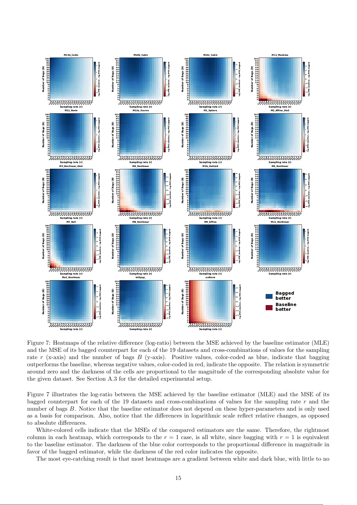
On the Use of Bagging for Lo cal In trinsic Dimensionalit y Estimation Krist´ of P ´ eter 1 Univ ersity of Southern Denmark Odense, Denmark krp@imada.sdu.dk OR CID: 0009-0008-1552-3361 Ricardo J. G. B. Camp ello 1 Univ ersity of Southern Denmark Odense, Denmark campello@imada.sdu.dk OR CID: 0000-0003-0266-3492 James Bailey 1 Monash Univ ersity Melb ourne, Australia james.a.bailey@monash.edu OR CID: 0000-0002-3769-3811 Mic hael E. Houle 1 New Jersey Institute of T ec hnology New ark, New Jersey , United States michael.houle@njit.edu OR CID: 0000-0001-8486-8015 Abstract The theory of Local Intrinsic Dimensionalit y (LID) has b ecome a v aluable tool for characterizing local com- plexit y within and across data manifolds, supporting a range of data mining and mac hine learning tasks. Accurate LID estimation requires samples dra wn from small neigh borho o ds around eac h query to a void biases from nonlocal effects and p oten tial manifold mixing, yet limited data within such neighborho ods tends to cause high estimation v ariance. As a v ariance reduction strategy , we propose an ensemble approac h that uses subbagging to preserv e the lo cal distribution of nearest neigh b or (NN) distances. The main challenge is that the uniform reduction in total sample size within each subsample increases the proximit y threshold for finding a fixed num b er k of NNs around the query . As a result, in the specific context of LID estimation, the sampling rate has an additional, complex in terplay with the neigh borho o d size, where b oth combined determine the sample size as well as the lo calit y and resolution considered for estimation. W e analyze b oth theoretically and exp erimentally ho w the choice of the sampling rate and the k -NN size used for LID estimation, alongside the ensemble size, affects p erformance, enabling informed prior selection of these hyper-parameters depending on application-based preferences. Our results indicate that within broad and well-c haracterized regions of the hyper-parameters space, using a bagged estimator will most often significantly reduce v ariance as well as the mean squared error when compared to the corresp onding non-bagged baseline, with controllable impact on bias. W e additionally prop ose and ev aluate dif- feren t w ays of com bining bagging with neighborho od smoothing for substantial further impro vemen ts on LID estimation p erformance. Keyw ords: Local Intrinsic Dimensionalit y · Bagging · Smo othing 1 In tro duction Lo cal Intrinsic Dimensionalit y (LID) is part of a broader notion of In trinsic Dimension (ID), whic h has been conceptu- alized in different w ays aiming to characterize the true complexity of a data space b ey ond its full represen tation dimen- sion, under the assumption that one or more data submanifolds may exist within that space [23, 13, 25, 41, 36, 42, 28]. One can think of LID as the minimum num ber of v ariables or effe ctive dimensions required to explain the underlying distribution at a particular lo cation of the data space, or the smallest dimension surface on whic h a sample from that distribution would lo cally lie on. It has found a growing num b er of applications, including outlier detection [7], similarit y searc h [8, 16], IoT in trusion detection [22], adversarial example analysis [38, 3], self-sup ervised learning regularization [30], graph embedding design [43], data segmentation [1], and gran ular deformation analysis [49], just to mention a few. A wide range of LID estimators has b een prop osed, among which a ma jor class is based on the extreme v alue theoretic (EVT) limiting distribution of distances as a neigh borho o d radius around a query location shrinks to zero — e.g., MLE, MoM, PWM, TLE [4, 6]. Other w ell-known approaches include MADA [20], ESS [32], and originally global ID estimators, suc h as TWO-NN [19], which can b e generalized to lo cally estimate LID [9]. The ab o ve techniques emplo y k -NN search for sampling around the query location, ho w ever, there are mo del-based alternatives — suc h 1 as LIDL (using approximate likelihoo d) [44] and FLIPD (employing diffusion mo dels) [34] — with different wa ys of quan tifying lo calit y . Despite their differences, most estimators ev aluate LID at a query location using only nearby observ ations to capture lo cal properties of the data space. Using fara wa y data p oin ts risks introducing nonlo cal biases, e.g., by mixing nearby manifolds with different dimensionalities, or violating lo cal isotrop y on an anisotropic surface — see Figure 1. In practice, given a finite size dataset, shrinking an arbitrary neighborho o d radius can lea ve to o few p oin ts inside, which tend to yield high-v ariance, unstable estimates; enlarging it reduces v ariance, but also pulls in nonlo cal structure that can increase bias. This bias-v ariance tradeoff is the central practical obstacle in LID estimation, and it can undermine downstream applications that critically rely on accurate, stable estimations of LID. T ackling this c hallenge through b ootstrapping-based statistical machinery , rather than simply trading v ariance with bias, is the main goal of this pap er. Figure 1: The leftmost figure shows the L ol lip op dataset [44] o verlaid w ith the cum ulative distribution function (c.d.f ) of the induced empirical distance distribution from the query at (2 , 2), as a heatmap. The 2nd figure shows that, within close vicinity to the query , t , the c.d.f. is prop ortional to the square of the distance, b ecoming linear b eyond the b ounds of the 2D (circle-plate) submanifold, when the 1D (line) submanifold is reac hed. The 3rd figure shows a heatmap of LID estimates at the query at (0 . 5 , 0 . 005) using MLE [5], as a function of the k -NN hyper-parameter, o verlaid with the corresp onding dataset distributed uniformly on a thin ribb on-like surface. The rightmost figure displa ys how LID estimates v ary with k , not only affected by the interpla y b etw een lo cality preserv ation and sample size, but also changing with the resolution at which it is measured in practice. Within close vicinity from the query , where neither lo calit y or resolution is critical, the small sample size results in high v ariance and — for estimators that are only asymptotically unbiased (including MLE) — also in bias. W e prop ose to adapt b o otstr ap aggr e gating (a.k.a. b agging for short) [17] as a metho d-agnostic, v ariance-reduction wrapp er for LID estimators. While bagging is a commonly used technique, e.g., in the context of decision trees [2] and ensembles more broadly , b oth shallow [50] and deep [21, 48], to the b est of our knowledge it has not b een applied to LID estimation b efore. In this sp ecific setting, the standard b eha vior of bagging is not trivially guaranteed. T o align with con tinuit y assumptions on the underlying data densit y and to preserv e the original distribution of distances, subsampling without replacement is required within each b ag (i.e., ensemble member), th us causing the in-bag sample size to be reduced. Reducing the sample size increases the distance threshold required to retrieve a fixed num b er k of neigh b oring p oints around a query , making it so that a fixed k on a subsample corresp onds to a larger effective NN radius, with p otential to introduce undesirable nonlo cal effects as v ariance decreases (e.g., see Figure 1). The problem has a close analogue in traditional EVT, where the chosen sample size determines the upp er-tail threshold. When estimating the extreme v alue index using the k largest order statistics, the choice of k trades v ariance (small k ) against bias (large k ), and subsample-b ootstrap methods sho w how the MSE-optimal k b et w een subsampled and full-sample estimators can be explicitly rescaled according to the sampling rate [39, 18]. This pro vides critical motiv ation in the current study for its exploration within the locality restrictions corresp onding to a low er-tail threshold for LID estimation. W e pro vide theoretical and empirical analyses of bagged LID estimation, fo cusing on how the n um b er of bags B and the sampling rate r , together with the lo calit y threshold (the neighborho od size k in case of NN-based LID estimators) jointly shap e bias, v ariance, and mean-squared error (MSE). W e show how the selection of these hyper- parameters can result in dramatic reduction of MSE, typically resulting from significan t reduction in v ariance with limited or no asso ciated compromise in bias. Our results supp ort that this is mainly enabled by the additional degree of freedom provided b y the sampling rate con trolling the tradeoff b et ween the bag size and the level of indep endence b et w een bags, which often allows for wider ranges of effective lo cality thresholds for LID estimation, and within whic h the bagged estimator can achiev e sup erior p erformance than the baseline equipp ed with its own MSE-optimal lo calit y threshold. This provides applic ation-sp e cific insigh ts as to wh y and how bagging can b e effectively used to mitigate the bias-v ariance dilemma in LID estimation. 2 Additionally , we ev aluate neighborho o d smoothing [15] as another strong standalone v ariance-reduction approach and show that it is complementary to bagging: applying smo othing within each bag (pre-smo othing) and/or after aggregation (p ost-smo othing) yields the most substantial MSE reduction in our exp eriments. Our con tributions can b e summarized as follo ws: • Introducing bagging for LID estimation. • Theoretical analyses shedding further light onto the effects and interactions of the h yp er-parameters gov erning the b eha vior of bagging. • Exp erimen tal analyses of the relationship b et ween bagging hyper-parameters as well as their p oten tial in terplay with the lo calit y threshold of LID estimators (demonstrated through the k h yp er-parameter of NN-based metho ds). • Exp erimen tal results on b enchmark datasets sho wing that bagging, as well as its combinations with smoothing, not only reduce v ariance but generally reduce the MSE of LID estimates compared to the baseline, in case of m utually optimal indep enden t selection of h yp er-parameters. 2 Related w ork V ariance reduction in LID estimation is addressed either by designing lo wer-v ariance estimators or by applying estimator-agnostic wrapp ers to stabilize existing metho ds. Next, w e review approac hes within these tw o categories. TLE [6] is closely related to EVT-based LID estimators such as MLE [5], but it mo difies the classic asymptotic distance-based lik eliho o d function by incorp orating non-central distance information to derive an extended statistic. It was shown to substantially reduce v ariance while maintaining comparable bias to MLE. How ever, TLE is tied to the EVT formulation and is not readily transferable as a generic wrapp er to arbitrary LID estimators. More general stabilization can be ac hiev ed via data pre-processing or by p ost-processing estimates. In [35], it has b een shown that pre-pro cessing by scale space filtering metho ds can contribute to LID estimation in the context of hypersp ectral imaging data. These techniques w ork by denoising the original dataset, thus reducing v ariance and, accordingly , resulting in more accurate and stable LID estimates. How ev er, the metho d is designed under assumptions sp ecifically related to the type of datasets in the in tended application of hypersp ectral images. A widely applicable p ost-processing approac h is neighborho od smo othing [47], which is easily translatable to LID estimation. Given p er-query LID estimates, regular smo othing replaces each by an a verage o ver their local neigh b orho od (e.g., k -NN), whic h can reduce v ariance assuming that neighboring p oin ts share similar LID. T o impro ve alignment with this assumption, the manifold adaptive neighborho od smo othing technique presented in [15] constructs the k -NN graph of the data p oin ts based on Euclidean distance; smo othing is then p erformed on a neigh b orho od of p oin ts based on their appro ximated geo desic distance to the query as the shortest paths along the graph, which lo cally approximates the query’s submanifold. Such ge o desic smo othing tec hnique has b een shown to reduce the v ariabilit y of the non-linear least-squares estimator describ ed in [15]. 3 Bac kground 3.1 LID LID can b e defined from a purely distributional p ersp ectiv e, b eyond the realm of any particular data sample, as a lo cal notion of ID at a given query lo cation. A theoretical, EVT-based approach to this concept that has gained increasing attention in recen t years has b een form ulated in [27, 29]. In this theoretical framework, for a selected query lo cation and distance metric, there exists a distribution of distanc es from the query that is induc e d from an underlying distribution of interest defined in the original data space. Under certain assumptions of lo calit y and smo othness, the limiting low er tail of the cumulativ e distribution function ( c.d.f. ) of such a theoretical distance distribution is fully and uniquely c haracterized by LID as a quantifiable prop ert y at the query . In this pap er, unless stated otherwise, this is the notion of LID that will b e implicitly assumed, e.g., in our exp erimen ts in volving practical LID estimation. Notice, ho wev er, that the bagging tec hniques in tro duced in this pap er are by no means estimator-sp ecific, but rather broadly applicable to virtually any LID estimator regardless of their supp orting LID paradigm. 3.2 Bagging Bagging is a resampling technique introduced b y Breiman [10] as a wa y of harnessing computational pow er to improv e the stability of mo dels and estimators by aggregating results across multiple resampled versions ( b ags ) of the original 3 data. It is esp ecially effectiv e for mo dels that are accurate on av erage but highly v ariable. Classic examples include bagging for decision trees and random forests [31, 11, 2], as well as a v ariety of mo dern deep learning applications [48, 21]. General theoretical results for the v ariance-reduction effect of bagging, including the subsampling v ariant adopted in the presen t pap er, can b e found in [12]. The term b agging is commonly referring to resampling with r eplac ement , where each bag can ha ve the same size as the original dataset and may contain duplicate samples. In our setting, ho wev er, duplicates w ould distort the distance distribution and violate its absolutely contin uous assumption underlying most LID estimators. W e therefore use the subb agging ( subsample aggr e gating ) v ariant, where sampling within an individual bag happens strictly without replacemen t and eac h bag th us contains a strictly smaller sample size than the whole dataset. F or this reason and for the sak e of simplicit y , in the remainder of this paper and unless explicitly stated otherwise, when referring to b agging we will assume the follo wing formal definition of subb agging , which coincides with that from [12]: Definition 1 (Subbagging) . Given n i.i.d. r andom ve ctors D ≜ ( X 1 , . . . , X n ) fol lowing a distribution over the ambi- ent sp ac e that r elates to a p ar ameter θ , let the n sample estimator of θ b e define d as a statistic ˆ θ n ≜ ˆ θ ( X 1 , . . . , X n ) . L et m = rn < n b e an inte ger for some sampling r ate r ∈ (0 , 1) and cr e ate B r andom subsets (a.k.a. bags ) of size m e ach, D i,m ≜ ( X Π ( i ) 1 , . . . , X Π ( i ) m ) for i = 1 , . . . , B , by subsampling fr om D using r andom index sets, Π ( i ) ≜ { Π ( i ) 1 , . . . , Π ( i ) m } . Such index sets Π ( · ) ar e i.i.d. (uniformly) over al l  n m  p ossible choic es of m differ ent indic es out of n . The b agge d estimator is then define d as: ˆ θ B ,m ≜ 1 B B X i =1 ˆ θ m,i ; wher e ˆ θ m,i ≜ ˆ θ ( X Π ( i ) 1 , . . . , X Π ( i ) m ) (3.1) 4 Bagged LID estimators T o translate Definition 1 to the sp ecific context of LID estimation, we consider the sample set D to corresp ond to our full dataset of n observ ed p oin ts in the R dim am bient space, whereas the baseline LID estimator at a fixed query p oin t q ∈ R dim , [ LI D ( q ), is considered to satisfy measurability assumptions and corresp onds to the statistic ˆ θ , such that [ LI D n ( q ) ≜ [ LI D n ( X 1 , . . . , X n ; q ) ≡ ˆ θ n ( X 1 , . . . , X n ) is the n -sample estimator at q . W e can thereby construct the bags D 1 ,m , . . . , D B ,m ⊂ D and the bagged estimator [ LI D B ,m ( q ) according to Definition 1. Figure 2 illustrates bagged LID estimation for a single query . Notice that most LID estimators are quantifiable at an y lo cation of the data space, albeit they are most often used only at query lo cations that coincide with p oin ts of the sample set ( q ∈ D ). After subsampling, a query p oin t q ∈ D will likely only b e present in some bags, but the bagged estimator will still require its individual estimation within each and every bag, regardless of whether the query is present or not. F rom an implementation viewpoint, the tw o different cases ha ve to be taken into consideration when a distance of zero b et ween the query location and a sample p oin t is not allow ed, such as for an y LID estimator under an absolutely con tinuous distance distribution assumption. F or the family of estimators based on the query’s k -NN, one needs to ensure that the nearest neighbor of a p oin t is nev er the p oint itself. In practice, this means that, whenever the query p oin t q is contained in the bag, it is not counted as its own neighbor (for estimating its LID within that bag) and, as such, it do es not count tow ards k , thus ensuring the same num b er of p oints k is alwa ys used for estimation. 4.1 Mean squared error (MSE) decomp osition The Mean-squared error (MSE) decomp osition is a well-kno wn result [45] that relates the theoretic MSE of an estimator to its bias and v ariance. It can b e used to gain deep er insights in to an estimator’s error b y looking at the tw o comp onen ts individually , as E[( ˆ θ B ,m − θ ) 2 ] = V ar( ˆ θ B ,m ) + (E[ ˆ θ B ,m ] − θ ) 2 . Notice that the ov erall bagged estimator will ha ve at most as large MSE as the m -sample estimator deplo yed within each bag, i.e., E[( ˆ θ B ,m − θ ) 2 ] ≤ E[( ˆ θ m,i − θ ) 2 ], whic h directly follo ws by recognizing that V ar( ˆ θ B ,m ) ≤ V ar( ˆ θ m,i ) and E[ ˆ θ B ,m ] = E[ ˆ θ m,i ] (see App endix A.2 for details). Ho wev er, in principle, this result alone do es not provide any improv ement guarantees for the bagged estimator with resp ect to the MSE of the n -sample estimator, which infers ov er the entire sample set D . When it comes to v ariance, [40] shows in the context of subbagging for decision trees that as the num b er of bags ( B ) tends to infinity , the v ariance of the bagged estimator decreases tow ards a known limiting v alue, which can b e expressed as the v ariance of the exp ectation of a single-bag estimator conditioned on the data, V ar(E( ˆ θ m,i | D )). In App endix A.2, we show more broadly (for any estimator following Definition 1) that this low er-limiting v ariance can also b e rewritten as the unconditional cov ariance b etw een single-bag estimators, Cov( ˆ θ m,i , ˆ θ m,j ). In Theorem 1, we formally outline how decreasing the sampling rate ( r ) is exp ected to cap the aforemen tioned limiting v ariance of the bagged estimator. The result is a combination of the well-kno wn Jensen-gap b ound [37] and 4 Figure 2: Flow c hart illustrating bagged LID estimation on a h yp othetical, toy dataset. The algorithm is display ed for a single query p oin t (with index 7) from the dataset. Note that it suffices to sample the bags only once and reuse them for differen t queries. The figure makes it clear that LID estimation can b e done indep endently for each query p oin t and for each bag, so pro cessing is highly parallelizable across multiple no des. F or details on estimation across a dataset of queries, see the pseudo co de in App endix A.1. the fact that the exten t of the ov erlap | Π ( i ) ∩ Π ( j ) | b et ween random index sets drawn without replacement follows the Hyp ergeometric Distribution [33, 24]. Theorem 1. Define γ ( h, m ) ≜ Co v( ˆ θ m,i , ˆ θ m,j | | Π ( i ) ∩ Π ( j ) | = h ) for the inte ger domain given by m = rn ∈ Z + and h = 0 , 1 , . . . , m , namely, the c ovarianc e of two single-b ag estimators given that we know the numb er of dep endent variables (pr ovide d that such a c ovarianc e exists and is finite for any p air of b ags). Assume that ther e exists a twic e differ entiable, incr e asing function φ : [0 , 1] → R such that ∀ h,m : h ≤ m γ ( h, m ) ≤ φ ( h m ) , then we have: ∀ r ∈ [0 , 1] Co v ( ˆ θ m,i , ˆ θ m,j ) ≤ φ ( r ) + O  1 n  (4.1) Pr o of. See pro of in App endix B.2 In simple terms, assuming that the magnitude of the conditional cov ariances γ ( h, m ) are roughly p ositiv ely prop ortional to the fraction of dep enden t v ariables b et ween the bags ( h/m ), Theorem 1 shows that we can set an implicit upper b ound on the limiting v ariance of the bagged estimator, lim B →∞ V ar( ˆ θ B ,m ) = Co v( ˆ θ m,i , ˆ θ m,j ), by reducing r and, accordingly , φ ( r ). This result suggests that w e can limit v ariance from abov e b y decreasing the sampling rate ( r ) and increasing the num b er of bags ( B ). How ever, recall that the resulting decrease in the bag size m can lead to more biased in-bag estimates, most noticeably , due to either fewer samples for LID estimation within a fixed lo cal vicinity around the query or, alternatively , a less lo cal vicinity con taining a fixed sample size k (e.g., see Figure 1). Since the exact nature of this bias-v ariance tradeoff is dep enden t on the particular LID estimator and its hyper-parameters (e.g., k ), as well as on the dataset in hand, exp erimen tal analyses are required to conclusively sho w the effects of bagging and its hyper-parameters in LID estimation. 5 Exp erimen tal metho dology 5.1 Estimators Alongside the classic MLE estimator as a standard baseline [4], w e also include TLE [6] and MAD A [20] to test the general applicability of bagging to different estimators without any inten t of promoting a particular metho d. TLE, while substan tially more computationally demanding, is designed to reduce v ariance, allowing us to test whether bagging can further enhance more sophisticated baselines already equipp ed with internal v ariance-reduction mech- anisms. T able 1 summarizes the tested estimators and their essential hyper-parameters, alongside the tw o wrapp er alternativ es to mitigate v ariance that w e exp erimen tally inv estigate in this pap er, namely , bagging and smo othing [15]. The goal is to compare each baseline against their own wrapp ed counterparts. 5 T able 1: LID estimators and hyper-parameters. “pre” and “p ost” sp ecify whether smo othing is applied to the in-bag LID estimates (i.e. prior to aggregation) or to the bagged LID estimates, resp. All other h yp er-parameters ha ve been previously defined. Baseline Baseline hyper-par. Bagging hyper-par. Smo othing strategy MLE [4] k r , B pr e or p ost TLE [6] k r , B pr e or p ost MAD A [20] k r , B pr e or p ost 5.2 Datasets As common practice in the LID literature, we use test datasets based on a foundational study of LID estimation on manifolds [26] later extended to a comprehensive benchmark framew ork in [14]. The data manifolds con tain n = 2500 p oin ts with known LID, whic h we use as ground truth when computing the MSE of estimators for ev aluation purp oses. W e additionally include the L ol lip op data from [44], and a high-dimensional Uniform dataset. More detailed descriptions of each dataset and a summary table are provided in App endix D. 5.3 Ev aluation measures W e measure the p erformance of LID estimators using the empirical MSE as well as its bias-squared plus v ariance decomp osition, for the reasons discussed in Section 4.1. Notice that in the presence of multiple ground-truth LID v alues across a dataset with different submanifolds, the MSE decomp osition needs to b e applied manifold-wise (details are provided in App endix C). 5.4 Bagging and smo othing exp erimen ts The first experiment ev aluates the o verall effectiv eness of bagging as w ell as compares and com bines it with smo othing , as an alternativ e or supplementary v ariance-reduction technique. W e obtain smoothed LID estimates for a query b y taking the arithmetic a verage of the estimates ov er its k -NN (the same neigh b orho od size used by the baseline estimator). This neighborho o d includes the query itself only when it is present in the reference sample set (bag or full dataset). When smoothing is p erformed on the baseline estimates, without any bagging, we will refer to it simply as smo othing . Additionally , we com bine bagging and smo othing in three different wa ys. The simplest idea is to smo oth out the aggregated bagged estimates themselv es, exactly as explained ab o ve, only no w for the bagged estimator. W e will refer to this com bination as “ p ost-smo othing ”. As an alternative approac h, we can instead smo oth out estimates based on each bag separately , determining the query’s k -NN among only the in-bag p oin ts. This wa y , smo othing takes place inside the bags, b efore the single-bag estimates are aggregated. W e refer to this combination as “ pr e-smo othing ”. Finally , we can also integrate both strategies ab o ve by simultaneously applying pre-smo othing ( pr e ) and p ost-smoothing ( p ost ). This go es to show that bagging and smo othing are not necessarily comp etitors. Bagging actually offers new a ven ues for applying smo othing in differen t wa ys. W e apply bagging, smo othing, and their three combinations indep enden tly to the different baseline estimators in T able 1, with the go al to c omp ar e e ach b aseline to their b agge d/smo othe d c ounterp arts, r ather than against e ach other . F or each case, we sweep the lo calit y hyper-parameter ov er a 9-step geometric progression from k = 5 to k = 72. F or bagged v arian ts, we additionally sweep the sampling rate o ver a 9-step geometric progression from r = 0 . 042 to r = 0 . 6, ev aluating all combinations of ( k , r ). W e are fixing the num b er of bags to B = 10, noting that increasing B can only further improv e results in fa vor of bagging. Then, for each dataset and metho d v ariant, we individually select the hyper-parameter setting that minimizes MSE: k for baseline/smo othing, and ( k , r ) for all bagged v ariants, comparing the metho ds at their b est observed p erformance. 5.5 Bagging h yp er-parameters exp eriments The second set of exp eriments fo cuses sp ecifically on bagging and explores how the choice of its hyper-parameters affects performance in terms of MSE, v ariance, and bias. These effects are discussed using the bagged MLE estimator. The results for MAD A and TLE (in App endix E) exhibit similar trends and the main conclusions do not c hange: 1st test (sampling rate): W e saw in Theorem 1 how decreasing r is exp ected to de-correlate the bags, and under certain general assumptions, reduce v ariance. Confirming this exp ected decrease in v ariance in the LID s etting and to what exten t it can ov ershine any p oten tial increase in bias as a function of the sampling rate ( r ) are the main goals of this exp erimen t. 6 Figure 3: Comparison of the relativ e MSE achiev ed b y three different LID estimators, MLE, TLE, and MAD A, with and without smo othing, bagging, and three strategies for combining bagging with smo othing. The results are for 19 datasets using case-by-case optimal k and r hyper-parameters. The min-max normalized MSE v alues are subtracted from 1 b efore plotting, suc h that larger scores corresp ond to smaller relative MSEs. F or this test, we chose a fixed k = 10 for the baseline estimators, a relatively small v alue compared to the dataset size, to attain to the general imp ortance of lo cality surrounding LID estimation. The effects of r ma y b e exaggerated or reduced depending on k ; how ever, it is worth stressing that the general trends remain the same and the main conclusions with resp ect to r do not change for different, fixed v alues of k . 2nd test (in teraction betw een k and r ): As previously discussed, b oth k and r affect the radius determining the lo cal neighborho od around the query used for estimation, which is directly prop ortional to k and inv ersely prop ortional to r , with the p otential to affect bias through non-lo cal effects and sample size. On the other hand, v ariance is generally in versely prop ortional to k and directly proportional to r . If both hyper-parameters are v ariable, then the v alues of k that result in more fav orable bias-v ariance tradeoffs will dep end on r and vice versa. Since the exact relationship may b e complex and p ossibly b oth dataset- and estimator-dep enden t, the goal of this exp erimen t is to identify ma jor general trends allowing clear guidance on the combined choice of these h yp er-parameters. W e ev aluate the bagged estimator ov er a grid of ( k , r ) combinations, comparing each against the baseline with the same k . The resulting MSE differences reveal ranges of r (and ratios k /r ) for which bagging improv es or worsens p erformance. Additional tests (n umber of bags): Analogous exp erimen tal setups and analyses demonstrating the (more straigh tforward) effects of the n um b er of bags ( B ) and its interaction with r are av ailable in App endices A.3 and A.4. 5.6 Co de and data a v ailabilit y A full co de that can b e used to repro duce all results in our pap er is av ailable from our GitHub page at h ttps://github.com/Campello-Lab/Bagging for LID, which also con tains all the datasets used in our exp erimen ts. Most of these datasets were generated using the Scikit-dimension [9] public Python library , which was also the source co de for the baseline LID estimators adopted in this study . 6 Results and discussion 6.1 Bagging and smo othing results Figure 3 shows the results for the first exp erimental setup in Section 5.4. W e use radar charts to display the optimal MSE v alues, min-max normalized across v arian ts, separately for each dataset, in rev erse. 1 Th us, scores lie in [0 , 1], where 1 denotes the lo west relativ e MSE and 0 the highest, therefore, larger co v ered area indicates b etter performance. There is a v ery clear trend. First, b oth bagging and smo othing impro v e o ver the baseline in almost all cases when used indep enden tly , with only one exception (TLE on M7 Roll), noting that smo othing is often the stronger standalone v ariant in these exp erimen tal conditions. Second, it is clear that combining them yields further gains, with a common p erformance ordering, consistently across the baselines: baseline < bagged < smo othed < bagged with p ost-smoothing < bagged with pre-smo othing < bagged with pre- and p ost-smo othing. Therefore, the main conclusion is that not only do b oth bagging and smo othing achiev e their purp ose on their o wn, but com bining them pro vides further impro vemen ts. 1 T ables of the raw MSE v alues are rep orted in App endix E.1. 7 3 6 9 12 15 18 M10a_Cubic 0 8 16 24 32 40 M10b_Cubic 0 15 30 45 60 75 M10c_Cubic 0.00 0.25 0.50 0.75 1.00 1.25 M11_Moebius 0 10 20 30 40 50 M12_Norm 0.0 0.2 0.4 0.6 0.8 1.0 M13a_Scurve 0 3 6 9 12 15 18 M1_Sphere 0.0 0.4 0.8 1.2 1.6 2.0 M2_Affine_3to5 0.0 0.8 1.6 2.4 3.2 4.0 M3_Nonlinear_4to6 0.0 0.8 1.6 2.4 3.2 4.0 4.8 M4_Nonlinear 0.0 0.6 1.2 1.8 2.4 3.0 3.6 M5b_Helix2d 0.0 2.5 5.0 7.5 10.0 12.5 15.0 M6_Nonlinear 0.05 0.09 0.18 0.33 0.62 1.00 0.0 0.2 0.4 0.6 0.8 1.0 M7_Roll 0.05 0.09 0.18 0.33 0.62 1.00 0 10 20 30 40 50 60 M8_Nonlinear 0.05 0.09 0.18 0.33 0.62 1.00 0 8 16 24 32 40 48 M9_Affine 0.05 0.09 0.18 0.33 0.62 1.00 0 8 16 24 32 40 Mn1_Nonlinear 0.05 0.09 0.18 0.33 0.62 1.00 0 15 30 45 60 75 Mn2_Nonlinear 0.05 0.09 0.18 0.33 0.62 1.00 0.00 0.15 0.30 0.45 0.60 0.75 0.90 lollipop_ 0.05 0.09 0.18 0.33 0.62 1.00 0 30 60 90 120 150 180 uniform V ariance Bias² Sampling rate (r) MSE Figure 4: MSE and its decomp osition for each of the 19 datasets as a function of the sampling rate r used for bagged MLE as the LID estimator. Note that the baseline MLE is equiv alent to r = 1, display ed on the righ tmost bar of the individual charts. 6.2 Sampling rate results (1st test on hyper-parameters): Figure 4 illustrates the exp erimen tal b eha vior of the MSE decomp osition for bagging as a function of the sampling rate r . The exact relationship is dataset-dep endent, but in general, by decreasing r (right-to-left along the x-axis) w e observe that: (i) bias 2 (green sub-bars) tends to increase or stay relatively stable in most cases; and (ii) v ariance (red sub-bars) shows a highly consistent, decreasing b eha vior. This robust effect on v ariance reduction supp orts the v alidity of our assumptions in Theorem 1 and confirms the bag de-correlating b enefits of reducing r . The opp osing trends often yield an intermediate “sweet sp ot” where an optimal bias-v ariance tradeoff is achiev ed in terms of a minimal MSE, confirming our arguments in Section 4.1. How ever, for some datasets (M10a Cubic, M13 Scurve, M1 Sphere, M2 Affine 3to5, M3 Nonlinear 4to6, and M8 Nonlinear), smaller r reduced b oth v ariance and bias, so the b est MSE o ccurred at the smallest tested r , suggesting that p oten tial non-lo cal biases asso ciated with decreasing r did not manifest within the given range of r v alues in those datasets. Ov erall, the exp erimen t mostly confirms the anticipated b eha vior for r , noting that results that were somewhat surprising, actually did so in a fa vorable wa y . 6.3 In teraction b etw een k and r results (2nd test on hyper-parameters): Figure 5 illustrates how the bagged LID estimator’s p erformance dep ends jointly on the baseline’s k -NN hyper- parameter and the sampling rate. As previously conjectured, the bias increase from the expansion of the effective lo cal neighborho o d radius, for sufficien tly large k comp ounding with sufficiently small r , may ov erp o w er the com bined v ariance reduction caused by b oth these settings, p otentially resulting in a larger MSE for the bagged estimator than the baseline. Ov erall, the heatmaps in Figure 5 confirm this exp ectation, as for most datasets, the hyper-parameter space is divided along a certain left-to-right upw ards white line where the tw o estimators achiev e similar MSEs. T o the righ t of this line, bagging tends to win out, while to the left, the baseline tends to perform better. This suggests that there is some dataset sp ecific constant, for which, if the ratio b et ween the tw o h yp er-parameters ( k r ) sta ys under, then w e can exp ect the bagged estimator to pro duce fav orable results, while the results are most likely not desirable otherwise. W e additionally observ e that the strongest gains usually o ccur at the b ottom-left region (small k , small r ), where bagging can strongly reduce MSE by sim ultaneously de-correlating bag estimates while preserving reasonable lo calit y . The experiment also clarifies ho w in the previous test with a v ariable r , fixing k = 10 may hav e caused partially unexp ected results for some datasets, as non-lo cal effects were not yet expressed. 6.4 Main tak eaw ays F rom our theoretical and experimental findings, w e pro vide the following guidelines for selecting the h yp er-parameters of bagging ( B , r ) with resp ect to the degree of lo calit y for LID estimation (quantified by the k hyper-parameter of the family of NN-based estimators adopted in this study): • Number of bags ( B ) : It is well-kno wn that increasing B has a strictly b eneficial but diminishing effect in terms of estimator v ariance (see Section 4.1), and this has b een confirmed in our exp erimen ts (App endices A.3 8 5 9 18 33 62 100 M10a_Cubic M10b_Cubic M10c_Cubic M11_Moebius M12_Norm M13a_Scurve M1_Sphere 5 9 18 33 62 100 M2_Affine_3to5 M3_Nonlinear_4to6 M4_Nonlinear M5b_Helix2d M6_Nonlinear M7_Roll 0.05 0.09 0.18 0.33 0.62 1.00 M8_Nonlinear 0.05 0.09 0.18 0.33 0.62 1.00 5 9 18 33 62 100 M9_Affine 0.05 0.09 0.18 0.33 0.62 1.00 Mn1_Nonlinear 0.05 0.09 0.18 0.33 0.62 1.00 Mn2_Nonlinear 0.05 0.09 0.18 0.33 0.62 1.00 lollipop_ 0.05 0.09 0.18 0.33 0.62 1.00 uniform 0.05 0.09 0.18 0.33 0.62 1.00 A verage Bagged better Baseline better 3 2 1 0 1 2 3 3 2 1 0 1 2 3 3 2 1 0 1 2 3 2 1 0 1 2 4 2 0 2 4 2 1 0 1 2 3 2 1 0 1 2 3 3 2 1 0 1 2 3 2 1 0 1 2 1.0 0.5 0.0 0.5 1.0 3 2 1 0 1 2 3 2 1 0 1 2 2 1 0 1 2 3 2 1 0 1 2 3 3 2 1 0 1 2 3 3 2 1 0 1 2 3 3 2 1 0 1 2 3 2 1 0 1 2 3 2 1 0 1 2 3 2 1 0 1 2 Sampling rate (r) k log (MSE_baseline) log (MSE_bagged) Figure 5: Heatmaps of the relative difference (log-ratio) b et w een the MSE ac hieved by the baseline estimator (MLE) and the MSE of its bagged counterpart for e ac h of the 19 datasets and cross-combinations of v alues for the sampling rate r (x-axis) and the k -NN neighborho o d size k (y-axis). P ositive v alues, color-co ded as blue, indicate that bagging outp erforms the baseline, whereas negativ e v alues, color-coded in red, indicate the opp osite. The relation is symmetric around zero and the darkness of the cells are prop ortional to the magnitude of the corresp onding absolute v alue for the given dataset. and A.4). Since the resulting gains come with no counter-effect in terms of bias, this hyper-parameter is not critical. How ever, the runtime complexity of the bagged estimator is linearly dep enden t on B (see Section 7). Our exp erimen ts consistently supp ort that increasing B b eyond 10 is only recommended if one strongly fav ors further diminishing gains in stability ov er runtime. • Sampling rate ( r ) and lo cality ( k ) : As anticipated in Section 4.1 and confirmed by our exp erimen ts, the h yp er-parameters k and r jointly control the bias-v ariance tradeoff. If the primary goal is to bind v ariance reduction in the bagged estimator to a p ositiv e (or at least neutral) o verall impact in terms of MSE as compared to the baseline, our results supp ort combining lo w v alues of both k and r . In practice, we suggest to set k roughly within [5 , 10] or so as a minimal lo cal sample size for LID estimation, then choose r accordingly , roughly within [ r min , 0 . 5]. The low end of this range should ensure that the in-bag subsamples are still representativ e enough of the relev ant structures in the dataset (e.g., manifolds, classes, clusters) and, as suc h, it is problem-dependent. Within the (MSE-orien tated) rough ranges of k and r suggested abov e, for a fixed chosen k decreasing r is theoretically exp ected to decrease v ariance (Theorem 1), often at the exp ense of bias. In the context of LID, applications that can tolerate large estimation biases, e.g., requiring mostly a reliable ordering for the purp ose of relative comparisons of LID v alues across different queries, may b enefit from smaller sampling rates (closer to r min ), whereas in applications where systematic LID offsets can b e critically detrimental, one might prefer larger, more conserv ativ e rates. 7 Complexit y analysis In this section, we summarize the time complexit y of bagging for LID estimation (in a non-parallel setting). An extended analysis, including the different smo othing v ariants (bagging with pre/p ost-smoothing) is deferred to Ap- p endix A.5. Let p ( n ) denote the runtime cost of computing a baseline LID estimate for a single query using a sample of size n . Therefore, the total runtime complexit y for the baseline estimator (no bagging), T base , is O ( n p ( n )) when taken o ver n different query lo cations. Bagging with B bags of size m = r n , for a single query , ev aluates the estimator on eac h bag and a verages, resulting in O ( B p ( r n )) time, where the sampling step for bag construction and final a veraging con tribute only low er-order terms ( O ( B nr ) and O ( B )) and can thu s b e omitted. As the bags do not hav e to b e resampled p er-query , the total runtime complexit y of the bagged estimator taken o ver n queries, T bag , is simply O ( B n p ( r n )). 9 F or the wide family of NN-based LID estimators, p ( n ) is dominated by finding the k -NN of the query in the sample set of size n , where k is assumed to b e either constant or k << n . Using a naive exhaustive search, p ( n ) is O ( n ), which translates to T base → O ( n 2 ) and T bag → O ( B r n 2 ). F or large enough n , bagging may b e faster as long as r < 1 /B . Assuming a more sophisticated (indexed) search strategy , with av erage estimation time p ( n ) of order O (log n ) p er query (amortized ov er all queries), then T base → O ( n log n ) and T bag → O ( B n log ( rn )). 8 Limitations and future work The ob jective ev aluation measures we used, namely , MSE, V ariance and Bias, re quired datasets commonly used for b enc hmarking, with ground-truth LID. While these datasets undoubtedly pose a challenge for estimators, due to their manifold curv atures within higher-dimensional space s, they may not fully span the sp ectrum of complex b eha viors found in real data. Therefore, LID bagging, smo othing, and their combinations as prop osed in this pap er, are y et to b e fully tested in practical scenarios with p oten tially more complex data distributions, noise, and related challenges. Without ground-truth LID though, this will require indirect ev aluation in downstream task applications, whic h is left for future w ork. In future work, w e also in tend to in vestigate the use of the out-of-bag (OOB) samples from eac h bag for ev aluation and (unsup ervised) mo del selection. 9 Conclusions W e proposed bagging as a v ariance reduction strategy for LID estimation, alongside different strategies for its com bination with neigh b orhoo d smo othing. W e theoretically and experimentally explored the b ehavior of bagged LID estimators, with esp ecial focus on the in terplay betw een the sampling rate r and the locality threshold (neigh b orhoo d size k ), whereby in-depth analyses of their joint effect on v ariance, bias, and ov erall MSE hav e b een provided. Our results sho w that within a wide range of these hyper-parameters, clearly characterized b y small v alues of k and small- to-mo derate v alues of r , the bagged estimator is not only exp ected to reduce v ariance but it also tends to outp erform the corresp onding baseline estimator in terms of MSE. The higher level of freedom made av ailable by these hyper- parameters in con trolling the bias-v ariance tradeoff also allows a reduction in MSE to b e systematically observ ed when comparing the indep endently optimal bagged and baseline estimators, i.e., when they are indep endently set to their b est preferred hyper-parameter v alues for eac h dataset. These impro vemen ts hav e been achiev ed across differen t baseline LID estimators and with a num b er of bags as small as 10, which comes with little to none additional computational price. Finally , our results robustly show that significan t further impro vemen ts in performance can b e achiev ed by combining bagging with neighborho od smo othing, which systematically outp erforms b oth standalone approac hes. 9.1 Use of Generative AI W e used ChatGPT 5.4 strictly to assist with language style and c onciseness. 9.2 Disclosure of Interests The authors hav e no comp eting interests to declare that are relev ant to the conten t of this article. 10 A Supplemen tary con tributions A.1 Bagging for LID Algorithm Belo w is the general algorithm for bagged LID estimation across the whole sample set D considered as query lo cations, as referenced by the main pap er in Section 4. Algorithm A.1 shows that one efficien t wa y of handling the problem of the query b eing in the bag or otherwise is to lo op ov er the p oin ts of the given bag, and then its corresp onding complement (also known as the out-of-b ag ). This w ay , w e av oid the need to c heck for inclusion/exclusion for each query-bag com bination. This is esp ecially helpful when the estimator is based on ordered nearest neighbor (NN) distances, in which case, definite knowledge of q ∈ D i,m or q / ∈ D i,m can help us decide if the smallest distance should b e considered for estimation or not, even if NN distance calculation is only appro ximate. Algorithm 1 Bagged LID estimator across all queries Input: D ∈ R n × dim , 1 << n ∈ Z + , dim ∈ Z + , r ∈  1 n , 1  , B ∈ Z + Require: Baseline LID estimator oracle [ LI D n : R n × dim × R dim → R 1: m ← ⌈ n · r ⌉ 2: for i = 1 to B do 3: Sample π ( i ) ∼ Π (uniformly ov er all  n m  p ossible c hoices of m different indices out of n ) 4: D i,m ←  D [ π ( i ) 1 ] , . . . , D [ π ( i ) m ]  5: end for 6: for i = 1 to B do 7: for q ∈ D i,m do 8: [ LI D m,i ( q ) ← [ LI D m − 1 ( D i,m \ { q } ; q ) 9: end for 10: for q ∈ D \ D i,m do 11: [ LI D m,i ( q ) ← [ LI D m ( D i,m ; q ) 12: end for 13: end for 14: for q ∈ D do 15: [ LI D B ,m ( q ) ← 1 B P B i =1 [ LI D m,i ( q ) 16: end for 17: return h [ LI D B ,m ( D [1]) , . . . , [ LI D B ,m ( D [ n ]) i A.2 Bagging theory revisited In the following, w e discuss tw o results that show the general effectiv eness of bagging and demonstrate the roles of its h yp er-parameters, namely , the num b er of bags, B , and the sampling rate, r ≜ m/n ∈ (0 , 1), as supp orting material to the theoretical analysis in Section 4 of the main pap er: • Theorem 2 fo cuses on the asymptotic v ariance reduction effect of increasing the num b er of bags, and has analogous or similar results av ailable in the literature, usually in the general context of classifiers or decision trees, for example, in [40], which also examines prop erties of the s ubbagging alternative. Ho wev er, the current form ulation in the sp ecific context of parameter estimation is particularly conv enient within our scop e to in terpret/explain our results. • Theorem 1 is concerned with the v ariance reduction prop erty of decreasing the sampling rate, and is already presen ted in the main pap er; how ev er, this section of the app endix offers additional insights and explanations to help with in terpreting its assumptions and its claims. Theorem 2. L et ˆ θ m,i and ˆ θ m,j b e the single b ag estimators for b ags i and j ( i  = j ) of a mutual sample set D , r esp e ctively, as define d in 1. Then, the fol lowing expr essions hold for the unc onditional varianc e of the b agge d estimator, V ar( ˆ θ B ,m ) , define d over ( D , Π (1) , . . . , Π ( B ) ) : Co v ( ˆ θ m,i , ˆ θ m,j ) ≤ V ar( ˆ θ B ,m ) = V ar( ˆ θ m )  ρ m + 1 − ρ m B  ≤ V ar( ˆ θ m ) and V ar( ˆ θ B ,m ) → Co v( ˆ θ m,i , ˆ θ m,j ) as B → ∞ (A.1) 11 where ρ m ≜ Corr( ˆ θ m,i , ˆ θ m,j ) and Co v ( ˆ θ m,i , ˆ θ m,j ) stand for the correlation and co v ariance of the single bag estimators, resp ectiv ely . Pr o of. See pro of in Section B.1. Theorem 2 illustrates the v ariance profile of the bagged estimator in terms of the num b er of bags ( B ) and sho ws that it is limited b etw een the cov ariance of the single bag estimators (as a low er-b ound) and the v ariance of the m sample estimator ˆ θ m (as an upp er-bound). Assuming that for some m ′ w e hav e Cov( ˆ θ m ′ ,i , ˆ θ m ′ ,j ) < V ar( ˆ θ n ), then b y prop erly selecting the sampling rate r suc h that m ′ = n · r and using a sufficiently large B , improv ement can b e ac hieved in relation to the n sample estimator as the bagged estimator v ariance tends to the smaller Cov( ˆ θ m ′ ,i , ˆ θ m ′ ,j ) limiting v alue. It is worth noticing that while using a smaller subsample size m (or equiv alently , a smaller sampling rate r ) tends to increase the upp er-b ound term, V ar( ˆ θ m ), it conv ersely tends to decrease the low er-b ound term, Cov( ˆ θ m,i , ˆ θ m,j ), b y increasing the level of indep endence b etw een the bags. Giv en that the v ariance of the bagged estimator conv erges to wards the latter as we increase the n umber of bags, this result suggests that low sampling rates asso ciated with a large num b er of bags would allow for v ariance reduction as compared to the n sample estimator. Of course, this result does not sa y anything in terms of bias. How ever, under the assumption that the n sample estimator is un biased (p oten tially asymptotically as n increases), then so is the m sample estimator and (trivially from (3.1)) the bagged estimator as well. Recalling Theorem 1 it is clear that, asymptotically as n → ∞ (i.e., as the size of the original sample set D tends to infinity), the theoretical lo wer limiting v alue for the v ariance of the bagged estimator as stated in Theorem 2, Co v ( ˆ θ m,i , ˆ θ m,j ), is b ounded from ab o ve by an increasing function of r , as long as the assumptions in the theorem hold. In simple terms, Theorem 1 says that if the estimator and data are such that the magnitude of the conditional bag cov ariances γ ( h, m ) are roughly p ositively prop ortional to the fraction of dep enden t v ariables b et ween the bags ( h/m ), then from Theorem 1 we can exp ect to b e able to reduce the upp er b ound on unconditional bag cov ariance (lo wer limiting v ariance of the bagged estimator) b y decreasing the sampling rate ( r ). The assumption is natural in the sense that it captures our intuition ab out the cov ariance of the dep enden t estimators: if a small (large) p ortion of v ariables are dep endent, we exp ect low er (higher) cov ariance. If all v ariables are indep endent, i.e. h m = 0, then the cov ariance is 0, while if they are all dep enden t, i.e. h m = 1, then the cov ariance is maximized as v ariance. F or v alues in b et ween, so when 0 < h m < 1, we can intuitiv ely exp ect a roughly increasing relationship in terms of h m , and this notion is captured by the assumed upp er-bound. By knowing more ab out the b ehavior of θ and therefore γ ( h, m ), we could p ossibly choose φ in such a wa y that it is a go o d approximation of γ ( h, m ), yielding a tight upper-b ound. Apart from particular choices and their usefulness (or lack thereof ) for sp ecific purp oses, for the sake of explaining the o verall relationship in terms of the sampling rate, this general theorem suffices. Note that b y the nature of the expression for V ar( ˆ θ B ,m ) in (A.1), increasing the num b er of bags ( B ) has diminishing returns, dep ending on the magnitude of ρ m . In case of relatively large ρ m , the 1 − ρ m B term accounts for a decreasingly lo wer p ortion of the v ariance, thence B has prop ortionally less impact, while the increase in runtime remains linear. Notably , according to (4.1), ρ m · V ar( ˆ θ m ) could b e exp ected to decrease when decreasing the sampling rate ( r ). Dep ending on the data and estimator, this gives reason to exp ect a larger improv emen t from increasing B , for low er v alues of r . F or each dataset and estimator, the exact b ehavior of the b ounds in (A.1) and (4.1) can b e different, therefore, exp erimen tal analyses are required to show the effectiveness of bagging in sp ecific application scenarios, such as LID estimation in this pap er. A.3 Additional exp erimen tal setups This section introduces tw o additional exp erimen tal setups dealing with the role of the num b er of bags hyper- parameter and its interaction with the sampling rate, to confirm the theoretical predictions of Theorem 2 and Theorem 1 in the context of bagged LID estimation. This serves to complete the bagging hyper-parameter selection exp erimen ts in Section 5 of the ma in pap er, which fo cused on the particular role of the sampling rate and its in teraction with the k nearest neighbor ( k -NN) lo calit y hyper-parameter of certain baseline estimators (e.g., MLE). As explained in the main pap er, these exp erimen ts are sp ecifically ab out bagging, designed to explore how exactly the choice of its h yp er-parameters affects p erformance in terms of MSE, v ariance, and bias, when applied in the context of LID estimation. W e show and discuss these effects on the bagged MLE estimator; how ever, the results for MADA and TLE exhibit similar general trends and can b e found in Section E. They hav e b een sidelined for the sak e of clarity and compactness, since the main conclusions do not c hange. The results of these exp eriments are presen ted and analyzed in Section 6 and serv e as the exp erimen tal basis for our prop osed hyper-parameter selection guidance with regards to the num b er of bags hyper-parameter as presented in the main pap er. 12 3rd test (num b er of bags): As shown in Theorem 2, increasing the num b er of bags ( B ) is most effective when estimates from different bags are low-correlated, which in turn tends to asso ciate with low er sampling rates, as seen in Theorem 1. Therefore, for the current exp erimen t, we fix the sampling rate at a relatively small v alue, r = 0 . 05, allo wing for B to range from 3 to 400 according to a 20 step geometric progression. 2 The progression enables us to see the effect of the hyper-parameter according to prop ortional increases, while exploring a wide range of v alues. W e mainly exp ect to observe the diminishing returns of increasing B as predicted by Theorem 2 and discussed in Section A.2. The results of this exp erimen t are presen ted and analyzed in Section A.4.1 4th test (interaction b et w een B and r ): These exp eriments are meant to test the interpla y b etw een the tw o h yp er-parameters B and r , combining observ ations from the 1st sampling-rate test, presented in the main pap er, and the previously discussed num b er of bags test, to sho w in practice the interacting effects we had already anticipated and discussed previously in Section A.2. They are also intended to test the robustness of bagging in terms of a sustained p erformance across wide ranges of hyper-parameter c hoices and com binations. W e calculate bagged estimators for every combination of hyper-parameter v alues, b etw een the 20 v alues of sam- pling rates used in the previous exp erimen ts in this section, and a more comprehensive progression for the num b er of bags, b et ween 1 and 100, b oth follo wing roughly the same geometric rate. The results of this exp erimen t are presen ted and analyzed in Section A.4.2. 2 W e also include the Baseline case as the first exp eriment. 13 A.4 Supplemen tary result analysis A.4.1 Num b er of bags (3rd test) Baseline 3 4 5 6 8 11 14 18 24 30 39 51 66 85 110 143 185 239 309 400 Number of Bags (B) 0 3 6 9 12 15 18 MSE M10a_Cubic Baseline 3 4 5 6 8 11 14 18 24 30 39 51 66 85 110 143 185 239 309 400 Number of Bags (B) 0 8 16 24 32 40 MSE M10b_Cubic Baseline 3 4 5 6 8 11 14 18 24 30 39 51 66 85 110 143 185 239 309 400 Number of Bags (B) 0 15 30 45 60 75 MSE M10c_Cubic Baseline 3 4 5 6 8 11 14 18 24 30 39 51 66 85 110 143 185 239 309 400 Number of Bags (B) 0.0 0.3 0.6 0.9 1.2 1.5 1.8 MSE M11_Moebius Baseline 3 4 5 6 8 11 14 18 24 30 39 51 66 85 110 143 185 239 309 400 Number of Bags (B) 0 10 20 30 40 50 MSE M12_Norm Baseline 3 4 5 6 8 11 14 18 24 30 39 51 66 85 110 143 185 239 309 400 Number of Bags (B) 0.0 0.2 0.4 0.6 0.8 1.0 MSE M13a_Scurve Baseline 3 4 5 6 8 11 14 18 24 30 39 51 66 85 110 143 185 239 309 400 Number of Bags (B) 0 3 6 9 12 15 18 MSE M1_Sphere Baseline 3 4 5 6 8 11 14 18 24 30 39 51 66 85 110 143 185 239 309 400 Number of Bags (B) 0.0 0.4 0.8 1.2 1.6 2.0 MSE M2_Affine_3to5 Baseline 3 4 5 6 8 11 14 18 24 30 39 51 66 85 110 143 185 239 309 400 Number of Bags (B) 0.0 0.8 1.6 2.4 3.2 4.0 MSE M3_Nonlinear_4to6 Baseline 3 4 5 6 8 11 14 18 24 30 39 51 66 85 110 143 185 239 309 400 Number of Bags (B) 0 1 2 3 4 5 6 MSE M4_Nonlinear Baseline 3 4 5 6 8 11 14 18 24 30 39 51 66 85 110 143 185 239 309 400 Number of Bags (B) 0.0 0.6 1.2 1.8 2.4 3.0 3.6 MSE M5b_Helix2d Baseline 3 4 5 6 8 11 14 18 24 30 39 51 66 85 110 143 185 239 309 400 Number of Bags (B) 0.0 2.5 5.0 7.5 10.0 12.5 15.0 MSE M6_Nonlinear Baseline 3 4 5 6 8 11 14 18 24 30 39 51 66 85 110 143 185 239 309 400 Number of Bags (B) 0.0 0.3 0.6 0.9 1.2 1.5 1.8 MSE M7_Roll Baseline 3 4 5 6 8 11 14 18 24 30 39 51 66 85 110 143 185 239 309 400 Number of Bags (B) 0 10 20 30 40 50 60 MSE M8_Nonlinear Baseline 3 4 5 6 8 11 14 18 24 30 39 51 66 85 110 143 185 239 309 400 Number of Bags (B) 0 8 16 24 32 40 48 MSE M9_Affine Baseline 3 4 5 6 8 11 14 18 24 30 39 51 66 85 110 143 185 239 309 400 Number of Bags (B) 0 8 16 24 32 40 MSE Mn1_Nonlinear Baseline 3 4 5 6 8 11 14 18 24 30 39 51 66 85 110 143 185 239 309 400 Number of Bags (B) 0 15 30 45 60 75 MSE Mn2_Nonlinear Baseline 3 4 5 6 8 11 14 18 24 30 39 51 66 85 110 143 185 239 309 400 Number of Bags (B) 0.00 0.15 0.30 0.45 0.60 0.75 0.90 MSE lollipop_ Baseline 3 4 5 6 8 11 14 18 24 30 39 51 66 85 110 143 185 239 309 400 Number of Bags (B) 0 40 80 120 160 200 MSE uniform V ariance Bias² Figure 6: MSE and its decomp osition for eac h of the 19 datasets, as a function of the num b er of bags B used for bagging of MLE as the baseline LID estimator (display ed on the leftmost bar of the individual charts). See Section A.3 for the detailed exp erimen tal setup. Figure 6 illustrates the exp erimental b ehavior of the MSE decomp osition for bagging as a function of the num b er of bags B . The exp erimen t confirms our exp ectation that increasing B : (i) do es not systematically affect bias; and (ii) it reduces v ariance according to the general trend supp orted by Theorem 2, that is, at a diminishing rate. Regarding the latter, notice that despite the geometric progression of B in the x-axis, the largest prop ortional drops in v ariance (red sub-bars) mostly happ en at the b eginning. While bias 2 (gree sub-bars) is not systematically affected by B , in most cases we observe a difference b et ween the bias for the baseline estimator (leftmost bar) and the rest (bagged estimators). This difference can b e in fav or of either the bagged or the baseline estimator, as in the current test we fix the k and r hyper-parameters, causing a dataset-dep enden t bias b eha vior. It is exp ected that certain hyper-parameter combinations will b e b etter for the baseline than the bagged estimator or vice-v ersa, which we further analyze in detail in Section 6 of the main pap er. 14 A.4.2 In teraction b et w een B and r (4th test): 0.05 0.06 0.07 0.08 0.09 0.11 0.13 0.15 0.18 0.21 0.24 0.28 0.33 0.39 0.45 0.53 0.62 0.73 0.85 1.00 Sampling rate (r) 1 2 3 4 5 6 7 8 10 13 16 19 24 29 36 44 54 66 81 100 Number of Bags (B) M10a_Cubic 0.05 0.06 0.07 0.08 0.09 0.11 0.13 0.15 0.18 0.21 0.24 0.28 0.33 0.39 0.45 0.53 0.62 0.73 0.85 1.00 Sampling rate (r) 1 2 3 4 5 6 7 8 10 13 16 19 24 29 36 44 54 66 81 100 Number of Bags (B) M10b_Cubic 0.05 0.06 0.07 0.08 0.09 0.11 0.13 0.15 0.18 0.21 0.24 0.28 0.33 0.39 0.45 0.53 0.62 0.73 0.85 1.00 Sampling rate (r) 1 2 3 4 5 6 7 8 10 13 16 19 24 29 36 44 54 66 81 100 Number of Bags (B) M10c_Cubic 0.05 0.06 0.07 0.08 0.09 0.11 0.13 0.15 0.18 0.21 0.24 0.28 0.33 0.39 0.45 0.53 0.62 0.73 0.85 1.00 Sampling rate (r) 1 2 3 4 5 6 7 8 10 13 16 19 24 29 36 44 54 66 81 100 Number of Bags (B) M11_Moebius 0.05 0.06 0.07 0.08 0.09 0.11 0.13 0.15 0.18 0.21 0.24 0.28 0.33 0.39 0.45 0.53 0.62 0.73 0.85 1.00 Sampling rate (r) 1 2 3 4 5 6 7 8 10 13 16 19 24 29 36 44 54 66 81 100 Number of Bags (B) M12_Norm 0.05 0.06 0.07 0.08 0.09 0.11 0.13 0.15 0.18 0.21 0.24 0.28 0.33 0.39 0.45 0.53 0.62 0.73 0.85 1.00 Sampling rate (r) 1 2 3 4 5 6 7 8 10 13 16 19 24 29 36 44 54 66 81 100 Number of Bags (B) M13a_Scurve 0.05 0.06 0.07 0.08 0.09 0.11 0.13 0.15 0.18 0.21 0.24 0.28 0.33 0.39 0.45 0.53 0.62 0.73 0.85 1.00 Sampling rate (r) 1 2 3 4 5 6 7 8 10 13 16 19 24 29 36 44 54 66 81 100 Number of Bags (B) M1_Sphere 0.05 0.06 0.07 0.08 0.09 0.11 0.13 0.15 0.18 0.21 0.24 0.28 0.33 0.39 0.45 0.53 0.62 0.73 0.85 1.00 Sampling rate (r) 1 2 3 4 5 6 7 8 10 13 16 19 24 29 36 44 54 66 81 100 Number of Bags (B) M2_Affine_3to5 0.05 0.06 0.07 0.08 0.09 0.11 0.13 0.15 0.18 0.21 0.24 0.28 0.33 0.39 0.45 0.53 0.62 0.73 0.85 1.00 Sampling rate (r) 1 2 3 4 5 6 7 8 10 13 16 19 24 29 36 44 54 66 81 100 Number of Bags (B) M3_Nonlinear_4to6 0.05 0.06 0.07 0.08 0.09 0.11 0.13 0.15 0.18 0.21 0.24 0.28 0.33 0.39 0.45 0.53 0.62 0.73 0.85 1.00 Sampling rate (r) 1 2 3 4 5 6 7 8 10 13 16 19 24 29 36 44 54 66 81 100 Number of Bags (B) M4_Nonlinear 0.05 0.06 0.07 0.08 0.09 0.11 0.13 0.15 0.18 0.21 0.24 0.28 0.33 0.39 0.45 0.53 0.62 0.73 0.85 1.00 Sampling rate (r) 1 2 3 4 5 6 7 8 10 13 16 19 24 29 36 44 54 66 81 100 Number of Bags (B) M5b_Helix2d 0.05 0.06 0.07 0.08 0.09 0.11 0.13 0.15 0.18 0.21 0.24 0.28 0.33 0.39 0.45 0.53 0.62 0.73 0.85 1.00 Sampling rate (r) 1 2 3 4 5 6 7 8 10 13 16 19 24 29 36 44 54 66 81 100 Number of Bags (B) M6_Nonlinear 0.05 0.06 0.07 0.08 0.09 0.11 0.13 0.15 0.18 0.21 0.24 0.28 0.33 0.39 0.45 0.53 0.62 0.73 0.85 1.00 Sampling rate (r) 1 2 3 4 5 6 7 8 10 13 16 19 24 29 36 44 54 66 81 100 Number of Bags (B) M7_Roll 0.05 0.06 0.07 0.08 0.09 0.11 0.13 0.15 0.18 0.21 0.24 0.28 0.33 0.39 0.45 0.53 0.62 0.73 0.85 1.00 Sampling rate (r) 1 2 3 4 5 6 7 8 10 13 16 19 24 29 36 44 54 66 81 100 Number of Bags (B) M8_Nonlinear 0.05 0.06 0.07 0.08 0.09 0.11 0.13 0.15 0.18 0.21 0.24 0.28 0.33 0.39 0.45 0.53 0.62 0.73 0.85 1.00 Sampling rate (r) 1 2 3 4 5 6 7 8 10 13 16 19 24 29 36 44 54 66 81 100 Number of Bags (B) M9_Affine 0.05 0.06 0.07 0.08 0.09 0.11 0.13 0.15 0.18 0.21 0.24 0.28 0.33 0.39 0.45 0.53 0.62 0.73 0.85 1.00 Sampling rate (r) 1 2 3 4 5 6 7 8 10 13 16 19 24 29 36 44 54 66 81 100 Number of Bags (B) Mn1_Nonlinear 0.05 0.06 0.07 0.08 0.09 0.11 0.13 0.15 0.18 0.21 0.24 0.28 0.33 0.39 0.45 0.53 0.62 0.73 0.85 1.00 Sampling rate (r) 1 2 3 4 5 6 7 8 10 13 16 19 24 29 36 44 54 66 81 100 Number of Bags (B) Mn2_Nonlinear 0.05 0.06 0.07 0.08 0.09 0.11 0.13 0.15 0.18 0.21 0.24 0.28 0.33 0.39 0.45 0.53 0.62 0.73 0.85 1.00 Sampling rate (r) 1 2 3 4 5 6 7 8 10 13 16 19 24 29 36 44 54 66 81 100 Number of Bags (B) lollipop_ 0.05 0.06 0.07 0.08 0.09 0.11 0.13 0.15 0.18 0.21 0.24 0.28 0.33 0.39 0.45 0.53 0.62 0.73 0.85 1.00 Sampling rate (r) 1 2 3 4 5 6 7 8 10 13 16 19 24 29 36 44 54 66 81 100 Number of Bags (B) uniform Bagged better Baseline better 4 2 0 2 4 log (MSE_baseline) log (MSE_bagged) 3 2 1 0 1 2 3 log (MSE_baseline) log (MSE_bagged) 1.5 1.0 0.5 0.0 0.5 1.0 1.5 log (MSE_baseline) log (MSE_bagged) 1.5 1.0 0.5 0.0 0.5 1.0 1.5 log (MSE_baseline) log (MSE_bagged) 2 1 0 1 2 log (MSE_baseline) log (MSE_bagged) 2 1 0 1 2 log (MSE_baseline) log (MSE_bagged) 4 2 0 2 4 log (MSE_baseline) log (MSE_bagged) 3 2 1 0 1 2 3 log (MSE_baseline) log (MSE_bagged) 2 1 0 1 2 log (MSE_baseline) log (MSE_bagged) 0.75 0.50 0.25 0.00 0.25 0.50 0.75 log (MSE_baseline) log (MSE_bagged) 0.8 0.6 0.4 0.2 0.0 0.2 0.4 0.6 0.8 log (MSE_baseline) log (MSE_bagged) 0.6 0.4 0.2 0.0 0.2 0.4 0.6 log (MSE_baseline) log (MSE_bagged) 1.5 1.0 0.5 0.0 0.5 1.0 1.5 log (MSE_baseline) log (MSE_bagged) 2.0 1.5 1.0 0.5 0.0 0.5 1.0 1.5 2.0 log (MSE_baseline) log (MSE_bagged) 1.5 1.0 0.5 0.0 0.5 1.0 1.5 log (MSE_baseline) log (MSE_bagged) 2 1 0 1 2 log (MSE_baseline) log (MSE_bagged) 1.5 1.0 0.5 0.0 0.5 1.0 1.5 log (MSE_baseline) log (MSE_bagged) 2.0 1.5 1.0 0.5 0.0 0.5 1.0 1.5 2.0 log (MSE_baseline) log (MSE_bagged) 0.75 0.50 0.25 0.00 0.25 0.50 0.75 log (MSE_baseline) log (MSE_bagged) Figure 7: Heatmaps of the relative difference (log-ratio) b et w een the MSE ac hieved by the baseline estimator (MLE) and the MSE of its bagged counterpart for e ac h of the 19 datasets and cross-combinations of v alues for the sampling rate r (x-axis) and the num b er of bags B (y-axis). P ositive v alues, color-co ded as blue, indicate that bagging outp erforms the baseline, whereas negativ e v alues, color-coded in red, indicate the opp osite. The relation is symmetric around zero and the darkness of the cells are prop ortional to the magnitude of the corresp onding absolute v alue for the given dataset. See Section A.3 for the detailed exp erimen tal setup. Figure 7 illustrates the log-ratio b et ween the MSE ac hiev ed by the baseline estimator (MLE) and the MSE of its bagged coun terpart for each of the 19 datasets and cross-combinations of v alues for the sampling rate r and the n umber of bags B . Notice that the baseline estimator do es not dep end on these hyper-parameters and is only used as a basis for comparison. Also, notice that the differences in logarithmic scale reflect relative changes, as opp osed to absolute differences. White-colored cells indicate that the MSEs of the compared estimators are the same. Therefore, the rightmost column in each heatmap, which corresp onds to the r = 1 case, is all white, since bagging with r = 1 is equiv alen t to the baseline estimator. The darkness of the blue color corresp onds to the prop ortional difference in magnitude in fa vor of the bagged estimator, while the darkness of the red color indicates the opp osite. The most eye-catc hing result is that most heatmaps are a gradient b et w een white and dark blue, with little to no 15 red to b e seen, showing that bagging is very robust to these hyper-parameters, reducing MSE across wide ranges and com binations of their v alues. There is also a tendency to find darker blue areas tow ards the top left, which aligns with our exp ectations from Theorem 2 and Theorem 1, as we find b oth increasing B and decreasing r generally results in v ariance reduction with a p ositiv e, reinforcing in teraction. It is imp ortant to note, how ev er, that for certain datasets the darkest blue areas, representing the optimal h yp er-parameters, are not situated at the top-left corner. This may b e explained by the upp er range of the B h yp er-parameter not b eing large enough to meet the requirements of the low est sampling rates, as characterized in Theorem 2. Another p ossible explanation is that, with a fixed v alue of k in this experiment, the lo west sampling rates can result in bias due to the magnified increase in neigh b orho od radius around the query . This interpla y b et ween k and the sampling rate is further explored in the main pap er. A.5 Complexit y analysis for the bagged LID estimator and its com binations with smo othing Section 7 in the main pap er presented a complexity analysis for the prop osed bagging metho d for LID estimators. Ho wev er, in the exp erimen ts, there hav e b een several different combinations of bagging and smo othing tested. The curren t subsection of the app endix extends that analysis with more detail and provides comprehensive tables for the time complexities of the smo othing v ariants, in general, or assuming a k -NN estimator baseline, as well as using a naiv e search for finding k -NNs or an amortized search follo wing preconstructed indices. When using bagging to obtain LID estimates for a dataset of n data p oin ts, whic h are at the same time the query lo cations, as visualized in Figure 2, we first hav e to sample B bags with n · r p oints each. It takes O ( n · r ) time to generate n · r random indexes for eac h bag, therefore O ( B · n · r ) time in total. Then, for each bag, a new LID estimate has to b e calculated using its n · r p oin ts, for each of the n original query lo cations. This means that if we assume LID estimation is carried out individually p er query , with an estimator whose run time is O ( p ( n )), as a function p ( n ) of the sample size n per query , then given that the bags con tain n · r p oin ts, we get a time complexit y of O ( B · p ( n · r )) p er query , i.e., O ( B · n · p ( n · r )) in total. Including the final av eraging of each of the n LID estimates ov er the B bags, in O ( B · n ) time, the time complexity of the whole pro cess can b e expressed as O ( B · n · r ) + O ( B · n · p ( n · r )) + O ( B · n ), and recalling that r ∈ (0 , 1), it then follo ws that b agging has a total runtime of O ( B · n + B · n · p ( n · r )). In contrast, it is clear that the time complexit y of the b aseline estimator is simply O ( n · p ( n )). F or the wide family of k -NN LID estimators, finding the k nearest neighbors of each query is usually the com- putational b ottlenec k, which means the time it takes to estimate LID for a single query within a sample of size n , O ( p ( n )), is essentially determined by the time it takes to find its k -NN. Using a naive exhaustive search, we ha ve O ( p ( n )) → O ( n ) p er query assuming k << n , whereas the use of an index would allow, under the same assumption, an amortized search p er query in O ( p ( n )) → O (log n ) time (on av erage, already considering the construction of the index). F or naive search, the total runtime complexity for bagging then b ecomes O ( B · n + B · r · n 2 ) → O ( n 2 ), and the simple estimator also b ecomes O ( n · n ) → O ( n 2 ). Either can b e faster or slow er dep ending on a com bination of n , B , and r . In short, for large enough n , bagging can b e faster as long as r < 1 /B . With an index, the total runtime complexity for bagging b ecomes O ( B · n + B · n · log( n · r )) → O ( n · log n ), and the baseline estimator also b ecomes O ( n · log n ). In this case, how ever, the baseline tends to b e faster in practical terms. Note that in our experiments, as presen ted in the main pap er, when w e applied smo othing, we obtained smo othed LID estimates for a query by taking the arithmetic av erage of the estimates ov er its k -NN (the same neighborho od size used by the baseline estimator). How ever, in this more general complexity analysis, we are not going to make this assumption, as smo othing can easily b e applied 3 using any other neigh b orho od sample size up to n , denoted in the following by the integer hyper-parameter k s ∈ { 1 , . . . , n } . As a result, the time-complexity of estimating at a single query is multiplied by the num b er of neighbors ( k s ) w e use to smo oth o ver. Additionally , w e hav e to tak e into account the time of finding the k s -NNs of the query , which is not generally given in the case of an arbitrary estimator baseline, and is free only when assuming k ≥ k s when considering k -NN estimator baselines. Additionally , for bagging with pre-smo othing, this searc h has to b e p erformed p er-bag, instead of the whole dataset, muc h like the wa y k s -NN estimators are applied in bagging. In the other usual case, when estimating at all of the sample p oin ts as query lo cations, the estimates to av erage ma y only b e calculated once for any of the v ariants, as the bags can b e kept fixed throughout, and smo othing can reuse the precomputed estimates around each query . This results in effectively the same runtimes as for bagging, with only an additional term for finding k s -NNs. The exact resulting time-complexities for the general and the k -NN baseline sp ecific settings are listed in T ables 2, 3, and T ables 4, 5 resp ectiv ely . 3 Without making any claims about qualitative p erformance. 16 T able 2: Runtime complexities in general. (Naive Search) Metho d Run time Complexity A t a single query Run time Complexity F or a dataset as queries Baseline O ( p ( n )) O ( np ( n )) Bagging O ( B p ( nr )) O ( B np ( nr )) Baseline with Smo othing O ( n + k s p ( n )) O ( n 2 + np ( n )) Bagging with p ost-smoothing O ( n + B k s p ( nr )) O ( n 2 + B np ( nr )) Bagging with pre-smo othing O ( B rn + B k s p ( nr )) O ( B rn 2 + B np ( nr )) Bagging with pre- smoothing and p ost-smoothing O ( n + B k s nr + B k 2 s p ( nr )) O ( n 2 + B n 2 r + B np ( nr )) T able 3: Runtime complexities in general. (Amortized search, Neighbor indices) Metho d Run time Complexity A t a single query Run time Complexity F or a dataset as queries Baseline O ( p ( n )) O ( np ( n )) Bagging O ( B p ( nr )) O ( B np ( nr )) Baseline with Smo othing O (log( n ) + k s p ( n )) O ( n log( n ) + np ( n )) Bagging with p ost-smoothing O (log( n ) + B k s p ( nr )) O ( n log( n ) + B np ( nr )) Bagging with pre-smo othing O ( B log ( nr ) + B k s p ( nr )) O ( B n log( nr ) + B np ( nr )) Bagging with pre- smoothing and p ost-smoothing O (log( n ) + B k s log( nr ) + B k 2 s p ( nr )) O ( n log( n ) + B n log( nr ) + B np ( nr )) T able 4: Runtime complexities for k -NN estimation metho ds. (Naiv e Search) Metho d Run time Complexity A t a single query Run time Complexity F or a dataset as queries Baseline O ( n ) O ( n 2 ) Bagging O ( B rn ) O ( B rn 2 ) Baseline with Smo othing O ( n + k s n ) O ( n 2 ) Bagging with p ost-smoothing O ( n + B r k s n ) O ( n 2 + B r n 2 ) Bagging with pre-smo othing O ( B rn + B r k s n ) O ( B r n 2 ) Bagging with pre- smoothing and p ost-smoothing O ( n + B r k 2 s n ) O ( n 2 + B r n 2 ) T able 5: Runtime complexities for k -NN estimation metho ds. (Amortized search, Neighbor indices) Metho d Run time Complexity A t a single query Run time Complexity F or a dataset as queries Baseline O (log( n )) O ( n log( n )) Bagging O ( B log ( nr )) O ( B n log( nr )) Baseline with Smo othing O ( k s log( n )) O ( n log( n )) Bagging with p ost-smoothing O (log( n ) + B k s log( nr )) O ( n log( n ) + B n log( nr )) Bagging with pre-smo othing O ( B log ( nr ) + B k s log( nr )) O ( B n log( nr )) Bagging with pre- smoothing and p ost-smoothing O (log( n ) + B k 2 s log( nr )) O ( n log( n ) + B n log( nr )) B Pro ofs B.1 Pro of of Theorem A.1 Pr o of. W e start by pro ving the middle equality . Where first, we note the follo wing. It follows from the assumption that X 1 , . . . , X n are i.i.d. (indep enden t and identically distributed), and that X 1 , . . . , X n and Π ( i ) are indep enden t, 17 that for all i , we hav e ˆ θ m,i d = ˆ θ m . 4 T o put it more rigorously: F or any Borel set A ⊆ R dim × m , we hav e that, using the Law of T otal Probability: P  X Π ( i ) 1 , . . . , X Π ( i ) m  ∈ A  = = E h P  X Π ( i ) 1 , . . . , X Π ( i ) m  ∈ A | Π ( i ) 1 , . . . , Π ( i ) m i = X π ∈ supp(Π ( i ) ) P (( X π 1 , . . . , X π m ) ∈ A | Π ( i ) = π ) · P (Π ( i ) = π ) = X π ∈ supp(Π ( i ) ) P (( X π 1 , . . . , X π m ) ∈ A ) · P (Π ( i ) = π ) = X π ∈ supp(Π ( i ) ) P (( X π 1 , . . . , X π m ) ∈ A ) · 1 | supp(Π ( i ) ) | = X π ∈ supp(Π ( i ) ) P (( X 1 , . . . , X m ) ∈ A ) · 1 | supp(Π ( i ) ) | = P (( X 1 , . . . , X m ) ∈ A ) ·   X π ∈ supp(Π ( i ) ) 1 | supp(Π ( i ) ) |   = P (( X 1 , . . . , X m ) ∈ A ) · P π ∈ supp(Π ( i ) ) 1 | supp(Π ( i ) ) | ! = P (( X 1 , . . . , X m ) ∈ A ) ·  n m   n m  = P (( X 1 , . . . , X m ) ∈ A ) . (B.1) Where, to get to line 4 we used the indep endence of X 1 , . . . , X n and Π ( i ) to simplify the conditional probability , then to get to line 5 we used that Π ( i ) is uniformly distributed ov er the  n m  differen t index p ermutations. And to get to line 6 we used that we hav e ( X π 1 , . . . , X π m ) d = ( X 1 , . . . , X m ) , for an y π ∈ supp(Π ( i ) ), b ecause for an y Borel set A , we hav e P (( X π 1 , . . . , X π m ) ∈ A ) = P (( X 1 , . . . , X m ) ∈ A ), for an y deterministic choice of indices π by the i.i.d. assumption on X 1 , . . . , X n . After that it is simple algebraic manipulations. Therefore, Equation B.1 sho ws that ( X Π 1 , . . . , X Π m ) d = ( X 1 , . . . , X m ), by the definition of equality in distribution, whic h implies that for a ˆ θ statistic, a measurable function of the sample, ˆ θ ( X Π 1 , . . . , X Π m ) d = ˆ θ ( X 1 , . . . , X m ), and using the notation in Definition (3.1) this means ˆ θ m,i d = ˆ θ m . Giv en that ˆ θ m,i d = ˆ θ m , we hav e V ar( ˆ θ m,i ) = V ar( ˆ θ m ). F urthermore, for an y i 1  = j 1 , i 2  = j 2 , w e ha ve that ( ˆ θ m,i 1 , ˆ θ m,j 1 ) d = ( ˆ θ m,i 2 , ˆ θ m,j 2 ). Whic h follo ws from the assump- tion that the random index sets Π ( i 1 ) , Π ( j 1 ) and Π ( i 2 ) , Π ( j 2 ) are indep enden t and identically distributed resp ectiv ely . T o put it more rigorously: 4 W e use the d = notation to signal equality in distribution b etw een tw o random v ariables, that is a fairly common notation in statistics textbo oks. 18 F or any Borel sets A 1 , A 2 ⊆ R dim × m , using the La w of T otal Probability we hav e that P  X Π ( i 1 ) 1 , . . . , X Π ( i 1 ) m  ∈ A 1 ,  X Π ( j 1 ) 1 , . . . , X Π ( j 1 ) m  ∈ A 2  = = E h P  X Π ( i 1 ) 1 , . . . , X Π ( i 1 ) m  ∈ A 1 ,  X Π ( j 1 ) 1 , . . . , X Π ( j 1 ) m  ∈ A 2 | X 1 , . . . , X n i = Z P  X Π ( i 1 ) 1 , . . . , X Π ( i 1 ) m  ∈ A 1 ,  X Π ( j 1 ) 1 , . . . , X Π ( j 1 ) m  ∈ A 2 | ( X 1 , . . . , X n ) = ( x 1 , . . . , x n )  dP ( X 1 , . . . , X n ) = Z P  x Π ( i 1 ) 1 , . . . , x Π ( i 1 ) m  ∈ A 1 ,  x Π ( j 1 ) 1 , . . . , x Π ( j 1 ) m  ∈ A 2  dP ( X 1 , . . . , X n ) = Z P  x Π ( i 1 ) 1 , . . . , x Π ( i 1 ) m  ∈ A 1  P  x Π ( j 1 ) 1 , . . . , x Π ( j 1 ) m  ∈ A 2  dP ( X 1 , . . . , X n ) = Z P  x Π ( i 2 ) 1 , . . . , x Π ( i 2 ) m  ∈ A 1  P  x Π ( j 2 ) 1 , . . . , x Π ( j 2 ) m  ∈ A 2  dP ( X 1 , . . . , X n ) = Z P  x Π ( i 2 ) 1 , . . . , x Π ( i 2 ) m  ∈ A 1 ,  x Π ( j 2 ) 1 , . . . , x Π ( j 2 ) m  ∈ A 2  dP ( X 1 , . . . , X n ) = P  X Π ( i 2 ) 1 , . . . , X Π ( i 2 ) m  ∈ A 1 ,  X Π ( j 2 ) 1 , . . . , X Π ( j 2 ) m  ∈ A 2  . (B.2) Where to get to line 4 w e used the indep endence of X 1 , . . . , X n and Π ( i 1 ) , Π ( j 1 ) . Then, to get to line 5 we used the indep endence of Π ( i 1 ) and Π ( j 1 ) . Then, to get to line 6 w e used that Π ( i 1 ) and Π ( i 2 ) and Π ( j 1 ) and Π ( j 2 ) are iden tically distributed. After that, the same equalities can b e repeated bac kwards with the same reasoning, just using Π ( i 2 ) , Π ( j 2 ) instead, to arrive at the desired result. Therefore, we hav e shown that  X Π ( i 1 ) 1 , . . . , X Π ( i 1 ) m  ,  X Π ( j 1 ) 1 , . . . , X Π ( j 1 ) m  d =  X Π ( i 2 ) 1 , . . . , X Π ( i 2 ) m  ,  X Π ( j 2 ) 1 , . . . , X Π ( j 2 ) m  (B.3) whic h implies that for the ˆ θ statistic, a measurable function of the sample, we ha ve  ˆ θ  X Π ( i 1 ) 1 , . . . , X Π ( i 1 ) m  , ˆ θ  X Π ( j 1 ) 1 , . . . , X Π ( j 1 ) m  d =  ˆ θ  X Π ( i 2 ) 1 , . . . , X Π ( i 2 ) m  , ˆ θ  X Π ( j 2 ) 1 , . . . , X Π ( j 2 ) m  (B.4) with equiv alent notation ( ˆ θ m,i 1 , ˆ θ m,j 1 ) d = ( ˆ θ m,i 2 , ˆ θ m,j 2 ). Given that ( ˆ θ m,i 1 , ˆ θ m,j 1 ) d = ( ˆ θ m,i 2 , ˆ θ m,j 2 ), we ha v e cov( ˆ θ m,i 1 , ˆ θ m,j 1 ) = co v( ˆ θ m,i 2 , ˆ θ m,j 2 ). As w e hav e shown that the co v ariances cov( ˆ θ m,i , ˆ θ m,j ) are alwa ys the same for i  = j , we ha ve that co v( ˆ θ m,i , ˆ θ m,j ) =: γ m is a constant. W e’v e already shown that V ar( ˆ θ m,i ) = V ar( ˆ θ m ) for all i , so that the v ariances are constant as well. Putting these together, implies that we hav e ρ m := corr( ˆ θ m,i , ˆ θ m,j ) = co v( ˆ θ m,i , ˆ θ m,j ) q V ar( ˆ θ m,i )V ar( ˆ θ m,j ) = γ m q V ar( ˆ θ m )V ar( ˆ θ m ) = γ m V ar( ˆ θ m ) , whic h provides us the γ m = ρ m V ar( ˆ θ m ) relationship. No w w e can contin ue with the main part of the pro of, showing the middle equality . 19 According to definition (3.1), and the deriv ed equalities of v ariances, we hav e V ar( ˆ θ B ,m ) = = V ar 1 B B X i =1 ˆ θ m,i ! = 1 B 2 B X i =1 B X j =1 co v( ˆ θ m,i , ˆ θ m,j ) = 1 B 2 B X i =1 co v( ˆ θ m,i , ˆ θ m,i ) + 1 B 2 B X i =1 B X j  = i co v( ˆ θ m,i , ˆ θ m,j ) = 1 B 2 B X i =1 V ar( ˆ θ m,i ) + 1 B 2 B X i =1 B X j  = i γ m = 1 B 2 B X i =1 V ar( ˆ θ m ) + 1 B 2 B X i =1 B X j  = i ρ m V ar( ˆ θ m ) = 1 B V ar( ˆ θ m ) + B 2 − B B 2 ρ m V ar( ˆ θ m ) = V ar( ˆ θ m )  1 B + ρ m − ρ m B  = V ar( ˆ θ m )  ρ m + 1 − ρ m B  (B.5) This prov es the middle equality , and from here we only need to kno w that the correlation is alw ays such that − 1 ≤ ρ m ≤ 1. Therefore, for B > 1 we hav e, ρ m ≤ 1 ρ m + 1 − ρ m B = ρ m ( B − 1) + 1 B ≤ B − 1 + 1 B = 1 ρ m + 1 − ρ m B ≤ 1 0 ≤ V ar( ˆ θ m ) V ar( ˆ θ m )  ρ m + 1 − ρ m B  ≤ V ar( ˆ θ m ) (B.6) as the v ariance is alwa ys non-negative, and ρ m ≤ 1 0 ≤ 1 − ρ m B ρ m ≤ ρ m + 1 − ρ m B 0 ≤ V ar( ˆ θ m ) ρ m V ar( ˆ θ m ) ≤ V ar( ˆ θ m )  ρ m + 1 − ρ m B  co v( ˆ θ m,i , ˆ θ m,j ) = γ m = ρ m V ar( ˆ θ m ) ≤ V ar( ˆ θ m )  ρ m + 1 − ρ m B  co v( ˆ θ m,i , ˆ θ m,j ) ≤ V ar( ˆ θ m )  ρ m + 1 − ρ m B  (B.7) It’s also clear that lim B →∞ V ar( ˆ θ m )  ρ m + 1 − ρ m B  = ρ m V ar( ˆ θ m ) = γ m = co v( ˆ θ m,i , ˆ θ m,j ) (B.8) as V ar( ˆ θ m ) and ρ m are not functions of B . 20 B.2 Pro of of Theorem 1 Pr o of. Let’s denote: γ ( m ) := cov( ˆ θ m,i , ˆ θ m,j | | Π ( i ) ∩ Π ( j ) | ) , (B.9) where we hav e that γ ( m ) = f m ( | Π ( i ) ∩ Π ( j ) | ) is a random v ariable that is a function of the random v ariable | Π ( i ) ∩ Π ( j ) | , for some f m measurable function. With this notation we may write γ ( h, m ) = f m ( h ) and γ ( H , m ) = f m ( H ) for a random v ariable H , where H d = | Π ( i ) ∩ Π ( j ) | implies γ ( H , m ) = f m ( H ) d = f m ( | Π ( i ) ∩ Π ( j ) | ) = γ ( m ). Meaning that for an y H d = | Π ( i ) ∩ Π ( j ) | , we hav e that γ ( H , m ) d = γ ( m ), along the definition of γ ( h, m ) in the theorem statement. 5 First we sho w, 1. | Π ( i ) ∩ Π ( j ) | ∼ Hyp ergeometric( n, m, m ), 2. | Π ( i ) ∩ Π ( j ) | ⊥ Π ( i ) , 3. | Π ( i ) ∩ Π ( j ) | ⊥ Π ( j ) , whic h we will make use of in the later parts of the pro of. 6 1. Observ e that for a given index set π ( i ) w e ha ve that | π ( i ) ∩ Π ( j ) | ∼ Hyp ergeometric( n, m, m ) distributed. As for an y h ∈ { 0 , 1 , . . . , m } , w e can select, without p erm utations, in  m h  differen t wa ys, the h elements from π ( i ) to b e matc hed by Π ( j ) . Then we can select out of the remaining n − h elements those m − h which are not matching in  n − m m − h  differen t wa ys, giving us that P ( | π ( i ) ∩ Π ( j ) | = h ) = ( m h )( n − m m − h ) ( n m ) for h = 0 , 1 , . . . , m , which is the probability mass function of the Hyp ergeometric( n, m, m ) distribution. F rom this, we can easily deduce using the Law of T otal Probabilit y , that, P ( | Π ( i ) ∩ Π ( j ) | = h ) = = E h P ( | Π ( i ) ∩ Π ( j ) | = h | Π ( i ) ) i = X π ( i ) ∈ supp(Π ( i ) ) P ( | π ( i ) ∩ Π ( j ) | = h | Π ( i ) = π ( i ) ) · P (Π ( i ) = π ( i ) ) = X π ( i ) ∈ supp(Π ( i ) ) P ( | π ( i ) ∩ Π ( j ) | = h ) · 1  n m  = X π ( i ) ∈ supp(Π ( i ) )  m h  n − m m − h   n m  · 1  n m  =  m h  n − m m − h   n m  2 ·   X π ( i ) ∈ supp(Π ( i ) ) 1   =  m h  n − m m − h   n m  2 ·  n m  =  m h  n − m m − h   n m  . (B.10) Where the argument go es similar to B.1 in the previous pro of. T o get to line 4 we used the indep endence of Π ( i ) and Π ( j ) , then we use the uniform distributional assumption for Π ( i ) , and then we substitute the probability mass function of the Hyp ergeometric( n , m , m ) distribution, which w e show ed b efore. Completed b y simple algebraic manipulations. Equation B.10 sho ws that | Π ( i ) ∩ Π ( j ) | is also Hypergeometric( n, m, m ) distributed, according its probability mass function. 2./3. 5 W e use the d = notation to signal equality in distribution b etw een tw o random v ariables, that is a fairly common notation in statistics textbo oks. 6 W e use the ⊥ notation for indep endence b etw een random v ariables, and the ∼ notation to p oin t out the distribution of a random v ariable. 21 This also means, that b ecause Π ( i ) and Π ( j ) are indep endent, we hav e for any π ( i ) ∈ supp(Π ( i ) ), and for any h ∈ supp  | Π ( i ) ∩ Π ( j ) |  , P ( | Π ( i ) ∩ Π ( j ) | = h | Π ( i ) = π ( i ) ) = P  | π ( i ) ∩ Π ( j ) | = h ∩ Π ( i ) = π ( i )  P (Π ( i ) = π ( i ) ) = P ( | π ( i ) ∩ Π ( j ) | = h ) · P (Π ( i ) = π ( i ) ) P (Π ( i ) = π ( i ) ) = P ( | π ( i ) ∩ Π ( j ) | = h ) =  m h  n − m m − h   n m  = P ( | Π ( i ) ∩ Π ( j ) | = h ) (B.11) and therefore w e hav e shown that | Π ( i ) ∩ Π ( j ) | and Π ( i ) are indep enden t. W e can make a similar argument to show that | Π ( i ) ∩ Π ( j ) | and Π ( j ) are indep enden t, as i and j are in terchangeable. No w, on to the main pro of, first we show that, co v( ˆ θ m,i , ˆ θ m,j ) = E [ γ ( m )] . (B.12) Apply the Law of T otal Cov ariance to get co v( ˆ θ m,i , ˆ θ m,j ) = E [co v( ˆ θ m,i , ˆ θ m,j | | Π ( i ) ∩ Π ( j ) | )] + co v( E [ ˆ θ m,i | | Π ( i ) ∩ Π ( j ) | ] , E [ ˆ θ m,j | | Π ( i ) ∩ Π ( j ) | ]) = = E [ γ ( m )] + cov( E [ ˆ θ m,i | | Π ( i ) ∩ Π ( j ) | ] , E [ ˆ θ m,j | | Π ( i ) ∩ Π ( j ) | ]) (B.13) As we hav e that Π ( i ) and | Π ( i ) ∩ Π ( j ) | are indep enden t, and X 1 , ..., X n and (Π ( i ) , Π ( j ) ) are indep enden t, X 1 , ..., X n and | Π ( i ) ∩ Π ( j ) | are also indep enden t, and therefore (Π ( i ) , X 1 , ..., X n ) and | Π ( i ) ∩ Π ( j ) | are indep enden t, implying that for the ˆ θ m,i measurable function of (Π ( i ) , X 1 , ..., X n ), we hav e that ˆ θ m,i and | Π ( i ) ∩ Π ( j ) | are indep endent. A similar argument can b e made to show that ˆ θ m,j and | Π ( i ) ∩ Π ( j ) | are indep enden t. Therefore, E [ ˆ θ m,i | | Π ( i ) ∩ Π ( j ) | ] = E [ ˆ θ m,i ] E [ ˆ θ m,j | | Π ( i ) ∩ Π ( j ) | ] = E [ ˆ θ m,j ] co v( E [ ˆ θ m,i | | Π ( i ) ∩ Π ( j ) | ] , E [ ˆ θ m,j | | Π ( i ) ∩ Π ( j ) | ]) = co v( E [ ˆ θ m,i ] , E [ ˆ θ m,j ]) = 0 . (B.14) As the cov ariance of tw o constants E [ ˆ θ m,i ] and E [ ˆ θ m,j ] is 0. So, going back to (B.13) we hav e shown that co v( ˆ θ m,i , ˆ θ m,j ) = E [ γ ( m )] . (B.15) No w w e can complete the pro of. Using the assumption that γ ( h, m ) ≤ φ ( h m ), and that γ ( H , m ) d = γ ( m ) for H ∼ Hyp ergeometric( n, m, m ), we ha ve the b ound E [ γ ( m )] = E [ γ ( H , m )] ≤ E  φ  H m  , (B.16) no w, using our assumptions on the prop erties of φ , for the right side w e can apply the generalized Jensen Bound 22 [37], to arrive at co v( ˆ θ m,i , ˆ θ m,j ) = E [ γ ( m )] = E  φ  H m  ≤ ≤ φ  E  H m  + V ar  H m  sup x ∈ [0 , 1] φ ′′ ( x ) 2 = = φ  E [ H ] m  + V ar ( H ) m 2 sup x ∈ [0 , 1] φ ′′ ( x ) 2 = φ ( r ) + n · r · n · r n · n − n · r n · n − n · r n − 1 n 2 · r 2 sup x ∈ [0 , 1] φ ′′ ( x ) 2 = φ ( r ) + (1 − r ) 2 n − 1 sup x ∈ [0 , 1] φ ′′ ( x ) 2 = φ ( r ) + (1 − r ) 2 O  1 n  ≤ ≤ φ ( r ) + O  1 n  (B.17) where in line 4 we substitute in the kno wn theoretical mean and v ariance of the Hypergeometric( n, m, m ) distribution [46]. V arian ts of Theorem 1: Notice that our main assumption in Theorem 1 (there exists a φ : [0 , 1] → R such that ∀ h,m : h ≤ m γ ( h, m ) ≤ φ ( h m )) requires the existence of a single such function for all v alues of h and m , and therefore all v alues of n as well. This allow ed us to merge the sup x ∈ [0 , 1] φ ′′ ( x ) 2 constan t term into the asymptotic expression ( O ( 1 n )). In the main part of the thesis, we argued that the assumption is natural b ecause the γ ( h, m ) cov ariance is exp ected to increase with a larger h m ratio. While this is a reasonable idea, the assumption has to hold true for the same function for an infinite n umber of co v ariances. Whereas, given any fixed n -v alue, assuming the existence of a φ n : [0 , 1] → R such that ∀ h,m : h ≤ m, m ≤ n γ ( h, m ) ≤ φ n ( h m ) may b e an easier condition to satisfy . This assumption, ho wev er, on its own, is not enough to obtain the same asymptotic relationship, as we arrive at the co v( ˆ θ m,i , ˆ θ m,j ) ≤ φ n ( r ) + (1 − r ) 2 n − 1 sup x ∈ [0 , 1] φ ′′ n ( x ) 2 inequalit y , following the same reasoning up until this p oin t as in the pro of of Theorem 1. Here the sup x ∈ [0 , 1] φ ′′ n ( x ) 2 term remains dep enden t on n . An av en ue to obtain a similar asymptotic term can b e found by additionally assuming sup n ∈ Z + sup x ∈ [0 , 1] φ ′′ n ( x ) < ∞ , and therefore w e force the sup x ∈ [0 , 1] φ ′′ n ( x ) 2 ≤ sup m ∈ Z + sup x ∈ [0 , 1] φ ′′ n ( x ) constant upp er b ound, allo wing us to once again merge this constant term into the asymptotic expression, and arrive at the co v( ˆ θ m,i , ˆ θ m,j ) ≤ φ n ( r ) + O  1 n  more sp ecific inequality , for a sp ecific n , in terms of φ n . Therefore, we can state the follo wing v ariant of Theorem 1: Theorem 3. Define the two-variable deterministic function γ ( h, m ) := c ov ( ˆ θ m,i , ˆ θ m,j | | Π ( i ) ∩ Π ( j ) | = h ) for the inte ger domain given by m = r · n ∈ Z + and h = 0 , 1 , . . . , m , namely, the c ovarianc e of two single b ag estimators given that we know the numb er of dep endent variables, pr ovide d that such a c ovarianc e exists and is finite for any p air of b ags. Assume that ther e exists for e ach n , a twic e differ entiable, incr e asing function φ n : [0 , 1] → R such that ∀ h : h ≤ m, m ≤ n γ ( h, m ) ≤ φ n ( h m ) and sup n ∈ Z + sup x ∈ [0 , 1] φ ′′ n ( x ) < ∞ , then we have for every n and m = r · n ∈ Z + : ∀ r ∈ [0 , 1] c ov ( ˆ θ m,i , ˆ θ m,j ) ≤ φ n ( r ) + O  1 n  (B.18) Of course, this is only required if w e wan t to b e able to retain the same order, namely O  1 n  . W e can ev en further generalize our assumptions as sup x ∈ [0 , 1] φ ′′ n ( x ) = O ( n t ) with a fixed t ∈ [0 , 1), in which case we still arrive at a v anishing asymptotic term O ( n t − 1 ). C P oin t wise MSE decomp osition for submanifolds The follo wing is a simple generalization of the common MSE decomp osition formula, for the case where queries are allo wed to hav e different ground truth LID. 23 Giv en an LID estimator [ LI D and a union of manifolds D = D 1 ∪ D 2 ∪ · · · ∪ D L , D i = { X i 1 , . . . , X i | D i | } , with kno wn, constant ground truth LIDs p er manifold LI D ( D 1 ) , . . . , LI D ( D L ), w e calculate the total p oin twise mean squared error and its decomp osition as follows, LI D ( D i ) := 1 | D i | | D i | X j =1 [ LI D ( D i ; X ij ) , n := L X i =1 | D i | , M S E := 1 n L X i =1 | D i | X j =1  [ LI D ( D i ; X ij ) − LI D ( D i )  2 = L X i =1 | D i | n 1 | D i | | D i | X j =1  [ LI D ( D i ; X ij ) − LI D ( D i )  2 = L X i =1 | D i | n M S E D i = L X i =1 | D i | n  V AR D i + B I AS 2 D i  = L X i =1 | D i | n V AR D i + L X i =1 | D i | n B I AS 2 D i = L X i =1 | D i | n   1 | D i | | D i | X j =1  [ LI D ( D i ; X ij ) − LI D ( D i )  2   | {z } ” V AR ” + L X i =1 | D i | n  LI D ( D i ) − LI D ( D i )  2 | {z } ” BIAS 2 ” . (C.1) where total empirical v ariance ” V AR ” and total bias squared ” BIAS 2 ” are interpreted as the resp ectiv e weigh ted sums of the manifold-wise empirical v ariances V AR D i , and bias squares B I AS 2 D i , accordingly , for the purp oses of the result data in our exp erimen ts inv olving datasets with different LID submanifolds ( L ol lip op data D.13). Note that in the case of v arying LID b et ween manifolds, the error is influenced more by estimates of the high ground truth LID p oints. Therefore, we hav e to b e careful when using ev aluation by MSE if we wan t prop ortionally low errors for eac h manifold. 24 D Dataset descriptions T able 6: Collection of all datasets used in the exp erimen ts. Here d represents the ground-truth LID (GT LID) of the datasets, dim is their representation dimension (i.e., the full dimensionality of the data space), and the last column displa ys references to detailed descriptions of their sampling function as well as an example visualization. Dataset Name d (GT LID) dim Ref. (App endix) M1 Sphere 10 11 D.1 M2 Affine 3to5 3 5 D.2 M3 Nonlinear 4to6 4 6 D.3 M4 Nonlinear 4 8 D.4 M5b Helix2d 2 3 D.5 M6 Nonlinear 6 36 D.4 M7 Roll 2 3 D.6 M8 Nonlinear 12 72 D.4 M9 Affine 20 20 D.7 M10a Cubic 20 11 D.8 M10b Cubic 17 18 D.8 M10c Cubic 24 25 D.8 M11 Mo ebius 2 3 D.9 M12 Norm 20 20 D.10 M13a Scurve 2 3 D.11 Mn1 Nonlinear 18 72 D.12 Mn2 Nonlinear 24 96 D.12 Lollip op 1,2 2 D.13 Uniform 30 100 D.14 D.1 M1 Sphere This manifold is a partial sphere surface with local intrinsic dimension d at it’s p oin ts, created using a transformation from a d + 1 dimensional parameter space, embedded in m dimensions. W e sample from the parameter space using the standard normal distribution and at the end the data p oin ts come from the distribution of ϕ ( X 1 , . . . , X d +1 ) where sp ecifically: X i iid. ∼ N (0 , 1) , i = 1 , . . . , d + 1 . ϕ : R d +1 − → R m , ϕ ( x 1 , . . . , x d +1 ) :=  x 1 r , . . . , x d +1 r , 0 , . . . , 0 | {z } m − d − 1  , r = q x 2 1 + · · · + x 2 d +1 . (D.1) Figure 8: Example visualization of the M1 Sphere dataset, with d = 3 , m = 4. Visualizing all 4 dimensions. The color range represents the fourth-dimensional axes. 25 D.2 M2 Affine 3to5 This manifold is an affine hyperplane with lo cal intrinsic dimension 3 at it’s p oints. W e sample parameters randomly according to the uniform distribution, and transform them into 5 dimensional space using the b elo w function, so, the final data p oin ts follo w the distribution of ϕ ( X 1 , X 2 , X 3 ). X k iid. ∼ Unif (0 , 4) , k = 1 , 2 , 3 . ϕ : R 3 − → R 5 , ϕ ( x 1 , x 2 , x 3 ) =        1 . 2 x 1 − 0 . 5 x 2 + 3 0 . 5 x 1 + 0 . 9 x 2 − 1 − 0 . 5 x 1 − 0 . 2 x 2 + x 3 0 . 4 x 1 − 0 . 9 x 2 − 0 . 1 x 3 1 . 1 x 1 − 0 . 3 x 2 + 8        . (D.2) Figure 9: Example visualization of the M2 Affine 3to5 dataset, with d = 3. Sho wing 4 of the 5 dimensions. The color range represents the fourth-dimensional axes. D.3 M3 Nonlinear 4to6 A nonlinear manifold with 4 parameters sampled from the uniform distribution. T o get a feel for the shap e, we can lo ok at it in a w ay that the first tw o co ordinates define a distribution on the unit disk with larger probability densit y near the axes b ecause of the x 2 1 and x 2 2 m ultipliers, and the other co ordinates in a sense pull this distribution in to the other dimensions according to v arious quadratic structures. As data p oin ts come from the distribution of ϕ ( X 0 , X 1 , X 2 , X 3 ), where: X k iid. ∼ Unif (0 , 1) , k = 0 , . . . , 3 . ϕ : R 4 − → R 6 , ϕ ( x 0 , x 1 , x 2 , x 3 ) =           x 2 1 cos(2 π x 0 ) x 2 2 sin(2 π x 0 ) x 1 + x 2 + ( x 1 − x 3 ) 2 x 1 − 2 x 2 + ( x 0 − x 3 ) 2 − x 1 − 2 x 2 + ( x 2 − x 3 ) 2 x 2 0 − x 2 1 + x 2 2 − x 2 3           . (D.3) 26 Figure 10: Example visualization of the M3 Nonlinear 4to6 dataset, with d = 4. Sho wing 4 of the 6 dimensions. The color range represents the fourth dimensional axes. D.4 M4 Nonlinear/M6 Nonlinear/M8 Nonlinear A highly curved nonlinear manifold. The basic shap e is a h yp ersurface on the cartesian pro duct of d unit disks, ob eying the constraints that when thinking of each disk in terms of p olar co ordinates, the radius of the p oin t according to one disk defines the angle on the next disk, and so on through the d unit disks, in a cyclic wa y getting bac k to the first disk at the end. This shap e is then rep eated m times along a diagonal linear subspace, or in other w ords is m ultiplied with the (1 , . . . , 1) m -long vector as a Kroneck er pro duct. As mathematically describ ed, data p oin ts come from the distribution of ϕ ( X 0 , . . . , X d − 1 ), where X i iid. ∼ Unif (0 , 1) , i = 0 , . . . , d − 1 . ϕ : R d − → R dim , m = dim 2 d . F or k = 0 , . . . , d − 1 , ℓ = 0 , . . . , m − 1 : ϕ 2 k +2 dℓ ( x 0 , . . . , x d − 1 ) = ( x k +1 cos  2 π x k  , 0 ≤ k ≤ d − 2 , x 0 cos  2 π x d − 1  , k = d − 1 , ϕ 2 k +1+2 dℓ ( x 0 , . . . , x d − 1 ) = ( x k +1 sin  2 π x k  , 0 ≤ k ≤ d − 2 , x 0 sin  2 π x d − 1  , k = d − 1 . (D.4) Figure 11: Example visualization of the M4 Nonlinear/M6 Nonlinear/M8 Nonlinear datasets, with d = 4 , m = 1. Sho wing 4 of the 8 dimensions. The color range represents the fourth-dimensional axes. 27 D.5 M5b Helix2d A helicoid surface embedded in dim dimensions via dim − 3 extra, all 0 coordinates. Visually speaking, the interesting part is lik e a disk surface that has b een cut in to radially and is contin ually curved upw ards into the 3rd dimension. Mathematically , the data p oin ts follow the distribution of ϕ ( R, P ), where: R ∼ Unif (0 , 10 π ) , P ∼ Unif (0 , 10 π ) , ϕ : R 2 − → R dim , dim ≥ 3 , ϕ ( r , p ) =  r cos p, r sin p, 1 2 p, 0 , . . . , 0 | {z } dim − 3  . (D.5) Figure 12: Example visualization of the M5b Helix2d dataset, with d = 2. Sho wing all 3 dimensions. D.6 M7 Roll A lo ose roll surface, as if a rectangular band has b een rolled up, like tape or toilet pap er, but in case of this manifold, with a fairly large space in b et ween the surface. The surface is embedded in dim dimensions via dim − 3 extra, all 0 co ordinates. Concretely , the data p oin ts follo w the distribution of ϕ ( T , P ), where: T ∼ Unif  1 . 5 π , 4 . 5 π  , P ∼ Unif (0 , 21) , ϕ : R 2 − → R dim , dim ≥ 3 , ϕ ( t, p ) =  t cos t, p, t sin t, 0 , . . . , 0 | {z } dim − 3  . (D.6) Figure 13: Example visualization of the M7 Roll dataset, with d = 2. Sho wing all 3 dimensions. 28 D.7 M9 Affine A simple d dimensional hypercub e embedded in dim dimensions via dim − d extra, all 0 co ordinates. The data p oin ts follo w the distribution of ϕ ( X 1 , . . . , X d ), where X k iid. ∼ Unif ( − 2 . 5 , 2 . 5) , k = 1 , . . . , d. ϕ : R d − → R dim , dim ≥ d, ϕ ( x 1 , . . . , x d ) =  x 1 , . . . , x d , 0 , . . . , 0 | {z } dim − d  . (D.7) Figure 14: Example visualization of the M9 Affine dataset, with d = 4. Sho wing all 4 dimensions. The color range represen ts the fourth-dimensional axes. D.8 M10a Cubic/M10b Cubic/M10c Cubic The h yp ersurface of a d + 1 dimensional hypercub e, meaning that this manifold has intrinsic dimension d . The manifold is em b edded in dim dimensions via dim − d − 1 extra, all 0 co ordinates. Mathematically we can describ e the p oin ts as coming from the distribution of ψ I ,S ( U 1 , . . . , U d ), where ( I , S ) is a uniform categorical random vector o ver the { 0 , . . . , d } × { 0 , 1 } supp ort, and U j iid. ∼ Unif (0 , 1) , j = 1 , . . . , d. Hyp ercube facet indices ( i, s ) ∈ { 0 , . . . , d } × { 0 , 1 } . ψ i,s : R d − → R dim , ψ i,s ( u 1 , . . . , u d ) =  u 1 , . . . , u i , s, u i +1 , . . . , u d , 0 , . . . , 0 | {z } dim − d − 1  . (D.8) 29 Figure 15: Example visualization of the M10 Cubic dataset, with d = 4. Sho wing all 4 dimensions. The color range represen ts the fourth-dimensional axes. D.9 M11 Mo ebius This manifold is a Mo ebius strip surface. A 2 dimensional surface, densely twisted in 3 dimensional space along a circular pattern around a central axis. Sp ecifically , the data p oin ts follow the distribution of ϕ (Φ , R ) where: Φ ∼ Unif (0 , 2 π ) , R ∼ Unif ( − 1 , 1) , ϕ : R 2 − → R 3 , ϕ ( φ, r ) =  1 + 1 2 r cos(5 φ )  cos( φ ) ,  1 + 1 2 r cos(5 φ )  sin( φ ) , 1 2 r sin(5 φ )  . (D.9) Figure 16: Example visualization of the M11 Mo ebius dataset, with d = 2 , dim = 3. Sho wing all 3 dimensions. D.10 M12 Norm A d dimensional h yp ercube embedded in dim dimensions via dim − d extra all 0 co ordinates. Ho w ever, the parameters are sampled from the standard normal distribution, therefore the data p oints follo w the distribution of ϕ ( X 1 , . . . , X d ) where: X i iid. ∼ N (0 , 1) , i = 1 , . . . , d. ϕ : R d − → R dim , dim ≥ d, ϕ ( x 1 , . . . , x d ) =  x 1 , . . . , x d , 0 , . . . , 0 | {z } dim − d  . (D.10) 30 Figure 17: Example visualization of the M12 Norm dataset, with d = 4. Showing all 4 dimensions. The color range represen ts the fourth-dimensional axes. D.11 M13a Scurve A rectangular band surface with intrinsic dimensionality 2 curved in an ”S” shap e in 3 dimensions, embedded in dim dimensions via dim − 3 extra all 0 co ordinates. The data p oin ts follo w the distribution of ϕ ( T , P ), where T ∼ Unif ( − 1 . 5 π , 1 . 5 π ) , P ∼ Unif (0 , 2) , ϕ : R 2 − → R dim , dim ≥ 3 , ϕ ( t, p ) =  sin t, p, sign( t )  cos t − 1  , 0 , . . . , 0 | {z } dim − 3  . (D.11) Figure 18: Example visualization of the M13a Scurve dataset, with d = 2 , dim = 3. Showing all 3 dimensions. D.12 Mn1 Nonlinear/Mn2 Nonlinear A hypersurface with gradual, multidirectional curv ature, rep eated t wice along a diagonal linear subspace, or in other w ords is multiplied b y (1 , 1) as a Kronec ker product. The data p oin ts are drawn from the distribution of 31 ϕ ( X 0 , . . . , X d − 1 ), describ ed by X i iid. ∼ Unif (0 , 1) , i = 0 , . . . , d − 1 . ϕ : R d − → R 4 d . F or i = 0 , . . . , d − 1 (with j = d − 1 − i ) : ϕ i +1 ( x ) = tan  x i cos x j  , ϕ d + i +1 ( x ) = arctan  x j sin x i  , ϕ 2 d + i +1 ( x ) = ϕ i +1 ( x ) , ϕ 3 d + i +1 ( x ) = ϕ d + i +1 ( x ) . (D.12) Figure 19: Example visualization of the Mn1 Nonlinear/Mn2 Nonlinear dataset, with d = 3 , dim = 12. Showing 4 out of the 12 dimensions. D.13 Lollip op This manifold is called the ”lollip op” dataset b ecause it lo oks like a lollip op. It consists of tw o parts, a line section, or stick, which has intrinsic dimensionality 1, and at one end of it, without the tw o densities intersecting, there is the other part, a disk, or candy , which has intrinsic dimensionality 2. Sp ecifically , sample p oints are drawn from the distribution of ϕ Z ( R, Φ , T ), where Z ∼ Cat { C : 0 . 95 , S : 0 . 05 } categorical random v ariable indicates the comp onent, C the candy part with 95% probabilit y and S the stic k part with 5% probability , and we ha ve the follo wing component wise distributions R ∼ Unif (0 , 1) , Φ ∼ Unif (0 , 2 π ) , T ∼ Unif  0 , 2 − 1 √ 2  . ϕ C : R 2 → R 2 , ϕ S : R → R 2 . ϕ C ( R, Φ) =  2 + √ R sin Φ , 2 + √ R cos Φ  , ϕ S ( T ) = ( T , T ) . (D.13) 32 Figure 20: Example visualization of the lollip op dataset, with d = 2. Showing all 2 dimensions. D.14 Uniform Lastly we hav e this manifold, that we additionally included for computationally efficient testing in high ambien t and lo cal intrinsic dimensionalities. The first d co ordinates are i.i.d. uniform, comprising a d dimensional hypercub e, whic h is embedded in dim dimensions via dim − d − 1 exact copies of the last v ariable, extending the hypercub e in to dim dimensions along a simple linear subspace. So, sample p oin ts are drawn i.i.d. from the distribution of ϕ ( V 1 , . . . , V d − 1 , T ), where V i iid. ∼ Unif (0 , 1) , i = 1 , . . . , d − 1 , T ∼ Unif (0 , 1) . ϕ : R d − → R dim , ϕ ( v 1 , . . . , v d − 1 , t ) =  v 1 , . . . , v d − 1 , t, . . . , t | {z } dim − d+1  . (D.14) Figure 21: Example visualization of the uniform dataset, with d = 3, dim = 4. Showing all 4 dimensions. 33 E Supplemen tary results 1. Supplementary tables for the bagging and smo othing exp erimen ts E.1: • T able of optimal ra w results (MSE) for MLE 7 • T able of optimal ra w results (MSE) for TLE 8 • T able of optimal ra w results (MSE) for MADA 9 2. Supplementary bar-chart figures for the effect of r and B exp eriments E.2: • Bar c hart with B v arying for TLE 22 • Bar c hart with B v arying for MADA 23 • Bar c hart with r v arying for TLE 24 • Bar c hart with r v arying for MADA 25 3. Supplementary heatmaps for B and r interaction through comparing bagging and baseline E.3: • Interaction heatmap b et ween B and r for TLE 26 • Interaction heatmap b et ween B and r for MAD A 27 4. Supplementary heatmaps for k and r interaction through comparing bagging and baseline E.4: • Interaction heatmap b et ween k and r for TLE 28 • Interaction heatmap b et ween k and r for MADA 29 34 35 E.1 Supplemen tary tables for the bagging and smo othing exp erimen ts T able 7: T able sho wing the optimal results for the MLE estimator across the different bagging v ariants with smo oth- ing. The sho wn k and r v alues are the ones that achiev ed the low est MSE across exp erimen ts for that sp ecific dataset and estimator v arian t. While the MSE is the low est one, the V ariance and Bias-squared represent the decomp osition of this MSE, and therefore, not necessarily the low est on their own. The table is colored using a p er-dataset (one for eac h row) logarithmic color scale based on the MSE to indicate large to small v alues as mild red to mild blue colors across the table cells (estimator v arian ts). The b est results in a row are additionally written with a b old font. This ra w data is the basis of the MLE part of the radar charts analyzed in Section 6 of the main pap er. M10a_Cubic M10b_Cubic M10c_Cubic M11_Moebius M12_Norm M13a_Scurve M1_Sphere M2_Affine_3to5 M3_Nonlinear_4to6 M4_Nonlinear M5b_Helix2d M6_Nonlinear M7_Roll M8_Nonlinear M9_Affine Mn1_Nonlinear Mn2_Nonlinear lollipop_ uniform Dataset k:51 MSE:3.045 Variance:1.65 Bias²:1.395 k:26 MSE:16.61 Variance:8.202 Bias²:8.405 k:19 MSE:45.13 Variance:22.32 Bias²:22.81 k:72 MSE:0.1077 Variance:0.09647 Bias²:0.01119 k:26 MSE:23.83 Variance:11.98 Bias²:11.84 k:72 MSE:0.06762 Variance:0.06697 Bias²:0.0006452 k:72 MSE:2.396 Variance:1.07 Bias²:1.325 k:72 MSE:0.1758 Variance:0.1572 Bias²:0.01857 k:72 MSE:0.6424 Variance:0.6197 Bias²:0.02265 k:51 MSE:0.8804 Variance:0.7723 Bias²:0.108 k:72 MSE:0.9155 Variance:0.1956 Bias²:0.7199 k:72 MSE:3.268 Variance:2.11 Bias²:1.158 k:72 MSE:0.07171 Variance:0.07153 Bias²:0.0001764 k:72 MSE:7.642 Variance:4.877 Bias²:2.765 k:19 MSE:29.88 Variance:14.86 Bias²:15.02 k:26 MSE:21.08 Variance:9.077 Bias²:12.01 k:19 MSE:46.58 Variance:21.23 Bias²:25.35 k:72 MSE:0.07194 Variance:0.07153 Bias²:0.0004055 k:14 MSE:108.4 Variance:38.46 Bias²:69.93 Baseline k:14, r:0.081 MSE:1.66 Variance:1.172 Bias²:0.488 k:10, r:0.158 MSE:8.031 Variance:6.093 Bias²:1.938 k:7, r:0.081 MSE:19.19 Variance:14.71 Bias²:4.473 k:72, r:0.115 MSE:0.09247 Variance:0.09239 Bias²:8.376e-05 k:7, r:0.059 MSE:12.74 Variance:10.97 Bias²:1.77 k:72, r:0.214 MSE:0.04446 Variance:0.03431 Bias²:0.01015 k:14, r:0.081 MSE:1.383 Variance:1.204 Bias²:0.1788 k:37, r:0.214 MSE:0.1332 Variance:0.1095 Bias²:0.02373 k:72, r:0.429 MSE:0.5611 Variance:0.4952 Bias²:0.06591 k:72, r:0.042 MSE:0.6842 Variance:0.6838 Bias²:0.000397 k:72, r:0.042 MSE:0.09402 Variance:0.09399 Bias²:3.653e-05 k:72, r:0.059 MSE:0.7403 Variance:0.7389 Bias²:0.001447 k:51, r:0.600 MSE:0.06615 Variance:0.06596 Bias²:0.0001908 k:26, r:0.042 MSE:2.02 Variance:1.883 Bias²:0.1366 k:7, r:0.059 MSE:13.08 Variance:9.657 Bias²:3.421 k:7, r:0.059 MSE:9.604 Variance:8.937 Bias²:0.6677 k:7, r:0.081 MSE:21.25 Variance:15.05 Bias²:6.202 k:72, r:0.429 MSE:0.05584 Variance:0.04861 Bias²:0.007233 k:5, r:0.081 MSE:50.6 Variance:34.53 Bias²:16.07 Simple bagging k:19 MSE:0.4271 Variance:0.4098 Bias²:0.01734 k:14 MSE:4.048 Variance:1.779 Bias²:2.27 k:10 MSE:13.87 Variance:7.462 Bias²:6.411 k:72 MSE:0.01308 Variance:0.004446 Bias²:0.008639 k:10 MSE:7.211 Variance:5.641 Bias²:1.569 k:72 MSE:0.008193 Variance:0.007941 Bias²:0.0002522 k:26 MSE:0.3654 Variance:0.2095 Bias²:0.1559 k:51 MSE:0.02284 Variance:0.0193 Bias²:0.003536 k:51 MSE:0.125 Variance:0.1166 Bias²:0.008423 k:37 MSE:0.1551 Variance:0.1009 Bias²:0.05411 k:72 MSE:0.7498 Variance:0.02495 Bias²:0.7248 k:72 MSE:0.6402 Variance:0.3084 Bias²:0.3317 k:72 MSE:0.007739 Variance:0.00769 Bias²:4.847e-05 k:72 MSE:0.7791 Variance:0.4438 Bias²:0.3352 k:10 MSE:8.311 Variance:5.386 Bias²:2.925 k:10 MSE:6.045 Variance:4.574 Bias²:1.471 k:10 MSE:15.75 Variance:5.848 Bias²:9.901 k:72 MSE:0.01177 Variance:0.01088 Bias²:0.0008863 k:7 MSE:41.53 Variance:32.09 Bias²:9.446 Baseline with smoothing k:14, r:0.300 MSE:0.3347 Variance:0.2939 Bias²:0.04085 k:7, r:0.081 MSE:1.652 Variance:1.647 Bias²:0.00434 k:7, r:0.158 MSE:5.928 Variance:3.769 Bias²:2.159 k:37, r:0.600 MSE:0.02813 Variance:0.0135 Bias²:0.01462 k:7, r:0.158 MSE:3.585 Variance:3.095 Bias²:0.4903 k:72, r:0.600 MSE:0.01437 Variance:0.01179 Bias²:0.002571 k:14, r:0.158 MSE:0.2352 Variance:0.19 Bias²:0.0452 k:37, r:0.600 MSE:0.03222 Variance:0.02941 Bias²:0.002809 k:37, r:0.600 MSE:0.1701 Variance:0.1599 Bias²:0.01018 k:37, r:0.600 MSE:0.2795 Variance:0.1728 Bias²:0.1067 k:72, r:0.042 MSE:0.07393 Variance:0.07157 Bias²:0.002367 k:72, r:0.081 MSE:0.2964 Variance:0.2872 Bias²:0.00915 k:51, r:0.600 MSE:0.012 Variance:0.01197 Bias²:2.927e-05 k:72, r:0.429 MSE:0.4266 Variance:0.4176 Bias²:0.009027 k:7, r:0.214 MSE:3.694 Variance:2.929 Bias²:0.7654 k:7, r:0.115 MSE:2.328 Variance:2.15 Bias²:0.1779 k:5, r:0.042 MSE:6.274 Variance:6.27 Bias²:0.004221 k:51, r:0.600 MSE:0.01735 Variance:0.01649 Bias²:0.000853 k:5, r:0.214 MSE:17.08 Variance:13.67 Bias²:3.411 Simple bagging with post-smoothing k:10, r:0.042 MSE:0.1198 Variance:0.1152 Bias²:0.004604 k:7, r:0.042 MSE:1.143 Variance:1.105 Bias²:0.03834 k:7, r:0.158 MSE:3.026 Variance:2.235 Bias²:0.7915 k:72, r:0.115 MSE:0.001664 Variance:0.001035 Bias²:0.0006287 k:7, r:0.158 MSE:1.672 Variance:1.543 Bias²:0.1281 k:26, r:0.059 MSE:0.002063 Variance:0.00204 Bias²:2.305e-05 k:14, r:0.158 MSE:0.07912 Variance:0.07887 Bias²:0.0002435 k:19, r:0.059 MSE:0.0144 Variance:0.0124 Bias²:0.001999 k:37, r:0.600 MSE:0.1188 Variance:0.1162 Bias²:0.002635 k:72, r:0.059 MSE:0.05401 Variance:0.04137 Bias²:0.01264 k:72, r:0.042 MSE:0.01259 Variance:0.0005402 Bias²:0.01205 k:72, r:0.081 MSE:0.04917 Variance:0.04739 Bias²:0.001777 k:51, r:0.600 MSE:0.00716 Variance:0.006642 Bias²:0.0005175 k:19, r:0.042 MSE:0.111 Variance:0.1041 Bias²:0.006866 k:7, r:0.214 MSE:1.709 Variance:1.55 Bias²:0.159 k:7, r:0.115 MSE:1.464 Variance:1.142 Bias²:0.3219 k:7, r:0.300 MSE:3.933 Variance:2.409 Bias²:1.524 k:51, r:0.600 MSE:0.01329 Variance:0.0112 Bias²:0.002095 k:5, r:0.214 MSE:10.68 Variance:9.665 Bias²:1.018 Simple bagging with pre-smoothing k:14, r:0.300 MSE:0.04145 Variance:0.04123 Bias²:0.0002198 k:7, r:0.059 MSE:0.4229 Variance:0.4227 Bias²:0.0002085 k:7, r:0.300 MSE:1.261 Variance:0.8185 Bias²:0.4424 k:72, r:0.115 MSE:0.001544 Variance:0.0009376 Bias²:0.0006066 k:7, r:0.300 MSE:0.7032 Variance:0.6869 Bias²:0.01627 k:26, r:0.059 MSE:0.001857 Variance:0.001834 Bias²:2.287e-05 k:14, r:0.158 MSE:0.02414 Variance:0.02369 Bias²:0.0004429 k:37, r:0.600 MSE:0.01065 Variance:0.01013 Bias²:0.0005259 k:37, r:0.600 MSE:0.08245 Variance:0.07803 Bias²:0.004418 k:72, r:0.059 MSE:0.02874 Variance:0.02401 Bias²:0.004724 k:72, r:0.042 MSE:0.01294 Variance:0.0005088 Bias²:0.01243 k:72, r:0.081 MSE:0.02005 Variance:0.01878 Bias²:0.001274 k:51, r:0.600 MSE:0.00515 Variance:0.004605 Bias²:0.0005452 k:19, r:0.042 MSE:0.03789 Variance:0.03504 Bias²:0.002853 k:7, r:0.300 MSE:0.6352 Variance:0.5453 Bias²:0.0899 k:7, r:0.214 MSE:0.6844 Variance:0.6841 Bias²:0.0002162 k:5, r:0.042 MSE:1.849 Variance:1.528 Bias²:0.3219 k:51, r:0.600 MSE:0.01132 Variance:0.008999 Bias²:0.002324 k:5, r:0.214 MSE:5.242 Variance:3.595 Bias²:1.648 Simple bagging with pre-smoothing and post-smoothing Estimatior: MLE, Optimized for: MSE 36 T able 8: T able showing the optimal results for the TLE estimator across the different bagging v ariants with smoothing. The shown k and r v alues are the ones that achiev ed the lo west MSE across exp eriments for that sp ecific dataset and estimator v arian t. While the MSE is the low est one, the V ariance and Bias-squared represent the decomp osition of this MSE, and therefore, not necessarily the low est on their own. The table is colored using a p er-dataset (one for eac h row) logarithmic color scale based on the MSE to indicate large to small v alues as mild red to mild blue colors across the table cells (estimator v arian ts). The b est results in a row are additionally written with a b old font. This ra w data is the basis of the TLE part of the radar charts analyzed in Section 6 of the main pap er. M10a_Cubic M10b_Cubic M10c_Cubic M11_Moebius M12_Norm M13a_Scurve M1_Sphere M2_Affine_3to5 M3_Nonlinear_4to6 M4_Nonlinear M5b_Helix2d M6_Nonlinear M7_Roll M8_Nonlinear M9_Affine Mn1_Nonlinear Mn2_Nonlinear lollipop_ uniform Dataset k:51 MSE:2.817 Variance:1.332 Bias²:1.485 k:26 MSE:17.86 Variance:6.854 Bias²:11.01 k:19 MSE:49.47 Variance:18.47 Bias²:31 k:51 MSE:0.0629 Variance:0.04857 Bias²:0.01433 k:19 MSE:29.82 Variance:12.05 Bias²:17.77 k:72 MSE:0.02966 Variance:0.02962 Bias²:4.741e-05 k:72 MSE:1.884 Variance:0.8888 Bias²:0.9952 k:72 MSE:0.0962 Variance:0.0827 Bias²:0.0135 k:72 MSE:0.4478 Variance:0.4142 Bias²:0.0336 k:51 MSE:0.6478 Variance:0.5094 Bias²:0.1383 k:72 MSE:0.8524 Variance:0.09564 Bias²:0.7568 k:72 MSE:1.985 Variance:1.206 Bias²:0.7787 k:72 MSE:0.03204 Variance:0.03078 Bias²:0.00126 k:72 MSE:2.537 Variance:2.369 Bias²:0.1686 k:19 MSE:33.59 Variance:11.62 Bias²:21.97 k:19 MSE:24.59 Variance:10.37 Bias²:14.23 k:14 MSE:53.54 Variance:25.73 Bias²:27.81 k:72 MSE:0.02799 Variance:0.02735 Bias²:0.0006399 k:10 MSE:123.8 Variance:60.26 Bias²:63.49 Baseline k:10, r:0.059 MSE:1.555 Variance:1.45 Bias²:0.1049 k:7, r:0.059 MSE:7.53 Variance:6.091 Bias²:1.439 k:7, r:0.158 MSE:23.09 Variance:17.02 Bias²:6.07 k:72, r:0.115 MSE:0.03707 Variance:0.03343 Bias²:0.003645 k:7, r:0.115 MSE:14.53 Variance:9.025 Bias²:5.503 k:72, r:0.214 MSE:0.01907 Variance:0.01904 Bias²:3.223e-05 k:14, r:0.081 MSE:1.165 Variance:0.9346 Bias²:0.2301 k:19, r:0.059 MSE:0.07974 Variance:0.0727 Bias²:0.007037 k:19, r:0.081 MSE:0.3947 Variance:0.3698 Bias²:0.02492 k:72, r:0.042 MSE:0.1647 Variance:0.1349 Bias²:0.02984 k:72, r:0.042 MSE:0.01635 Variance:0.01218 Bias²:0.004167 k:51, r:0.059 MSE:0.3291 Variance:0.3275 Bias²:0.001692 k:37, r:0.600 MSE:0.0361 Variance:0.03138 Bias²:0.00472 k:51, r:0.300 MSE:1.202 Variance:1.161 Bias²:0.04056 k:7, r:0.115 MSE:14.1 Variance:9.752 Bias²:4.346 k:7, r:0.081 MSE:10.83 Variance:7.284 Bias²:3.541 k:7, r:0.158 MSE:27.22 Variance:15.67 Bias²:11.55 k:72, r:0.600 MSE:0.02367 Variance:0.02196 Bias²:0.00171 k:5, r:0.158 MSE:57.22 Variance:41.45 Bias²:15.77 Simple bagging k:19 MSE:0.3865 Variance:0.3323 Bias²:0.0542 k:10 MSE:4.815 Variance:4.153 Bias²:0.6612 k:10 MSE:15.96 Variance:6.767 Bias²:9.192 k:51 MSE:0.01966 Variance:0.003584 Bias²:0.01608 k:10 MSE:8.729 Variance:5.007 Bias²:3.722 k:72 MSE:0.005174 Variance:0.004893 Bias²:0.0002804 k:26 MSE:0.2953 Variance:0.1908 Bias²:0.1044 k:51 MSE:0.01451 Variance:0.01145 Bias²:0.003059 k:51 MSE:0.1208 Variance:0.1115 Bias²:0.009276 k:37 MSE:0.1614 Variance:0.07742 Bias²:0.08399 k:72 MSE:0.7795 Variance:0.01599 Bias²:0.7635 k:72 MSE:0.4998 Variance:0.2152 Bias²:0.2847 k:72 MSE:0.004449 Variance:0.003242 Bias²:0.001207 k:72 MSE:0.1623 Variance:0.1596 Bias²:0.002687 k:10 MSE:11.19 Variance:4.873 Bias²:6.315 k:10 MSE:6.56 Variance:3.457 Bias²:3.103 k:10 MSE:17.76 Variance:5.362 Bias²:12.4 k:51 MSE:0.007691 Variance:0.006603 Bias²:0.001088 k:7 MSE:46.87 Variance:26.44 Bias²:20.43 Baseline with smoothing k:14, r:0.429 MSE:0.3004 Variance:0.2826 Bias²:0.01781 k:7, r:0.115 MSE:1.866 Variance:1.621 Bias²:0.2457 k:5, r:0.042 MSE:6.255 Variance:6.046 Bias²:0.2085 k:72, r:0.115 MSE:0.007439 Variance:0.007431 Bias²:8.651e-06 k:7, r:0.300 MSE:4.048 Variance:2.994 Bias²:1.053 k:72, r:0.600 MSE:0.007913 Variance:0.007874 Bias²:3.896e-05 k:14, r:0.158 MSE:0.2135 Variance:0.1766 Bias²:0.03695 k:37, r:0.600 MSE:0.02141 Variance:0.0187 Bias²:0.002709 k:37, r:0.600 MSE:0.1536 Variance:0.1414 Bias²:0.01224 k:72, r:0.042 MSE:0.111 Variance:0.06462 Bias²:0.0464 k:72, r:0.042 MSE:0.01432 Variance:0.008336 Bias²:0.005979 k:51, r:0.059 MSE:0.1587 Variance:0.1251 Bias²:0.03359 k:37, r:0.600 MSE:0.01003 Variance:0.006571 Bias²:0.003461 k:51, r:0.600 MSE:0.1878 Variance:0.1877 Bias²:0.0001495 k:5, r:0.042 MSE:3.8 Variance:3.8 Bias²:0.0003132 k:7, r:0.214 MSE:3.18 Variance:2.169 Bias²:1.012 k:5, r:0.081 MSE:6.992 Variance:6.926 Bias²:0.06537 k:51, r:0.600 MSE:0.01017 Variance:0.008994 Bias²:0.001173 k:5, r:0.214 MSE:24.61 Variance:10.75 Bias²:13.86 Simple bagging with post-smoothing k:10, r:0.059 MSE:0.1219 Variance:0.1216 Bias²:0.0003382 k:7, r:0.081 MSE:0.88 Variance:0.8342 Bias²:0.04586 k:7, r:0.300 MSE:4.332 Variance:2.569 Bias²:1.763 k:72, r:0.115 MSE:0.003318 Variance:0.000333 Bias²:0.002985 k:7, r:0.300 MSE:2.22 Variance:1.924 Bias²:0.2952 k:72, r:0.158 MSE:0.002474 Variance:0.001558 Bias²:0.0009157 k:14, r:0.158 MSE:0.07196 Variance:0.07185 Bias²:0.0001135 k:19, r:0.059 MSE:0.008114 Variance:0.006624 Bias²:0.00149 k:14, r:0.059 MSE:0.07543 Variance:0.07532 Bias²:0.0001162 k:72, r:0.059 MSE:0.02582 Variance:0.007662 Bias²:0.01816 k:72, r:0.042 MSE:0.00864 Variance:0.0002144 Bias²:0.008426 k:51, r:0.081 MSE:0.03552 Variance:0.03512 Bias²:0.0003998 k:51, r:0.600 MSE:0.007404 Variance:0.003672 Bias²:0.003731 k:37, r:0.300 MSE:0.1021 Variance:0.09798 Bias²:0.004162 k:5, r:0.042 MSE:2.775 Variance:2.699 Bias²:0.07642 k:7, r:0.300 MSE:1.566 Variance:1.426 Bias²:0.1396 k:5, r:0.059 MSE:3.675 Variance:3.478 Bias²:0.1968 k:37, r:0.600 MSE:0.009419 Variance:0.006789 Bias²:0.00263 k:5, r:0.300 MSE:14.13 Variance:11.23 Bias²:2.896 Simple bagging with pre-smoothing k:14, r:0.300 MSE:0.04494 Variance:0.0416 Bias²:0.003342 k:7, r:0.115 MSE:0.3456 Variance:0.3391 Bias²:0.006504 k:5, r:0.042 MSE:1.829 Variance:1.802 Bias²:0.0274 k:72, r:0.115 MSE:0.003311 Variance:0.0003086 Bias²:0.003003 k:7, r:0.300 MSE:0.9798 Variance:0.6695 Bias²:0.3102 k:72, r:0.158 MSE:0.002311 Variance:0.00142 Bias²:0.0008917 k:14, r:0.158 MSE:0.02213 Variance:0.02212 Bias²:5.993e-06 k:19, r:0.059 MSE:0.007194 Variance:0.005808 Bias²:0.001386 k:14, r:0.059 MSE:0.06555 Variance:0.0655 Bias²:4.426e-05 k:72, r:0.059 MSE:0.01868 Variance:0.00465 Bias²:0.01402 k:72, r:0.042 MSE:0.008628 Variance:0.0001932 Bias²:0.008435 k:51, r:0.081 MSE:0.02237 Variance:0.0171 Bias²:0.005267 k:51, r:0.600 MSE:0.005873 Variance:0.00231 Bias²:0.003564 k:37, r:0.429 MSE:0.04088 Variance:0.04063 Bias²:0.0002501 k:5, r:0.042 MSE:1.115 Variance:1.024 Bias²:0.09085 k:7, r:0.300 MSE:0.6341 Variance:0.4745 Bias²:0.1596 k:5, r:0.059 MSE:1.314 Variance:1.117 Bias²:0.1966 k:37, r:0.600 MSE:0.008558 Variance:0.005837 Bias²:0.002721 k:5, r:0.429 MSE:7.494 Variance:5.579 Bias²:1.915 Simple bagging with pre-smoothing and post-smoothing Estimatior: TLE, Optimized for: MSE 37 T able 9: T able showing the optimal results for the MADA estimator across the different bagging v ariants with smo othing. The shown k and r v alues are the ones that achiev ed the low est MSE across exp eriments for that sp ecific dataset and estimator v arian t. While the MSE is the low est one, the V ariance and Bias-squared represent the decomp osition of this MSE, and therefore, not necessarily the low est on their o wn. The table is colored using a p er-dataset (one for each row) logarithmic color scale based on the MSE to indicate large to small v alues as mild red to mild blue colors across the table cells (estimator v arian ts). The b est results in a row are additionally written with a b old font. This raw data is the basis of the MADA part of the radar c harts analyzed in Section 6 of the main pap er. M10a_Cubic M10b_Cubic M10c_Cubic M11_Moebius M12_Norm M13a_Scurve M1_Sphere M2_Affine_3to5 M3_Nonlinear_4to6 M4_Nonlinear M5b_Helix2d M6_Nonlinear M7_Roll M8_Nonlinear M9_Affine Mn1_Nonlinear Mn2_Nonlinear lollipop_ uniform Dataset k:72 MSE:4.961 Variance:2.176 Bias²:2.784 k:72 MSE:25.39 Variance:4.31 Bias²:21.08 k:26 MSE:68.26 Variance:28.22 Bias²:40.04 k:51 MSE:0.2415 Variance:0.2411 Bias²:0.0003475 k:26 MSE:40.99 Variance:22.71 Bias²:18.28 k:72 MSE:0.1395 Variance:0.1333 Bias²:0.006197 k:72 MSE:4.026 Variance:2.243 Bias²:1.783 k:72 MSE:0.3221 Variance:0.2822 Bias²:0.03995 k:72 MSE:1.055 Variance:0.9946 Bias²:0.06037 k:51 MSE:1.697 Variance:1.593 Bias²:0.1032 k:51 MSE:1.412 Variance:0.6586 Bias²:0.753 k:72 MSE:4.653 Variance:3.117 Bias²:1.535 k:72 MSE:0.1814 Variance:0.1813 Bias²:0.0001567 k:72 MSE:8.241 Variance:6.708 Bias²:1.533 k:26 MSE:47.61 Variance:19.41 Bias²:28.2 k:72 MSE:34.13 Variance:4.719 Bias²:29.41 k:26 MSE:74.47 Variance:26.16 Bias²:48.31 k:72 MSE:0.1562 Variance:0.1524 Bias²:0.003792 k:26 MSE:175.7 Variance:29.7 Bias²:146 Baseline k:14, r:0.158 MSE:3.565 Variance:2.595 Bias²:0.9697 k:10, r:0.158 MSE:17.04 Variance:10.25 Bias²:6.786 k:10, r:0.214 MSE:46.59 Variance:18.38 Bias²:28.21 k:26, r:0.042 MSE:0.1142 Variance:0.07317 Bias²:0.041 k:10, r:0.214 MSE:28.09 Variance:15.53 Bias²:12.56 k:72, r:0.300 MSE:0.09008 Variance:0.06925 Bias²:0.02084 k:14, r:0.115 MSE:3.156 Variance:2.46 Bias²:0.6963 k:26, r:0.081 MSE:0.2413 Variance:0.1491 Bias²:0.0922 k:72, r:0.429 MSE:0.8864 Variance:0.7285 Bias²:0.1579 k:72, r:0.042 MSE:0.7087 Variance:0.5364 Bias²:0.1723 k:72, r:0.042 MSE:0.2309 Variance:0.1644 Bias²:0.06652 k:72, r:0.081 MSE:1.084 Variance:1.08 Bias²:0.003708 k:72, r:0.042 MSE:0.1334 Variance:0.1247 Bias²:0.008742 k:72, r:0.214 MSE:2.503 Variance:2.138 Bias²:0.3657 k:10, r:0.214 MSE:29.96 Variance:13.92 Bias²:16.04 k:10, r:0.214 MSE:22.2 Variance:12.6 Bias²:9.606 k:10, r:0.214 MSE:52.13 Variance:18.64 Bias²:33.49 k:37, r:0.300 MSE:0.1197 Variance:0.1053 Bias²:0.01442 k:10, r:0.429 MSE:134.4 Variance:33.78 Bias²:100.6 Simple bagging k:26 MSE:1.305 Variance:0.332 Bias²:0.9731 k:14 MSE:9.873 Variance:3.563 Bias²:6.31 k:14 MSE:34.51 Variance:5.62 Bias²:28.89 k:51 MSE:0.01254 Variance:0.01253 Bias²:5.467e-06 k:14 MSE:16.04 Variance:4.265 Bias²:11.77 k:72 MSE:0.0194 Variance:0.01545 Bias²:0.003946 k:26 MSE:1.067 Variance:0.397 Bias²:0.6701 k:72 MSE:0.05739 Variance:0.02198 Bias²:0.03541 k:72 MSE:0.2633 Variance:0.1682 Bias²:0.09512 k:37 MSE:0.1522 Variance:0.1514 Bias²:0.0007827 k:37 MSE:0.8228 Variance:0.1848 Bias²:0.638 k:51 MSE:0.6754 Variance:0.4274 Bias²:0.2481 k:72 MSE:0.01139 Variance:0.01095 Bias²:0.0004379 k:72 MSE:0.4908 Variance:0.3561 Bias²:0.1347 k:10 MSE:21.78 Variance:10.13 Bias²:11.64 k:14 MSE:15.29 Variance:3.016 Bias²:12.28 k:10 MSE:30.8 Variance:11.64 Bias²:19.15 k:51 MSE:0.02197 Variance:0.01814 Bias²:0.003834 k:10 MSE:95.42 Variance:14.34 Bias²:81.07 Baseline with smoothing k:10, r:0.158 MSE:0.8069 Variance:0.5904 Bias²:0.2165 k:10, r:0.429 MSE:6.985 Variance:2.199 Bias²:4.786 k:10, r:0.600 MSE:25.82 Variance:5.127 Bias²:20.69 k:72, r:0.158 MSE:0.02672 Variance:0.02497 Bias²:0.001756 k:10, r:0.600 MSE:12.71 Variance:4.266 Bias²:8.445 k:72, r:0.600 MSE:0.03065 Variance:0.02122 Bias²:0.009428 k:10, r:0.115 MSE:0.5887 Variance:0.4991 Bias²:0.08956 k:26, r:0.600 MSE:0.06743 Variance:0.05302 Bias²:0.01441 k:26, r:0.600 MSE:0.2976 Variance:0.2695 Bias²:0.02801 k:19, r:0.600 MSE:0.2236 Variance:0.2226 Bias²:0.001049 k:72, r:0.042 MSE:0.2123 Variance:0.121 Bias²:0.09133 k:72, r:0.115 MSE:0.4812 Variance:0.4808 Bias²:0.0004362 k:37, r:0.600 MSE:0.02865 Variance:0.02192 Bias²:0.00673 k:72, r:0.600 MSE:0.3294 Variance:0.3269 Bias²:0.002454 k:10, r:0.600 MSE:18.47 Variance:3.336 Bias²:15.14 k:10, r:0.600 MSE:10.95 Variance:3.59 Bias²:7.365 k:10, r:0.600 MSE:30.74 Variance:4.375 Bias²:26.36 k:37, r:0.600 MSE:0.03437 Variance:0.02503 Bias²:0.009338 k:10, r:0.600 MSE:109.1 Variance:5.519 Bias²:103.5 Simple bagging with post-smoothing k:10, r:0.158 MSE:0.3588 Variance:0.3323 Bias²:0.02653 k:10, r:0.429 MSE:5.09 Variance:1.434 Bias²:3.655 k:10, r:0.600 MSE:23.01 Variance:3.592 Bias²:19.42 k:37, r:0.081 MSE:0.007707 Variance:0.002296 Bias²:0.005411 k:10, r:0.600 MSE:11.1 Variance:2.857 Bias²:8.24 k:72, r:0.042 MSE:0.002147 Variance:0.0006217 Bias²:0.001525 k:14, r:0.429 MSE:0.3923 Variance:0.3024 Bias²:0.0899 k:14, r:0.115 MSE:0.03078 Variance:0.03057 Bias²:0.000213 k:10, r:0.042 MSE:0.1698 Variance:0.1666 Bias²:0.003196 k:72, r:0.059 MSE:0.03716 Variance:0.03208 Bias²:0.00508 k:51, r:0.042 MSE:0.01974 Variance:0.01974 Bias²:1.085e-06 k:72, r:0.115 MSE:0.1186 Variance:0.108 Bias²:0.01063 k:72, r:0.042 MSE:0.01124 Variance:0.007735 Bias²:0.003509 k:72, r:0.600 MSE:0.2341 Variance:0.2336 Bias²:0.0005661 k:10, r:0.600 MSE:16.02 Variance:2.326 Bias²:13.69 k:10, r:0.600 MSE:8.935 Variance:2.071 Bias²:6.864 k:10, r:0.600 MSE:27.3 Variance:3.032 Bias²:24.26 k:37, r:0.600 MSE:0.0229 Variance:0.01721 Bias²:0.005697 k:10, r:0.600 MSE:103.6 Variance:3.725 Bias²:99.91 Simple bagging with pre-smoothing k:10, r:0.158 MSE:0.1308 Variance:0.1034 Bias²:0.02739 k:10, r:0.600 MSE:3.979 Variance:0.5099 Bias²:3.469 k:10, r:0.600 MSE:22.35 Variance:0.7374 Bias²:21.61 k:37, r:0.600 MSE:0.006267 Variance:0.006077 Bias²:0.0001895 k:10, r:0.600 MSE:10.66 Variance:0.6344 Bias²:10.02 k:72, r:0.042 MSE:0.002058 Variance:0.0005653 Bias²:0.001493 k:10, r:0.115 MSE:0.1279 Variance:0.1269 Bias²:0.0009649 k:26, r:0.429 MSE:0.02308 Variance:0.01687 Bias²:0.006214 k:26, r:0.600 MSE:0.1433 Variance:0.1262 Bias²:0.01715 k:72, r:0.059 MSE:0.03092 Variance:0.01907 Bias²:0.01185 k:51, r:0.042 MSE:0.0185 Variance:0.01843 Bias²:6.881e-05 k:72, r:0.158 MSE:0.07127 Variance:0.0693 Bias²:0.001973 k:37, r:0.600 MSE:0.01048 Variance:0.006722 Bias²:0.00376 k:26, r:0.158 MSE:0.08596 Variance:0.07711 Bias²:0.008849 k:10, r:0.600 MSE:15.82 Variance:0.5142 Bias²:15.3 k:10, r:0.600 MSE:8.213 Variance:0.4546 Bias²:7.759 k:10, r:0.600 MSE:27.8 Variance:0.6357 Bias²:27.17 k:26, r:0.600 MSE:0.01694 Variance:0.01343 Bias²:0.003511 k:10, r:0.600 MSE:107.4 Variance:1.034 Bias²:106.4 Simple bagging with pre-smoothing and post-smoothing Estimatior: MADA, Optimized for: MSE 38 E.2 Supplemen tary bar-chart figures for the effect of r and B exp erimen ts Baseline 3 4 5 6 8 11 14 18 24 30 39 51 66 85 110 143 185 239 309 400 Number of Bags (B) 0.0 2.5 5.0 7.5 10.0 12.5 15.0 MSE M10a_Cubic Baseline 3 4 5 6 8 11 14 18 24 30 39 51 66 85 110 143 185 239 309 400 Number of Bags (B) 0 6 12 18 24 30 36 MSE M10b_Cubic Baseline 3 4 5 6 8 11 14 18 24 30 39 51 66 85 110 143 185 239 309 400 Number of Bags (B) 0 10 20 30 40 50 60 MSE M10c_Cubic Baseline 3 4 5 6 8 11 14 18 24 30 39 51 66 85 110 143 185 239 309 400 Number of Bags (B) 0.0 0.2 0.4 0.6 0.8 1.0 MSE M11_Moebius Baseline 3 4 5 6 8 11 14 18 24 30 39 51 66 85 110 143 185 239 309 400 Number of Bags (B) 0 8 16 24 32 40 MSE M12_Norm Baseline 3 4 5 6 8 11 14 18 24 30 39 51 66 85 110 143 185 239 309 400 Number of Bags (B) 0.00 0.06 0.12 0.18 0.24 0.30 MSE M13a_Scurve Baseline 3 4 5 6 8 11 14 18 24 30 39 51 66 85 110 143 185 239 309 400 Number of Bags (B) 0 3 6 9 12 15 MSE M1_Sphere Baseline 3 4 5 6 8 11 14 18 24 30 39 51 66 85 110 143 185 239 309 400 Number of Bags (B) 0.00 0.15 0.30 0.45 0.60 0.75 0.90 MSE M2_Affine_3to5 Baseline 3 4 5 6 8 11 14 18 24 30 39 51 66 85 110 143 185 239 309 400 Number of Bags (B) 0.0 0.4 0.8 1.2 1.6 2.0 2.4 MSE M3_Nonlinear_4to6 Baseline 3 4 5 6 8 11 14 18 24 30 39 51 66 85 110 143 185 239 309 400 Number of Bags (B) 0.0 0.6 1.2 1.8 2.4 3.0 3.6 MSE M4_Nonlinear Baseline 3 4 5 6 8 11 14 18 24 30 39 51 66 85 110 143 185 239 309 400 Number of Bags (B) 0.0 0.3 0.6 0.9 1.2 1.5 1.8 MSE M5b_Helix2d Baseline 3 4 5 6 8 11 14 18 24 30 39 51 66 85 110 143 185 239 309 400 Number of Bags (B) 0 2 4 6 8 10 MSE M6_Nonlinear Baseline 3 4 5 6 8 11 14 18 24 30 39 51 66 85 110 143 185 239 309 400 Number of Bags (B) 0.00 0.15 0.30 0.45 0.60 0.75 MSE M7_Roll Baseline 3 4 5 6 8 11 14 18 24 30 39 51 66 85 110 143 185 239 309 400 Number of Bags (B) 0 8 16 24 32 40 MSE M8_Nonlinear Baseline 3 4 5 6 8 11 14 18 24 30 39 51 66 85 110 143 185 239 309 400 Number of Bags (B) 0 8 16 24 32 40 MSE M9_Affine Baseline 3 4 5 6 8 11 14 18 24 30 39 51 66 85 110 143 185 239 309 400 Number of Bags (B) 0 6 12 18 24 30 MSE Mn1_Nonlinear Baseline 3 4 5 6 8 11 14 18 24 30 39 51 66 85 110 143 185 239 309 400 Number of Bags (B) 0 15 30 45 60 75 MSE Mn2_Nonlinear Baseline 3 4 5 6 8 11 14 18 24 30 39 51 66 85 110 143 185 239 309 400 Number of Bags (B) 0.00 0.05 0.10 0.15 0.20 0.25 0.30 MSE lollipop_ Baseline 3 4 5 6 8 11 14 18 24 30 39 51 66 85 110 143 185 239 309 400 Number of Bags (B) 0 40 80 120 160 200 240 MSE uniform V ariance Bias² Figure 22: 19 separate bar c harts, one for eac h data manifold. On the x-axis is a range of B (num b er of bags) h yp er-parameters, set for the simple bagged estimator used to estimate LID, except for the first bar from the left, whic h represents the baseline estimator. The baseline estimator selected is the TLE. On the y-axis are the raw v alues of the MSE achiev ed by the giv en estimator. The bars are v ertically split into v ariance and bias 2 parts to illustrate the mean squared error decomp osition, signaled by green and red colors. See Section A.3 for the detailed exp erimen tal setup and Section A.4.1 for the in-depth explanation of these results (originally illustrated with the MLE version of this plot). 39 Baseline 3 4 5 6 8 11 14 18 24 30 39 51 66 85 110 143 185 239 309 400 Number of Bags (B) 0 8 16 24 32 40 MSE M10a_Cubic Baseline 3 4 5 6 8 11 14 18 24 30 39 51 66 85 110 143 185 239 309 400 Number of Bags (B) 0 15 30 45 60 75 90 MSE M10b_Cubic Baseline 3 4 5 6 8 11 14 18 24 30 39 51 66 85 110 143 185 239 309 400 Number of Bags (B) 0 30 60 90 120 150 MSE M10c_Cubic Baseline 3 4 5 6 8 11 14 18 24 30 39 51 66 85 110 143 185 239 309 400 Number of Bags (B) 0.0 0.8 1.6 2.4 3.2 4.0 MSE M11_Moebius Baseline 3 4 5 6 8 11 14 18 24 30 39 51 66 85 110 143 185 239 309 400 Number of Bags (B) 0 20 40 60 80 100 MSE M12_Norm Baseline 3 4 5 6 8 11 14 18 24 30 39 51 66 85 110 143 185 239 309 400 Number of Bags (B) 0.00 0.25 0.50 0.75 1.00 1.25 1.50 MSE M13a_Scurve Baseline 3 4 5 6 8 11 14 18 24 30 39 51 66 85 110 143 185 239 309 400 Number of Bags (B) 0 8 16 24 32 40 MSE M1_Sphere Baseline 3 4 5 6 8 11 14 18 24 30 39 51 66 85 110 143 185 239 309 400 Number of Bags (B) 0.0 0.6 1.2 1.8 2.4 3.0 3.6 MSE M2_Affine_3to5 Baseline 3 4 5 6 8 11 14 18 24 30 39 51 66 85 110 143 185 239 309 400 Number of Bags (B) 0.0 1.5 3.0 4.5 6.0 7.5 MSE M3_Nonlinear_4to6 Baseline 3 4 5 6 8 11 14 18 24 30 39 51 66 85 110 143 185 239 309 400 Number of Bags (B) 0.0 1.5 3.0 4.5 6.0 7.5 9.0 MSE M4_Nonlinear Baseline 3 4 5 6 8 11 14 18 24 30 39 51 66 85 110 143 185 239 309 400 Number of Bags (B) 0.0 1.5 3.0 4.5 6.0 7.5 MSE M5b_Helix2d Baseline 3 4 5 6 8 11 14 18 24 30 39 51 66 85 110 143 185 239 309 400 Number of Bags (B) 0 5 10 15 20 25 30 MSE M6_Nonlinear Baseline 3 4 5 6 8 11 14 18 24 30 39 51 66 85 110 143 185 239 309 400 Number of Bags (B) 0.0 0.5 1.0 1.5 2.0 2.5 3.0 MSE M7_Roll Baseline 3 4 5 6 8 11 14 18 24 30 39 51 66 85 110 143 185 239 309 400 Number of Bags (B) 0 20 40 60 80 100 120 MSE M8_Nonlinear Baseline 3 4 5 6 8 11 14 18 24 30 39 51 66 85 110 143 185 239 309 400 Number of Bags (B) 0 15 30 45 60 75 90 MSE M9_Affine Baseline 3 4 5 6 8 11 14 18 24 30 39 51 66 85 110 143 185 239 309 400 Number of Bags (B) 0 15 30 45 60 75 MSE Mn1_Nonlinear Baseline 3 4 5 6 8 11 14 18 24 30 39 51 66 85 110 143 185 239 309 400 Number of Bags (B) 0 25 50 75 100 125 150 MSE Mn2_Nonlinear Baseline 3 4 5 6 8 11 14 18 24 30 39 51 66 85 110 143 185 239 309 400 Number of Bags (B) 0.0 0.3 0.6 0.9 1.2 1.5 MSE lollipop_ Baseline 3 4 5 6 8 11 14 18 24 30 39 51 66 85 110 143 185 239 309 400 Number of Bags (B) 0 50 100 150 200 250 300 MSE uniform V ariance Bias² Figure 23: 19 separate bar c harts, one for eac h data manifold. On the x-axis is a range of B (num b er of bags) h yp er-parameters, set for the simple bagged estimator used to estimate LID, except for the first bar from the left, whic h represents the baseline estimator. The baseline estimator selected is the MADA. On the y-axis are the raw v alues of the MSE achiev ed by the giv en estimator. The bars are v ertically split into v ariance and bias 2 parts to illustrate the mean squared error decomp osition, signaled by green and red colors. See Section A.3 for the detailed exp erimen tal setup and Section A.4.1 for the in-depth explanation of these results (originally illustrated with the MLE version of this plot). Supplemen tary bar-c harts with v arying r for TLE a nd MADA 40 0.05 0.06 0.07 0.08 0.09 0.11 0.13 0.15 0.18 0.21 0.24 0.28 0.33 0.39 0.45 0.53 0.62 0.73 0.85 1.00 Sampling rate (r) 0.0 2.5 5.0 7.5 10.0 12.5 15.0 MSE M10a_Cubic 0.05 0.06 0.07 0.08 0.09 0.11 0.13 0.15 0.18 0.21 0.24 0.28 0.33 0.39 0.45 0.53 0.62 0.73 0.85 1.00 Sampling rate (r) 0 6 12 18 24 30 36 MSE M10b_Cubic 0.05 0.06 0.07 0.08 0.09 0.11 0.13 0.15 0.18 0.21 0.24 0.28 0.33 0.39 0.45 0.53 0.62 0.73 0.85 1.00 Sampling rate (r) 0 10 20 30 40 50 60 MSE M10c_Cubic 0.05 0.06 0.07 0.08 0.09 0.11 0.13 0.15 0.18 0.21 0.24 0.28 0.33 0.39 0.45 0.53 0.62 0.73 0.85 1.00 Sampling rate (r) 0.00 0.15 0.30 0.45 0.60 0.75 0.90 MSE M11_Moebius 0.05 0.06 0.07 0.08 0.09 0.11 0.13 0.15 0.18 0.21 0.24 0.28 0.33 0.39 0.45 0.53 0.62 0.73 0.85 1.00 Sampling rate (r) 0 8 16 24 32 40 MSE M12_Norm 0.05 0.06 0.07 0.08 0.09 0.11 0.13 0.15 0.18 0.21 0.24 0.28 0.33 0.39 0.45 0.53 0.62 0.73 0.85 1.00 Sampling rate (r) 0.00 0.06 0.12 0.18 0.24 0.30 MSE M13a_Scurve 0.05 0.06 0.07 0.08 0.09 0.11 0.13 0.15 0.18 0.21 0.24 0.28 0.33 0.39 0.45 0.53 0.62 0.73 0.85 1.00 Sampling rate (r) 0 3 6 9 12 15 MSE M1_Sphere 0.05 0.06 0.07 0.08 0.09 0.11 0.13 0.15 0.18 0.21 0.24 0.28 0.33 0.39 0.45 0.53 0.62 0.73 0.85 1.00 Sampling rate (r) 0.00 0.15 0.30 0.45 0.60 0.75 0.90 MSE M2_Affine_3to5 0.05 0.06 0.07 0.08 0.09 0.11 0.13 0.15 0.18 0.21 0.24 0.28 0.33 0.39 0.45 0.53 0.62 0.73 0.85 1.00 Sampling rate (r) 0.0 0.4 0.8 1.2 1.6 2.0 2.4 MSE M3_Nonlinear_4to6 0.05 0.06 0.07 0.08 0.09 0.11 0.13 0.15 0.18 0.21 0.24 0.28 0.33 0.39 0.45 0.53 0.62 0.73 0.85 1.00 Sampling rate (r) 0.0 0.5 1.0 1.5 2.0 2.5 3.0 MSE M4_Nonlinear 0.05 0.06 0.07 0.08 0.09 0.11 0.13 0.15 0.18 0.21 0.24 0.28 0.33 0.39 0.45 0.53 0.62 0.73 0.85 1.00 Sampling rate (r) 0.0 0.3 0.6 0.9 1.2 1.5 1.8 MSE M5b_Helix2d 0.05 0.06 0.07 0.08 0.09 0.11 0.13 0.15 0.18 0.21 0.24 0.28 0.33 0.39 0.45 0.53 0.62 0.73 0.85 1.00 Sampling rate (r) 0 2 4 6 8 10 MSE M6_Nonlinear 0.05 0.06 0.07 0.08 0.09 0.11 0.13 0.15 0.18 0.21 0.24 0.28 0.33 0.39 0.45 0.53 0.62 0.73 0.85 1.00 Sampling rate (r) 0.0 0.1 0.2 0.3 0.4 0.5 MSE M7_Roll 0.05 0.06 0.07 0.08 0.09 0.11 0.13 0.15 0.18 0.21 0.24 0.28 0.33 0.39 0.45 0.53 0.62 0.73 0.85 1.00 Sampling rate (r) 0 8 16 24 32 40 MSE M8_Nonlinear 0.05 0.06 0.07 0.08 0.09 0.11 0.13 0.15 0.18 0.21 0.24 0.28 0.33 0.39 0.45 0.53 0.62 0.73 0.85 1.00 Sampling rate (r) 0 8 16 24 32 40 MSE M9_Affine 0.05 0.06 0.07 0.08 0.09 0.11 0.13 0.15 0.18 0.21 0.24 0.28 0.33 0.39 0.45 0.53 0.62 0.73 0.85 1.00 Sampling rate (r) 0 6 12 18 24 30 MSE Mn1_Nonlinear 0.05 0.06 0.07 0.08 0.09 0.11 0.13 0.15 0.18 0.21 0.24 0.28 0.33 0.39 0.45 0.53 0.62 0.73 0.85 1.00 Sampling rate (r) 0 15 30 45 60 MSE Mn2_Nonlinear 0.05 0.06 0.07 0.08 0.09 0.11 0.13 0.15 0.18 0.21 0.24 0.28 0.33 0.39 0.45 0.53 0.62 0.73 0.85 1.00 Sampling rate (r) 0.00 0.05 0.10 0.15 0.20 0.25 0.30 MSE lollipop_ 0.05 0.06 0.07 0.08 0.09 0.11 0.13 0.15 0.18 0.21 0.24 0.28 0.33 0.39 0.45 0.53 0.62 0.73 0.85 1.00 Sampling rate (r) 0 40 80 120 160 200 240 MSE uniform V ariance Bias² Figure 24: 19 separate bar charts, one for eac h data manifold. On the x-axis is a range of r (sampling rate) hyper- parameters, set for the simple bagged estimator used to estimate LID, including the last bar from the left, which represen ts the baseline estimator but is equiv alent with the r = 1 case. The baseline estimator selected is the TLE. On the y-axis are the raw v alues of the MSE achiev ed b y the given estimator. The bars are vertically split in to v ariance and bias 2 parts to illustrate the mean squared error decomp osition, signaled by green and red colors. See Section 5 of the main pap er for the detailed exp erimental setup and Section 6 for the in-depth explanation of results (originally illustrated with the MLE version of this plot). 41 0.05 0.06 0.07 0.08 0.09 0.11 0.13 0.15 0.18 0.21 0.24 0.28 0.33 0.39 0.45 0.53 0.62 0.73 0.85 1.00 Sampling rate (r) 0 8 16 24 32 40 MSE M10a_Cubic 0.05 0.06 0.07 0.08 0.09 0.11 0.13 0.15 0.18 0.21 0.24 0.28 0.33 0.39 0.45 0.53 0.62 0.73 0.85 1.00 Sampling rate (r) 0 15 30 45 60 75 90 MSE M10b_Cubic 0.05 0.06 0.07 0.08 0.09 0.11 0.13 0.15 0.18 0.21 0.24 0.28 0.33 0.39 0.45 0.53 0.62 0.73 0.85 1.00 Sampling rate (r) 0 30 60 90 120 150 MSE M10c_Cubic 0.05 0.06 0.07 0.08 0.09 0.11 0.13 0.15 0.18 0.21 0.24 0.28 0.33 0.39 0.45 0.53 0.62 0.73 0.85 1.00 Sampling rate (r) 0.0 0.4 0.8 1.2 1.6 2.0 2.4 MSE M11_Moebius 0.05 0.06 0.07 0.08 0.09 0.11 0.13 0.15 0.18 0.21 0.24 0.28 0.33 0.39 0.45 0.53 0.62 0.73 0.85 1.00 Sampling rate (r) 0 20 40 60 80 100 MSE M12_Norm 0.05 0.06 0.07 0.08 0.09 0.11 0.13 0.15 0.18 0.21 0.24 0.28 0.33 0.39 0.45 0.53 0.62 0.73 0.85 1.00 Sampling rate (r) 0.00 0.25 0.50 0.75 1.00 1.25 1.50 MSE M13a_Scurve 0.05 0.06 0.07 0.08 0.09 0.11 0.13 0.15 0.18 0.21 0.24 0.28 0.33 0.39 0.45 0.53 0.62 0.73 0.85 1.00 Sampling rate (r) 0 8 16 24 32 40 MSE M1_Sphere 0.05 0.06 0.07 0.08 0.09 0.11 0.13 0.15 0.18 0.21 0.24 0.28 0.33 0.39 0.45 0.53 0.62 0.73 0.85 1.00 Sampling rate (r) 0.0 0.6 1.2 1.8 2.4 3.0 3.6 MSE M2_Affine_3to5 0.05 0.06 0.07 0.08 0.09 0.11 0.13 0.15 0.18 0.21 0.24 0.28 0.33 0.39 0.45 0.53 0.62 0.73 0.85 1.00 Sampling rate (r) 0.0 1.5 3.0 4.5 6.0 7.5 MSE M3_Nonlinear_4to6 0.05 0.06 0.07 0.08 0.09 0.11 0.13 0.15 0.18 0.21 0.24 0.28 0.33 0.39 0.45 0.53 0.62 0.73 0.85 1.00 Sampling rate (r) 0.0 1.5 3.0 4.5 6.0 7.5 MSE M4_Nonlinear 0.05 0.06 0.07 0.08 0.09 0.11 0.13 0.15 0.18 0.21 0.24 0.28 0.33 0.39 0.45 0.53 0.62 0.73 0.85 1.00 Sampling rate (r) 0.0 1.5 3.0 4.5 6.0 7.5 MSE M5b_Helix2d 0.05 0.06 0.07 0.08 0.09 0.11 0.13 0.15 0.18 0.21 0.24 0.28 0.33 0.39 0.45 0.53 0.62 0.73 0.85 1.00 Sampling rate (r) 0 5 10 15 20 25 30 MSE M6_Nonlinear 0.05 0.06 0.07 0.08 0.09 0.11 0.13 0.15 0.18 0.21 0.24 0.28 0.33 0.39 0.45 0.53 0.62 0.73 0.85 1.00 Sampling rate (r) 0.0 0.3 0.6 0.9 1.2 1.5 1.8 MSE M7_Roll 0.05 0.06 0.07 0.08 0.09 0.11 0.13 0.15 0.18 0.21 0.24 0.28 0.33 0.39 0.45 0.53 0.62 0.73 0.85 1.00 Sampling rate (r) 0 20 40 60 80 100 120 MSE M8_Nonlinear 0.05 0.06 0.07 0.08 0.09 0.11 0.13 0.15 0.18 0.21 0.24 0.28 0.33 0.39 0.45 0.53 0.62 0.73 0.85 1.00 Sampling rate (r) 0 15 30 45 60 75 90 MSE M9_Affine 0.05 0.06 0.07 0.08 0.09 0.11 0.13 0.15 0.18 0.21 0.24 0.28 0.33 0.39 0.45 0.53 0.62 0.73 0.85 1.00 Sampling rate (r) 0 15 30 45 60 75 MSE Mn1_Nonlinear 0.05 0.06 0.07 0.08 0.09 0.11 0.13 0.15 0.18 0.21 0.24 0.28 0.33 0.39 0.45 0.53 0.62 0.73 0.85 1.00 Sampling rate (r) 0 25 50 75 100 125 150 MSE Mn2_Nonlinear 0.05 0.06 0.07 0.08 0.09 0.11 0.13 0.15 0.18 0.21 0.24 0.28 0.33 0.39 0.45 0.53 0.62 0.73 0.85 1.00 Sampling rate (r) 0.0 0.3 0.6 0.9 1.2 1.5 MSE lollipop_ 0.05 0.06 0.07 0.08 0.09 0.11 0.13 0.15 0.18 0.21 0.24 0.28 0.33 0.39 0.45 0.53 0.62 0.73 0.85 1.00 Sampling rate (r) 0 40 80 120 160 200 240 MSE uniform V ariance Bias² Figure 25: 19 separate bar charts, one for eac h data manifold. On the x-axis is a range of r (sampling rate) hyper- parameters, set for the simple bagged estimator used to estimate LID, including the last bar from the left, which represen ts the baseline estimator but is equiv alent with the r = 1 case. The baseline estimator selected is the MAD A. On the y-axis are the raw v alues of the MSE achiev ed by the given estimator. The bars are vertically split in to v ariance and bias 2 parts to illustrate the mean squared error decomp osition, signaled by green and red colors. See Section 5 of the main pap er for the detailed exp erimen tal setup and Section 6 for the in-depth explanation of results (originally illustrated with the MLE v ersion of this plot). 42 E.3 Supplemen tary heatmaps for B and r in teraction through comparing bagging and baseline 0.05 0.06 0.07 0.08 0.09 0.11 0.13 0.15 0.18 0.21 0.24 0.28 0.33 0.39 0.45 0.53 0.62 0.73 0.85 1.00 Sampling rate (r) 1 2 3 4 5 6 7 8 10 13 16 19 24 29 36 44 54 66 81 100 Number of Bags (B) M10a_Cubic 0.05 0.06 0.07 0.08 0.09 0.11 0.13 0.15 0.18 0.21 0.24 0.28 0.33 0.39 0.45 0.53 0.62 0.73 0.85 1.00 Sampling rate (r) 1 2 3 4 5 6 7 8 10 13 16 19 24 29 36 44 54 66 81 100 Number of Bags (B) M10b_Cubic 0.05 0.06 0.07 0.08 0.09 0.11 0.13 0.15 0.18 0.21 0.24 0.28 0.33 0.39 0.45 0.53 0.62 0.73 0.85 1.00 Sampling rate (r) 1 2 3 4 5 6 7 8 10 13 16 19 24 29 36 44 54 66 81 100 Number of Bags (B) M10c_Cubic 0.05 0.06 0.07 0.08 0.09 0.11 0.13 0.15 0.18 0.21 0.24 0.28 0.33 0.39 0.45 0.53 0.62 0.73 0.85 1.00 Sampling rate (r) 1 2 3 4 5 6 7 8 10 13 16 19 24 29 36 44 54 66 81 100 Number of Bags (B) M11_Moebius 0.05 0.06 0.07 0.08 0.09 0.11 0.13 0.15 0.18 0.21 0.24 0.28 0.33 0.39 0.45 0.53 0.62 0.73 0.85 1.00 Sampling rate (r) 1 2 3 4 5 6 7 8 10 13 16 19 24 29 36 44 54 66 81 100 Number of Bags (B) M12_Norm 0.05 0.06 0.07 0.08 0.09 0.11 0.13 0.15 0.18 0.21 0.24 0.28 0.33 0.39 0.45 0.53 0.62 0.73 0.85 1.00 Sampling rate (r) 1 2 3 4 5 6 7 8 10 13 16 19 24 29 36 44 54 66 81 100 Number of Bags (B) M13a_Scurve 0.05 0.06 0.07 0.08 0.09 0.11 0.13 0.15 0.18 0.21 0.24 0.28 0.33 0.39 0.45 0.53 0.62 0.73 0.85 1.00 Sampling rate (r) 1 2 3 4 5 6 7 8 10 13 16 19 24 29 36 44 54 66 81 100 Number of Bags (B) M1_Sphere 0.05 0.06 0.07 0.08 0.09 0.11 0.13 0.15 0.18 0.21 0.24 0.28 0.33 0.39 0.45 0.53 0.62 0.73 0.85 1.00 Sampling rate (r) 1 2 3 4 5 6 7 8 10 13 16 19 24 29 36 44 54 66 81 100 Number of Bags (B) M2_Affine_3to5 0.05 0.06 0.07 0.08 0.09 0.11 0.13 0.15 0.18 0.21 0.24 0.28 0.33 0.39 0.45 0.53 0.62 0.73 0.85 1.00 Sampling rate (r) 1 2 3 4 5 6 7 8 10 13 16 19 24 29 36 44 54 66 81 100 Number of Bags (B) M3_Nonlinear_4to6 0.05 0.06 0.07 0.08 0.09 0.11 0.13 0.15 0.18 0.21 0.24 0.28 0.33 0.39 0.45 0.53 0.62 0.73 0.85 1.00 Sampling rate (r) 1 2 3 4 5 6 7 8 10 13 16 19 24 29 36 44 54 66 81 100 Number of Bags (B) M4_Nonlinear 0.05 0.06 0.07 0.08 0.09 0.11 0.13 0.15 0.18 0.21 0.24 0.28 0.33 0.39 0.45 0.53 0.62 0.73 0.85 1.00 Sampling rate (r) 1 2 3 4 5 6 7 8 10 13 16 19 24 29 36 44 54 66 81 100 Number of Bags (B) M5b_Helix2d 0.05 0.06 0.07 0.08 0.09 0.11 0.13 0.15 0.18 0.21 0.24 0.28 0.33 0.39 0.45 0.53 0.62 0.73 0.85 1.00 Sampling rate (r) 1 2 3 4 5 6 7 8 10 13 16 19 24 29 36 44 54 66 81 100 Number of Bags (B) M6_Nonlinear 0.05 0.06 0.07 0.08 0.09 0.11 0.13 0.15 0.18 0.21 0.24 0.28 0.33 0.39 0.45 0.53 0.62 0.73 0.85 1.00 Sampling rate (r) 1 2 3 4 5 6 7 8 10 13 16 19 24 29 36 44 54 66 81 100 Number of Bags (B) M7_Roll 0.05 0.06 0.07 0.08 0.09 0.11 0.13 0.15 0.18 0.21 0.24 0.28 0.33 0.39 0.45 0.53 0.62 0.73 0.85 1.00 Sampling rate (r) 1 2 3 4 5 6 7 8 10 13 16 19 24 29 36 44 54 66 81 100 Number of Bags (B) M8_Nonlinear 0.05 0.06 0.07 0.08 0.09 0.11 0.13 0.15 0.18 0.21 0.24 0.28 0.33 0.39 0.45 0.53 0.62 0.73 0.85 1.00 Sampling rate (r) 1 2 3 4 5 6 7 8 10 13 16 19 24 29 36 44 54 66 81 100 Number of Bags (B) M9_Affine 0.05 0.06 0.07 0.08 0.09 0.11 0.13 0.15 0.18 0.21 0.24 0.28 0.33 0.39 0.45 0.53 0.62 0.73 0.85 1.00 Sampling rate (r) 1 2 3 4 5 6 7 8 10 13 16 19 24 29 36 44 54 66 81 100 Number of Bags (B) Mn1_Nonlinear 0.05 0.06 0.07 0.08 0.09 0.11 0.13 0.15 0.18 0.21 0.24 0.28 0.33 0.39 0.45 0.53 0.62 0.73 0.85 1.00 Sampling rate (r) 1 2 3 4 5 6 7 8 10 13 16 19 24 29 36 44 54 66 81 100 Number of Bags (B) Mn2_Nonlinear 0.05 0.06 0.07 0.08 0.09 0.11 0.13 0.15 0.18 0.21 0.24 0.28 0.33 0.39 0.45 0.53 0.62 0.73 0.85 1.00 Sampling rate (r) 1 2 3 4 5 6 7 8 10 13 16 19 24 29 36 44 54 66 81 100 Number of Bags (B) lollipop_ 0.05 0.06 0.07 0.08 0.09 0.11 0.13 0.15 0.18 0.21 0.24 0.28 0.33 0.39 0.45 0.53 0.62 0.73 0.85 1.00 Sampling rate (r) 1 2 3 4 5 6 7 8 10 13 16 19 24 29 36 44 54 66 81 100 Number of Bags (B) uniform Bagged better Baseline better 4 2 0 2 4 log (MSE_baseline) log (MSE_bagged) 2 1 0 1 2 log (MSE_baseline) log (MSE_bagged) 1.0 0.5 0.0 0.5 1.0 log (MSE_baseline) log (MSE_bagged) 2.0 1.5 1.0 0.5 0.0 0.5 1.0 1.5 2.0 log (MSE_baseline) log (MSE_bagged) 1.0 0.5 0.0 0.5 1.0 log (MSE_baseline) log (MSE_bagged) 1.5 1.0 0.5 0.0 0.5 1.0 1.5 log (MSE_baseline) log (MSE_bagged) 4 2 0 2 4 log (MSE_baseline) log (MSE_bagged) 3 2 1 0 1 2 3 log (MSE_baseline) log (MSE_bagged) 2 1 0 1 2 log (MSE_baseline) log (MSE_bagged) 0.6 0.4 0.2 0.0 0.2 0.4 0.6 log (MSE_baseline) log (MSE_bagged) 0.4 0.3 0.2 0.1 0.0 0.1 0.2 0.3 0.4 log (MSE_baseline) log (MSE_bagged) 0.75 0.50 0.25 0.00 0.25 0.50 0.75 log (MSE_baseline) log (MSE_bagged) 2.0 1.5 1.0 0.5 0.0 0.5 1.0 1.5 2.0 log (MSE_baseline) log (MSE_bagged) 3 2 1 0 1 2 3 log (MSE_baseline) log (MSE_bagged) 1.0 0.5 0.0 0.5 1.0 log (MSE_baseline) log (MSE_bagged) 1.0 0.5 0.0 0.5 1.0 log (MSE_baseline) log (MSE_bagged) 0.75 0.50 0.25 0.00 0.25 0.50 0.75 log (MSE_baseline) log (MSE_bagged) 1.5 1.0 0.5 0.0 0.5 1.0 1.5 log (MSE_baseline) log (MSE_bagged) 1.00 0.75 0.50 0.25 0.00 0.25 0.50 0.75 1.00 log (MSE_baseline) log (MSE_bagged) Figure 26: 19 separate heat maps, one for each data manifold. On the x-axis is a range of r (sampling rate) h yp er-parameters, while on the y-axis is a range of B (n umber of bags) hyper-parameters. At each co ordinate, the com bination of the t wo hyper-parameters is set for the simple bagged estimator used to estimate LID. The baseline estimator selected is the TLE. The squares on the grid are colored based on the logarithm of the ratio b et ween the MSE ac hieved b y the baseline estimator and the MSE of the simple bagged estimator using that sp ecific h yp er- parameter combination. See Section A.3 for the detailed exp erimen tal setup and Section A.4.2 for the in-depth explanation of results (originally illustrated with the MLE version of this plot). 43 0.05 0.06 0.07 0.08 0.09 0.11 0.13 0.15 0.18 0.21 0.24 0.28 0.33 0.39 0.45 0.53 0.62 0.73 0.85 1.00 Sampling rate (r) 1 2 3 4 5 6 7 8 10 13 16 19 24 29 36 44 54 66 81 100 Number of Bags (B) M10a_Cubic 0.05 0.06 0.07 0.08 0.09 0.11 0.13 0.15 0.18 0.21 0.24 0.28 0.33 0.39 0.45 0.53 0.62 0.73 0.85 1.00 Sampling rate (r) 1 2 3 4 5 6 7 8 10 13 16 19 24 29 36 44 54 66 81 100 Number of Bags (B) M10b_Cubic 0.05 0.06 0.07 0.08 0.09 0.11 0.13 0.15 0.18 0.21 0.24 0.28 0.33 0.39 0.45 0.53 0.62 0.73 0.85 1.00 Sampling rate (r) 1 2 3 4 5 6 7 8 10 13 16 19 24 29 36 44 54 66 81 100 Number of Bags (B) M10c_Cubic 0.05 0.06 0.07 0.08 0.09 0.11 0.13 0.15 0.18 0.21 0.24 0.28 0.33 0.39 0.45 0.53 0.62 0.73 0.85 1.00 Sampling rate (r) 1 2 3 4 5 6 7 8 10 13 16 19 24 29 36 44 54 66 81 100 Number of Bags (B) M11_Moebius 0.05 0.06 0.07 0.08 0.09 0.11 0.13 0.15 0.18 0.21 0.24 0.28 0.33 0.39 0.45 0.53 0.62 0.73 0.85 1.00 Sampling rate (r) 1 2 3 4 5 6 7 8 10 13 16 19 24 29 36 44 54 66 81 100 Number of Bags (B) M12_Norm 0.05 0.06 0.07 0.08 0.09 0.11 0.13 0.15 0.18 0.21 0.24 0.28 0.33 0.39 0.45 0.53 0.62 0.73 0.85 1.00 Sampling rate (r) 1 2 3 4 5 6 7 8 10 13 16 19 24 29 36 44 54 66 81 100 Number of Bags (B) M13a_Scurve 0.05 0.06 0.07 0.08 0.09 0.11 0.13 0.15 0.18 0.21 0.24 0.28 0.33 0.39 0.45 0.53 0.62 0.73 0.85 1.00 Sampling rate (r) 1 2 3 4 5 6 7 8 10 13 16 19 24 29 36 44 54 66 81 100 Number of Bags (B) M1_Sphere 0.05 0.06 0.07 0.08 0.09 0.11 0.13 0.15 0.18 0.21 0.24 0.28 0.33 0.39 0.45 0.53 0.62 0.73 0.85 1.00 Sampling rate (r) 1 2 3 4 5 6 7 8 10 13 16 19 24 29 36 44 54 66 81 100 Number of Bags (B) M2_Affine_3to5 0.05 0.06 0.07 0.08 0.09 0.11 0.13 0.15 0.18 0.21 0.24 0.28 0.33 0.39 0.45 0.53 0.62 0.73 0.85 1.00 Sampling rate (r) 1 2 3 4 5 6 7 8 10 13 16 19 24 29 36 44 54 66 81 100 Number of Bags (B) M3_Nonlinear_4to6 0.05 0.06 0.07 0.08 0.09 0.11 0.13 0.15 0.18 0.21 0.24 0.28 0.33 0.39 0.45 0.53 0.62 0.73 0.85 1.00 Sampling rate (r) 1 2 3 4 5 6 7 8 10 13 16 19 24 29 36 44 54 66 81 100 Number of Bags (B) M4_Nonlinear 0.05 0.06 0.07 0.08 0.09 0.11 0.13 0.15 0.18 0.21 0.24 0.28 0.33 0.39 0.45 0.53 0.62 0.73 0.85 1.00 Sampling rate (r) 1 2 3 4 5 6 7 8 10 13 16 19 24 29 36 44 54 66 81 100 Number of Bags (B) M5b_Helix2d 0.05 0.06 0.07 0.08 0.09 0.11 0.13 0.15 0.18 0.21 0.24 0.28 0.33 0.39 0.45 0.53 0.62 0.73 0.85 1.00 Sampling rate (r) 1 2 3 4 5 6 7 8 10 13 16 19 24 29 36 44 54 66 81 100 Number of Bags (B) M6_Nonlinear 0.05 0.06 0.07 0.08 0.09 0.11 0.13 0.15 0.18 0.21 0.24 0.28 0.33 0.39 0.45 0.53 0.62 0.73 0.85 1.00 Sampling rate (r) 1 2 3 4 5 6 7 8 10 13 16 19 24 29 36 44 54 66 81 100 Number of Bags (B) M7_Roll 0.05 0.06 0.07 0.08 0.09 0.11 0.13 0.15 0.18 0.21 0.24 0.28 0.33 0.39 0.45 0.53 0.62 0.73 0.85 1.00 Sampling rate (r) 1 2 3 4 5 6 7 8 10 13 16 19 24 29 36 44 54 66 81 100 Number of Bags (B) M8_Nonlinear 0.05 0.06 0.07 0.08 0.09 0.11 0.13 0.15 0.18 0.21 0.24 0.28 0.33 0.39 0.45 0.53 0.62 0.73 0.85 1.00 Sampling rate (r) 1 2 3 4 5 6 7 8 10 13 16 19 24 29 36 44 54 66 81 100 Number of Bags (B) M9_Affine 0.05 0.06 0.07 0.08 0.09 0.11 0.13 0.15 0.18 0.21 0.24 0.28 0.33 0.39 0.45 0.53 0.62 0.73 0.85 1.00 Sampling rate (r) 1 2 3 4 5 6 7 8 10 13 16 19 24 29 36 44 54 66 81 100 Number of Bags (B) Mn1_Nonlinear 0.05 0.06 0.07 0.08 0.09 0.11 0.13 0.15 0.18 0.21 0.24 0.28 0.33 0.39 0.45 0.53 0.62 0.73 0.85 1.00 Sampling rate (r) 1 2 3 4 5 6 7 8 10 13 16 19 24 29 36 44 54 66 81 100 Number of Bags (B) Mn2_Nonlinear 0.05 0.06 0.07 0.08 0.09 0.11 0.13 0.15 0.18 0.21 0.24 0.28 0.33 0.39 0.45 0.53 0.62 0.73 0.85 1.00 Sampling rate (r) 1 2 3 4 5 6 7 8 10 13 16 19 24 29 36 44 54 66 81 100 Number of Bags (B) lollipop_ 0.05 0.06 0.07 0.08 0.09 0.11 0.13 0.15 0.18 0.21 0.24 0.28 0.33 0.39 0.45 0.53 0.62 0.73 0.85 1.00 Sampling rate (r) 1 2 3 4 5 6 7 8 10 13 16 19 24 29 36 44 54 66 81 100 Number of Bags (B) uniform Bagged better Baseline better 4 2 0 2 4 log (MSE_baseline) log (MSE_bagged) 3 2 1 0 1 2 3 log (MSE_baseline) log (MSE_bagged) 2.0 1.5 1.0 0.5 0.0 0.5 1.0 1.5 2.0 log (MSE_baseline) log (MSE_bagged) 2 1 0 1 2 log (MSE_baseline) log (MSE_bagged) 2 1 0 1 2 log (MSE_baseline) log (MSE_bagged) 3 2 1 0 1 2 3 log (MSE_baseline) log (MSE_bagged) 4 2 0 2 4 log (MSE_baseline) log (MSE_bagged) 4 2 0 2 4 log (MSE_baseline) log (MSE_bagged) 3 2 1 0 1 2 3 log (MSE_baseline) log (MSE_bagged) 1.5 1.0 0.5 0.0 0.5 1.0 1.5 log (MSE_baseline) log (MSE_bagged) 2 1 0 1 2 log (MSE_baseline) log (MSE_bagged) 1.5 1.0 0.5 0.0 0.5 1.0 1.5 log (MSE_baseline) log (MSE_bagged) 3 2 1 0 1 2 3 log (MSE_baseline) log (MSE_bagged) 4 3 2 1 0 1 2 3 4 log (MSE_baseline) log (MSE_bagged) 2.0 1.5 1.0 0.5 0.0 0.5 1.0 1.5 2.0 log (MSE_baseline) log (MSE_bagged) 2 1 0 1 2 log (MSE_baseline) log (MSE_bagged) 1.5 1.0 0.5 0.0 0.5 1.0 1.5 log (MSE_baseline) log (MSE_bagged) 3 2 1 0 1 2 3 log (MSE_baseline) log (MSE_bagged) 0.8 0.6 0.4 0.2 0.0 0.2 0.4 0.6 0.8 log (MSE_baseline) log (MSE_bagged) Figure 27: 19 separate heat maps, one for each data manifold. On the x-axis is a range of r (sampling rate) h yp er-parameters, while on the y-axis is a range of B (n umber of bags) hyper-parameters. At each co ordinate, the com bination of the t wo hyper-parameters is set for the simple bagged estimator used to estimate LID. The baseline estimator selected is the MADA. The squares on the grid are colored based on the logarithm of the ratio b et ween the MSE achiev ed by the baseline estimator and the MSE of the simple bagged estimator using that sp ecific hyper- parameter combination. See Section A.3 for the detailed exp erimen tal setup and Section A.4.2 for the in-depth explanation of results (originally illustrated with the MLE version of this plot). 44 E.4 Supplemen tary heatmaps for k and r in teraction through comparing bagging and baseline 0.05 0.06 0.07 0.08 0.09 0.11 0.13 0.15 0.18 0.21 0.24 0.28 0.33 0.39 0.45 0.53 0.62 0.73 0.85 1.00 Sampling rate (r) 5 6 7 8 9 11 13 15 18 21 24 28 33 39 45 53 62 73 85 100 k M10a_Cubic 0.05 0.06 0.07 0.08 0.09 0.11 0.13 0.15 0.18 0.21 0.24 0.28 0.33 0.39 0.45 0.53 0.62 0.73 0.85 1.00 Sampling rate (r) 5 6 7 8 9 11 13 15 18 21 24 28 33 39 45 53 62 73 85 100 k M10b_Cubic 0.05 0.06 0.07 0.08 0.09 0.11 0.13 0.15 0.18 0.21 0.24 0.28 0.33 0.39 0.45 0.53 0.62 0.73 0.85 1.00 Sampling rate (r) 5 6 7 8 9 11 13 15 18 21 24 28 33 39 45 53 62 73 85 100 k M10c_Cubic 0.05 0.06 0.07 0.08 0.09 0.11 0.13 0.15 0.18 0.21 0.24 0.28 0.33 0.39 0.45 0.53 0.62 0.73 0.85 1.00 Sampling rate (r) 5 6 7 8 9 11 13 15 18 21 24 28 33 39 45 53 62 73 85 100 k M11_Moebius 0.05 0.06 0.07 0.08 0.09 0.11 0.13 0.15 0.18 0.21 0.24 0.28 0.33 0.39 0.45 0.53 0.62 0.73 0.85 1.00 Sampling rate (r) 5 6 7 8 9 11 13 15 18 21 24 28 33 39 45 53 62 73 85 100 k M12_Norm 0.05 0.06 0.07 0.08 0.09 0.11 0.13 0.15 0.18 0.21 0.24 0.28 0.33 0.39 0.45 0.53 0.62 0.73 0.85 1.00 Sampling rate (r) 5 6 7 8 9 11 13 15 18 21 24 28 33 39 45 53 62 73 85 100 k M13a_Scurve 0.05 0.06 0.07 0.08 0.09 0.11 0.13 0.15 0.18 0.21 0.24 0.28 0.33 0.39 0.45 0.53 0.62 0.73 0.85 1.00 Sampling rate (r) 5 6 7 8 9 11 13 15 18 21 24 28 33 39 45 53 62 73 85 100 k M1_Sphere 0.05 0.06 0.07 0.08 0.09 0.11 0.13 0.15 0.18 0.21 0.24 0.28 0.33 0.39 0.45 0.53 0.62 0.73 0.85 1.00 Sampling rate (r) 5 6 7 8 9 11 13 15 18 21 24 28 33 39 45 53 62 73 85 100 k M2_Affine_3to5 0.05 0.06 0.07 0.08 0.09 0.11 0.13 0.15 0.18 0.21 0.24 0.28 0.33 0.39 0.45 0.53 0.62 0.73 0.85 1.00 Sampling rate (r) 5 6 7 8 9 11 13 15 18 21 24 28 33 39 45 53 62 73 85 100 k M3_Nonlinear_4to6 0.05 0.06 0.07 0.08 0.09 0.11 0.13 0.15 0.18 0.21 0.24 0.28 0.33 0.39 0.45 0.53 0.62 0.73 0.85 1.00 Sampling rate (r) 5 6 7 8 9 11 13 15 18 21 24 28 33 39 45 53 62 73 85 100 k M4_Nonlinear 0.05 0.06 0.07 0.08 0.09 0.11 0.13 0.15 0.18 0.21 0.24 0.28 0.33 0.39 0.45 0.53 0.62 0.73 0.85 1.00 Sampling rate (r) 5 6 7 8 9 11 13 15 18 21 24 28 33 39 45 53 62 73 85 100 k M5b_Helix2d 0.05 0.06 0.07 0.08 0.09 0.11 0.13 0.15 0.18 0.21 0.24 0.28 0.33 0.39 0.45 0.53 0.62 0.73 0.85 1.00 Sampling rate (r) 5 6 7 8 9 11 13 15 18 21 24 28 33 39 45 53 62 73 85 100 k M6_Nonlinear 0.05 0.06 0.07 0.08 0.09 0.11 0.13 0.15 0.18 0.21 0.24 0.28 0.33 0.39 0.45 0.53 0.62 0.73 0.85 1.00 Sampling rate (r) 5 6 7 8 9 11 13 15 18 21 24 28 33 39 45 53 62 73 85 100 k M7_Roll 0.05 0.06 0.07 0.08 0.09 0.11 0.13 0.15 0.18 0.21 0.24 0.28 0.33 0.39 0.45 0.53 0.62 0.73 0.85 1.00 Sampling rate (r) 5 6 7 8 9 11 13 15 18 21 24 28 33 39 45 53 62 73 85 100 k M8_Nonlinear 0.05 0.06 0.07 0.08 0.09 0.11 0.13 0.15 0.18 0.21 0.24 0.28 0.33 0.39 0.45 0.53 0.62 0.73 0.85 1.00 Sampling rate (r) 5 6 7 8 9 11 13 15 18 21 24 28 33 39 45 53 62 73 85 100 k M9_Affine 0.05 0.06 0.07 0.08 0.09 0.11 0.13 0.15 0.18 0.21 0.24 0.28 0.33 0.39 0.45 0.53 0.62 0.73 0.85 1.00 Sampling rate (r) 5 6 7 8 9 11 13 15 18 21 24 28 33 39 45 53 62 73 85 100 k Mn1_Nonlinear 0.05 0.06 0.07 0.08 0.09 0.11 0.13 0.15 0.18 0.21 0.24 0.28 0.33 0.39 0.45 0.53 0.62 0.73 0.85 1.00 Sampling rate (r) 5 6 7 8 9 11 13 15 18 21 24 28 33 39 45 53 62 73 85 100 k Mn2_Nonlinear 0.05 0.06 0.07 0.08 0.09 0.11 0.13 0.15 0.18 0.21 0.24 0.28 0.33 0.39 0.45 0.53 0.62 0.73 0.85 1.00 Sampling rate (r) 5 6 7 8 9 11 13 15 18 21 24 28 33 39 45 53 62 73 85 100 k lollipop_ 0.05 0.06 0.07 0.08 0.09 0.11 0.13 0.15 0.18 0.21 0.24 0.28 0.33 0.39 0.45 0.53 0.62 0.73 0.85 1.00 Sampling rate (r) 5 6 7 8 9 11 13 15 18 21 24 28 33 39 45 53 62 73 85 100 k uniform Bagged better Baseline better 3 2 1 0 1 2 3 log (MSE_baseline) log (MSE_bagged) 3 2 1 0 1 2 3 log (MSE_baseline) log (MSE_bagged) 3 2 1 0 1 2 3 log (MSE_baseline) log (MSE_bagged) 3 2 1 0 1 2 3 log (MSE_baseline) log (MSE_bagged) 4 3 2 1 0 1 2 3 4 log (MSE_baseline) log (MSE_bagged) 2 1 0 1 2 log (MSE_baseline) log (MSE_bagged) 3 2 1 0 1 2 3 log (MSE_baseline) log (MSE_bagged) 3 2 1 0 1 2 3 log (MSE_baseline) log (MSE_bagged) 2 1 0 1 2 log (MSE_baseline) log (MSE_bagged) 2.0 1.5 1.0 0.5 0.0 0.5 1.0 1.5 2.0 log (MSE_baseline) log (MSE_bagged) 6 4 2 0 2 4 6 log (MSE_baseline) log (MSE_bagged) 2 1 0 1 2 log (MSE_baseline) log (MSE_bagged) 3 2 1 0 1 2 3 log (MSE_baseline) log (MSE_bagged) 4 3 2 1 0 1 2 3 4 log (MSE_baseline) log (MSE_bagged) 3 2 1 0 1 2 3 log (MSE_baseline) log (MSE_bagged) 3 2 1 0 1 2 3 log (MSE_baseline) log (MSE_bagged) 3 2 1 0 1 2 3 log (MSE_baseline) log (MSE_bagged) 2 1 0 1 2 log (MSE_baseline) log (MSE_bagged) 2 1 0 1 2 log (MSE_baseline) log (MSE_bagged) Figure 28: 19 separate heat maps, one for each data manifold. On the x-axis is a range of r (sampling rate) hyper- parameters, while on the y-axis is a range of k -NN hyper-parameters. A t each co ordinate, the combination of the t wo hyper-parameters is set for the simple bagged estimator used to estimate LID. The baseline estimator selected is the TLE. The squares on the grid are colored based on the logarithm of the ratio b et ween the MSE achiev ed by the baseline estimator and the MSE of the simple bagged estimator using that sp ecific hyper-parameter combination. See Section 5 of the main pap er for the detailed exp erimen tal setup and Section 6 for the in-depth explanation of results (originally illustrated with the MLE v ersion of this plot). 45 0.05 0.06 0.07 0.08 0.09 0.11 0.13 0.15 0.18 0.21 0.24 0.28 0.33 0.39 0.45 0.53 0.62 0.73 0.85 1.00 Sampling rate (r) 5 6 7 8 9 11 13 15 18 21 24 28 33 39 45 53 62 73 85 100 k M10a_Cubic 0.05 0.06 0.07 0.08 0.09 0.11 0.13 0.15 0.18 0.21 0.24 0.28 0.33 0.39 0.45 0.53 0.62 0.73 0.85 1.00 Sampling rate (r) 5 6 7 8 9 11 13 15 18 21 24 28 33 39 45 53 62 73 85 100 k M10b_Cubic 0.05 0.06 0.07 0.08 0.09 0.11 0.13 0.15 0.18 0.21 0.24 0.28 0.33 0.39 0.45 0.53 0.62 0.73 0.85 1.00 Sampling rate (r) 5 6 7 8 9 11 13 15 18 21 24 28 33 39 45 53 62 73 85 100 k M10c_Cubic 0.05 0.06 0.07 0.08 0.09 0.11 0.13 0.15 0.18 0.21 0.24 0.28 0.33 0.39 0.45 0.53 0.62 0.73 0.85 1.00 Sampling rate (r) 5 6 7 8 9 11 13 15 18 21 24 28 33 39 45 53 62 73 85 100 k M11_Moebius 0.05 0.06 0.07 0.08 0.09 0.11 0.13 0.15 0.18 0.21 0.24 0.28 0.33 0.39 0.45 0.53 0.62 0.73 0.85 1.00 Sampling rate (r) 5 6 7 8 9 11 13 15 18 21 24 28 33 39 45 53 62 73 85 100 k M12_Norm 0.05 0.06 0.07 0.08 0.09 0.11 0.13 0.15 0.18 0.21 0.24 0.28 0.33 0.39 0.45 0.53 0.62 0.73 0.85 1.00 Sampling rate (r) 5 6 7 8 9 11 13 15 18 21 24 28 33 39 45 53 62 73 85 100 k M13a_Scurve 0.05 0.06 0.07 0.08 0.09 0.11 0.13 0.15 0.18 0.21 0.24 0.28 0.33 0.39 0.45 0.53 0.62 0.73 0.85 1.00 Sampling rate (r) 5 6 7 8 9 11 13 15 18 21 24 28 33 39 45 53 62 73 85 100 k M1_Sphere 0.05 0.06 0.07 0.08 0.09 0.11 0.13 0.15 0.18 0.21 0.24 0.28 0.33 0.39 0.45 0.53 0.62 0.73 0.85 1.00 Sampling rate (r) 5 6 7 8 9 11 13 15 18 21 24 28 33 39 45 53 62 73 85 100 k M2_Affine_3to5 0.05 0.06 0.07 0.08 0.09 0.11 0.13 0.15 0.18 0.21 0.24 0.28 0.33 0.39 0.45 0.53 0.62 0.73 0.85 1.00 Sampling rate (r) 5 6 7 8 9 11 13 15 18 21 24 28 33 39 45 53 62 73 85 100 k M3_Nonlinear_4to6 0.05 0.06 0.07 0.08 0.09 0.11 0.13 0.15 0.18 0.21 0.24 0.28 0.33 0.39 0.45 0.53 0.62 0.73 0.85 1.00 Sampling rate (r) 5 6 7 8 9 11 13 15 18 21 24 28 33 39 45 53 62 73 85 100 k M4_Nonlinear 0.05 0.06 0.07 0.08 0.09 0.11 0.13 0.15 0.18 0.21 0.24 0.28 0.33 0.39 0.45 0.53 0.62 0.73 0.85 1.00 Sampling rate (r) 5 6 7 8 9 11 13 15 18 21 24 28 33 39 45 53 62 73 85 100 k M5b_Helix2d 0.05 0.06 0.07 0.08 0.09 0.11 0.13 0.15 0.18 0.21 0.24 0.28 0.33 0.39 0.45 0.53 0.62 0.73 0.85 1.00 Sampling rate (r) 5 6 7 8 9 11 13 15 18 21 24 28 33 39 45 53 62 73 85 100 k M6_Nonlinear 0.05 0.06 0.07 0.08 0.09 0.11 0.13 0.15 0.18 0.21 0.24 0.28 0.33 0.39 0.45 0.53 0.62 0.73 0.85 1.00 Sampling rate (r) 5 6 7 8 9 11 13 15 18 21 24 28 33 39 45 53 62 73 85 100 k M7_Roll 0.05 0.06 0.07 0.08 0.09 0.11 0.13 0.15 0.18 0.21 0.24 0.28 0.33 0.39 0.45 0.53 0.62 0.73 0.85 1.00 Sampling rate (r) 5 6 7 8 9 11 13 15 18 21 24 28 33 39 45 53 62 73 85 100 k M8_Nonlinear 0.05 0.06 0.07 0.08 0.09 0.11 0.13 0.15 0.18 0.21 0.24 0.28 0.33 0.39 0.45 0.53 0.62 0.73 0.85 1.00 Sampling rate (r) 5 6 7 8 9 11 13 15 18 21 24 28 33 39 45 53 62 73 85 100 k M9_Affine 0.05 0.06 0.07 0.08 0.09 0.11 0.13 0.15 0.18 0.21 0.24 0.28 0.33 0.39 0.45 0.53 0.62 0.73 0.85 1.00 Sampling rate (r) 5 6 7 8 9 11 13 15 18 21 24 28 33 39 45 53 62 73 85 100 k Mn1_Nonlinear 0.05 0.06 0.07 0.08 0.09 0.11 0.13 0.15 0.18 0.21 0.24 0.28 0.33 0.39 0.45 0.53 0.62 0.73 0.85 1.00 Sampling rate (r) 5 6 7 8 9 11 13 15 18 21 24 28 33 39 45 53 62 73 85 100 k Mn2_Nonlinear 0.05 0.06 0.07 0.08 0.09 0.11 0.13 0.15 0.18 0.21 0.24 0.28 0.33 0.39 0.45 0.53 0.62 0.73 0.85 1.00 Sampling rate (r) 5 6 7 8 9 11 13 15 18 21 24 28 33 39 45 53 62 73 85 100 k lollipop_ 0.05 0.06 0.07 0.08 0.09 0.11 0.13 0.15 0.18 0.21 0.24 0.28 0.33 0.39 0.45 0.53 0.62 0.73 0.85 1.00 Sampling rate (r) 5 6 7 8 9 11 13 15 18 21 24 28 33 39 45 53 62 73 85 100 k uniform Bagged better Baseline better 3 2 1 0 1 2 3 log (MSE_baseline) log (MSE_bagged) 3 2 1 0 1 2 3 log (MSE_baseline) log (MSE_bagged) 2 1 0 1 2 log (MSE_baseline) log (MSE_bagged) 4 3 2 1 0 1 2 3 4 log (MSE_baseline) log (MSE_bagged) 3 2 1 0 1 2 3 log (MSE_baseline) log (MSE_bagged) 3 2 1 0 1 2 3 log (MSE_baseline) log (MSE_bagged) 3 2 1 0 1 2 3 log (MSE_baseline) log (MSE_bagged) 2 1 0 1 2 log (MSE_baseline) log (MSE_bagged) 2 1 0 1 2 log (MSE_baseline) log (MSE_bagged) 3 2 1 0 1 2 3 log (MSE_baseline) log (MSE_bagged) 2 1 0 1 2 log (MSE_baseline) log (MSE_bagged) 2 1 0 1 2 log (MSE_baseline) log (MSE_bagged) 2 1 0 1 2 log (MSE_baseline) log (MSE_bagged) 3 2 1 0 1 2 3 log (MSE_baseline) log (MSE_bagged) 3 2 1 0 1 2 3 log (MSE_baseline) log (MSE_bagged) 4 3 2 1 0 1 2 3 4 log (MSE_baseline) log (MSE_bagged) 2 1 0 1 2 log (MSE_baseline) log (MSE_bagged) 2 1 0 1 2 log (MSE_baseline) log (MSE_bagged) 2.0 1.5 1.0 0.5 0.0 0.5 1.0 1.5 2.0 log (MSE_baseline) log (MSE_bagged) Figure 29: 19 separate heat maps, one for each data manifold. On the x-axis is a range of r (sampling rate) hyper- parameters, while on the y-axis is a range of k -NN hyper-parameters. A t each co ordinate, the combination of the t wo hyper-parameters is set for the s imple bagged estimator used to estimate LID. The baseline estimator selected is the MADA. The squares on the grid are colored based on the logarithm of the ratio b et ween the MSE achiev ed by the baseline estimator and the MSE of the simple bagged estimator using that sp ecific hyper-parameter combination. See Section 5 of the main pap er for the detailed exp erimen tal setup and Section 6 for the in-depth explanation of results (originally illustrated with the MLE v ersion of this plot). References [1] Allegra, M., F acco, E., Denti, F., Laio, A., Mira, A.: Data segmentation based on the lo cal intrinsic dimension. Sci. Rep. 10 , 16449 (2020) [2] Altman, N., Krzywinski, M.: Ensem ble methods: bagging and random forests. Nat. Methods 14 , 933–934 (2017) [3] Amsaleg, L., Bailey , J., Barb e, A., Erfani, S., F uron, T., Houle, M., Radov anovi ´ c, M., Vinh, N.: High intrinsic dimensionalit y facilitates adv ersarial attac k: Theoretical evidence. IEEE T rans. Inf. F orensics Securit y 16 (2020) 46 [4] Amsaleg, L., Chelly , O., F uron, T., Girard, S., Houle, M., Ka waraba y ashi, K.i.: Estimating lo cal intrinsic dimensionalit y (2015), doi:10.1145/2783258.2783405 [5] Amsaleg, L., Chelly , O., F uron, T., Girard, S., Houle, M.E., Kaw arabay ashi, K.I., Nett, M.: Extreme-v alue- theoretic estimation of lo cal in trinsic dimensionality . Data Min. Kno wl. Discov. 32 , 1768–1805 (2018) [6] Amsaleg, L., Chelly , O., Houle, M.E., Kaw arabay ashi, K.i., Radov anovi ´ c, M., T reeratana jaru, W.: Intrinsic di- mensionalit y estimation within tigh t localities: A theoretical and exp erimental analysis (2022), [7] Anderb erg, A., Bailey , J., Camp ello, R.J.G.B., Houle, M.E., Marques, H.O., Radov anovi ´ c, M., Zimek, A.: Dimensionalit y-aw are outlier detection: Theoretical and exp erimen tal analysis (2024), [8] Aum ¨ uller, M., Ceccarello, M.: The role of lo cal dimensionalit y measures in b enc hmarking nearest neighbor searc h. Inf. Syst. 101 , 101807 (2021) [9] Bac, J., Mirkes, E.M., Gorban, A.N., Tyukin, I., Zinovy ev, A.: Scikit-dimension: A python pack age for intrinsic dimension estimation. Entrop y 23 , 1368 (2021) [10] Breiman, L.: Bagging predictors. Mach. Learn. 24 , 123–140 (1996) [11] Breiman, L.: Random forests. Mach. Learn. 45 , 5–32 (2001) [12] B ¨ uhlmann, P ., Y u, B.: Analyzing bagging. Ann. Statist. 30 (2002) [13] Camastra, F., Vinciarelli, A.: Estimating the in trinsic dimension of data with a fractal-based metho d. IEEE TP AMI 24 , 1404–1407 (2002) [14] Campadelli, P ., Casiraghi, E., Ceruti, C., Rozza, A.: Intrinsic dimension estimation: Relev ant techniques and a b enc hmark framework. Mathematical Problems in Engineering 2015 , 1–21 (2015) [15] Carter, K.M., Hero, A.O.: V ariance reduction with neighborho o d smo othing for lo cal intrinsic dimension esti- mation. In: Pro c. IEEE ICASSP . pp. 3917–3920 (2008) [16] Casanov a, G., Englmeier, E., Houle, M.E., Kr¨ oger, P ., Nett, M., Sch ub ert, E., Zimek, A.: Dimensional testing for reverse k-nearest neighbor search. Pro c. VLDB Endo w. 10 , 769–780 (2017) [17] Chernick, M.R., LaBudde, R.A.: An Introduction to Bo otstrap Metho ds with Applications to R. Wiley (2011) [18] Danielsson, J., de Haan, L., Peng, L., de V ries, C.: Using a b o otstrap metho d to choose the sample fraction in tail index estimation. J. Multiv. Anal. 76 , 226–48 (2001) [19] F acco, E., d’Errico, M., Ro driguez, A., Laio, A.: Estimating the intrinsic dimension of datasets by a minimal neigh b orho od information. Sci. Rep. 7 , 12140 (2017) [20] F arahmand, A.m., Szep esv´ ari, C., Audib ert, J.Y.: Manifold-adaptiv e dimension estimation. In: A CM Int. Conf. Pro ceeding Series. pp. 265–272 (2007) [21] Gencay , R., Qi, M.: Pricing and hedging deriv ative securities with neural netw orks: Bay esian regularization, early stopping, and bagging. IEEE TNN 12 , 726–34 (2001) [22] Gorb ett, M., Shirazi, H., Ray , I.: Lo cal intrinsic dimensionalit y of IoT netw orks for unsup ervised intrusion detection. In: Data and Applications Security and Priv acy XXXVI. pp. 143–161 (2022) [23] Grassb erger, P ., Pro caccia, I.: Measuring the strangeness of strange attractors. Ph ysica D 9 , 189–208 (1983) [24] Grinstead, C.M., Snell, J.L.: Introduction to Probability . American Mathematical So ciet y (2003) [25] Gupta, A., Krauthgamer, R., Lee, J.R.: Bounded geometries, fractals, and low-distortion embeddings. In: Pro c. IEEE FOCS. pp. 534–543 (2003) [26] Hein, M., Audib ert, J.Y.: Intrinsic dimensionality estimation of submanifolds in R. In: Proc. ICML. pp. 289–296 (2005) [27] Houle, M.: Dimensionalit y , discriminability , densit y and distance distributions. In: Pro c. IEEE ICDMW. pp. 468–473 (2013) [28] Houle, M., Kashima, H., Nett, M.: Generalized expansion dimension. In: Pro c. IEEE ICDMW. pp. 587–594 (2012) 47 [29] Houle, M.E.: Lo cal intrinsic dimensionality I: An extreme-v alue-theoretic foundation for similarity applications. In: Similarity Search and Applications. pp. 64–79 (2017) [30] Huang, H., Camp ello, R.J.G.B., Erfani, S.M., Ma, X., Houle, M.E., Bailey , J.: Ldreg: Local dimensionalit y regularized self-sup ervised learning (2024), [31] James, G., Witten, D., Hastie, T., Tibshirani, R., T aylor, J.: An Introduction to Statistical Learning: with Applications in Python. Springer (2023) [32] Johnsson, K., Soneson, C., F ontes, M.: Low bias local in trinsic dimension estimation from exp ected simplex sk ewness. IEEE TP AMI 37 , 196–202 (2015) [33] Kalink a, A.T.: The probabilit y of drawing intersections: extending the hypergeometric distribution (2014), [34] Kamk ari, H., Ross, B.L., Hosseinzadeh, R., Cresswell, J.C., Loaiza-Ganem, G.: A geometric view of data complexit y: Efficient lo cal intrinsic dimension estimation with diffusion mo dels (2024), [35] Karantzalos, K.: Intrinsic dimensionality estimation and dimensionality reduction through scale space filtering. In: ICDSP. pp. 1–6 (2009) [36] Larra ˜ naga, P ., Lozano, J.: Estimation of Distribution Algorithms: A New T o ol for Evolutionary Computation. Springer (2002) [37] Liao, J.G., Berg, A.: Sharp ening jensen’s inequality (2017), [38] Ma, X., Li, B., W ang, Y., Erfani, S.M., Wijewickrema, S., Schoeneb ec k, G., Song, D., Houle, M.E., Bailey , J.: Characterizing adversarial subspaces using lo cal intrinsic dimensionality (2018), [39] Pictet, O., Dacorogna, M., Muller, U.: Hill, b o otstrap and jackknife estimators for heavy tails. In: A Practical Guide to Heavy T ails (1996) [40] Revelas, C., Boldea, O., W erker, B.J.M.: When do es subagging work? (2024), [41] Rozza, A., Lom bardi, G., Ceruti, C., Casiraghi, E., Campadelli, P .: Nov el high intrinsic dimensionality estima- tors. Mach. Learn. 89 , 37–65 (2012) [42] Ruhl, M.: Finding nearest neighbors in growth-restricted metrics. In: STOC (2002) [43] Savi ´ c, M., Kurbalija, V., Radov anovi ´ c, M.: Local intrinsic dimensionalit y measures for graphs, with applications to graph embeddings. Inf. Syst. 119 , 102272 (2023) [44] T emp czyk, P ., et al.: LIDL: Local in trinsic dimension estimation using approximate lik eliho od (2022), [45] W ac kerly , D.D., Mendenhall, W., Sc heaffer, R.L.: Mathematical Statistics with Applications. Thomson Bro oks/Cole (2008) [46] Wikip edia con tributors: Hyp ergeometric distribution. https://en.wikipedia.org/wiki/Hypergeometric_ distribution (2025), accessed 2025-08-04 [47] Wikip edia con tributors: Smoothing. https://en.wikipedia.org/wiki/Smoothing (2025), accessed 2025-07-28 [48] Zhang, Z., Chen, B., Sun, J., Luo, Y.: A bagging dynamic deep learning netw ork for diagnosing COVID-19. Sci. Rep. 11 , 16280 (2021) [49] Zhou, S., T ordesillas, A., P ouragha, M., Bailey , J., Bondell, H.: On lo cal intrinsic dimensionality of deformation in complex materials. Sci. Rep. 11 , 10216 (2021) [50] Zimek, A., Gaudet, M., Camp ello, R.J.G.B., Sander, J.: Subsampling for efficient and effectiv e unsupervised outlier detection ensembles. In: Pro c. ACM SIGKDD Int. Conf. Knowl. Discov. Data Min. pp. 428–436 (2013) 48