Mortality Forecasting as a Flow Field in Tucker Decomposition Space

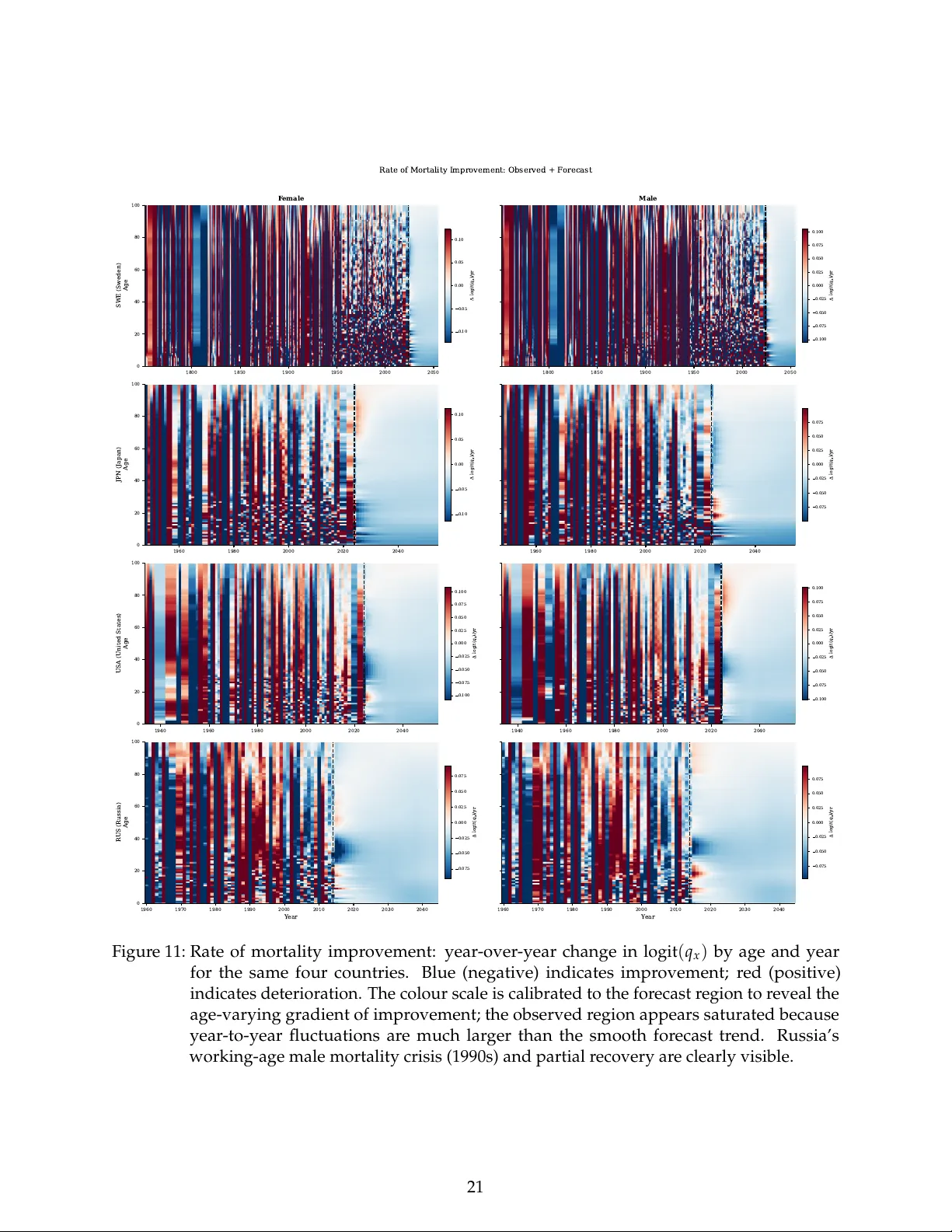
Mortality Forecasting as a Flow Field in T ucker Decomposition Space Samuel J. Clark Department of Sociology , The Ohio State University 2026 W e intr oduce a mortality for ecasting method that r eframes the pr oblem as integrating a ﬂow ﬁeld through a low-dimensional space derived from the T ucker decomposition of multi-population mortality data. The T ucker decomposition of the Human Mortality Database’s sex–age–country–year tensor provides a compact repr esentation in which every country-year ’s complete mortality schedule is determined by a small effective core matrix G ct . PCA reduction of the vectorised G ct reveals that ﬁve components capture 97% of the variance, with the ﬁrst component alone accounting for 92% – the mortality level. The derivatives of all ﬁve components are tightly correlated (e.g. Corr ( ∆ s 1 , ∆ s 2 ) = − 0.92), revealing that the mortality transition is essentially a one- dimensional ﬂow through 5D scor e space. The forecaster navigates directly in score space: a speed function g ∗ ( s 1 ) = d s 1 / d t advances th e level scor e, while trajectory functions f ∗ k ( s 1 ) map the level to the str uctural scores for k = 2, . . . , 5. Life expectancy e 0 is computed fr om the T ucker-r econstructed mortality surface at each forecast horizon. An era-weighted speed function with a truncated exponential kernel gives more weight to contemporary dynamics at each forecast origin, avoiding the bias fr om averaging over disparate eras of the mortality transition. Structural score deviations r elax toward the HMD-wide canonical pattern at empirically calibrated rates (half-lives 12–32 years). In leave-country-out cr oss-validation (48 held-out countries, 50-year horizon, 9,529 test points), the system achieves e 0 MAE of 4.46 years – 19% below Lee–Carter (5.53 years) and 23% below Hyndman–Ullah (5.76 years). At short horizons ( h = 1– 10), Lee–Carter and Hyndman–Ullah are more accurate; the ﬂow-ﬁeld advantage emerges at h ≈ 12 and grows to 36–41% at horizons of 26–50 years. Critically , the ﬂow-ﬁeld has near -zero aggr egate bias ( − 0.05 years), while Lee–Carter ( − 4.33 years) and Hyndman–Ullah ( − 4.67 years) systematically underpredict futur e life expectancy . 1 Contents 1 Introduction 3 2 T ucker Decomposition 4 3 The Flow Field 5 3.1 PCA reduction . . . . . . . . . . . . . . . . . . . . . . . . . . . . . . . . . . . . . . . . . 5 3.2 One-dimensional dynamics . . . . . . . . . . . . . . . . . . . . . . . . . . . . . . . . . 5 3.3 Speed function and trajectory functions . . . . . . . . . . . . . . . . . . . . . . . . . . 6 4 Forecasting Architecture 7 4.1 Era-weighted speed function . . . . . . . . . . . . . . . . . . . . . . . . . . . . . . . . 7 4.2 Score-space navigation . . . . . . . . . . . . . . . . . . . . . . . . . . . . . . . . . . . . 8 4.3 Speed dynamics . . . . . . . . . . . . . . . . . . . . . . . . . . . . . . . . . . . . . . . . 9 4.4 Score r elaxation . . . . . . . . . . . . . . . . . . . . . . . . . . . . . . . . . . . . . . . . 9 4.5 T ucker reconstruction and e 0 computation . . . . . . . . . . . . . . . . . . . . . . . . . 10 4.6 T rajectory extrapolation beyond observed data . . . . . . . . . . . . . . . . . . . . . . 10 4.7 Prediction intervals . . . . . . . . . . . . . . . . . . . . . . . . . . . . . . . . . . . . . . 12 4.8 Empirical convergence rates . . . . . . . . . . . . . . . . . . . . . . . . . . . . . . . . . 13 5 Cross-V alidation Results 14 5.1 Benchmark comparison . . . . . . . . . . . . . . . . . . . . . . . . . . . . . . . . . . . 15 5.2 Leave-country-out holdout gallery . . . . . . . . . . . . . . . . . . . . . . . . . . . . . 16 5.3 Accuracy by horizon . . . . . . . . . . . . . . . . . . . . . . . . . . . . . . . . . . . . . 16 5.4 Prediction interval calibration . . . . . . . . . . . . . . . . . . . . . . . . . . . . . . . . 18 5.5 Sex-age coherence and smooth jump-of f . . . . . . . . . . . . . . . . . . . . . . . . . . 19 5.6 Sex differ ential coher ence . . . . . . . . . . . . . . . . . . . . . . . . . . . . . . . . . . 22 6 Application to Non-HMD Populations 22 7 Discussion 26 7.1 Parsimony . . . . . . . . . . . . . . . . . . . . . . . . . . . . . . . . . . . . . . . . . . . 27 7.2 Integrated framework . . . . . . . . . . . . . . . . . . . . . . . . . . . . . . . . . . . . 27 7.3 Structural sex-age coher ence . . . . . . . . . . . . . . . . . . . . . . . . . . . . . . . . . 27 7.4 Complete sex-speciﬁc mortality schedules . . . . . . . . . . . . . . . . . . . . . . . . . 28 7.5 Long-horizon accuracy and systematic bias . . . . . . . . . . . . . . . . . . . . . . . . 28 7.6 Applicability beyond the HMD . . . . . . . . . . . . . . . . . . . . . . . . . . . . . . . 29 7.7 Model life table system as byproduct . . . . . . . . . . . . . . . . . . . . . . . . . . . . 29 7.8 Suggestive trajectory behavior at very low mortality levels: a lifespan limit? . . . . . 30 7.9 Limitations and extensions . . . . . . . . . . . . . . . . . . . . . . . . . . . . . . . . . . 31 2 8 Computational Environment and Acknowledgements 33 9 Notation 34 References 36 1 Introduction The dominant paradigm for mortality forecasting since Lee and Carter ( 1992 ) is to decompose age-speciﬁc mortality rates via the singular value decomposition, then extrapolate the temporal component(s) using time series models – typically a random walk with drift. Extensions increase the SVD rank ( Booth et al. , 2002 ; Hyndman and Ullah , 2007 ), add coherent multi-population structur e ( Li and Lee , 2005 ; Hyndman et al. , 2013 ), model the rotation of age patterns ( Li et al. , 2013 ), or use mor e sophisticated time series models ( de Jong and T ickle , 2006 ). Evaluations ( Lee and Miller , 2001 ; Booth et al. , 2006 ) and recent reviews ( Booth and T ickle , 2008 ; Basellini et al. , 2023 ) document persistent challenges: the ﬁxed age pattern in Lee–Carter underpredicts life expectancy , independent sex-speciﬁc ﬁts produce diver gent forecasts, and prediction intervals ar e sensitive to model choice. A complementary tradition models life expectancy gains as a function of the current mortality level. Raftery et al. ( 2013 ) introduced a Bayesian hierarchical model in which ﬁve-year gains in e 0 follow a double-logistic function of e 0 , with country-speciﬁc parameters drawn from a world distribution. This approach – now the basis of the United Nations’ ofﬁcial population projections – captures the empirically observed pattern ( Oeppen and V aupel , 2002 ) in which the rate of mortality improvement depends on where a country sits in the epidemiological transition rather than on calendar time. However , it for ecasts only the scalar e 0 ; converting the pr ojected e 0 to age-speciﬁc rates requir es a separate model life table system. T ensor decomposition methods extend the Lee–Carter approach to multi-way data. Russolillo et al. ( 2011 ) applied a rank-2 T ucker decomposition to 10 European populations, and Dong et al. ( 2020 ) compared canonical polyadic and T ucker decompositions for multi-population forecasting, in both cases extrapolating the time-mode factor vectors via ARIMA. Zhang et al. ( 2023 ) developed adaptive penalised tensor decomposition for cause-of-death mortality . This paper uniﬁes these two traditions. The T ucker decomposition of the Human Mortality Database’s mortality tensor – developed as part of the MDMx system ( Clark , 2026 ) – provides a structur ed low-dimensional space in which every country-year is represented by a point. W e show that the dynamics in this space are remarkably simple: the derivatives of all ﬁve PCA components of the effective core matrix G ct are tightly correlated ( r = − 0.92 for the ﬁrst two components), revealing that the mortality transition is essentially a one-dimensional ﬂow . Forecasting r educes to 3 learning a scalar speed function g ∗ ( s 1 ) = d s 1 / d t and trajectory functions f ∗ k ( s 1 ) for k = 2, . . . , 5 that map the level score to the structural scores – from which the complete sex-speciﬁc, single- year-of-age mortality schedule is r econstructed via the T ucker basis matrices. Life expectancy e 0 is computed from the r econstructed mortality surface at each horizon for reporting only , avoiding the systematic bias that arises when an e 0 accumulator diverges fr om the surface-derived e 0 through the nonlinear expit/life-table chain. The conceptual reframing is fr om “project the time index forward” (Lee–Carter and extensions) to “the mortality transition is a ﬂow through a structur ed space, parameterised by level” (the present approach). The speed function is the T ucker-space analogue of the Raftery et al. level-dependent improvement rate, and the trajectory functions ar e a continuous model life table system in T ucker coordinates – but unlike the WPP pipeline, the forecasting model and the reconstr uction model are uniﬁed in a single framework, and the navigation coordinate is the PCA level score rather than the scalar e 0 . Three additional innovations shape the production system. First, an era-weighted speed func- tion uses a truncated exponential kernel centred on each forecast origin, giving more weight to contemporary dynamics and avoiding the bias that arises fr om averaging over disparate eras of the mortality transition. Second, empirically calibrated convergence rates – measured from the observed autocorr elation of country-level deviations fr om canonical dynamics – contr ol how quickly each country’s distinctive mortality structure relaxes toward the HMD-wide canonical pattern; structural score deviations persist for 12–32 years. Third, the optimal speed blend weight is w = 1.0 (fully canonical), though the MAE varies by only a few hundredths of a year across the full range of w : the forecast reduces to a deterministic integration along a curve in T ucker PCA space. W e evaluate the system using leave-country-out cr oss-validation with a 50-year for ecast horizon – dir ectly testing the pr oduction use case of forecasting a country whose data did not contribute to the ﬂow ﬁeld. The system achieves e 0 MAE of 4.46 years (19% below Lee–Carter , 23% below Hyndman–Ullah), with the advantage concentrated at long horizons (36–41% at h = 26–50). More importantly , the ﬂow-ﬁeld has near-zer o aggregate bias ( − 0.05 years) while Lee–Carter and Hyndman–Ullah systematically underpredict life expectancy by over four years – the critical distinction for long-range population projections, pension planning, and actuarial applications. 2 T ucker Decomposition W e work with the rank- ( r 1 , r 2 , r 3 , r 4 ) T ucker decomposition of the logit ( q x ) mortality tensor M ∈ R S × A × C × T ( S = 2 sexes, A = 110 ages, C = 48 countries, T = 274 years) from the HMD, as developed in Clark ( 2026 ). The decomposition pr oduces factor matrices S ∈ R S × r 1 (sex), A ∈ R A × r 2 (age), C ∈ R C × r 3 (country), T ∈ R T × r 4 (year), and a cor e tensor G ∈ R r 1 × r 2 × r 3 × r 4 with ranks ( 2, 42, 46, 100 ) . 4 Every country-year ’s mortality schedule is determined by the effective cor e matrix G ct [ i , j ] = ∑ k , l G [ i , j , k , l ] C [ c , k ] T [ t , l ] , (1) and the reconstruction is ˆ M :,: , c , t = S G ct A ⊤ . The r 1 × r 2 = 84 elements of G ct are the forecasting target. 3 The Flow Field 3.1 PCA reduction PCA on all observed vec ( G ct ) vectors shows that ﬁve components captur e 97.1% of the total variance (table 1 ), with the ﬁrst component alone accounting for 91.8% – it is the mortality level. T able 1: PCA of vec ( G ct ) : variance explained. Component V ariance Cumulative PC 1 91.8% 91.8% PC 2 2.6% 94.4% PC 3 1.5% 95.9% PC 4 0.7% 96.7% PC 5 0.4% 97.1% 3.2 One-dimensional dynamics Smoothing each country’s PCA score trajectory (LOWESS, fraction 0.25) and differ entiating reveals that the derivative vector is essentially one-dimensional. Using raw forward dif ferences – which preserve the shar ed transient shocks (wars, pandemics, economic crises) that simultaneously push multiple PCA components – the correlations between ∆ s 1 (rate of level change) and the structural derivatives are: Pair Correlation ∆ s 1 , ∆ s 2 − 0.922 ∆ s 1 , ∆ s 3 − 0.548 ∆ s 1 , ∆ s 4 + 0.496 ∆ s 1 , ∆ s 5 + 0.571 5 The interpr etation: when countries move thr ough the mortality transition, all ﬁve PCA components move in lockstep. The trajectory has a shape (the curve thr ough 5D score space) and a speed (how fast a country traverses it), and these ar e nearly separable. The entire 5D trajectory – encoding 84 T ucker weights and hence 220 logit ( q x ) values – is to close approximation a function of a single scalar: the level score s 1 (equivalently , e 0 ). Figure 1 visualises this structur e. The top-left panel shows the raw year-to-year e 0 velocity (for- ward differ ences) as a function of mortality level – the same raw data used in the derivative correlation panels. The scatter is noisy because raw forward dif ferences include wars, pandemics, and stochastic year-to-year ﬂu ctuation, but the LOWESS trend r eveals the broad level-dependent pattern: improvement is concentrated at intermediate e 0 levels and decelerates at the frontier . The production speed function (section 3.3 ) uses per -country smoothed velocities that ﬁlter this noise, revealing a cleaner proﬁle inspired by but more complex than the parametric double-logistic of Raftery et al. ( 2013 ) – the nonparametric LOWESS captures empirical structure, including asymme- try and plateau regions, that a parametric form would impose away . The top-centre and top-right panels show the derivative corr elations ∆ s 1 vs ∆ s 2 and ∆ s 3 : the tight linear relationship ( r = − 0.92) demonstrates that the 5D dynamics compress into a one-dimensional ﬂow . The bottom panels show the canonical trajectories: each PCA score traces a tight curve as a function of e 0 (equivalently , of s 1 ), with individual countries scattered ar ound the LOWESS trend. 3.3 Speed function and trajectory functions Since s 1 is approximately the mortality level, the ﬂow ﬁeld is deﬁned in s 1 space rather than e 0 space. The speed function g ∗ ( s 1 ) = d s 1 / d t is estimated by LOWESS r egression of the smoothed s 1 velocity (forward dif ferences of per-country LOWESS-smoothed s 1 ) on s 1 across all country-years in the training set. The trajectory functions f ∗ k ( s 1 ) for k = 2, . . . , 5 are LOWESS regr essions of each raw PCA score on raw s 1 . T ogether , they encode the canonical sex-age mortality pattern at each mortality level – a continuous model life table system in T ucker coor dinates, parameterised by the level score. The smoothing pipeline for the speed function is designed to separate signal fr om noise: per- country LOWESS denoises year-to-year ﬂuctuations (wars, pandemics, economic shocks) while preserving the underlying improvement trend; forward differ ences match the forecaster ’s one- step-ahead model; and the cr oss-country LOWESS extracts the level-dependent pattern fr om the pooled observations. The resulting speed proﬁle (ﬁg. 2 ) is inspir ed by the level-dependent pattern of Raftery et al. ( 2013 ) – improvement concentrated at intermediate mortality levels, decelerating at the frontier – but the nonparametric estimation r eveals empirical structure, including asymmetry and plateau regions, that a parametric double-logistic would impose away . Operating in score space eliminates the nonlinear mapping between the navigation coordinate and the reported e 0 (section 4.2 ). 6 20 30 40 50 60 70 80 90 e 0 1.5 1.0 0.5 0.0 0.5 1.0 1.5 d e 0 / d t ( y e a r s / y e a r ) S p e e d F u n c t i o n g ( e 0 ) LOWES S 10 5 0 5 10 s 1 3 2 1 0 1 2 3 s 2 r ( s 1 , s 2 ) = 0 . 9 2 2 10 5 0 5 10 s 1 2.0 1.5 1.0 0.5 0.0 0.5 1.0 1.5 2.0 s 3 r ( s 1 , s 3 ) = 0 . 5 4 8 0 20 40 60 80 e 0 20 0 20 40 60 80 s 1 T r a j e c t o r y : s 1 = f 1 ( e 0 ) f 1 ( e 0 ) 0 20 40 60 80 e 0 15 10 5 0 5 s 2 T r a j e c t o r y : s 2 = f 2 ( e 0 ) f 2 ( e 0 ) 0 20 40 60 80 e 0 10 8 6 4 2 0 2 4 s 3 T r a j e c t o r y : s 3 = f 3 ( e 0 ) f 3 ( e 0 ) Flow-Field Structure in Tucker PCA Space Figure 1: Flow-ﬁeld structur e in T ucker PCA space. T op left: raw year-to-year e 0 velocity (forward differ ences) vs e 0 – the scatter is noisy but the LOWESS trend reveals level-dependent improvement; the pr oduction speed function uses per-country smoothed velocities in s 1 space for a cleaner estimate (ﬁg. 2 ). T op centr e and right: derivative correlations ∆ s 1 vs ∆ s 2 and ∆ s 3 (raw forward dif ferences); the tight linear r elationship ( r = − 0.92) demonstrates one-dimensional dynamics. Bottom: canonical trajectories s k vs e 0 for PCs 1–3 – each score is a tight function of mortality level, comprising a continuous model life table system in T ucker coordinates. 4 Forecasting Architecture 4.1 Era-weighted speed function The canonical speed function g ∗ ( s 1 ) averages over the entire historical recor d – Sweden in 1860 and Japan in 2010 contribute equally . But the pace of mortality improvement at a given level has changed through time: the rapid gains of the mid-20th century epidemiological transition are not repr esentative of contemporary dynamics at the same mortality levels. A speed function trained on all eras systematically overpr edicts impr ovement because it includes the fast-impr ovement decades alongside the recent deceleration. W e address this with a truncated exponential weighting kernel applied to the LOWESS training 7 20 10 0 10 20 s 1 ( s m o o t h e d ) 1.25 1.00 0.75 0.50 0.25 0.00 0.25 0.50 0.75 d s 1 / d t A: Smoothed fwd diffs LOWES S (A) 20 0 20 40 60 80 s 1 ( r a w ) 60 40 20 0 20 40 d s 1 / d t B: R aw fwd diffs LOWES S (B) 20 0 20 40 60 80 s 1 50 40 30 20 10 0 d s 1 / d t Comparison A: Smoothed B: R aw S p e e d F u n c t i o n i n s 1 S p a c e : P e r - C o u n t r y S m o o t h i n g v s R a w P o o l i n g Figure 2: Speed function denoising comparison in s 1 space. Left: per-country LOWESS-smoothed forward differ ences pooled across countries (Method A, production) – the smoothing reveals the underlying improvement trend. Centr e: raw forward differences pooled directly (Method B) – the cross-country LOWESS alone cannot fully denoise the year- to-year noise. Right: overlay of the two LOWESS estimates, showing that per-country smoothing is essential for a well-behaved speed function. data. Given a forecast origin at calendar year t 0 , each observation at year t receives weight w era ( t ) =    exp  − ( t 0 − t ) · ln 2 / τ  if t 0 − t ≤ W 0 otherwise (2) where τ is the half-life of the exponential decay and W is a hard window beyond which data is discarded entirely . At τ = 20 and W = 40: data from 20 years befor e the origin r eceives half weight; data from 40 years befor e receives one-quarter weight; older data is excluded. This is applied only to the speed function, not to the trajectory functions f ∗ k ( s 1 ) – the canonical sex-age mortality patterns are structural features of the mortality transition that change slowly , while the pace at which countries traverse the transition is era-dependent. Cross-validation over τ ∈ { 10, 12, 15, 20, 30 } ﬁnds the optimum at τ = 12 (section 5 ). 4.2 Score-space navigation A natural approach would navigate in e 0 space: accumulate e 0 ( h ) = e 0 ( h − 1 ) + g ( e 0 ( h − 1 ) ) , look up canonical scores at the current e 0 , reconstruct the mortality surface, and report the surface- derived e 0 . However , this creates two distinct e 0 values at each horizon: the navigation e 0 (the scalar accumulator) and the surface e 0 (computed from the T ucker reconstruction thr ough the nonlinear expit and life-table chain). These diverge systematically because the trajectory functions f k ( e 0 ) are smoothed independently , the expit transform is concave in the relevant range, and the life-table calculation is nonlinear in q x . In cross-validation, e 0 -space navigation pr oduces a persistent negative bias of ∼ 1.6 years. 8 The solution is to navigate in score space dir ectly . Since s 1 ≈ level , we deﬁne the speed function as g ∗ ( s 1 ) = d s 1 / d t and the trajectory functions as f ∗ k ( s 1 ) for k = 2, . . . , 5. The forecast advances s 1 at each step; the trajectory functions map s 1 to the structural scor es; the T ucker r econstruction produces the mortality surface; and e 0 is computed fr om this surface for r eporting. Because s 1 is the ﬁrst coordinate of the reconstr ucted score vector – not a separate accumulator – there is no divergence between the navigation variable and the r econstruction. The nonlinear expit/life-table mapping is applied once, at the end, to compute the reported e 0 – it never feeds back into the navigation loop. 4.3 Speed dynamics The forecast advances s 1 at each step using a hierarchical blend of the era-weighted canonical speed and the country’s own recent s 1 velocity , with empirical relaxation from country-speciﬁc to canonical dynamics: v s 1 ( h ) =  w + ( 1 − w ) ( 1 − α h v )  · g ∗ τ  s 1 ( h − 1 )  + ( 1 − w ) · α h v · v s 1 ,country , (3) s 1 ( h ) = s 1 ( h − 1 ) + v s 1 ( h ) , (4) where g ∗ τ is the era-weighted speed function in s 1 space, v s 1 ,country is the country’s trailing-mean s 1 velocity at the forecast origin (mean of the last 5 raw forward dif ferences), α v is the empirical speed relaxation rate (section 4.8 ), and w ∈ [ 0, 1 ] is the speed blend weight. Cross-validation ﬁnds the optimal blend weight at w = 1.0 (fully canonical), though the MAE varies by only a few hundredths of a year across the full range of w . At w = 1, eq. ( 3 ) simpliﬁes to v s 1 ( h ) = g ∗ τ ( s 1 ( h − 1 ) ) and the forecast r educes to a deterministic integration along a curve in T ucker PCA space. 4.4 Score relaxation The level scor e s 1 is the navigation variable – it is advanced by the speed function (eq. ( 4 )) and is not relaxed. The structural scores s k for k = 2, . . . , 5 relax from the country’s actual curr ent value toward the canonical trajectory: s k ( h ) = α h s , k · s actual k + ( 1 − α h s , k ) · f ∗ k  s 1 ( h )  , k = 2, . . . , 5 , (5) where α s , k ∈ [ 0, 1 ) is the per -component relaxation rate, calibrated empirically fr om the observed autocorrelation of score deviations (section 4.8 ). The structural components have half-lives of 12–32 years (PC 2: 32 yr , PC 3: 30 yr , PC 4: 12 yr , PC 5: 29 yr). 9 The relaxation gives the forecast memory of the country’s current deviation from the canonical sex-age structure. A country whose age pattern differs fr om the HMD average at its mortality level – for example, Eastern European countries with excess working-age male mortality – will retain that distinctive structure for decades (consistent with the 12–32 year empirical half-lives) and gradually converge towar d the canonical trajectory . 4.5 T ucker reconstruction and e 0 computation At each horizon h , the forecast score vector s ( h ) = ( s 1 ( h ) , s 2 ( h ) , . . . , s 5 ( h ) ) – where s 1 ( h ) comes from the speed function and s 2 , . . . , s 5 from scor e relaxation – is mapped back to the full logit ( q x ) schedule: ˆ M :,: ( h ) = S  ¯ g + s ( h ) · V  reshaped A ⊤ , (6) where V contains the PCA loadings and ¯ g is the mean vec ( G ct ) . Because the reconstr uction uses the shared factor matrices S and A , the resulting female and male schedules are str ucturally coherent by construction. Life expectancy e 0 is then computed from the reconstructed schedule through the standard expit and life-table chain – this is the only point at which the nonlinear logit ( q x ) → q x → e 0 mapping is applied, and its output is never fed back into the navigation. The ﬁve-component PCA captures 97.1% of the variance in vec ( G ct ) , but the remaining 2.9% includes country-speciﬁc sex-differ ential structur e – particularly for countries whose sex gap deviates substantially from the HMD average (e.g. Russia, Japan). T o avoid a visible discontinuity in the sex differ ential at the forecast origin, the for ecast surface incorporates a jump-off correction : the residual between the full-rank T ucker reconstruction ˆ M :,: , c , T and its ﬁve-component approximation is added to the forecast surface and decayed exponentially with a half-life of 2 years: ˆ M :,: ( h ) = S  ¯ g + s ( h ) · V  reshaped A ⊤ + 2 − h / 2 · ∆ 0 , (7) where ∆ 0 = ˆ M :,: , c , T − S ( ¯ g + s T · V ) reshaped A ⊤ is the origin residual. By h = 2 the correction has halved; by h = 10 it is below 4%; and the long-horizon forecast is determined entir ely by the ﬁve- component dynamics. The short half-life allows the ﬁve-component dynamics to take ef fect quickly while smoothing the sex-differ ential transition at the origin – without the jump-off corr ection, the 2.9% of variance not captured by the 5-PC approximation would produce a visible discontinuity in the sex gap at the forecast origin. 4.6 T rajectory extrapolation beyond observed data The trajectory functions f ∗ k ( s 1 ) and speed function g ∗ ( s 1 ) are LOWESS ﬁts to observed HMD data. In s 1 space, the mortality frontier is at low s 1 values (corresponding to high e 0 ≈ 85, primarily Japan). Beyond the observed range, the LOWESS interpolant holds each function constant at 10 its boundary value – the structural scor es stop evolving and the reconstructed mortality surface saturates. Fix: joint tangent extension. At a transition point s ∗ 1 ≈ − 12 (the s 1 value corresponding to e 0 ≈ 78, well inside the observed range), the LOWESS slope of each function is estimated via ﬁnite differ ences. These slopes form a joint tangent vector – the empirical direction of score-space movement at the mortality frontier . Beyond the transition, the LOWESS values are replaced by linear extrapolation along this tangent, with a smooth-step blend: f ∗ k ( s 1 ) =            f ∗ ,LOWESS k ( s 1 ) if s 1 ≥ s ∗ 1 blend of LOWESS and linear if s ∗ 1 − 3 ≤ s 1 < s ∗ 1 f ∗ k ( s ∗ 1 ) + t k ( s 1 − s ∗ 1 ) if s 1 < s ∗ 1 − 3 (8) where t k is the LOWESS slope at s ∗ 1 . The same treatment is applied to the speed function. Because all slopes come from the same s 1 region, the joint covariance of the scor e trajectories is preserved – all components continue to move in the direction established by the well-observed interior data. Figure 3 shows the s 1 -to-surface- e 0 mapping with and without the tail extension. Figure 4 validates the tangent direction by comparing it to the actual direction of score movement in the ﬁve highest- e 0 countries (Japan, Sweden, Switzerland, Spain, Italy) over their most r ecent 20 years. Figure 5 shows the resulting forecast e 0 trajectories for six countries – because the system navigates in s 1 space, there is no separate navigation e 0 that can diverge fr om the surface e 0 . 40 20 0 20 40 60 80 s 1 ( P C 1 ) 0 20 40 60 80 Surface e (life table) R aw LOWES S (flat extrapolation) Both (raw) F emale (raw) Male (raw) 40 20 0 20 40 60 80 s 1 ( P C 1 ) 0 20 40 60 80 Surface e (life table) Joint tangent extension Both (extended) F emale (extended) Male (extended) Transition s =-12.2 s 1 S u r f a c e e M a p p i n g ( P C 1 - s p a c e n a v i g a t i o n ) Figure 3: s 1 -to-surface- e 0 mapping. Left: raw LOWESS with ﬂat extrapolation – surface e 0 saturates at the frontier . Right: with joint tangent extension from s ∗ 1 ≈ − 12 ( e 0 ≈ 78) – surface e 0 continues to improve monotonically . Pink: female; cyan: male; green: both-sex average. 11 PC2 PC3 PC4 PC5 1.25 1.00 0.75 0.50 0.25 0.00 0.25 0.50 0.75 d s k / d s 1 Frontier-Country T angent V alidation (s space) LOWES S tangent JPN SWE CHE ESP IT A Frontier avg Figure 4: V alidation of the joint tangent extrapolation in s 1 space. Per -component score slopes d s k / d s 1 for the LOWESS tangent at s ∗ 1 ≈ − 12 ( e 0 ≈ 78, red) and for ﬁve frontier countries (Japan, Sweden, Switzerland, Spain, Italy) over their last 20 years. The cosine similarity between the LOWESS tangent and the frontier average is 0.94, conﬁrming that the extrap- olation direction agrees with observed frontier dynamics. The magnitude ratio is 0.59 – the tangent extrapolation is ∼ 40% conservative in speed r elative to frontier countries, producing a modestly cautious long-horizon for ecast. 4.7 Prediction intervals The forecast uncertainty is estimated empirically from the cr oss-validation error distribution. A horizon-dependent bias correction b ( h ) , estimated by LOWESS regression of the CV errors on horizon, is subtracted from the raw forecast; the corr ected forecast is ˆ e 0 ( h ) − b ( h ) . W e model the residual uncertainty as σ ( h ) = κ · σ 1 · √ h , the natural scaling for accumulated random-walk- like forecast err ors, where σ 1 is the median of the per-horizon empirical standar d deviations divided by √ h , and κ = SD ( z -scores ) calibrates the coverage. The 95% pr ediction interval is ˆ e 0 ( h ) − b ( h ) ± 1.96 · σ ( h ) . 12 1750 1800 1850 1900 1950 2000 2050 Y ear 20 30 40 50 60 70 80 90 e e (h=30) = +3.7 SWE (e =83.5) Observed Surface e (raw) Surface e b(h) Surface F Surface M 1960 1980 2000 2020 2040 2060 2080 Y ear 50 60 70 80 90 e e (h=30) = +3.3 JPN (e =83.6) Observed Surface e (raw) Surface e b(h) Surface F Surface M 1940 1960 1980 2000 2020 2040 2060 2080 Y ear 60 65 70 75 80 85 90 e e (h=30) = +3.9 USA (e =79.0) Observed Surface e (raw) Surface e b(h) Surface F Surface M 1960 1980 2000 2020 2040 2060 Y ear 65 70 75 80 e e (h=30) = +5.9 RUS (e =70.4) Observed Surface e (raw) Surface e b(h) Surface F Surface M 1960 1980 2000 2020 2040 2060 Y ear 70 75 80 85 90 e e (h=30) = +4.9 POL (e =80.6) Observed Surface e (raw) Surface e b(h) Surface F Surface M 1900 1925 1950 1975 2000 2025 2050 2075 Y ear 20 30 40 50 60 70 80 90 e e (h=30) = +3.8 ESP (e =83.5) Observed Surface e (raw) Surface e b(h) Surface F Surface M F orecast e Diagnostic (PC1-space navigation) Figure 5: Forecast e 0 diagnostic for six countries under s 1 -space navigation (all-data ﬂow ﬁeld). Green: surface-derived e 0 (raw , before bias corr ection). Red dash-dot: bias-corrected e 0 (reported for ecast). The annotation shows the 30-year e 0 gain. Because navigation is in s 1 space, there is no separate navigation e 0 that can diverge fr om the surface e 0 . 4.8 Empirical convergence rates The relaxation rates α in eqs. ( 3 ) and ( 5 ) can be calibrated empirically rather than tuned by forecast accuracy . For each country-year we compute the deviation fr om canonical: ∆ v s 1 ( t ) = v s 1 ,country ( t ) − g ∗ ( s 1 ( t ) ) for speed, and ∆ s k ( t ) = s k ( t ) − f ∗ k ( s 1 ( t ) ) for each structural score ( k = 2, . . . , 5; PC 1 deviations are identically zero by construction since s 1 is the navigation variable). The pooled autocorrelation at lag h – β ( h ) = ∑ c , t 0 ∆ ( t 0 + h ) · ∆ ( t 0 ) ∑ c , t 0 ∆ ( t 0 ) 2 – measures how much of a deviation persists h years later . If convergence is exponential, β ( h ) = α h and the ﬁtted slope of log β vs. h gives α directly . Figure 6 shows that structural score deviations ar e persistent: PCs 2–5 have half-lives of 12–32 years, conﬁrming that a country’s mortality pattern is deeply entr enched. These empirical rates are used directly in the pr oduction forecaster . Because w = 1.0 (fully canonical speed), the speed relaxation rate α v does not af fect the forecast – the system uses canonical speed at every horizon. The cross- 13 validation (section 5 ) additionally selects the era half-life τ from a coarse grid; the MAE varies by only a few hundredths of a year acr oss the full range of w . 0 5 10 15 20 25 30 L a g h ( y e a r s ) 0.2 0.0 0.2 0.4 0.6 0.8 1.0 A u t o c o r r e l a t i o n ( h ) 1 (non-convergent; irrelevant at w=1) Speed deviations (s space) Speed ( =1.028) 0 5 10 15 20 25 30 L a g h ( y e a r s ) 0.0 0.2 0.4 0.6 0.8 1.0 A u t o c o r r e l a t i o n ( h ) Score deviations by PC PC 1 ( =n/a) PC 2 ( =0.979) PC 3 ( =0.977) PC 4 ( =0.946) PC 5 ( =0.976) 0 5 10 15 20 25 30 L a g h ( y e a r s ) 0.2 0.0 0.2 0.4 0.6 0.8 1.0 A u t o c o r r e l a t i o n ( h ) S p e e d : l o w v s h i g h e 0 e 0 < 7 2 . 0 ( = 1 . 0 1 3 ) e 0 7 2 . 0 ( = 1 . 0 1 1 ) Empirical Convergence to Canonical Dynamics Figure 6: Empirical convergence rates in s 1 space. Left: autocorrelation of s 1 -velocity deviations from canonical. Centre: autocorrelation of structural score deviations by PC; PCs 2–5 have half-lives of 12–32 years. Right: speed convergence conditioned on mortality level. Dashed lines show ﬁtted exponentials α h . 5 Cross-V alidation Results The system is evaluated by leave-country-out cross-validation: for each of the 48 HMD countries in turn, the ﬂow ﬁeld is built from the r emaining 47 countries using all available years, then applied to the held-out country at multiple forecast origins (every 10 years, r equiring at least 20 training years), with for ecasts extending up to 50 years. This produces 9,529 test points and directly tests the production use case: can HMD-wide dynamics predict a country whose data did not train the ﬂow ﬁeld? The 50-year horizon is essential – mortality for ecasting routinely r equir es 50–75 year projections (the UN WPP projects to 2100; the US Social Security Administration uses 75-year horizons) – and the ﬂow-ﬁeld system’s constrained dynamics provide a distinctive advantage at these horizons. The cross-validation proceeds in two stages. First, a fast grid search over the era half-life τ and speed blend weight w uses inclusive ﬂows (built from all 48 countries) to identify the optimal conﬁguration – this is computationally efﬁcient because the ﬂows need not be rebuilt for each held-out country . Second, the optimal conﬁguration is evaluated under strict leave-country-out: for each held-out country , the ﬂow ﬁeld is r ebuilt from the remaining 47 countries, ensuring that the held-out country’s data contributes nothing to the speed function, trajectory functions, or era weighting. All MAE, bias, and coverage statistics reported in this paper are from the strict leave-country-out evaluation – the gold standard for out-of-sample for ecast assessment. A note on bias measures. The pr oduction for ecasts and diagnostic ﬁgures (ﬁgs. 5 , 16 and 17 ) use the 14 all-data ﬂow ﬁeld (all 48 countries), which introduces a small upwar d bias ( ∼ 1 year) because each country’s own dynamics ar e reﬂected in the canonical ﬂow . The strict leave-country-out bias – in which the held-out country’s data is genuinely excluded from the ﬂow – is near zero ( − 0.05 years), conﬁrming that the s 1 -space navigation ar chitecture is unbiased in the out-of-sample setting that matters for production for ecasting. The fast grid search (Stage 1) optimises jointly over the era half-life τ ∈ { 10, 12, 15, 20, 30 } and the speed blend weight w ∈ { 0.2, 0.5, 1.0 } . The optimal conﬁguration is τ = 12, w = 1.0 – that is, fully canonical speed with the selected era half-life. The speed blend weight barely matters – MAE varies by only a few hundredths of a year across w ∈ [ 0.2, 1.0 ] – conﬁrming that the era-weighted canonical dynamics, not the country-speciﬁc velocity , drive forecast quality . The strict leave-country-out evaluation (Stage 2) then uses this optimal conﬁguration to produce the r esults reported below . 5.1 Benchmark comparison T able 2 compares the ﬂow-ﬁeld system against Lee–Carter ( Lee and Carter , 1992 ) and Hyndman– Ullah ( Hyndman and Ullah , 2007 ), computed using the R demography package with HMD grad- uated m x and person-year exposur es: Lee–Carter uses lca(adjust="none") with ﬁtted jump-of f rates; Hyndman–Ullah uses fdm(order=6) with ARIMA extrapolation of each score. All three methods are evaluated on the same 9,529 test points using the same e 0 computation. T able 2: Benchmark comparison: leave-country-out CV (50-year horizon). Method n MAE RMSE Bias Flow-ﬁeld 9529 4.459 7.265 -0.049 LC 9529 5.528 7.934 -4.334 HU 9529 5.761 8.327 -4.667 The ﬂow-ﬁeld system achieves an e 0 MAE of 4.46 years, 19% below Lee–Carter (5.53 years) and 23% below Hyndman–Ullah (5.76 years), with near-zer o aggregate bias ( − 0.05 years in strict leave- country-out evaluation). The horizon proﬁle is the central result (ﬁg. 7 ): at short horizons ( h = 1–10), Lee–Carter and Hyndman–Ullah are more accurate (MAE 2.8–3.4 vs 3.7–3.9 for the ﬂow-ﬁeld), because their proper jump-of f adjustment and ARIMA score extrapolation captur e recent momen- tum more effectively . The crossover occurs at h ≈ 12, and by h = 16–25 the ﬂow-ﬁeld leads by 11–15%. At h = 26–50, the advantage reaches 36–41%: the ﬂow-ﬁeld achieves MAE 5.2 years while Lee–Carter reaches 8.1 and Hyndman–Ullah 8.8, because their linear extrapolation accumulates systematic underprediction while the ﬂow-ﬁeld is constrained to the canonical trajectory . 15 0 1 2 3 4 5 6 MAE (years) Flow-field LC HU 4.46 (bias=-0.05) 5.53 (bias=-4.33) 5.76 (bias=-4.67) Overall MAE 1 5 6 15 16 25 26 50 Horizon band 0 2 4 6 8 MAE (years) MAE by Horizon Band Flow-field LC HU 0 10 20 30 40 50 Horizon (years) 2 4 6 8 10 12 MAE (years) MAE by Horizon Flow-field LC HU Flow-Field vs Lee-Carter vs Hyndman-Ullah Figure 7: Benchmark comparison across 9,529 strict leave-country-out CV test points (each country’s ﬂow built excluding that country). Lee–Carter and Hyndman–Ullah use the R demography package. Left: overall MAE with bias. Centre: MAE by horizon band – Lee–Carter and Hyndman–Ullah are mor e accurate at short horizons, but the ﬂow-ﬁeld overtakes them by h ≈ 12 and the advantage gr ows to 36–41% at h = 26–50. Right: MAE by individual horizon year – the crossover is clearly visible near h = 12. 5.2 Leave-country-out holdout gallery Figure 8 shows leave-country-out for ecasts from the 2000 origin for 18 selected countries. For each country , the ﬂow ﬁeld is built from the other 47 countries; the forecast (gr een dashed) with 80% and 95% prediction intervals is plotted against the held-out observations (red dots) that the model did not see during training. The fan opens with √ h scaling. Figure 16 shows the full 50-year pr oduction forecasts with pr ediction intervals for the same countries. 5.3 Accuracy by horizon The horizon proﬁle (ﬁg. 7 , right panel) reveals a crossover pattern. At short horizons ( h = 1–5), Lee–Carter (MAE 3.1) and Hyndman–Ullah (MAE 2.8) outperform the ﬂow-ﬁeld (MAE 3.7) because the R demography package’s proper jump-of f adjustment, functional smoothing, and ARIMA score extrapolation capture recent country-speciﬁc momentum more effectively than the ﬂow-ﬁeld’s era-weighted canonical speed. At medium horizons ( h = 11–15), the three methods ar e roughly comparable (MAE 3.9 for all three). The crossover occurs near h = 12: beyond this point, the time- series extrapolation in Lee–Carter and Hyndman–Ullah begins to drift into implausible territory while the ﬂow-ﬁeld remains constrained to the canonical trajectory . At long horizons ( h = 26–50), the advantage is decisive. The ﬂow-ﬁeld achieves MAE 5.2 while Lee–Carter reaches 8.1 and Hyndman–Ullah 8.8. This is because Lee–Carter and Hyndman– Ullah extrapolate time-series trends indeﬁnitely: a country whose k t slope is − 0.3/year in 2000 accumulates − 15 over 50 years, far beyond any historically observed range. The ﬂow-ﬁeld forecast, by contrast, converges to the era-weighted canonical trajectory – a principled attractor grounded in 16 1750 1800 1850 1900 1950 2000 20 30 40 50 60 70 80 90 100 e 0 SWE (Sweden) Training F orecast (bc) Held out 1960 1980 2000 2020 50 60 70 80 90 100 JPN (Japan) 1940 1960 1980 2000 2020 60 70 80 90 100 USA (United States) 1920 1940 1960 1980 2000 2020 50 60 70 80 90 100 GBR_NP (United Kingdom) 1875 1900 1925 1950 1975 2000 2025 20 40 60 80 100 IT A (Italy) 1920 1940 1960 1980 2000 2020 20 40 60 80 100 ESP (Spain) 1960 1970 1980 1990 2000 2010 50 55 60 65 70 75 80 85 e 0 RUS (Russia) 1920 1940 1960 1980 2000 2020 50 60 70 80 90 100 CAN (Canada) 1920 1940 1960 1980 2000 2020 60 70 80 90 100 AUS (Australia) 1960 1970 1980 1990 2000 2010 2020 60 65 70 75 80 85 90 95 100 POL (P oland) 1950 1960 1970 1980 1990 2000 2010 2020 60 65 70 75 80 85 90 95 CZE (Czechia) 1950 1960 1970 1980 1990 2000 2010 2020 60 65 70 75 80 85 90 95 HUN (Hungary) 1850 1875 1900 1925 1950 1975 2000 2025 Y ear 0 20 40 60 80 e 0 NOR (Norway) 1850 1875 1900 1925 1950 1975 2000 2025 Y ear 0 20 40 60 80 100 NLD (Netherlands) 1875 1900 1925 1950 1975 2000 2025 Y ear 30 40 50 60 70 80 90 100 CHE (Switzerland) 0.0 0.2 0.4 0.6 0.8 1.0 0.0 0.2 0.4 0.6 0.8 1.0 K OR (Republic of K orea) (insufficient data) Leave-Country-Out V alidation Origin 2000, w=1.00, _v=0.999 (empirical) 95% coverage: 100.0%, 80% coverage: 99.6% (240 test points, each country's flow built without it) Figure 8: Leave-country-out validation from the 2000 origin. Blue: training data (pre-2000). Red dots: held-out observations. Green dashed: median forecast with 80% (dark shading) and 95% (light shading) prediction intervals. Each country’s ﬂow ﬁeld was built excluding that country . the cross-sectional experience of 47 other countries – and cannot produce implausible mortality schedules regar dless of the horizon. The aggregate bias is the most consequential result. In strict leave-country-out cross-validation, the ﬂow-ﬁeld bias is − 0.05 years – effectively zer o. Lee–Carter ( − 4.33 years) and Hyndman–Ullah ( − 4.67 years) systematically underpredict futur e life expectancy by over four years at the 50-year horizon, because their time-series extrapolation of temporal components (random walk with drift for Lee–Carter , ARIMA for Hyndman–Ullah) implicitly assumes that the historical rate of mortality decline will persist unchanged – and when that rate decelerates or the temporal component drifts beyond historically observed values, the extrapolation accumulates a growing negative bias. The ﬂow-ﬁeld avoids this because it navigates through a constrained score space parameterised by mortality level rather than calendar time: the canonical speed function is anchored by the cr oss- sectional experience of 47 other countries at each level, and the for ecast cannot drift into unobserved territory . For applied demography , systematic bias is more damaging than higher variance. Random forecast error averages out across populations and over time; systematic underprediction of life expectancy by 4–5 years leads to str ucturally underfunded pension systems, inadequate healthcare capacity planning, and optimistic social security trust fund projections. The near-zer o bias of the ﬂow-ﬁeld 17 system addresses this dir ectly . 5.4 Prediction interval calibration The empirical σ ( h ) from the CV err ors is well-approximated by the √ h model. After bias corr ection and calibration with κ = 1.60, the 95% prediction intervals achieve 94.6% coverage and the 80% intervals achieve 89.6% coverage (ﬁg. 9 ). 0 20 40 60 80 O b s e r v e d e 0 0 20 40 60 80 F o r e c a s t e 0 MAE=4.46 bias=-0.05 F orecast vs Observed Horizon h 1 5 h 6 15 h 16 30 h 31 50 0 10 20 30 40 50 Horizon (years) 10.0 7.5 5.0 2.5 0.0 2.5 5.0 7.5 Error (years) MAE and Bias by Horizon MAE Bias ±1 SD 40 20 0 20 40 60 Error (forecast observed) 0.00 0.02 0.04 0.06 0.08 0.10 0.12 0.14 Density skew=1.32 kurt=6.39 Error Distribution N(-0.05, 7.27²) 0 20 40 60 80 O b s e r v e d e 0 40 20 0 20 40 60 Error (fc obs) Error vs Mortality Level Horizon h 1 5 h 6 15 h 16 30 h 31 50 LOWES S Calibration Diagnostics t15__w1.0 MAE=4.46, Bias=-0.05, n=9,529 Figure 9: Calibration diagnostics from strict leave-country-out CV (9,529 test points; each country’s ﬂow ﬁeld built excluding that country). T op left: for ecast vs observed e 0 – the scatter clusters around the diagonal with near -zer o systematic bias. T op right: MAE and bias by horizon. Bottom left: error distribution. Bottom right: error vs observed e 0 coloured by horizon band. 18 5.5 Sex-age coherence and smooth jump-of f The T ucker framework guarantees that every forecast mortality schedule lies in the span of the shared sex and age basis matrices, making implausible outcomes – negative mortality rates, sex crossovers, wild age-pattern oscillations – impossible by construction. Figure 10 demonstrates this visually: the observed history ﬂows seamlessly into the forecast with no discontinuity at the origin and no visible artefacts in the age structure. The forecast surfaces for Sweden, Japan, USA, and Russia all show smooth, gradually decelerating impr ovement acr oss all ages, with the country-speciﬁc mortality structure – Japan’s exceptional old-age female survival, Russia’s excess working-age male mortality – persisting into the forecast and r elaxing gradually toward the canonical pattern. Figure 11 shows the rate of mortality improvement (year -over-year change in logit ( q x ) ), with the colour scale calibrated to the forecast r egion to r eveal the age-varying gradient. In the observed history , year -to-year ﬂuctuations are large and irregular (Russia’s 1990s crisis is strikingly visible). In the forecast r egion, the improvement rate varies smoothly acr oss both age and time: improvement is faster at younger ages than at very old ages, and it decelerates gradually as countries appr oach higher e 0 levels – exactly the pattern implied by the era-weighted speed function and the canonical trajectory . This age-varying improvement structure is a distinctive feature: Lee–Carter imposes a ﬁxed age pattern of improvement (the β x vector), while the ﬂow-ﬁeld system allows the age pattern to evolve continuously as the country moves through T ucker PCA space. T wo features of ﬁg. 11 deserve comment. First, the observed and forecast regions operate at fundamentally differ ent scales: observed year-to-year changes in logit ( q x ) are of or der ± 0.5/year (reﬂecting wars, pandemics, economic shocks, and stochastic ﬂuctuation), while the forecast derivatives are of order ± 0.01–0.05/year – 10–50 times smaller . The colour scale is calibrated to the forecast r egion so that the age-varying gradient is visible; the observed region is consequently saturated, but this accurately conveys the contrast between noisy reality and the smooth trend that the ﬂow ﬁeld captures. Second, some countries show a visible boundary in the forecast r egion around h ≈ 12–15 ( ∼ 2035), where the age pattern of improvement transitions from a country-speciﬁc structure to the near- uniform canonical pattern. This reﬂects the per-component scor e relaxation: the fastest-converging components (half-life ∼ 12 years) have decayed to ∼ 50% of their country-speciﬁc values by this horizon, and the remaining canonical pattern has little age variation in its derivatives. The transition is smooth in the scores themselves – the exponential blend α h s , k is continuous – but the derivatives of the scores exhibit a more visible r egime shift as the country-speciﬁc contribution fades. This is an honest repr esentation of the architectur e: the forecast deliberately converges to canonical dynamics at empirically measured rates, and the visual boundary is the signatur e of that convergence. 19 1800 1850 1900 1950 2000 2050 0 20 40 60 80 100 SWE (Sweden) Age F emale 1800 1850 1900 1950 2000 2050 Male 1960 1980 2000 2020 2040 0 20 40 60 80 100 JPN (Japan) Age 1960 1980 2000 2020 2040 1940 1960 1980 2000 2020 2040 0 20 40 60 80 100 USA (United States) Age 1940 1960 1980 2000 2020 2040 1960 1970 1980 1990 2000 2010 2020 2030 2040 Y ear 0 20 40 60 80 100 RUS (Russia) Age 1960 1970 1980 1990 2000 2010 2020 2030 2040 Y ear 10 8 6 4 2 l o g i t ( q x ) 10 8 6 4 2 l o g i t ( q x ) 10 8 6 4 2 l o g i t ( q x ) 10 8 6 4 2 l o g i t ( q x ) 9 8 7 6 5 4 3 2 1 l o g i t ( q x ) 9 8 7 6 5 4 3 2 1 l o g i t ( q x ) 8 7 6 5 4 3 2 1 l o g i t ( q x ) 8 7 6 5 4 3 2 1 l o g i t ( q x ) Mortality Surfaces: Observed History + 30- Y ear F orecast Figure 10: Mortality surfaces: logit ( q x ) by age and year for Sweden, Japan, USA, and Russia (rows), female and male (columns). The vertical dashed line marks the for ecast origin. The observed history (T ucker -reconstr ucted) ﬂows seamlessly into the forecast, with smoothly evolving age-speciﬁc structur e and no visible seam at the origin. 20 1800 1850 1900 1950 2000 2050 0 20 40 60 80 100 SWE (Sweden) Age F emale 1800 1850 1900 1950 2000 2050 Male 1960 1980 2000 2020 2040 0 20 40 60 80 100 JPN (Japan) Age 1960 1980 2000 2020 2040 1940 1960 1980 2000 2020 2040 0 20 40 60 80 100 USA (United States) Age 1940 1960 1980 2000 2020 2040 1960 1970 1980 1990 2000 2010 2020 2030 2040 Y ear 0 20 40 60 80 100 RUS (Russia) Age 1960 1970 1980 1990 2000 2010 2020 2030 2040 Y ear 0.10 0.05 0.00 0.05 0.10 l o g i t ( q x ) / y r 0.100 0.075 0.050 0.025 0.000 0.025 0.050 0.075 0.100 l o g i t ( q x ) / y r 0.10 0.05 0.00 0.05 0.10 l o g i t ( q x ) / y r 0.075 0.050 0.025 0.000 0.025 0.050 0.075 l o g i t ( q x ) / y r 0.100 0.075 0.050 0.025 0.000 0.025 0.050 0.075 0.100 l o g i t ( q x ) / y r 0.100 0.075 0.050 0.025 0.000 0.025 0.050 0.075 0.100 l o g i t ( q x ) / y r 0.075 0.050 0.025 0.000 0.025 0.050 0.075 l o g i t ( q x ) / y r 0.075 0.050 0.025 0.000 0.025 0.050 0.075 l o g i t ( q x ) / y r R ate of Mortality Improvement: Observed + F orecast Figure 11: Rate of mortality impr ovement: year-over-year change in logit ( q x ) by age and year for the same four countries. Blue (negative) indicates improvement; red (positive) indicates deterioration. The colour scale is calibrated to the forecast r egion to reveal the age-varying gradient of impr ovement; the observed r egion appears saturated because year-to-year ﬂuctuations are much larger than the smooth forecast trend. Russia’s working-age male mortality crisis (1990s) and partial recovery ar e clearly visible. 21 5.6 Sex dif ferential coherence The T ucker reconstruction guarantees that male and female schedules are pr oduced jointly through shared basis matrices, but it is useful to verify that the sex differential evolves plausibly across the full forecast horizon. Figure 12 shows the sex gap in life expectancy ( e 0 female minus male) for Sweden, Japan, USA, and Russia. In every case, the forecast dif ferential continues the observed trend smoothly – narr owing at high e 0 levels (Sweden, Japan), stabilising (USA), or r ecovering from crisis-driven widening (Russia) – without any spurious crossover . Figure 13 examines the age-speciﬁc dif fer ential in logit ( q x ) (male minus female): line plots at selected horizons (left) and a heat map across age and time (right). The differ ential is everywhere positive (male excess mortality at every age) and evolves smoothly across both age and time. At young working ages (15–40), wher e the male excess is largest, the differ ential narr ows gradually as the country-speciﬁc scores relax toward canonical – exactly as intended by the convergence architectur e. At older ages, the differ ential is small and stable. Critically , no age-speciﬁc crossover appears at any horizon: male mortality remains above female mortality at every age thr oughout the 50-year forecast, a str uctural guarantee of the shared-basis r econstruction. For external (T ier 1) countries, the sex differ ential in e 0 is shown in ﬁg. 14 . These countries enter the ﬂow ﬁeld at their curr ent e 0 and ride the canonical dynamics forwar d – the sex-speciﬁc schedules emerge entirely from T ucker reconstruction, not from any explicit sex-dif ferential model. The differ ential is positive throughout and varies with mortality level in a pattern consistent with the HMD-wide empirical r elationship: wider at lower e 0 (South Africa, India), narr ower at higher e 0 (Brazil). 6 Application to Non-HMD Populations The ﬂow ﬁeld is deﬁned in s 1 space: the speed function g ∗ ( s 1 ) , the trajectory functions f ∗ k ( s 1 ) , and the T ucker reconstruction from PCA scores. A population outside the HMD need not be in the decomposition – it enters the ﬂow ﬁeld at its current mortality level and rides the canonical dynamics forward. T ier 1 ( e 0 only). Given a time series of e 0 values, the system maps e 0 to s 1 via a LOWESS-ﬁtted canonical relationship s 1 ( e 0 ) estimated from the HMD training data, computes the country’s recent s 1 velocity from forward differences, and forecasts using the hierarchical speed blend of eq. ( 3 ). PCA scor es are set to the canonical f ∗ k ( s 1 ) at each horizon – the country is assumed to follow the average sex-age structur e for its mortality level. Output: full sex- and age-speciﬁc schedules via T ucker reconstruction. 22 1750 1800 1850 1900 1950 2000 2050 Y ear 0 1 2 3 4 5 6 F emale Male e (years) SWE Observed F orecast 1960 1980 2000 2020 2040 2060 2080 Y ear 0 1 2 3 4 5 6 7 F emale Male e (years) JPN Observed F orecast 1940 1960 1980 2000 2020 2040 2060 2080 Y ear 0 1 2 3 4 5 6 7 8 F emale Male e (years) USA Observed F orecast 1960 1980 2000 2020 2040 2060 Y ear 0 2 4 6 8 10 12 14 F emale Male e (years) RUS Observed F orecast Sex Differential in Life Expectancy Figure 12: Sex differ ential in life expectancy ( e 0 female minus male) for Sweden, Japan, USA, and Russia. Solid: observed. Dashed: forecast. The differ ential continues the observed trend smoothly with no crossover . T ier 2 (age-speciﬁc rates). Given female and male age-speciﬁc mortality rates, the observed schedules are pr ojected into T ucker space by solving G ct = S + Z A + ⊤ via the pseudoinverses of the shared basis matrices. This yields PCA scor es – including s 1 – that may deviate from canonical. The forecast navigates in s 1 space, and the score r elaxation of eq. ( 5 ) preserves the structural deviations (PCs 2–5) in the near term and gradually converges towar d the canonical trajectory . Figure 15 demonstrates the system on four non-HMD countries using UN WPP 2024 e 0 estimates, with the WPP medium-variant projections shown for comparison. The ﬂow-ﬁeld forecasts are broadly consistent with the UN pr ojections – which use the Raftery et al. parametric double-logistic methodology – providing independent validation that approaches, despite their very different architectur es, conver ge on similar assessments of future mortality impr ovement. Differences between the two forecasts ar e informative: where the ﬂow-ﬁeld is mor e optimistic (or pessimistic) than the WPP , it reﬂects the dif ferent information each method uses – the ﬂow-ﬁeld relies on the country’s own recent velocity and the HMD-wide canonical dynamics, while the WPP uses country-speciﬁc Bayesian posterior estimates of the double-logistic parameters. Figure 15 shows the ﬂow-ﬁeld and WPP projections side by side to the 2070s – the two systems agree closely for Brazil, India, and Bangladesh, while South Africa shows a larger gap because the HMD-wide speed function has little experience with the rapid gains possible during AR T scale-up. This capability rests on a strong assumption: that the non-HMD population’s mortality dynam- 23 0 20 40 60 80 100 Age 1.0 0.5 0.0 0.5 1.0 logit(q ) Male F emale SWE Line Profiles Observed (2024) h=1 (2025) h=10 (2034) h=25 (2049) h=50 (2074) 1800 1850 1900 1950 2000 2050 Y ear 0 20 40 60 80 100 Age SWE Heat Map 0 20 40 60 80 100 Age 0.5 0.0 0.5 1.0 logit(q ) Male F emale JPN Line Profiles Observed (2024) h=1 (2025) h=10 (2034) h=25 (2049) h=50 (2074) 1960 1980 2000 2020 2040 2060 Y ear 0 20 40 60 80 100 Age JPN Heat Map 0 20 40 60 80 100 Age 0.0 0.2 0.4 0.6 0.8 1.0 1.2 logit(q ) Male F emale USA Line Profiles Observed (2024) h=1 (2025) h=10 (2034) h=25 (2049) h=50 (2074) 1940 1960 1980 2000 2020 2040 2060 Y ear 0 20 40 60 80 100 Age USA Heat Map 0 20 40 60 80 100 Age 0.2 0.0 0.2 0.4 0.6 0.8 1.0 1.2 1.4 logit(q ) Male F emale RUS Line Profiles Observed (2014) h=1 (2015) h=10 (2024) h=25 (2039) h=50 (2064) 1960 1980 2000 2020 2040 2060 Y ear 0 20 40 60 80 100 Age RUS Heat Map 0.0 0.2 0.4 0.6 0.8 logit(q ) M F 0.0 0.2 0.4 0.6 0.8 1.0 logit(q ) M F 0.0 0.2 0.4 0.6 0.8 1.0 logit(q ) M F 0.0 0.2 0.4 0.6 0.8 1.0 1.2 1.4 logit(q ) M F Age-Specific Sex Differential in Mortality Figure 13: Age-speciﬁc sex dif ferential in mortality: logit ( q x ) male − logit ( q x ) female . Left: line plots at selected horizons. Right: heat map across age and time (observed + forecast). The differ ential is everywhere positive (male excess mortality) and evolves smoothly – no age-speciﬁc crossovers at any horizon. 24 2030 2040 2050 2060 2070 Y ear 0 1 2 3 4 5 F M e South A frica (Tier 1) F orecast 2030 2040 2050 2060 2070 Y ear 0 1 2 3 4 5 6 F M e Brazil (Tier 1) F orecast 2030 2040 2050 2060 2070 Y ear 0 1 2 3 4 5 6 F M e India (Tier 1) F orecast 2030 2040 2050 2060 2070 Y ear 0 1 2 3 4 5 6 F M e Bangladesh (Tier 1) F orecast 1960 1980 2000 2020 2040 2060 Y ear 0 2 4 6 8 F M e POL (internal) Observed F orecast 1960 1980 2000 2020 2040 2060 2080 Y ear 0 1 2 3 4 5 6 7 F M e JPN (internal) Observed F orecast Sex Differential in e External and V alidation Countries Figure 14: Sex differ ential in e 0 for T ier 1 external forecasts (South Africa, Brazil, India, Bangladesh) and two HMD validation countries (Poland, Japan). External countries enter the ﬂow ﬁeld at their current e 0 level; the sex-speciﬁc schedules emerge entirely from T ucker reconstr uction. The differential is everywher e positive and varies with mortality level in a pattern consistent with the HMD-wide empirical relationship. ics are well-approximated by the HMD-wide ﬂow ﬁeld. This assumption is most plausible for populations at mortality levels well-r epr esented in the HMD ( e 0 ≈ 50–85) and least plausible for populations with distinctive mortality patterns driven by causes not well-represented in HMD populations (e.g. malaria, HIV/AIDS in the absence of treatment). Even in these cases, the ﬂow ﬁeld provides a principled baseline forecast that can be adjusted with external information – and the T ucker reconstruction guarantees structurally coher ent schedules regardless of input quality . The Poland and Japan panels in ﬁg. 15 provide a direct visual comparison of all methods at 50-year horizons. Lee–Carter and Hyndman–Ullah extrapolate their time-series trends far beyond the WPP projection, producing implausibly low mortality improvements (or even r eversals) at long horizons. The ﬂow-ﬁeld forecast, by contrast, tracks the WPP pr ojection closely – both systems converge on similar long-run improvement rates because both ar e anchored by cr oss-national experience rather than single-country time-series extrapolation. 25 1960 1980 2000 2020 2040 2060 2080 2100 Y ear 40 50 60 70 80 90 100 e 0 South A frica (v=-0.10) WPP estimates Flow-field WPP projection 1960 1980 2000 2020 2040 2060 2080 2100 Y ear 50 60 70 80 90 100 110 120 e 0 Brazil (v=-0.05) WPP estimates Flow-field WPP projection 1960 1980 2000 2020 2040 2060 2080 2100 Y ear 40 50 60 70 80 90 100 110 e 0 India (v=-0.39) WPP estimates Flow-field WPP projection 1960 1980 2000 2020 2040 2060 2080 2100 Y ear 40 60 80 100 120 e 0 Bangladesh (v=-0.66) WPP estimates Flow-field WPP projection 1960 1980 2000 2020 2040 2060 2080 2100 Y ear 60 70 80 90 100 110 120 e 0 P oland All Methods Observed Flow-field Lee-Carter Hyndman-Ullah WPP 2024 1940 1960 1980 2000 2020 2040 2060 2080 2100 Y ear 50 60 70 80 90 100 110 120 e 0 Japan All Methods Observed Flow-field Lee-Carter Hyndman-Ullah WPP 2024 External Country F orecasts UN WPP 2024 Data Figure 15: External country forecasts and method comparison. T op r ow: South Africa, Brazil, India – ﬂow-ﬁeld (gr een) vs WPP 2024 medium variant (red) using real WPP e 0 estimates as input. Bottom row: Bangladesh, Poland, Japan. The Poland and Japan panels compare all methods: ﬂow-ﬁeld (green), Lee–Carter (orange), Hyndman–Ullah (purple), and WPP 2024 (red). At 50-year horizons, Lee–Carter and Hyndman–Ullah diverge fr om the WPP and observed trajectory , while the ﬂow-ﬁeld tracks the WPP projection closely . All ﬂow-ﬁeld panels include bias-corrected 80% and 95% pr ediction intervals. 7 Discussion The ﬂow-ﬁeld forecaster uniﬁes two pr eviously separate traditions in mortality modelling: the ten- sor decomposition approach to multi-population structur e ( Russolillo et al. , 2011 ; Dong et al. , 2020 ; Clark , 2026 ) and the level-dependent forecasting appr oach ( Raftery et al. , 2013 ). The uniﬁcation is enabled by a conceptual r eframing: rather than treating the T ucker temporal components as time series to be extrapolated, we treat the decomposition’s score space as a dynamical system in which the state evolves according to a ﬂow ﬁeld parameterised by mortality level. In leave-country-out cr oss-validation with a 50-year horizon (9,529 test points), the system achieves an overall e 0 MAE of 4.46 years – 19% below Lee–Carter and 23% below Hyndman–Ullah. Lee– Carter and Hyndman–Ullah are more accurate at short horizons ( h = 1–10) but accumulate large systematic bias at long horizons ( − 4.33 and − 4.67 years r espectively); the ﬂow-ﬁeld’s aggr egate bias is − 0.05 years. The MAE advantage is concentrated at h = 26–50 (36–41%), pr ecisely the regime that matters for the 50–75 year pr ojections used in population planning and actuarial work. This performance arises from a system with a distinctive combination of properties that we summarise 26 below . 7.1 Parsimony The production system has effectively zer o tuned parameters. The per-component structural score relaxation rates ( α s , k ≈ 0.95–0.98) are measured from the empirical autocorrelation structure of deviations from canonical dynamics. The era half-life ( τ = 12) is selected fr om a coarse grid, and the speed blend weight w = 1.0 has negligible inﬂuence (MAE varies by only a few hundr edths of a year acr oss its full range). The for ecast r educes to a nearly parameter-fr ee ﬂow integration: advance s 1 by the era-weighted canonical speed at each step, relax structural scores toward canonical at their empirical rates, reconstruct the full mortality schedule via T ucker , and compute e 0 from the surface. There is no ARIMA ﬁtting, no state-space estimation, no drift computation, and no time-series machinery of any kind. This is in sharp contrast to Lee–Carter (which r equires SVD decomposition, drift estimation, and ARIMA modelling of k t ), Hyndman–Ullah (which adds functional data analysis and rank selection), and the Kalman-based MDMx for ecaster ( Clark , 2026 ) (which r equires a full state-space model with hierarchical drift tar gets and observation noise). 7.2 Integrated framework The Raftery et al. approach – the methodology underlying the UN WPP – forecasts e 0 using a Bayesian double-logistic model and then maps it to age-speciﬁc rates using a separate model life table system – the extended Coale–Demeny and UN regional model life tables ( Coale and Demeny , 1966 ; United Nations, Department of Economic and Social Affairs, Population Division , 2024 ). The two components are ﬁtted independently , creating a seam between the e 0 forecast and the age-pattern reconstr uction – a seam that can intr oduce inconsistency between the projected level and the projected age str ucture. The ﬂow-ﬁeld system is fully integrated: the same T ucker PCA space serves as the forecasting coor- dinate system and the reconstruction basis. The trajectory functions f ∗ k ( s 1 ) constitute a continuous model life table system in T ucker coordinates, so the forecast is the reconstruction – there is no separate mapping step, no seam, and no possibility of inconsistency between the level forecast and the age-pattern reconstr uction. 7.3 Structural sex-age coherence The T ucker decomposition factorises the four -dimensional sex–age–country–year tensor thr ough shared basis matrices S (2 × r 1 ) and A (110 × r 2 ). Because these bases ar e shared across all countries 27 and years, any forecast pr oduced by the system – regar dless of horizon, era weighting, or country – is guaranteed to lie in the span of these bases. This provides structural sex-age coherence: the forecast mortality schedule at h = 50 has exactly the same structural pr operties (smooth age proﬁles, plausible sex differ entials, monotonically incr easing old-age mortality) as the observed schedules that trained the decomposition. Implausible outcomes – negative mortality rates, sex-crossovers in the wrong dir ection, wild age-pattern oscillations – are impossible by construction. The score r elaxation continues the country’s current sex-age rotation dynamics into the for ecast. A country with a distinctive age pattern – Russia’s excess working-age male mortality , Japan’s exceptional old-age female survival – r etains these features for decades into the forecast, conver ging gradually toward the canonical pattern at empirically measured rates (half-lives 12–32 years). The transition between observed and for ecast mortality schedules is smooth by construction: the forecast starts at the country’s actual last-observed T ucker scores and evolves continuously thr ough score space, with no discontinuity at the for ecast origin (ﬁg. 17 ). This is fundamentally dif fer ent fr om the Lee–Carter and Hyndman–Ullah appr oaches, which extrapolate each temporal component independently and can produce implausible age-pattern crossovers and divergent sex differentials at long horizons. The T ucker framework makes such pathologies structurally impossible. 7.4 Complete sex-speciﬁc mortality schedules The system pr oduces complete single-year-of-age (0–109), sex-speciﬁc q x schedules at every forecast horizon – not just e 0 or abridged life tables. These schedules ar e ready for dir ect input to population projection models, actuarial calculations, or health-burden estimation without further interpolation or graduation. The T ucker reconstruction guarantees that each schedule is a plausible member of the family of mortality patterns observed in the HMD, with smooth age pr oﬁles and coher ent sex structur e. 7.5 Long-horizon accuracy and systematic bias The horizon proﬁle (ﬁg. 7 ) reveals a crossover: at short horizons ( h = 1–10), Lee–Carter and Hyndman–Ullah are more accurate because their jump-off adjustment and ARIMA modelling capture recent country-speciﬁc momentum effectively . At h = 26–50, the ﬂow-ﬁeld error (MAE 5.2 years) is 36% below Lee–Carter (8.1) and 41% below Hyndman–Ullah (8.8). The bias contrast is starker and arguably more consequential than the MAE differ ence. The ﬂow-ﬁeld’s aggregate bias is − 0.05 years – ef fectively zero – while Lee–Carter ( − 4.33 years) and Hyndman–Ullah ( − 4.67 years) systematically underpredict future life expectancy by over four years. The mechanism is clear: Lee–Carter ’s random walk with drift and Hyndman–Ullah’s 28 ARIMA extrapolation both project temporal components linearly (or via low-order autoregr essive models) into territories far beyond any historically observed values. When the true rate of mortality improvement decelerates – as it has at the mortality frontier – the extrapolation overshoots the decline, producing forecasts that are systematically too pessimistic about future survival. The ﬂow-ﬁeld avoids this because it navigates through a score space parameterised by mortality level: the canonical speed function is anchor ed by the cr oss-sectional experience of 47 countries at each level, and the trajectory cannot drift beyond the observed manifold. For applied demography , this distinction matters. Random forecast error (captured by MAE) averages out across populations and over time; systematic bias does not. A pension system designed around life expectancy forecasts that ar e 4–5 years too low will be structurally underfunded. Social security trust fund pr ojections built on negatively biased mortality for ecasts will overstate solvency . Health system capacity planning that underestimates longevity will be perpetually behind demand. The near-zer o bias of the ﬂow-ﬁeld system addresses what is, fr om a policy perspective, the most damaging failure mode of existing mortality for ecasting methods. The era-weighted speed function (section 4.1 ) is essential to this result. W ithout it, the canonical speed function averages over disparate eras, producing a substantial bias of its own. W ith the truncated exponential kernel ( τ = 12, W = 40), the speed function at each forecast origin r eﬂects contemporary dynamics. Combined with s 1 -space navigation (section 4.2 ), which eliminates the navigation/surface divergence, the aggr egate bias is near zero. 7.6 Applicability beyond the HMD The system for ecasts any population for which an e 0 time series is available (T ier 1) or for which age-speciﬁc mortality rates can be pr ojected into T ucker space (T ier 2). The external country demonstrations (ﬁg. 15 ) show for ecasts for South Africa, Brazil, India, and Bangladesh – none of which are in the HMD – alongside UN WPP projections. The ﬂow-ﬁeld forecasts produce complete sex-speciﬁc, single-year-of-age mortality schedules guaranteed to be structurally coherent with the HMD experience – a property that the WPP’s e 0 -to-ML T pipeline does not guarantee. 7.7 Model life table system as byproduct The trajectory functions f ∗ k ( s 1 ) deﬁne a continuous model life table system in T ucker coordinates. Given any mortality level s 1 (or equivalently any e 0 , mapped to s 1 via the canonical r elationship), the canonical structural scores s k = f ∗ k ( s 1 ) for k = 2, . . . , 5 together with s 1 itself reconstr uct the “typical” sex-speciﬁc mortality schedule at that mortality level via the T ucker basis matrices. This system is a bypr oduct of the for ecasting framework, but it is usable independently – in the same spirit as the SVD-based model life table systems of Clark ( 2019 ) – for example, to generate model 29 life tables for populations without age-speciﬁc data, or as a r eference standard for evaluating the plausibility of observed schedules. 7.8 Suggestive trajectory behavior at very low mortality levels: a lifespan limit? Whether human life expectancy and maximum lifespan face ﬁxed biological limits is one of the most contested questions in demography and biogerontology . Oeppen and V aupel ( 2002 ) showed that r ecor d national life expectancy has risen at a remarkably steady pace of r oughly 2.5 years per decade since 1840, with no sign of deceleration – every prediction of an upper limit has been broken within ﬁve years. V aupel ( 2010 ) reinforced this by documenting that human senescence has been postponed by a decade: people reach old age in better health, and the rate of age-related deterioration has not itself accelerated. The opposing camp argues that biological constraints impose a ceiling. Fries ( 1980 ) proposed a ﬁxed maximum lifespan near 85 years around which morbidity would compr ess. Olshansky et al. ( 1990 ) challenged the extrapolation view directly , ar guing that eliminating all causes of death would add only modest years because ageing itself – the accumulating damage to cells and tissues – is the binding constraint. Dong et al. ( 2016 ) presented evidence that the maximum r eported age at death plateaued in the mid-1990s ar ound 115 years, suggesting a species-speciﬁc ceiling. Most r ecently , Olshansky et al. ( 2024 ) examined 1990–2019 data fr om the ten longest-lived populations and concluded that life expectancy gains have decelerated sharply and radical extension is implausible without interventions that slow ageing itself. Between these poles, Barbi et al. ( 2018 ) found that Italian death rates plateau after age 105 rather than continuing to rise exponentially – a pattern consistent with heter ogeneous frailty rather than a har d wall, and one that leaves the theoretical maximum open-ended. The current empirical picture thus shows clear deceleration in life expectancy gains at the population level, an unr esolved question about whether a ﬁxed maximum lifespan exists at the individual level, and broad agr eement that further progr ess depends on whether medicine can slow the biological process of ageing rather than simply treating its consequences one disease at a time. This work contributes a data point to this debate. Figure 3 displays the deceleration of e 0 as a function of mortality level (ﬁrst PCA scor e) as mortality falls. The gentle r oll-off starts when e 0 is roughly 65, well within the HMD point cloud. Figure 2 (leftmost panel) displays the smoothed forward dif ferences (ﬁrst derivative in time) in the level component (PCA 1) which explains the bulk of this deceleration. There was a period of large, approximately constant (steady velocity) negative decrements from about -25 to -8, followed by a brief slow-down (a hump) and then another roughly linear period of slowly decr easing negative decrements (slow deceleration) fr om about 4 to 17, followed by a change in the slope of the decrement (kink) to a ﬁnal roughly linear period of mor e slowly decr easing decr ements (slower deceleration). This maps out three eras of 30 steady mortality decline separated by two transitions. The last two are decelerations, with the last being the slowest deceleration at the smallest levels of change. This suggests convergence, and the biological theory suggests the target is zer o - no further decrement in mortality level. 7.9 Limitations and extensions The system’s principal limitation is its weaker performance at short for ecast horizons ( h = 1–10), where Lee–Carter and Hyndman–Ullah produce MAE 15–33% lower . The ﬂow-ﬁeld’s era-weighted canonical speed function captures the average impr ovement pace at each mortality level but does not model country-speciﬁc short-term momentum – the recent acceleration or deceleration that ARIMA and jump-off adjustments exploit. A hybrid system that uses time-series short-horizon forecasts and transitions to ﬂow-ﬁeld dynamics at longer horizons is a natural extension. The remaining small aggregate bias ( − 0.05 years) reﬂects residual uncertainty in the canonical speed function at the mortality frontier , where HMD data is sparse. A forecast from 1970 corr ectly weights the impr ovement pace of the 1950s–1970s, but the subsequent 50 years include both acceleration and deceleration that no ﬁxed-kernel approach can for esee. This is an empirical method that requires a lar ge, diverse set of well-observed life tables to serve as training and calibration data. This creates two important limitations. First, the HMD training set is overwhelmingly Eur opean. Populations with distinctive cause-of-death proﬁles (sub-Saharan Africa, tr opical Asia) may not follow HMD-typical dynamics, and the system’s applicability to such populations rests on the assumption that the T ucker ﬂow ﬁeld generalises across epidemiological contexts. Second, the range of mortality levels represented by the HMD does not include the super-low mortality that populations may obtain in the medium-to-distant futur e. Consequently , there is no data-driven trajectory path into or thr ough those very low mortality regimes, and the current approach that extrapolates within-cloud behavior to edge points and beyond may not adequately reﬂects what will really happen. This is an open question for the theory of mortality change. Natural extensions include: e 0 -dependent era weighting; adaptive kernels that update as the forecast evolves; a hybrid short/long-horizon system combining ARIMA and ﬂow-ﬁeld dynamics; conditioning on covariates such as GDP per capita or health ex penditure; a fully Bayesian tr eatment in the spirit of Raftery et al. ( 2013 ); and uncertainty quantiﬁcation that accounts for parameter uncertainty in the ﬂow ﬁeld itself. Future work will explor e theory-driven trajectories into the very-low mortality space that has not yet been mapped by the HMD and how this work might contribute more to the debate about human lifespan. 31 1750 1800 1850 1900 1950 2000 2050 20 40 60 80 100 120 e 0 SWE (Sweden) (e =83.5, v=-0.14) 1960 1980 2000 2020 2040 2060 2080 50 60 70 80 90 100 110 120 JPN (Japan) (e =83.6, v=-0.20) 1940 1960 1980 2000 2020 2040 2060 2080 60 70 80 90 100 110 120 USA (United States) (e =79.0, v=-0.14) 1925 1950 1975 2000 2025 2050 2075 50 60 70 80 90 100 110 120 GBR_NP (United Kingdom) (e =81.5, v=-0.16) 1900 1950 2000 2050 20 40 60 80 100 120 IT A (Italy) (e =83.4, v=-0.26) 1900 1925 1950 1975 2000 2025 2050 2075 20 40 60 80 100 120 ESP (Spain) (e =83.5, v=-0.13) 1960 1980 2000 2020 2040 2060 50 60 70 80 90 100 110 e 0 RUS (Russia) (e =70.4, v=-0.69) 1925 1950 1975 2000 2025 2050 2075 50 60 70 80 90 100 110 120 CAN (Canada) (e =79.6, v=+0.06) 1925 1950 1975 2000 2025 2050 2075 60 70 80 90 100 110 120 AUS (Australia) (e =84.2, v=-0.31) 1850 1900 1950 2000 2050 0 20 40 60 80 100 120 NLD (Netherlands) (e =81.6, v=-0.06) 1900 1950 2000 2050 40 60 80 100 120 CHE (Switzerland) (e =84.1, v=-0.09) 1850 1900 1950 2000 2050 0 20 40 60 80 100 120 NOR (Norway) (e =83.0, v=-0.24) 1960 1980 2000 2020 2040 2060 Y ear 60 70 80 90 100 110 120 e 0 POL (P oland) (e =80.6, v=-0.09) 1960 1980 2000 2020 2040 2060 Y ear 60 70 80 90 100 110 120 CZE (Czechia) (e =78.3, v=-0.07) 1960 1980 2000 2020 2040 2060 Y ear 60 70 80 90 100 110 120 HUN (Hungary) (e =75.6, v=-0.15) 2000 2010 2020 2030 2040 2050 2060 2070 Y ear 60 70 80 90 100 110 120 K OR (Republic of K orea) (e =83.2, v=-0.21) Flow-Field F orecasts with Prediction Intervals w=1.00, _v=0.999, _s=empirical, =1.60, 95% cov=94.6% Figure 16: 50-year pr oduction forecasts with calibrated pr ediction intervals for 18 selected countries (all-data ﬂow ﬁeld). Blue: observed e 0 . Green dashed: median forecast. Shaded: 80% (dark) and 95% (light) prediction intervals. These forecasts use the ﬂow ﬁeld trained on all 48 countries; see section 5.1 for the distinction between all-data and strict leave- country-out evaluation. 12 10 8 6 4 2 F emale l o g i t ( q x ) SWE (Sweden) 2024 (obs) +5y +10y +15y +30y +50y 12 10 8 6 4 2 JPN (Japan) 10 8 6 4 2 USA (United States) 10 8 6 4 2 RUS (Russia) 0 20 40 60 80 Age 12 10 8 6 4 2 0 Male l o g i t ( q x ) 0 20 40 60 80 Age 12 10 8 6 4 2 0 20 40 60 80 Age 10 8 6 4 2 0 20 40 60 80 Age 10 8 6 4 2 Reconstructed F orecast Schedules Flow-Field System Figure 17: Reconstructed for ecast mortality schedules for Sweden, Japan, USA, and Russia. Black: last observed logit ( q x ) . Coloured dashed: forecast at 5-year horizons. The T ucker reconstr uction maintains smooth age proﬁles and coher ent sex structure at all horizons. 32 8 Computational Environment and Acknowledgements All computations were performed on an Apple MacBook Pro with an Apple M1 Max processor and 64 GB uniﬁed memory , running macOS. The analysis pipeline is implemented in Python 3.14 within a Quarto notebook environment, managed by uv (package installer) and pyenv (Python version management), with Positron as the IDE. Core dependencies include NumPy , SciPy , pandas, scikit-learn, statsmodels, matplotlib, and DuckDB. The full pipeline is contained in a single Quarto notebook ( ∼ 4,500 lines) that produces all ﬁgur es, tables, and cached objects. An interactive Shiny web application demonstrating the life table generator , ﬁtter , and summary- indicator prediction is deployed at https://samclark.shinyapps.io/mdmx/ . The complete source code is available fr om the author . Document preparation uses L A T E X via KOMA-Script ( scrartcl ) with Palatino/ mathpazo typog- raphy . The Lee–Carter and Hyndman–Ullah benchmarks are computed by the R demography package ( Hyndman and Ullah , 2007 ) via a subprocess bridge, using HMD graduated m x rates and person-year exposures to ensure the benchmarks employ the exact published algorithms rather than simpliﬁed reimplementations. Mortality data ar e fr om the Human Mortality Database ( https://www.mortality.org ). External country e 0 estimates and projections are fr om the United Nations W orld Population Pr ospects 2024 ( United Nations, Department of Economic and Social Affairs, Population Division , 2024 ). Claude (Anthropic, Claude Opus 4.6) served as a resear ch assistant throughout the development of this project. Its contributions included writing and debugging Python code for the computational pipeline, drafting and editing L A T E X manuscript text, performing literature sear ches, conducting numerical cross-checks between the Quarto output and manuscript claims, and iterating on architec- tural decisions thr ough interactive empirical experimentation. All substantive scientiﬁc decisions – including deﬁning and framing the questions; designing the analytical approach; choosing the speciﬁc methods; optimizing and ﬁne-tuning each method; validating and interpreting results; and organizing and cr eating the manuscri pt – wer e made by the author . The AI assistant’s outputs wer e reviewed, veriﬁed, and r evised by the author before incorporation. 33 9 Notation W e follow the notation of Clark ( 2026 ) throughout. T ensors of order three or higher are calligraphic uppercase ( M , G ), matrices are bold uppercase ( S , A , C , T ), vectors are bold lowercase ( s , v ), and scalars are italic ( α , h ). T able 3 collects the symbols introduced in this paper; see the main MDMx manuscript for the full notation table. T able 3: Principal notation for the ﬂow-ﬁeld forecaster . Symbol Dim. Meaning T ucker decomposition (from MDMx) M S × A × C × T mortality tensor (logit ( q x ) ; S = 2, A = 110, C = 48, T = 274) S , A , C , T varies factor matrices for sex, age, country , year G r 1 × r 2 × r 3 × r 4 core tensor; ranks ( 2, 42, 46, 100 ) G ct r 1 × r 2 effective cor e matrix for country c , year t PCA of the effective core V N × r 1 r 2 PCA loading matrix (ﬁrst N = 5 components of vec ( G ct ) ; rows are components, columns ar e featur es) ¯ g 1 × r 1 r 2 PCA centering vector: vec ( G ct ) s k – k -th PCA score ( k = 1, . . . , 5) s c , t 1 × N PCA score vector for country c , year t Flow-ﬁeld functions (in s 1 space) g ∗ ( s 1 ) – speed function: d s 1 /d t as a function of s 1 g ∗ τ ( s 1 ) – era-weighted speed function (LOWESS with half-life τ ) f ∗ k ( s 1 ) – trajectory function: canonical s k at level s 1 ( k = 2, . . . , 5) v s 1 ,country – country’s trailing-mean s 1 velocity at origin Forecasting parameters w – speed blend weight ( w = 1: pure canonical; w = 0: pure country) α v – speed relaxation rate (empirical) α s , k – score r elaxation rate for component k ( k = 2, . . . , 5; empirical; half-lives 12–32 yr) τ – era half-life (truncated exponential kernel for speed function weighting) W – era hard window (data older than W years is discar ded; W = 40) h – forecast horizon (years ahead) s ∗ 1 – tail extension transition point in s 1 space (corresponds to e 0 ≈ 78) Prediction intervals σ 1 – one-step-ahead standard deviation of e 0 forecast err or κ – PI calibration factor (SD of CV z-scores) σ ( h ) – horizon-dependent PI width: κ · σ 1 · √ h b ( h ) – bias correction function (LOWESS of CV err ors vs. horizon) ∆ 0 S × A jump-off residual: full T ucker reconstruction minus 5-PC ap- proximation at the for ecast origin t k – LOWESS slope of trajectory function f ∗ k at s ∗ 1 (joint tangent component) Note: τ denotes the era half-life thr oughout this paper . In the main MDMx manuscript, τ is used 34 for the cumulative variance threshold in rank selection – the two uses do not overlap. Similarly , α with subscripts ( α v , α s , k ) denotes convergence rates her e, whereas unsubscripted α in Clark ( 2026 ) denotes the penalized-projection penalty parameter . 35 References E. Barbi, F . Lagona, M. Marsili, J. W . V aupel, and K. W . W achter . The plateau of human mortality: De- mography of longevity pioneers. Science , 360(6396):1459–1461, 2018. doi: 10.1126/science.aat3119 . U. Basellini, C. G. Camarda, and H. Booth. Thirty years on: A review of the Lee–Carter method for forecasting mortality . International Journal of For ecasting , 39(3):1033–1049, 2023. doi: 10.1016/j.ijforecast.2022.11.002 . H. Booth and L. T ickle. Mortality modelling and forecasting: A review of methods. Annals of Actuarial Science , 3(1–2):3–43, 2008. doi: 10.1017/S1748499500000440 . H. Booth, J. Maindonald, and L. Smith. Applying Lee–Carter under conditions of variable mortality decline. Population Studies , 56(3):325–336, 2002. doi: 10.1080/00324720215935 . H. Booth, L. T ickle, and L. Smith. Evaluation of the variants of the Lee–Carter method of forecasting mortality: A multicountry comparison. New Zealand Population Review , 31–32:13–34, 2006. S. J. Clark. A General Age-Speciﬁc Mortality Model with an Example Indexed by Child Mortality or Both Child and Adult Mortality. Demography , 56(3):1131–1159, 2019. doi: 10.1007/s13524-019- 00785-3 . S. J. Clark. Multi-dimensional mortality with exceptional mortality from armed conﬂict and pandemics (MDMx). arXiv pr eprint arXiv:2603.20518, 2026. URL 20518 . Department of Sociology , The Ohio State University . A. J. Coale and P . Demeny . Regional Model Life T ables and Stable Populations . Princeton University Press, Princeton, NJ, 1966. P . de Jong and L. T ickle. Extending the Lee–Carter model of mortality projection. Mathematical Population Studies , 13(1):1–18, 2006. doi: 10.1080/08898480500452109 . X. Dong, B. Milholland, and J. V ijg. Evidence for a limit to human lifespan. Nature , 538(7624): 257–259, 2016. doi: 10.1038/natur e19793 . Y . Dong, F . Huang, and S. Haberman. Multi-population mortality forecasting using tensor decompo- sition. Scandinavian Actuarial Journal , 2020(8):754–775, 2020. doi: 10.1080/03461238.2020.1740314 . J. F . Fries. Aging, natural death, and the compression of morbidity . New England Journal of Medicine , 303(3):130–135, 1980. doi: 10.1056/NEJM198007173030304 . R. J. Hyndman and M. S. Ullah. Robust forecasting of mortality and fertility rates: A functional data approach. Computational Statistics & Data Analysis , 51(10):4942–4956, 2007. doi: 10.1016/j.csda.2006.07.028 . 36 R. J. Hyndman, H. Booth, and F . Y asmeen. Coherent mortality forecasting: The product-ratio method with functional time series models. Demography , 50(1):261–283, 2013. doi: 10.1007/s13524- 012-0145-5 . R. Lee and T . Miller . Evaluating the performance of the Lee–Carter method for for ecasting mortality . Demography , 38(4):537–549, 2001. doi: 10.1353/dem.2001.0036 . R. D. Lee and L. R. Carter . Modeling and forecasting U.S. mortality . Journal of the American Statistical Association , 87(419):659–671, 1992. doi: 10.1080/01621459.1992.10475265 . N. Li and R. Lee. Coherent mortality forecasts for a group of populations: An extension of the Lee–Carter method. Demography , 42(3):575–594, 2005. doi: 10.1353/dem.2005.0021 . N. Li, R. Lee, and P . Gerland. Extending the Lee–Carter method to model the rotation of age patterns of mortality decline for long-term projections. Demography , 50(6):2037–2051, 2013. doi: 10.1007/s13524-013-0232-2 . J. Oeppen and J. W . V aupel. Broken limits to life expectancy . Science , 296(5570):1029–1031, 2002. doi: 10.1126/science.1069675 . S. J. Olshansky , B. A. Carnes, and C. Cassel. In search of Methuselah: Estimating the upper limits to human longevity . Science , 250(4981):634–640, 1990. doi: 10.1126/science.2237414 . S. J. Olshansky , B. J. W illcox, L. Demetrius, and H. Beltrán-Sánchez. Implausibility of radi- cal life extension in humans in the twenty-ﬁrst century . Nature Aging , 4:1635–1642, 2024. doi: 10.1038/s43587-024-00702-3 . A. E. Raftery , J. L. Chunn, P . Gerland, and H. Šev ˇ cíková. Bayesian pr obabilistic projections of life expectancy for all countries. Demography , 50(3):777–801, 2013. doi: 10.1007/s13524-012-0193-x . M. Russolillo, G. Giordano, and S. Haberman. Extending the Lee–Carter model: A three-way decom- position. Scandinavian Actuarial Journal , 2011(2):96–117, 2011. doi: 10.1080/03461231003611933 . United Nations, Department of Economic and Social Affairs, Population Division. W orld pop- ulation prospects 2024: Methodology of the United Nations population estimates and pro- jections. T echnical Report UN DESA/POP/2024/DC/NO.10, United Nations, 2024. https: //population.un.org/wpp/ . J. W . V aupel. Biodemography of human ageing. Natur e , 464(7288):536–542, 2010. doi: 10.1038/nature08984 . X. Zhang, F . Huang, F . K. C. Hui, and S. Haberman. Cause-of-death mortality forecasting using adaptive penalized tensor decompositions. Insurance: Mathematics and Economics , 111:193–213, 2023. doi: 10.1016/j.insmatheco.2023.05.003 . 37

Mortality Forecasting as a Flow Field in Tucker Decomposition Space

Original Paper

Comments & Academic Discussion

Leave a Comment

Original Paper

Related Papers

Comments & Academic Discussion

Leave a Comment