Deep Kinetic JKO schemes for Vlasov-Fokker-Planck Equations

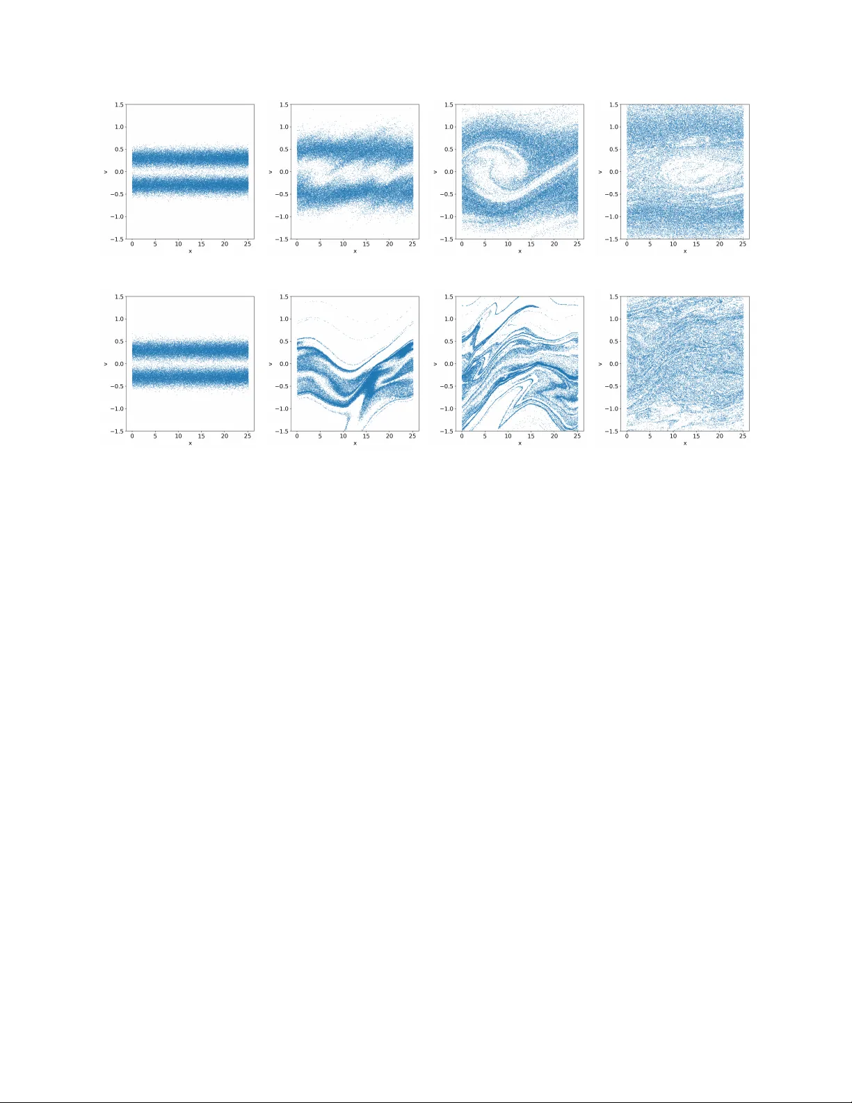
DEEP KINETIC JK O SCHEMES F OR VLASO V-F OKKER-PLANCK EQUA TIONS W ONJUN LEE, LI W ANG, AND WUCHEN LI Abstract. W e in tro duce a deep neural netw ork–based n umerical method for solving kinetic F okker Planc k equations, including both linear and nonlinear cases. Building upon the conserv ativ e dissi- pativ e structure of Vlaso v-t ype equations, we form ulate a class of generalized minimizing mo v emen t sc hemes as iterative constrained minimization problems: the conserv ative part determines the con- strain t set, while the dissipativ e part defines the ob jectiv e functional. This leads to an analog of the classical Jordan–Kinderlehrer–Otto (JKO) scheme for W asserstein gradient flows, and we refer to it as the kinetic JK O scheme. T o compute each step of the kinetic JKO iteration, w e introduce a particle-based approximation in which the velocity field is parameterized by deep neural net works. The resulting algorithm can be interpreted as a kinetic-orien ted neural differential equation that enables the representation of high-dimensional kinetic dynamics while preserving the essential v ari- ational and structural properties of the underlying PDE. W e v alidate the method with extensive n umerical exp erimen ts and demonstrate that the prop osed kinetic JK O–neural ODE framework is effectiv e for high-dimensional numerical simulations. 1. Introduction Man y dynamical mo dels in complex systems from ph ysics, c hemistry , and engineering exhibit a conserv ativ e–dissipative structure [2, 10, 27]: part of the evolution is reversible and preserv es an energy-lik e quan tit y , while the remaining part is irreversible and driv es the system tow ard equilibrium through entrop y dissipation. Examples range from kinetic equations with collisions to viscous and diffusive contin uum mo dels to thermo dynamic systems. In this pap er, w e fo cus on designing numerical schemes for a particular class of conserv a- tiv e–dissipativ e systems, namely the kinetic F okk er–Planck equation, which pla ys a cen tral role in plasma physics and dynamical densit y functional theory [33]. A represen tativ e form is: ∂ t f + v · ∇ x f − ∇ x ϕ · ∇ v f = ∇ v · ( v f + ∇ v f ) , (1) where f is a probability densit y function defined on the phase space ( x , v ) ∈ Ω x × R d . ϕ ( x ) ∈ R 1 represen ts an external p oten tial function, which may either be prescrib ed a priori or determined self-consisten tly . The left-hand side of (1) describ es the reversible Hamiltonian dynamics, under whic h the Hamiltonian functional H [ f ] = Z 1 2 | v | 2 f + ϕ ( x ) f d x d v , is conserved. In contrast, the righ t-hand side represents the dissipativ e dynamics, which drives the system to ward lo cal equilibrium b y dissipating a relative en trop y functional S [ f ] = Z 1 2 | v | 2 f + f log f d x d v . There is also a free energy E [ f ], defined as the sum of H and the negativ e Shannon–Boltzmann en trop y R f log f , d x , d v , which dissipates along the dynamics (1). Key wor ds and phr ases. Kinetic JKO sc hemes; Neural ODEs; Vlaso v-F okker-Planc k Equations, Symplectic inte- grator; Conserv ative-dissipativ e structure. 1 DEEP KINETIC JKO SCHEMES 2 Sim ulating system (1) remains a challenging task. One central difficult y , as emphasized in [27], is the preserv ation of the underlying conserv ative-dissipativ e structure under suitable time- and spatial-discretization sc hemes, which is essential for ensuring reliability and ph ysical fidelit y in n umerical simulations. Another obstacle arises from the high dimensionalit y of the mo dels, which are p osed in a sev en-dimensional phase space: 3 in x , 3 in v , and 1 in t . As a result, grid-based metho ds rapidly b ecome computationally infeasible due to the curse of dimensionality . Instead, mac hine learning based approaches, suc h as neural ODEs [8, 11, 29], ha v e emerged as promising alternativ es for approximating high-dimensional probabilit y densities. In particular, for equations that con tain only the dissipativ e part and does not depend on the spatial v ariable, that is, ∂ t f ( t, v ) = ∇ v · ( v f ( t, v ) + ∇ v f ( t, v )) or more generally ∂ t f ( t, v ) = ∇ v · ( f u [ f ]) , (2) where u [ f ] ∈ R d is a velocity field that may dep end linearly or nonlinearly on f , sev eral learning- enhanced metho ds hav e been dev elop ed to address the c hallenge of high dimensionality [4, 26, 22, 13, 25, 18, 16, 15, 35]. Among these, transp ort-based approac hes ha v e attracted noticeable attention [4, 22]. The k ey idea starts from the particle representation of (2). Specifically , let { v i ( t ) } N i =1 b e a set of i.i.d. samples drawn from f ( t, · ). Their ev olution is then gov erned b y d d t v i ( t ) = u ( f ( v 1 , · · · , v N )) . (3) The task is to infer the velocity field u directly from the particle ensemble, without explicitly accessing the density f . Approac hes such as score matc hing [4] and v elocity matc hing [22] hav e b een dev elop ed to accomplish this goal. Another approac h also relies on the particle representation (3). How ever, instead of up dating the particles explicitly , it learns the v elocity field implicitly through the minimizing mo v emen t scheme, also known as the JKO scheme [20]. More precisely , one views (2) as the W asserstein gradient flow ∂ t f ( t, v ) = ∇ v · ( f ∇ v δ S δ f ) , where δ δ f is the L 2 first v ariation op erator w.r.t. function f , and with a sligh t abuse of notation, S is the relativ e entrop y for f only in v ariable v . Given a time approximation function f n ( · ) ≈ f ( t n , · ), the JK O scheme determines f n +1 ( · ) ≈ f ( t n +1 , · ) with t n +1 = ( n + 1)∆ t through: f n +1 ∈ arg min f n W 2 2 ( f , f n ) + 2∆ t S ( f ) o . (4) Here, W 2 ( f , f n ) denotes the W asserstein-2 distance betw een f and f n . The scheme in (4) can b e in terpreted as a time-implicit scheme of gradient descent, where the functional on the right-hand side acts as the W asserstein proximal operator asso ciated with S . Using the dynamic form ulation of the W asserstein distance [1], (4) can b e reformulated as [5]      ( f , u ) = arg inf f , u Z 1 0 Z R d f | u | 2 d v d τ + 2∆ t S ( f (1 , · )) , s.t. ∂ τ f + ∇ v · ( f u ) = 0 , f (0 , v ) = f n ( v ) . (5) Let d d τ T ( τ , v ) = v ( τ , T ( τ , v )) , T (0 , v ) = v . DEEP KINETIC JKO SCHEMES 3 denote the flow map asso ciated with the velocity field u . Using a particle approximation of the densit y , (5) can b e translated in to the following optimization problem o v er the velocity field:          min u 1 N N X j =1  Z 1 0 | u ( τ , T ( τ , v j )) | 2 d τ + 2∆ tV ( T (1 , v j ))  + 2∆ t S ( T # f n ) , s.t. d d τ T ( τ , v j ) = u ( τ , T ( τ , v j )) , T (0 , v j ) = v n j . (6) F urther details can b e found in [21]. When considering the full system (1), an additional requiremen t is the conserv ation of the Hamil- tonian. While general metho ds suc h as velocity matc hing [22, 36] can b e applied directly to (1) in the extended phase space ( x , v ), the resulting mo dels do not necessarily preserv e the desired conserv ative–dissipativ e structure. In this work, we instead exploit the intrinsic decomp osition of kinetic equations in to conserv ativ e Hamiltonian and dissipativ e gradien t flo w comp onents. Our main idea is to introduce a v ariant of the formulation (5), in which the conserv ative dynamics are enco ded in the constraint set, while the dissipative dynamics determine the ob jective functional. W e refer to this v ariational formulation as the kinetic JKO scheme . In this wa y , b oth the conserv a- tiv e and dissipativ e structures of the system are naturally preserv ed. Moreo v er, the JK O framew ork guaran tees the monotonic decay of the associated Ly apuno v functional, such as the free energy . W e note that generalized JK O sc hemes for kinetic equations hav e b een studied in [14, 10], particu- larly within the framework of general Equation for Non-equilibrium reversible–irrev ersible coupling (GENERIC) [27] and macroscopic fluctuation theory (MFT) [3]. Ho w ev er, that w ork primarily fo cuses on the theoretical properties, suc h as Kan toro vich formulations, of v ariational problems and does not aim to pro vide efficient and scalable n umerical algorithms. In contrast, our approac h mak es this feasible b y com bining a particle representation with a densit y ev olution parameterized through a neural ODE. Another related line of work is based on the idea of score-matc hing. F or instance, [25, 4, 18, 16] apply score matc hing methods to appro ximate mean-field F okk er-Planck equations. Some asp ects of conv ex analysis for the score-based matching optimization metho d for t w o-lay er neural netw ork functions ha v e been studied [34]. Additionally , [13, 19, 23, 24, 37] hav e studied neural pro jected sc hemes, whic h can be view ed as semi-time-discretizations of the neural net w ork-based computational method. Compared with the ab o v e-mentioned existing works, our approac h is v ariational: time discretization is p erformed at the level of a constrained minimiza- tion problem. This structure provides enhanced numerical stability and ensures compatibilit y with energy dissipation. The rest of the pap er is organized as follows. Section 2 reviews the kinetic F okker–Planc k equation and its conserv ative–dissipativ e decomposition from a free energy dissipation persp ective. W e illustrate this decomp osition for both linear and nonlinear cases. Section 3 introduces the generalized kinetic JK O sc heme in Eulerian co ordinates and then studies its implemen tation in Lagrangian co ordinates. W e employ kinetic neural ODEs to approximate the logarithm of the densit y and discuss the numerical properties of the resulting metho d, including the free energy dissipation. Section 4 presen ts n umerical exp erimen ts that v erify the sc heme’s accuracy , stability , and scalabilit y . The paper concludes in Section 5. 2. Kinetic F okker-Planck equa tion In this section, w e review the kinetic F okker–Planc k equation, in b oth its linear and nonlinear forms, and highlight its conserv ative–dissipativ e structure. 2.1. Linear case. Consider the Vlasov-F okker-Planc k equation ∂ t f + v · ∇ x f − ∇ x ϕ · ∇ v f = ϵ ∇ v · ( v f + ∇ v f ) , (7) DEEP KINETIC JKO SCHEMES 4 where f := f ( t, x , v ) denotes the phase-space num ber densit y of charged particles at time t , lo cation x and with velocity v . The function ϕ ( x ) is a given p oten tial, with x ∈ R d or a compact subset Ω x ⊂ R d , and v ∈ R d . Unless stated otherwise, when Ω x is compact, w e imp ose p erio dic boundary conditions in the spatial v ariable x . And ϵ > 0 mo dels the strength of the collision. W e b egin b y rewriting (7) in a form that clearly reveals its conserv ative–dissipativ e structure. Sp ecifically , it can b e written as: ∂ t f = ∇ x , v ·  f J ∇ x , v δ E δ f  | {z } conserv ativ e + ∇ x , v ·  f D ∇ x , v δ E δ f  | {z } dissipative , (8) where the free energy is defined as E [ f ] := Z R d Z Ω x | v | 2 2 f + ϕ ( x ) f + f log f d x d v . (9) Here J ∈ R 2 d × 2 d is an an ti-symmetric matrix and D ∈ R 2 d × 2 d is a symmetric positive semi-definite matrix D =  0 0 0 ϵ I  , J =  0 − I I 0  . And I is an iden tit y matrix in R d × d , and the op erator δ δ f is the L 2 first v ariation w.r.t. function f . Indeed, the form (8) follows from a direct computation. Note that δ E [ f ] δ f = | v | 2 2 + ϕ ( x ) + log f + 1 , and ∇ x , v δ E [ f ] δ f =  ∇ x ϕ ( x ) + ∇ x log f v + ∇ v log f  . Clearly , ∇ x , v ·  f J ∇ x , v δ E δ f  = ∇ x , v ·  f  − v − ∇ v log f ∇ x ϕ ( x ) + ∇ x log f  = ∇ x , v ·  f  − v ∇ x ϕ ( x )  , where in the last equality , w e use the fact that f ∇ x , v log f = ∇ x , v f , and ∇ x , v ·  f  −∇ v log f ∇ x log f  = ∇ x , v ·  −∇ v f ∇ x f  = 0 . Similarly , we ha v e ∇ x , v ·  f D ∇ x , v δ E δ f  = ∇ x , v ·  f  0 v + ∇ v log f  = ∇ v ·  f v + ∇ v f  , where w e use the fact that f ∇ v log f = ∇ v f . Since D + J is non-degenerate, it follows from (8) that the equilibrium o ccurs when ∇ x,v δ δ f E [ f ] = 0, whic h implies that δ δ f E [ f ] = Constant. Therefore, the in v ariant distribution of equation (7) satisfies f ∞ ( x , v ) = 1 Z e − ( | v | 2 2 + ϕ ( x )) , where Z is a normalization constant satisfying Z = Z R d Z Ω x e − ( | v | 2 2 + ϕ ( x )) d x d v < + ∞ . DEEP KINETIC JKO SCHEMES 5 The follo wing free energy dissipation result holds. Prop osition 1. Supp ose f ( t, · ) is the solution of e quation (7) . Then d dt E [ f ]( t, · ) = − Z R d Z Ω x ( ∇ x , v δ δ f E [ f ] , D ∇ x , v δ δ f E [ f ]) f d x d v ≤ 0 , (10) wher e E [ f ] is define d in (9) . Pr o of. The pro of is b y a direct computation, with an emphasis on the semi-p ositive definite matrix D and the symplectic matrix J . d dt E [ f ] = Z R d Z Ω x ∂ t f · δ δ f E d x d v = Z R d Z Ω x  ∇ x , v ·  f J ∇ x , v δ E δ f  + ∇ x , v ·  f D ∇ x , v δ E δ f   · δ δ f E d x d v = − Z R d Z Ω x  ( ∇ x , v δ δ f E , J ∇ x , v δ δ f E ) + ( ∇ x , v δ δ f E , D ∇ x , v δ δ f E )  f d x d v = − Z R d Z Ω x ( ∇ x , v δ δ f E , D ∇ x , v δ δ f E ) f d x d v ≤ 0 , where we use the fact that J is a symplectic matrix suc h that u T J u = 0, for any vector u ∈ R 2 d . This finishes the pro of. □ W e note that equation (8) is not a gradien t flo w due to the presence of the anti-symmetric matrix J . Nev ertheless, in the follo wing sections, we will in troduce a v ariational formulation of (8) that main tains the asso ciated free energy dissipation prop erty (10). 2.2. Nonlinear case. Consider the Vlasov-P oisson-F okker-Planc k system:    ∂ t f + v · ∇ x f − ∇ x ϕ · ∇ v f = ϵ ∇ v · ( v f + T 0 ∇ v f ) , x ∈ Ω ⊂ R d x , − ∆ x ϕ = ρ ( t, x ) − h , ρ ( t, x ) = Z R d f d v . (11) This equation is commonly used to model a single-sp ecies plasma, describing the motion of electrons in a static ion background, where h is a constant representing the bac kground charge. It satisfies the global neutrality condition Z Ω x h d x = Z Ω x ρ ( t, x )d x . Here, T 0 is a given background temp erature (consider the ion as a steady thermal bath). Compared to (7), the main difference here is that ϕ is not giv en apriori, but obtained self- consisten tly through the P oisson equation. In theory , one can obtain it using the Green’s function G , suc h that ϕ ( x ) = Z Ω x G ( x − y )( ρ ( t, y ) − h )d y . (12) Similar to Prop osition 1, this nonlinear system (11) also satisfies free energy dissipation. Prop osition 2. F or e quation (11) , define the Lyapunov functional: E [ f ] := Z R d Z Ω x  1 2 | v | 2 f + T 0 f log f  d x d v + 1 2 Z Ω x |∇ x ϕ | 2 d x . Then d d t E [ f ]( t ) ≤ 0 . DEEP KINETIC JKO SCHEMES 6 Pr o of. Note first that 1 2 Z Ω x |∇ x ϕ | 2 d x = − 1 2 Z Ω x ϕ ∆ x ϕ d x = 1 2 Z Ω x ϕ ( ρ − h )d x = 1 2 Z Ω x Z Ω x ( ρ ( t, x ) − h ) G ( x − y )( ρ ( t, y ) − h )d x d y . Then (11) can also b e written in the form of (8), with δ δ f  1 2 Z Ω x ∥∇ x ϕ ∥ 2 d x  = G ∗ ( ρ − h ) = ϕ ( x ) . The rest pro of follow the same argumen t as in Prop osition 1. □ W e note a closely related v ariant of (11), the Vlasov–Ampere–F okker–Planc k system, which is giv en by    ∂ t f + v · ∇ x f + E · ∇ v f = ϵ ∇ v · ( v f + T 0 ∇ v f ) , ∂ t E ( t, x ) = − J ( t, x ) , J ( t, x ) = Z R d v f d v . (13) One can readily show that if the initial electric field E (0 , x ) satisfies ∇ x · E (0 , x ) = ρ (0 , x ) − h , then, since E ev olv es according to (13), this relation is preserv ed for all time: ∇ x · E ( t, x ) = ρ ( t, x ) − h . Indeed, in tegrating the f equation in (13) with respect to v yields the contin uit y equation ∂ t ρ = −∇ x · J . T aking the divergence of the evolution equation for E then gives ∂ t ∇ x · E = ∂ t ρ . Since ∇ x · E and ρ − h satisfy the same ev olution equation and agree initially , they coincide for all t ≥ 0. If we write E = −∇ x ϕ , then we recov er the Poisson equation. Consequen tly , it also satisfies the same free energy dissipation prop erty . In fact, the Vlasov–Amp ` ere–F okker–Planc k system also enjo ys the follo wing dissipation property for a general initial condition E (0 , x ). Prop osition 3. F or e quation (13) , define the ener gy functional E [ f ] := Z R d Z Ω x  1 2 | v | 2 f + T 0 f log f  d x d v + 1 2 Z Ω x | E ( t, x ) | 2 d x , then d d t E [ f ] = − ϵ Z R d Z Ω x ∥ T 0 ∇ v log f e − ∥ v ∥ 2 2 T 0 ∥ 2 f d x d v ≤ 0 . Pr o of. Let ( f , E ) b e the solution to (13). Then we can rewrite it as: ∂ t f = ϵT 0 ∇ v · f ∇ v log f e − | v | 2 2 T 0 ! − ∇ x , v ·  f  v E ( t, x )  , DEEP KINETIC JKO SCHEMES 7 where w e used f ∇ v log f = ∇ v f . Then we ha v e d dt E [ f ] = Z R d Z Ω x ( T 0 log f + T 0 + 1 2 | v | 2 ) · ∂ t f d x d v + Z Ω x E · ∂ t E d x = − ϵ Z R d Z Ω x ∥ T 0 ∇ v log f e − | v | 2 2 T 0 ∥ 2 f d x d v + Z R d Z Ω x  T 0 ∇ x log f · v + T 0 ∇ v log f · E + v · E  f d x d v − Z Z E · v f d x d v = − ϵ Z R d Z Ω x ∥ T 0 ∇ v log f e − | v | 2 2 T 0 ∥ 2 f d x d v . In the last equality of the abov e form ula, w e use the fact that Z R d Z Ω x  T 0 ∇ x log f · v + T 0 ∇ v log f · E  f d x d v = Z R d Z Ω x  T 0 ∇ x f · v + T 0 ∇ v f · E  d x d v = − Z R d Z Ω x  T 0 f ∇ x · v + T 0 f ∇ v · E  d x d v = 0 . This finishes the pro of. □ 3. Generalized JK O formula tion and p ar ticle method In this section, we prop ose the generalized JKO form ulation for kinetic F okker-Planc k equations. W e then apply a v ariational particle metho d in which the v elo cit y is constructed using the neural ODE metho d. 3.1. Generalized JKO form ulation. W e prop ose the follo wing generalized dynamical JKO for- m ulation of (7) or (8). Given f n ( x , v ) at time t = t n := n ∆ t , w e obtain f n +1 ( x , v ) as follows:              min f , u 1 2∆ t Z 1 0 Z R d Z Ω x ( | u | 2 f )( τ , x , v )d x d v d τ + ϵ E [ f (1 , · , · )] , E [ f ] := Z R d Z Ω x [ | v | 2 2 + ϕ ( x )] f + f log f d x d v , s.t. ∂ τ f + ∆ t v · ∇ x f − ∆ t ∇ x ϕ · ∇ v f + ∇ v · ( u f ) = 0 , f (0 , x , v ) = f n ( x , v ) . (14) Compared to the v anilla dynamical JKO for W asserstein gradien t flo w (5), the main difference lies in the additional term ∆ t ( v · ∇ x f − ∇ x ϕ · ∇ v f ) in the constrain t PDE. This term arises from the conserv ative part of the PDE, specifically the term inv olving J in (8). This is in tuitiv e b ecause the conserv ative part is what prev en ts the original equation from b eing a gradien t flow. W e also note that if we only consider the dissipative term in (8), the asso ciated energy should b e R R d R Ω x | v | 2 2 f + f log f d x d v . Ho w ev er, it is imp ortant to retain the full energy in the formulation. Including the full energy do es not alter the optimalit y condition, but it is crucial for ensuring that the algorithm preserves the energy dissipation prop ert y stated in the following proposition. Prop osition 4 (F ree energy dissipation for (14)) . L et f n +1 ( x , v ) b e the solution to (14) , then we have E [ f n +1 ] ≤ E [ f n ] , wher e E is define d in (9) . Pr o of. Note first that E [ f n +1 ] ≤ E [ ˜ f ] , where ˜ f is obtained by solving ∂ τ ˜ f + ∆ t v · ∇ x ˜ f − ∆ t ∇ x ϕ · ∇ v ˜ f = 0 , ˜ f (0 , x , v ) = f n ( x , v ) . DEEP KINETIC JKO SCHEMES 8 No w w e claim that E [ ˜ f ] = E [ f n ]. T o establish this, we need to sho w that the energy E [ f ] is conserv ed along the flow: ∂ t f + v · ∇ x f − ∇ x ϕ · ∇ v f = 0 . (15) Let H [ f ] := Z R d Z Ω x [ | v | 2 2 + ϕ ( x )] f d x d v , H 0 [ f ] = Z R d Z Ω x f log f d x d v , then E [ f ] = H [ f ] + H 0 [ f ]. First, it is direct to chec k that d d t H [ f ] = 0 for f satisfying (15). T o c hec k H 0 [ f ], w e see that d H 0 d t = Z δ H 0 δ f ∇ x , v ·  f J ∇ x , v δ E δ f  d x d v = Z δ E δ f ∇ x , v ·  f J ∇ x , v δ H 0 δ f  d x d v = Z δ E δ f ∇ x , v · ( J ∇ x , v f ) d x d v = 0 , where the last equalit y is due to f ∇ x , v log f = ∇ x , v f and the anti-symmetry prop erty of matrix J . □ No w we translate (14) using the flow mapping function. Denote T ( τ , x n , v n ) = ( x ( τ ; x n ) , v ( τ ; v n )) ⊤ , where x ( τ , x n ), v ( τ ; x n ) are solutions to the following ODE system d d τ x ( τ ) = ∆ t v ( τ ) , x (0) = x 0 , d d τ v ( τ ) = − ∆ t ∇ x ϕ ( x ( τ )) + u ( τ , x ( τ ) , v ( τ )) , v (0) = v 0 . W e state the follo wing prop osition, whic h we term kinetic neural ODEs. It ma y b e regarded as a generalization of the neural ODE framework dev elop ed in [21]. Prop osition 5 (Kinetic neural ODEs) . The fol lowing e quation holds: d d τ log | det ∇ x , v T ( τ , x , v ) | = ∇ v ( τ ) · u ( τ , T ( τ , x , v )) . (16) Pr o of. Equation (16) is derived from the Monge-Ampere equation. Assume that T ( τ , x , v ) is in- v ertible, i.e. | det ∇ x , v T ( τ , x , v ) |  = 0. Denote ξ ( x ( τ ) , v ( τ )) := d d τ T ( τ , x , v ) = ( v ( τ )∆ t, −∇ x ϕ ( x ( τ ))∆ t + u ( τ , x ( τ ) , v ( τ ))) . Then d d τ log det |∇ x , v T ( τ , x , v ) | =tr  ( ∇ x , v T ( τ , x , v )) − 1 d d τ ∇ x , v T ( τ , x , v )  =tr  ( ∇ x , v T ( τ , x , v )) − 1 ∇ x , v d d τ T ( τ , x , v )  =tr  ( ∇ x , v T ( τ , x , v )) − 1 ∇ x , v ξ ( x ( τ ) , v ( τ ))  = ∇ x ( τ ) , v ( τ ) · ξ ( T ( τ , x , v )) = ∇ v ( τ ) · u ( τ , T ( τ , x , v )) , where the first equality uses the Jacobi identit y , and the second last equalit y uses the c hain rule. □ DEEP KINETIC JKO SCHEMES 9 W e appro ximate u b y u θ with θ ∈ Θ b eing the parameters. W e assume that the family { u θ } θ ∈ Θ is sufficiently expressiv e to approximate a broad class of vector fields on R d × R d . Since the inner time is discretized using a single time step, we employ a fully connected neural netw ork that takes ( x , v ) ∈ R d × R d as input and outputs a vector in R d . A typical arc hitecture has the form u θ ( t, x , v ) = W L σ ( W L − 1 σ ( · · · σ ( W 1 ( x , v ) + b 1 ) · · · ) + b L − 1 ) + b L , where L denotes the n um ber of la y ers, W k and b k are trainable weigh t matrices and bias vectors, and σ ( z ) = max( αz , z ) is the LeakyReLU activ ation function with slope parameter α > 0. Let m 0 = 2 d + 1 denote the input dimension, corresponding to the concatenated v ariable ( x , v ). Let m 1 , . . . , m L − 1 denote the hidden lay er widths and m L = d the output dimension. Then the net w ork parameters satisfy W k ∈ R m k × m k − 1 , b k ∈ R m k , k = 1 , . . . , L . The parameter vector θ consists of all trainable w eigh ts and biases, θ = { W 1 , b 1 , . . . , W L , b L } , whic h may b e iden tified with a v ector in R d θ , where d θ = P L k =1 ( m k m k − 1 + m k ) denotes the total n um b er of parameters in the netw ork. Then (14) rewrites as:                                            min θ 1 2∆ t Z 1 0 Z R d Z Ω x | u θ ( τ , x ( τ ; x n ) , v ( τ ; v n )) | 2 f n ( x n , v n )d x n d v n d τ + Z R d Z Ω x [ | v | 2 2 + ϕ ( x ) + log f ](1 , x (1; x n , v n ) , v (1; x n , v n )) f n ( x n , v n )d x n d v n , s.t. d d τ x ( τ ) = ∆ t v ( τ ) , x (0) = x n , d d τ v ( τ ) = − ∆ t ∇ x ϕ ( x ( τ )) + u θ ( τ , x ( τ ) , v ( τ )) , v (0) = v n , d d τ log | det ∇ x , v T ( τ ) | = ∇ v · u θ ( τ , x ( τ ) , v ( τ )) , log | det ∇ x , v T (0) | = 0 , f ( τ , x ( τ ) , v ( τ )) = f n ( x n , v n ) | det ∇ x , v T ( τ ) | . (17) 3.2. P article method. W e no w discretize (17) using particles in space and symplectic in tegrator in time. Given i.i.d. N samples { ( x n p , v n p ) } N p p =1 ∼ f n ( x , v ), w e solv e the follo wing optimization problem:                              min θ ∆ t 2 1 N p N p X p =1 | u θ ( x n p , v n p ) | 2 + ϵ N p N p X p =1  1 2 | v n +1 p | 2 + ϕ ( x n +1 p ) + log f n +1 ( x n +1 p , v n +1 p )  , s.t. x n +1 p = x n p + v n +1 p ∆ t , v n +1 p = v n p − ∇ x ϕ ( x n p )∆ t + u θ ( x n p , v n p )∆ t , log | det ∇ x , v T ( x n +1 p , v n +1 p ) | = ∇ v · u θ ( x n p , v n p )∆ t , f n +1 ( x n +1 p , v n +1 p ) = f n ( x n p , v n p ) | det ∇ x , v T ( x n +1 p , v n +1 p ) | . (18) It is worth noting that the up date in the constraint can be replaced b y a more general form:  x n +1 p v n +1 p  = S ( x n p , v n p ) +  0 u θ ( x n p , v n p )∆ t  , (19) DEEP KINETIC JKO SCHEMES 10 where S : ( x n p , v n p ) 7→ ( x ∗ p , v ∗ p ) , (20) is an explicit symplectic mapping. This generalization do es not violate the up date formula for the log determinan t or the density that appeared in the third and fourth equations in the constrain t ab o v e. Belo w w e list tw o simple choices for S . F or a more comprehensiv e discussion of symplectic in tegrators, we refer to [12]: 1) Sympletic Euler metho d: ( x ∗ p = x n p + v n p ∆ t , v ∗ p = v n p − ∇ x ϕ ( x ∗ p )∆ t ; (21) 2) Stormer–V erlet metho d:            v n +1 / 2 p = v n p − ∆ t 2 ∇ x ϕ ( x n p ) , x ∗ p = x n p + ∆ t v n +1 / 2 p , v ∗ p = v n +1 / 2 p − ∆ t 2 ∇ x ϕ ( x ∗ p ) . (22) W e v erify the optimality condition for (18) to ensure that the constrained optimization problem indeed yields the correct optimizer u θ . Denote J [ u θ ] := 1 N p N p X p =1  ∆ t 2 | u θ ( x n p , v n p ) | 2 + ϵ 2 | v n +1 p | 2 + ϵϕ ( x n +1 p ) + ϵ log f n +1 ( x n +1 p , v n +1 p )  . (23) By substituting the constraint in to the ob jective function in (23), w e hav e ∂ ∂ u θ ( x n p , v n p ) J = 1 N p  ∆ t u θ ( x n p , v n p ) + ϵ v n +1 p ∆ t + ϵ ∇ x ϕ ( x n +1 p )∆ t 2 + ϵ ∇ x log f n +1 ( x n +1 p , v n +1 p )∆ t 2 + ϵ ∇ v log f n +1 ( x n +1 p , v n +1 p )∆ t  . Setting ∂ ∂ u θ J = 0, we ha v e u θ ( x n p , v n p ) = − ϵ v n +1 p − ϵ ∇ v log f n +1 ( x n +1 p , v n +1 p ) + O (∆ t ) , (24) whic h is consistent with the expected drift form from the dissipative part of (7). W e also note that Prop osition 4 can b e extended to the Lagrangian formulation. In particular, w e hav e the follo wing prop osition. Prop osition 6. L et x ( τ ; x n ) and v ( τ ; v n ) b e the solution to (17) , define E ( τ ) = Z R d Z Ω x  1 2 | v ( τ ; v n ) | 2 + ϕ ( x ( τ ; x n )) + log f ( x ( τ ; x n ) , v ( τ ; v n ))  f n ( x n , v n )d x n d v n . Then we have E (1) ≤ E (0) . Pr o of. Starting from (17), we first observe that E (1) ≤ ˜ E (1), where ˜ E is obtained by setting u θ to zero. More precisely , define ˜ E ( τ ) = Z R d Z Ω x  1 2 | ˜ v ( τ ; v n ) | 2 + ϕ ( ˜ x ( τ ; x n )) + log f ( ˜ x ( τ ; x n ) , ˜ v ( τ ; v n ))  f n ( x n , v n )d x n d v n , DEEP KINETIC JKO SCHEMES 11 where            d d τ ˜ x ( τ ) = ∆ t ˜ v ( τ ) , ˜ x (0) = x n , d d τ ˜ v ( τ ) = − ∆ t ∇ x ϕ ( ˜ x ( τ )) , ˜ v (0) = v n , d d τ log | det ∇ x , v T ( τ ) | = 0 , log | det ∇ x , v T (0) | = 0 , f ( τ , ˜ x ( τ ) , ˜ v ( τ )) = f n ( x n , v n ) | det ∇ x , v T ( τ ) | . (25) It is obvious that Z R d Z Ω x [ 1 2 | ˜ v ( τ ) | 2 + ϕ ( ˜ x ( τ ))] f n ( x n , v n )d x n d v n , is preserv ed along the dynamics. W e also claim that Z log f ( ˜ x ( τ ) , ˜ v ( τ )) f n ( x n , v n )d x n d v n , is not changing, and this is guaranteed b y the fact that | det ∇ x , v T ( τ ) | ≡ 1 along the dynamics (25). Then the result concludes b ecause ˜ E (1) = ˜ E (0) = E (0). □ Remark 1. We emphasize that fr e e ener gy dissip ation at the semi-discr ete level do es not auto- matic al ly c arry over to the ful ly discr ete scheme, sinc e the symple ctic up date (20) is not exactly ener gy-c onserving. Nevertheless, the symple ctic discr etization pr eserves ener gy up to a smal l err or and exhibits stable long-time b ehavior. Algorithm 1 Deep Kinetic JKO sc heme based on (18) Require: T erminal time T > 0, time step ∆ t > 0, num b er of particles N p , collision strength ϵ > 0, initial particles { ( x 0 p , v 0 p , f 0 ) } N p p =1 , n um ber of inner optimization steps K , a parametrized function u θ with parameters θ . Ensure: Appro ximate particle state at time T . 1: Set M = ⌈ T / ∆ t ⌉ . 2: for n = 0 , 1 , . . . , M − 1 do 3: Compute the p oten tial ϕ n and the gradient vector field −∇ x ϕ n from { x n p } N p p =1 . 4: Initialize net work parameters θ ← θ (0) . 5: for k = 1 , . . . , K do 6: P erform one optimization step to approximately solv e (18) and up date θ . 7: end for 8: for p = 1 , . . . , N do 9: Up date v elo cit y: v n +1 p = v n p − ∇ x ϕ n ( x n p )∆ t + u θ ( x n p , v n p )∆ t. 10: Up date p osition: x n +1 p = x n p + v n +1 p ∆ t. 11: Up date densit y: f n +1 ( x n +1 p , v n +1 p ) = f n ( x n p , v n p )   det ∇ x , v T ( x n +1 p , v n +1 p )   . 12: end for 13: end for 14: return { ( x M p , v M p , f M ) } N p p =1 . DEEP KINETIC JKO SCHEMES 12 Remark 2. In pr actic e, the Jac obian determinant app e aring in (18) is appr oximate d thr ough the diver genc e of the neur al c ontr ol field, log | det ∇ x , v T ( x , v ) | ≈ ∆ t ∇ v · u θ ( x , v ) , as sp e cifie d by the c onstr aint in (18) . The diver genc e ∇ v · u θ is evaluate d by automatic differ entiation within the neur al network fr amework. Mor e pr e cisely, e ach p artial derivative ∂ u θ,i /∂ v i is c ompute d by b ackpr op agation, and the diver genc e is obtaine d by summation over the velo city c omp onents. This appr o ach avoids the explicit c onstruction of the ful l Jac obian matrix and enables an efficient and sc alable evaluation of the entr opy pr o duction term for lar ge p article ensembles and high-dimensional velo city sp ac es. 3.3. Discussion on other form ulations. 3.3.1. Op er ator splitting. It is w orth noting that (18) with the up date (21) or (22) is equiv alent to an alternativ e op erator-splitting discretization. In particular, the problem can b e splitted into the follo wing substeps: Step 1: Vlasov comp onen t:     x ∗ p v ∗ p  = S ( x n p , v n p ) , f ∗ ( x ∗ p , v ∗ p ) = f n ( x n p , v n p ) . (26) Step 2: F okker-Planc k comp onen t:                              min θ ∆ t 2 1 N N X p =1 | u θ ( x ∗ p , v n p ) | 2 + ϵ N N X p =1 1 2 | v n +1 p | 2 + log f n +1 ( x ∗ p , v n +1 p ) , s.t. x n +1 p = x ∗ p , v n +1 p = v ∗ p + u θ ( x ∗ p , v n p )∆ t , log | det ∇ x , v T ( x ∗ p , v n +1 p ) | = ∇ v · u θ ( x ∗ p , v n p )∆ t , f n +1 ( x n +1 p , v n +1 p ) = f ∗ ( x ∗ p , v ∗ p ) | det ∇ x , v T ( x ∗ p , v n +1 p ) | . (27) While the split form ulation ma y appear straightforw ard, w e note that the non-split form ulation has its o wn merits, as it pro vides a natural extension from gradien t flo ws to non-gradient-flo w systems and ma y offer new insights in to the analytical structure and stability properties of the equation. 3.3.2. V elo city matching. If one views (7) as a generic transp ort equation in the com bined phase space ( x , v ), then the v elocity matching approach of [22, 30] applies naturally . More precisely , one seeks to match the v elo cit y field u with A ∇ x , v δ E δ f b y solving the following v ariational problem:      ( f , u ) = arg min f , u Z T 0 Z Ω x , v f | u + A ∇ x , v δ E δ f | 2 d x d v d t , s.t. ∂ t f + ∇ x , v · ( f u ) = 0 , f (0 , x , v ) = f 0 ( x , v ) , (28) where A = D + J . W e parameterize the v elocity field as u ( t, x , v ) = u θ ( t, x , v ) and denote by f θ the corresp onding densit y induced by the contin uit y equation. F ollowing the fixed-p oin t iteration strategy in [22], problem (28) can b e solved iterativ ely via      θ k +1 ∈ arg min θ Z T 0 Z Ω x , v f θ k | u θ + A ∇ x , v δ E δ f θ k | 2 d x d v d t , s.t. ∂ t f θ k + ∇ x , v · ( f θ k u θ k ) = 0 , f (0 , x , v ) = f 0 ( x , v ) . (29) DEEP KINETIC JKO SCHEMES 13 Substituting the explicit form of E from (9) in to (29), the ob jective function can b e simplified as follo ws (for notational conv enience, w e omit the subscript θ k in f ): F := Z T 0 Z Ω x , v [ | u x θ − ( v + ∇ v log f ) | 2 + | u v θ + ( ∇ x ϕ + ∇ x log f ) − ( v + ∇ v log f ) | 2 ] f d x d v d t = Z T 0 Z Ω x , v [ | u x θ | 2 − 2 u x θ · v + | u v θ | 2 + 2 u v θ · ∇ x ϕ − 2 u v θ · v + 2 ∇ v · u x θ − 2 ∇ x · u v θ + 2 ∇ v · u v θ )] f d x d v d t + constant , (30) where u = ( u x , u v ). The integral (30) can be ev aluated directly using samples from f , thereby completely a v oiding explicit densit y estimation. This simplification is enabled b y the score matching principle [17]. Compared to our form ulation (14), the form ulation (28) differs in t w o main asp ects. (i) It adopts an end-to-end training strategy , rather than the sequential training used in (14). This approac h has b oth adv antages and dra wbac ks: on the one hand, it a v oids repeated retraining ov er time b y learning a time-dep endent velocity field in a single stage; on the other hand, the resulting training problem can b e significan tly more c hallenging. (ii) It do es not explicitly preserve the conserv ative–dissipativ e structure of the equation; consequen tly , these structural prop erties are not inheren tly enforced in the formulation. 3.3.3. Sc or e b ase d tr ansp ort mo deling. Another approac h that has been studied extensiv ely is score- based transp ort modeling, which can be viewed as a simplified v arian t of (28). Instead of learning the entire velocity field, this metho d fo cuses on le arning only the comp onent that cannot b e rep- resen ted directly by particles, namely the score function. This idea was first introduced in [4] and subsequen tly extended to the mean-field F okker–Planc k equation in [25], as well as to the Landau equation in [16, 18]. In particular, when considering the end-to-end setting, one arrives at the follo wing formulation, which parallels (28):      ( f , u ) = arg min f , u Z T 0 Z Ω x , v f | u − ∇ v log f | 2 d x d v d t , s.t. ∂ t f + v · ∇ x f − ∇ x ϕ · ∇ v f − ∇ v · ( v f ) − ∇ v · ( u f ) = 0 , f (0 , x , v ) = f 0 ( x , v ) . (31) Comparing (31) with (28), the ob jective function in (31) in v olv es few er terms and is therefore easier to optimize. It is w orth noting that score-based dynamics w ere in tro duced by [31], from the self- consistency of the F okker-Planc k equation. The numerical approximation of score dynamics is an indep enden t c hallenge in its own righ t. F or example, [22] prop oses an iterative metho d with a biased gradien t estimator to a v oid the estimation of the score function directly . In contrast, our metho d em b eds both the conserv ativ e Hamiltonian and the dissipativ e gradien t-flo w mechanisms directly within a constrained v ariational framework. This form ulation extends the structure-preserving prop erties of deep JK O schemes from W asserstein gradien t flo ws to kinetic equations. A brief n umerical comparison will b e presented in Section 4.1. 3.4. Extension to the nonlinear system. W e extend the generalized dynamical JK O sc heme (18) to the nonlinear setting. T o handle the P oisson equation, we employ a particle-in-cell method [32, 7]. Here, the subscript p denotes particles, while the subscript h denotes grid p oints. In particular, ( x n p , v n p ) represent the p osition and v elo cit y of particle p at time t n , and x h denotes the DEEP KINETIC JKO SCHEMES 14 h -th grid p oin t, which remains fixed in time. The sc heme takes the follo wing form:                            min θ ∆ t 2 1 N N X p =1 | u θ ( x n p , v n p ) | 2 + ϵ N N X p =1  1 2 | v n +1 p | 2 + T 0 log f n +1 ( x n +1 p , v n +1 p )  + X h | E n +1 h | 2 (∆ x ) d , s.t. x n +1 p = x n p + v n p ∆ t , v n +1 p = v n p + E n +1 p ∆ t + u θ ( x n p , v n p )∆ t , log | det ∇ x , v T ( x n +1 p , v n +1 p ) | = ∇ v · u θ ( x n p , v n p )∆ t , f n +1 ( x n +1 p , v n +1 p ) = f n ( x n , v n ) | det ∇ x , v T ( x n +1 p , v n +1 p ) | . (32) where the field term E is computed as follows: E n +1 p = X h S ( x n +1 p − x h ) E n +1 h , E n +1 h = −∇ x ϕ n +1 h , − ∆ x ϕ n +1 h = ρ n +1 h − 1 , ρ n +1 h = 1 ∆ x X p ω p S ( x h − x n +1 p ) , ω p = 1 N . Here, the index h represen ts the index of a p oin t x h whic h is a cen ter p oin t of eac h grid cell, S ( x ) is a lo cal basis function, such that 1 | cell h | R cell h S ( x )d x = 1. A common c hoice is the tent function S ( z ) = max { 0 , 1 − | z | ∆ x } . Remark 3. We note that her e we employ an explicit symple ctic inte gr ator for the Hamiltonian p art, which is not exactly ener gy-c onserving. Nevertheless, one c an fol low the nic e appr o ach pr op ose d in [28] to enfor c e exact ener gy c onservation. This adaptation is str aightforwar d in our setting, and we ther efor e do not pursue it further her e. 4. Numerical examples In this section, w e present numerical results to demonstrate the effectiv eness of our proposed metho d. W e first consider several linear kinetic F okk er-Planc k equations with kno wn analytical solutions to v alidate the accuracy of our approach. W e then apply our method to nonlinear kinetic F okker-Planc k equations, particularly the Vlaso v-P oisson-F okker-Planc k system, demonstrating its capabilit y to handle complex interactions and long-time b eha viors. 4.1. Linear kinetic F okker-Planc k equations. Here w e present t w o examples of linear kinetic F okker-Planc k equations: one with an explicit solution o v er time, and another with an explicit solution only at equilibrium. Both serve as initial testbeds for our prop osed metho d. W e present results in b oth 1D p osition–1D velocity and 3D position–3D velocity settings. Example 1: Gaussian cases with explicit solutions W e b egin with a simple test case where the solution to the kinetic F okker-Planc k equation remains Gaussian o v er time. Sp ecifically , w e consider the state v ariable x = ( x, v ), where x, v ∈ R d . Assume there exists a positive definite matrix K ∈ R 2 d × 2 d and a vector ˜ µ ∈ R 2 d suc h that the potential function ϕ ( x ) satisfies v 2 2 + ϕ ( x ) = 1 2 ( x − ˜ µ ) ⊤ K − 1 ( x − ˜ µ ) . Supp ose the initial distribution is f (0 , x ) ∼ N ( µ 0 , C 0 ). Then the solution to the kinetic equation (7) remains Gaussian: f ( t, x ) ∼ N ( µ ( t ) , C ( t )) , DEEP KINETIC JKO SCHEMES 15 Algorithm 2 Kinetic JKO sc heme based on (32) Require: T erminal time T > 0, time step ∆ t > 0, num b er of particles N , collision strength ϵ > 0, initial particles { ( x 0 p , v 0 p , f 0 ) } N p =1 , n um ber of inner optimization steps K , a parametrized function u θ with parameters θ . Ensure: Appro ximate particle state at time T . 1: Set M = ⌈ T / ∆ t ⌉ . 2: for n = 0 , 1 , . . . , M − 1 do 3: P osition update: 4: for p = 1 , . . . , N do 5: x n +1 p = x n p + v n p ∆ t ; 6: end for 7: Field update: 8: Compute grid density ρ n +1 h = 1 ∆ x P p 1 N S ( x h − x n +1 p ) from new p ositions. 9: Solv e the discrete Poisson equation − ∆ x ϕ n +1 h = ρ n +1 h − 1. 10: Compute E n +1 h = −∇ x ϕ n +1 h and in terp olate to particles: E n +1 p = P h S ( x n +1 p − x h ) E n +1 h . 11: Neural net w ork optimization: 12: Initialize net work parameters θ ← θ (0) . 13: for k = 1 , . . . , K do 14: P erform one optimization step to minimize the loss in (32) and up date θ . 15: end for 16: V elo cit y and density up date: 17: for p = 1 , . . . , N do 18: x n +1 p = x n p + v n p ∆ t ; 19: v n +1 p = v n p + E n +1 p ∆ t + u θ ( x n p , v n p )∆ t ; 20: f n +1 ( x n +1 p , v n +1 p ) = f n ( x n p , v n p ) exp  −∇ v · u θ ( x n p , v n p )∆ t  ; 21: end for 22: end for 23: return { ( x M p , v M p , f M ) } N p =1 . where µ ( t ) and C ( t ) evolv e according to ˙ µ ( t ) = − ( D + J ) K − 1 ( µ ( t ) − ˜ µ ) , (33a) ˙ C ( t ) = 2 D − 2 Sym  ( D + J ) K − 1 C ( t )  , (33b) with initial conditions µ (0) = µ 0 , C (0) = C 0 , and Sym( A ) = 1 2 ( A + A ⊤ ) . In the 1D case ( d = 1), w e choose K =  1 2 0 0 1  , ˜ µ =  0 0  , whic h corresp onds to the p otential ϕ ( x ) = x 2 . The initial condition is set as µ 0 = (0 , 1) ⊤ and C 0 =  2 1 1 3  . W e then simulate the dynamics of (7). Since the exact solution remains Gaussian, the optimal con trol field can b e w ell appro ximated b y an affine function. T o exploit this structure, w e parameterize the neural netw ork mo del for u θ ( x, v ) DEEP KINETIC JKO SCHEMES 16 as a single-lay er affine map: u θ ( x, v ) = W θ  x v  + b θ , where W θ ∈ R d × 2 d and b θ ∈ R d . This parameterization is sufficien t to capture the true con trol dynamics in this setting while keeping the model simple and efficient to train. The con trol field u θ is trained using the prop osed v ariational form ulation giv en in (18) and Algorithm 1. T o assess the accuracy of this approach, we compare it against a score-matching metho d, whic h directly estimates the score function ∇ v log f from samples. T o establish a ground truth for this comparison, we compute the exact solution by solving the ODE system (33) for the mean and cov ariance of the Gaussian distribution, yielding f exact . W e then ev aluate the drift error at each time step n , defined as the squared difference betw een the learned field u θ and the exact analytical field: Error 2 ( n ) = 1 N p N p X p =1   u n θ ( x n p , v n p ) + v n +1 p + ∇ v log f n +1 exact ( x n +1 p , v n +1 p )   2 . (34) Figure 1 demonstrates the temp oral conv ergence of the proposed method detailed in Algorithm 1. It plots the time-a v eraged drift error, computed from t = 0 to the terminal time T = 8, as a function of the time step size ∆ t . F or b oth the 1D and 3D sim ulations, we use N p = 10 , 000 particles, where ( x n p , v n p ) denotes the state of the p -th particle at time step n . The reference exact densit y , f exact , is generated using a highly refined time step of ∆ t ref = 10 − 4 to ensure high accuracy . As indicated b y the dashed reference lines, the prop osed metho d exhibits a linear, first-order ( O (∆ t )) con vergence rate. Figure 2 compares the p erformance of our prop osed method against the score-matc hing approac h o v er time. The left panel trac ks the drift error (computed via (34)) at each individual time step to highligh t the relativ e accuracy of the t w o methods. The righ t panel illustrates the energy decay exclusiv ely for our prop osed algorithm. The discrete energy at time step n is calculated as: Energy( n ) = 1 N p N p X p =1  1 2 | v n +1 p | 2 + ϕ ( x n +1 p ) + log f n +1 ( x n +1 p , v n +1 p )  . (35) These experiments w ere conducted ov er the time in terv al [0 , 10] for the 1D case and [0 , 20] for the 3D case, both utilizing a discrete time step of ∆ t = 0 . 1. F or the neural net w ork architectures, b oth configurations used fully connected net w orks with Tanh activ ations b etw een lay ers. Sp ecifically , the 1D mo del consisted of 2 hidden la y ers with 16 units each, while the 3D mo del used 2 hidden la y ers with 32 units each. In the 1D case, our algorithm exhibits stable and consisten tly low error throughout the time in terv al, whereas the score-matching metho d sho ws noticeable oscillations, suggesting some insta- bilit y in the drift appro ximation. In the 3D case, the score-based mo del p erforms well during the early phase, yielding smaller errors up to t ≈ 6, but its accuracy appears to plateau thereafter. In contrast, our algorithm con tin ues to impro v e ov er time and even tually attains lo w er errors for t > 6. Example 2. Conv ergence to the stationary distribution In the second exp eriment, w e in v estigate the conv ergence of the learned solution to w ard the stationary equilibrium. W e first consider 1 D in x and 1 D in v case ∂ t f + v ∂ x f − ∂ x ϕ ∂ v f = ∂ v ·  v f + ∂ v f  , (36) DEEP KINETIC JKO SCHEMES 17 (a) 1D (b) 3D Figure 1. Drift error vs. time step size ∆ t for Example 1 in the 1D (left) and 3D (righ t) cases. The plots demonstrate linear con v ergence b ehavior as the time step decreases. The dashed lines indicate a reference O (∆ t ) con v ergence rate. with initial condition ρ 0 ( x ) = N (0 , 1) , f 0 ( x, v ) = ρ 0 ( x ) 2 √ 2 π  exp  − | v +1 . 5 | 2 2  + exp  − | v − 1 . 5 | 2 2  , and the p oten tial function ϕ ( x ) = 1 2 x 2 + cos(2 π x ) . The stationary distribution corresp onding to (36) is known explicitly as f ∞ ( x, v ) = C exp  − v 2 2 − ϕ ( x )  , (37) where C is the normalization constant ensuring R f ∞ ( x, v )d x d v = 1. As sho wn in [9], solutions to (36) con verge exp onentially fast to (37) in relative en trop y . T o appro ximate this b eha vior numerically , we represen t the velocity field u θ with a neural netw ork consisting of t w o hidden la y ers with 16 neurons and Tanh activ ation. The time step is c hosen to be ∆ t = 0 . 1, adv anced up to final time T = 10, yielding 100 outer iterations. Figure 3 visualizes the evolution of the densit y pro duced by the algorithm from t = 0 to t = 2. The plots show conv ergence tow ard the expected stationary solution: the stationary distribution is dra wn as con tours, while the computed solution app ears as a densit y map in whic h ligh ter regions indicate higher particle density . The close o v erlap b etw een high-densit y regions and the con tours demonstrates accurate conv ergence. Figure 4 presen ts tw o complementary diagnostics. Panel (A) displays the x - and v -marginals of the computed solution at t = 10 together with the stationary marginals. The close o v erlap indicates that the numerical metho d attains high accuracy at late times. Pan el (B) rep orts the Kullbac k–Leibler divergence b et w een the computed distribution and the stationary distribution for t ∈ [0 , 10] under the particle JKO dynamics, where an exp onen tial decay is observ ed. Example 3. p erio dic domain In the third exp eriment, similar to the second experiment, w e in v estigate the con v ergence of the learned solution tow ard the stationary equilibrium of a kinetic F okker–Planc k–t ype equation but the only c hange is the b oundary condition. Here, we consider DEEP KINETIC JKO SCHEMES 18 (a) 1D: error plot (b) 1D: energy plot (c) 3D: error plot (d) 3D: energy plot Figure 2. Drift error plots using (24) compare the errors b et w een our algorithm and the score-based model for Example 1 in the 1D case (left) and the 3D case (righ t). The 1D exp eriment was conducted o v er the time in terv al from 0 to 10 with a time step of 0.1, while the 3D exp eriment w as run from 0 to 20 with the same time step. The same parameters, including the neural netw ork arc hitecture, were used for b oth exp erimen ts and b oth metho ds. the p erio dic boundary condition on x space, follo wing the setup in [6]. W e consider the same one- dimensional-in-space and one-dimensional-in-velocity kinetic equation in (36) posed on x ∈ [0 , 1] with p erio dic b oundary conditions and v ∈ R . The initial condition is chosen as the pro duct of a p erio dic function in x and a symmetric mixture of Gaussians in v : ρ 0 ( x ) = 1 + 1 2 cos(2 π x ) , f 0 ( x, v ) = ρ 0 ( x ) 2 √ 2 π  exp  − | v +1 . 5 | 2 2  + exp  − | v − 1 . 5 | 2 2  . W e test the following external p oten tial: ϕ s ( x ) = 1 5 sin(2 π x ) . (38) W e appro ximate the v elo cit y field u θ using a neural net w ork with t w o hidden lay ers of 16 neurons eac h. T o accommodate p erio dic boundary conditions in this exp erimen t, we enforce p erio dicit y directly in the neural net work inputs. Specifically , for a given state ( x, v ), the netw ork takes (sin(2 π x ) , cos(2 π x ) , v ) as its input. The evolution of the particle system is adv anced iterativ ely using the proposed algorithm in Algorithm 1. F or eac h discrete time step n , the algorithm computes the state transition to the subsequent step n + 1 using a fixed step size of ∆ t = 0 . 1. This pro cess DEEP KINETIC JKO SCHEMES 19 (a) t = 0 . 00 (b) t = 1 . 00 (c) t = 10 . 00 Figure 3. Evolution of the distribution from t = 0 to t = 2 from Exp erimen t 2 with step size 0 . 1. The results sho w con v ergence tow ard the stationary distribution at t = 2. Bright regions indicate areas of high particle densit y , darker regions indicate lo w density , and the con tours represent the stationary solution. (a) Sine potential (b) KL div ergence ov er time Figure 4. (A) The x -marginal and v -marginal at time t = 10. (B) Con v ergence of the Kullback–Leibler divergence to the stationary distribution for t ∈ [0 , 10] under the particle JKO dynamics from Exp erimen t 2. is rep eated up to a final time of T = 20, yielding 200 outer iterations. The densit y ev olution for b oth c hoices of the potential function is rep orted in Figure 5. In b oth cases, the learned solution con v erges to the stationary state, confirming the exp ected long-time b eha vior. Figure 6 summarizes the b eha vior of the numerical solution through three plots. The first t wo panels compare the empirical marginals with their stationary targets, namely f x t v ersus π x ( x ) ∝ e − ϕ ( x ) and f v t v ersus N (0 , 1). The ov erla ys show strong agreement in b oth x -marginal and v - marginal. The third panel shows the con vergence of the Kullback–Leibler divergence b et w een the computed solution and the exact stationary distribution ov er the time interv al t ∈ [0 , 20]. At eac h time step, the n umerical solution is represented b y an ensem ble of particles { ( x n p , v n p ) } N p p =1 . The stationary distribution f ∞ is kno wn in closed form from (37). The Kullbac k–Leibler div ergence D KL  f n ∥ f ∞  = Z f n ( x , v ) log  f n ( x , v ) f ∞ ( x , v )  d x d v , is therefore approximated using a Monte Carlo estimator based on the particle ensem ble. Sp ecifi- cally , w e ev aluate the Kullbac k-Leibler (KL) div ergence using a Monte Carlo approximation ov er DEEP KINETIC JKO SCHEMES 20 the particle ensemble: D KL  f n ∥ f ∞  ≈ 1 N p N p X p =1  log f n ( x n p , v n p ) − log f ∞ ( x n p , v n p )  . In the implemen tation, the exact log-densit y log f n ( x n p , v n p ) is ev aluated b y dynamically trac king it for eac h particle along its tra jectory . Starting from the analytically kno wn initial distribution, the log-density is up dated at eac h discrete time step using the linearized log-determinant of the pushforw ard mapping (i.e., log f n +1 = log f n − ∆ t ∂ v u θ ). F or the stationary distribution, the analytical formula from (37) is used. The resulting KL div ergence curv es decrease substan tially o v er time, demonstrating rapid con v ergence of the numerical solution to the stationary distribution. (a) t = 0 . 00 (b) t = 0 . 50 (c) t = 1 . 00 (d) t = 1 . 50 (e) t = 2 . 00 Figure 5. Experiment from Example 3. Evolution of the distribution from t = 0 to t = 2 with step size 0 . 1, using the sine p otential. The results show con v ergence to w ard the stationary distribution at t = 2. Brigh t regions indicate areas of high particle densit y , darker regions indicate low density , and the con tours represen t the stationary solution. (a) Sine potential (b) KL from a sine potential Figure 6. Experiment from Example 3. The x - and v -marginal densities at t = 20 under the p oten tial defined in (38). The righ t plot sho ws the con v ergence of the Kullbac k–Leibler divergence to the stationary distribution ov er the time interv al t ∈ [0 , 20] for the particle JKO dynamics under t w o external p otentials. Example 4: Conv ergence to the stationary distribution in 3D. W e extend Example 2, which w as posed in one spatial dimension and one velocity dimension, to the three–dimensional setting in b oth x and v to demonstrate that the algorithm computes an accurate solution that conv erges to w ard the exp ected stationary distribution. F or this 3D exp eriment, the external p oten tial is ϕ ( x ) = 1 2 ∥ x ∥ 2 2 + 3 X i =1 cos(2 π x i ) , DEEP KINETIC JKO SCHEMES 21 whic h com bines a quadratic confining term with small co ordinate–wise p erio dic bumps. The asso- ciated stationary density f ∞ on R 3 × R 3 is f ∞ ( x, v ) ∝ exp  − 1 2 ∥ v ∥ 2 2 − ϕ ( x )  , so the v –marginal is N (0 , I 3 ) and eac h co ordinate x i has a one–dimensional stationary density prop ortional to exp( − 1 2 x 2 i − cos(2 π x i )). W e initialize particles from f 0 ( x, v ) = 1 2(2 π ) 3  e − ( v 1 +1 . 5) 2 2 + e − ( v 1 − 1 . 5) 2 2  e − v 2 2 + v 2 3 2 e − ∥ x ∥ 2 2 . T o illustrate the distribution of particles ov er time, w e pro ject the data on to one-dimensional marginals for b oth the spatial and v elo cit y coordinates. W e then construct empirical histograms using 160 bins for b oth the x and v marginals to approximate the underlying densities. These are o v erlaid with the analytical stationary distributions to facilitate visual comparison. Across runs, w e observ e a monotone decrease of D KL ( f t ∥ f ∞ ) together with increasing alignment of eac h marginal with its stationary coun terpart, indicating conv ergence tow ard f ∞ . This b ehavior is illustrated in Figures 7 and 8. Figure 8 further quantifies this trend for Exp erimen t 4 o v er the time window t ∈ [0 , 5] with time step ∆ t = 0 . 1. W e rep ort the evolution of the KL divergence, whic h exhibits a steady monotone deca y , alongside the corresp onding marginal discrepancies. Consistently decreasing trends are ob- serv ed across all coordinates, indicating that b oth spatial and v elocity components relax tow ard equilibrium. The agreement b etw een empirical marginals and their stationary targets at selected times pro vides additional evidence supp orting conv ergence of the full distribution tow ard f ∞ . 4.2. Vlaso v–P oisson–F okk er–Planc k systems (PIC–JKO metho d). W e study a 1D in space and 1D in v elo cit y Vlaso v–P oisson–F okker–Planc k (VPFP) system on a p eriodic domain. The dynamics are computed using a particle-in-cell (PIC) discretization for the kinetic density and a sp ectral Poisson solver for the self-consisten t electric field. The evolution follows the pro ximal form ulation describ ed in Section 3.4, where each JK O step is implemen ted through a neural control field that is trained at every time step. The spatial domain is x ∈ [0 , 8 π ) with perio dic b oundary conditions, discretized b y N x = 128 grid points with spacing ∆ x = 8 π / N x . Cell cen ters are giv en b y x i = ( i + 1 2 )∆ x for i = 0 , . . . , N x − 1. The v elo cit y v ariable v ∈ R remains unbounded in the dynamics. A time step of ∆ t = 10 − 2 is used, and the simulation adv ances for n steps = 200 iterations, yielding a final time T = 4. The distribution function f ( t, x, v ) is represented b y N p = 50 , 000 equal-weigh t particles ( x p , v p , ω ). The initial spatial density is ρ 0 ( x ) = 1 8 π (1 + α cos( k x )) , α = 0 . 1 , k = 0 . 2 , and the initial phase-space distribution is f 0 ( x, v ) = ρ 0 ( x ) 2 √ 2 π 0 . 1  e − ( v − 0 . 3) 2 2(0 . 1) 2 + e − ( v +0 . 3) 2 2(0 . 1) 2  , where the marginal in v is a symmetric mixture of Gaussians centered at ± 0 . 3 with standard deviation 0 . 1 (v ariance 0 . 01). T o sample particles from the nonuniform spatial profile ρ 0 ( x ), w e use inv erse transform sampling. The density is first ev aluated on the discrete grid { x i } and normalized to form a probabilit y mass function p i = ρ 0 ( x i ) / P j ρ 0 ( x j ). The corresponding cum ulativ e distribution function P i = P j ≤ i p j maps uniform random v ariables u ∼ Uniform(0 , 1) to grid indices i satisfying P i − 1 < u ≤ P i , thereb y pro ducing samples consistent with ρ 0 ( x ). Each c hosen grid p oin t x i is then p erturb ed by a small random displacement within [ − 1 2 ∆ x, 1 2 ∆ x ] to remo v e grid bias. The v elo cit y samples are dra wn indep enden tly from a normal distribution v p ∼ N (0 , T 0 ) with T 0 = 1. DEEP KINETIC JKO SCHEMES 22 (a) t = 0 (b) t = 0 . 5 (c) t = 1 Figure 7. Evolution of co ordinate marginals for a 3D position v ariable x = ( x 1 , x 2 , x 3 ) with 3D velocity v , computed with time step ∆ t = 0 . 1. Eac h panel sho ws the one–dimensional marginals of x 1 , x 2 , and x 3 at the indicated time: (a) t = 0, (b) t = 0 . 5, (c) t = 1. Eac h particle contributes to the grid densit y through a piecewise-linear basis function S ( x ) = max  0 , 1 − | x | / ∆ x  , whic h spreads the particle w eigh t o ver neigh b oring grid p oin ts. The grid densit y at cell h is computed as ρ h = 1 ∆ x N X p =1 1 N S ( x h − x p ) . A t every time step, w e solve the perio dic Poisson equation − ∂ xx ϕ = ρ − 1 , E = − ∂ x ϕ , DEEP KINETIC JKO SCHEMES 23 (a) KL div ergence ov er time x marginals (b) KL div ergence ov er time v marginals Figure 8. Con v ergence of the Kullbac k–Leibler div ergence, x marginals, and v marginals to the stationary distribution for t ∈ [0 , 5] under the particle JKO dy- namics, sho wn for Exp eriment 4. using a sp ectral method. The discrete F ourier frequencies are k j = 2 π fftfreq( N x , ∆ x ) , and the solution is obtained as b ϕ ( k ) = \ ( ρ − 1)( k ) k 2 ( k  = 0) , b ϕ (0) = 0 , b E ( k ) = − i k b ϕ ( k ) , follo w ed b y an inv erse transform to reco v er ϕ and E in ph ysical space. The electric field is then in terp olated to particle lo cations using the same linear basis function to ensure consistency b et w een dep osition and in terp olation. Let t n = n ∆ t . One JKO update adv ances particles according to x n +1 p = wrap x ( x n p + v n p ∆ t ) , v n +1 p = v n p + E n +1 ( x n +1 p )∆ t + u θ ( x n p , v n p )∆ t , where wrap x ( x ) = ( x mo d 8 π ) enforces p erio dicit y . The control field u θ : R 2 → R is a feedforward neural netw ork with inputs (cos( x/ 2) , sin( x/ 2) , v ), t w o hidden lay ers of width 32 with LeakyReLU activ ations, and a linear output lay er. The mapping T ( x, v ) = ( x + v ∆ t, v + E n +1 ( x + v ∆ t )∆ t + u θ ( x, v )∆ t ) defines the discrete transport, and its Jacobian determinan t is computed using auto- matic differen tiation. A t each time step and for a fixed parameter ϵ > 0, the net work parameters θ are optimized by minimizing J ( θ ) = ∆ t 2 N p X p =1 [ u θ ( x n p , v n p ) 2 ] + ϵ N p X p =1  1 2 ( v n +1 p ) 2 + T 0 log f n +1 p  + X i ( E n +1 i ) 2 ∆ x , where the exp ectations are empirical av erages ov er the particles. Each minimization uses 50 Adam iterations with a learning rate of 10 − 3 , after whic h the optimized con trol is applied to adv ance the system. The field energy E field ( t ) = P i E 2 i ∆ x is recorded at every step, and a phase-space histogram H i,j estimating f ( t, x i , v j ) is sav ed every ten steps. Two parameter regimes are studied, ϵ ∈ { 10 , 10 − 2 } , with all other settings fixed: N x = 128 , N p = 50 , 000 , ∆ t = 10 − 2 , n steps = 200 , N opt = 50 , lr = 10 − 3 . F or the weakly collisional case ϵ = 5 × 10 − 3 , the field energy R | E | 2 d x exhibits mild oscillations paired with a slow o v erall decay (Figure 9, left). The initial transient sho ws a rapid drop follow ed b y a substantial p eak near t ≈ 0 . 8, driven b y the stretching of the particle distribution and w eak damping. After t ≈ 1, the energy fluctuates p ersistently b et w een 10 − 3 and 10 − 2 . F or the strongly collisional case ϵ = 10, the field energy exhibits a highly noisy but rapid ov erall decay (Figure 9, DEEP KINETIC JKO SCHEMES 24 righ t), dropping b elow 10 − 3 b y t ≈ 2 and approac hing 10 − 4 b y t = 4. While the deca y is not strictly steady due to high-frequency fluctuations, the clear down w ard tra jectory demonstrates that the larger regularization parameter enhances velocity diffusion. Figure 10 further illustrates these contrasting b eha viors by tracking the discrete particle p ositions in phase space at distinct time snapshots. F or the w eakly collisional case with ϵ = 0 . 005 (top row), the initial v elo cit y bands roll up to form a large, coheren t phase-space v ortex by t = 0 . 6. This large-scale structure, c haracterized by a distinct cen tral empty region, persists ev en at the final time t = 4 . 0. This persistence sho ws that the particles are trapped and maintain their organized motion due to the w eak damping. Conv ersely , for the strongly collisional case with ϵ = 10 (b ottom ro w), the initial bands undergo severe stretching and folding b y t = 0 . 6, thereb y b ypassing the formation of a stable v ortex. By t = 4 . 0, the particles ha v e scattered significan tly and filled the phase-space regions that remained empty in the low- ϵ scenario. These scatter plots highlight ho w a stronger collision dictates the behavior by breaking do wn organized particle structures and rapidly driving the discrete system tow ard a w ell-mixed equilibrium. (a) ϵ = 5 × 10 − 3 (b) ϵ = 10 Figure 9. Exp eriment from Section 4.2.Comparison of field energy deca y R | E | 2 dx o v er time for ϵ = 5 × 10 − 3 (left) and ϵ = 10 (righ t). Extended exp eriment: 1 D in space and 3 D in v elo cit y . T o assess the p erformance of the prop osed JK O-based scheme in higher-dimensional phase space, w e extend the one-dimensional v elo cit y experiment to a setting with one spatial v ariable and three velocity comp onen ts, x ∈ [0 , 8 π ) and v = ( v 1 , v 2 , v 3 ) ∈ R 3 . The spatial domain is p erio dic, and the electric field is determined by the one-dimensional P oisson equation in x , so that the field acts only on the first velocity comp onent v 1 . The initial distribution is chosen as f 0 ( x, v ) = ρ 0 ( x ) 2(2 π σ 2 ) 3 / 2  e − ( v 1 − 1 . 5) 2 2 σ 2 + e − ( v 1 +1 . 5) 2 2 σ 2  e − v 2 2 + v 2 3 2 σ 2 , σ = 0 . 1 . (39) The spatial marginal is prescrib ed by ρ 0 ( x ) = 1 8 π  1 + 0 . 005 cos(2 π x )  , so that R R 3 f 0 ( x, v ) d v = ρ 0 ( x ). This configuration represen ts t w o coun ter-propagating b eams in the v 1 direction with small ther- mal spread, combined with isotropic Gaussian fluctuations in the transverse v elo cit y comp onents DEEP KINETIC JKO SCHEMES 25 (a) t = 0 . 0 (b) t = 0 . 2 (c) t = 0 . 6 (d) t = 4 . 0 (e) t = 0 . 0 (f) t = 0 . 2 (g) t = 0 . 6 (h) t = 4 . 0 Figure 10. Exp eriment from Section 4.2. Phase-space densit y f ( t, x, v ) for ϵ = 0 . 005 (top row) and ϵ = 10 (b ottom row) at differen t times. v 2 and v 3 . Compared with the 1 D x–1 D v exp eriment, the phase space dimension increases from t w o to four, providing a non trivial test of the scalability of the method. Initial particle p ositions are sampled according to the discrete appro ximation of ρ 0 ( x ) on the spatial grid, follow ed by uniform jitter within each cell. V elo cities are dra wn from the mixture distribution in (39). The initial particle w eigh ts are assigned according to f 0 ( x, v ), ensuring con- sistency with the prescrib ed density . The neural control field u θ ( x, v ) ∈ R 3 is appro ximated by a fully connected feedforward neural net w ork. T o respect the p erio dicity in the spatial v ariable, the input la y er consists of the fiv e features  cos( x/ 4) , sin( x/ 4) , v 1 , v 2 , v 3  , whic h pro vides a smo oth embedding of the spatial co ordinate and the three velocity comp onen ts. The netw ork contains tw o hidden la y ers with 64 neurons eac h and LeakyReLU activ ation functions, follo w ed b y a linear output la y er pro ducing a three-dimensional v ector corresp onding to the v elocity comp onen ts of the control field. All remaining parameters, including the time step, grid resolution, and optimization settings, are iden tical to those used in the 1D–1D exp eriment, except that the terminal time is set to T = 4 instead of T = 4 in this exp erimen t. In particular, we consider both weak and strong regularization regimes to facilitate direct comparison. This extended exp eriment demonstrates that the proposed algorithm remains stable and accurate in higher-dimensional velocity spaces, while preserving the qualitative kinetic structures observed in low er dimensions. In particular, the w eakly regularized case exhibits sustained oscillations, while the strongly regularized case displa ys rapid monotone deca y , consistent with the b ehavior observ ed in the 1D–1D exp eriment. As in the one-dimensional velocity setting, a coheren t vortex structure also emerges in the weakly regularized regime, indicating the onset of nonlinear trapping and b eam–b eam in teraction. DEEP KINETIC JKO SCHEMES 26 Figure 11 illustrates the ev olution of the phase-space density pro jected on to the ( x, v 1 ) plane for b oth ϵ = 0 . 005 and ϵ = 10. F or ϵ = 0 . 005, fine filamentary structures, beam in teractions, and the formation of a rotating v ortex p ersist o v er time, whereas for ϵ = 10 the distribution rapidly smo oths and b ecomes unimo dal. T ogether, these results confirm that the prop osed metho d successfully captures filamentation, beam in teraction, v ortex formation, and long-time relaxation in the presence of transverse velocity fluctuations, illustrating its robustness and scalabilit y with increasing dimension. (a) t = 0 . 0 (b) t = 0 . 4 (c) t = 1 . 2 (d) t = 4 . 0 (e) t = 0 . 0 (f) t = 0 . 4 (g) t = 1 . 2 (h) t = 4 . 0 Figure 11. Experiment from Section 4.2. Phase-space density f ( t, x, v 1 ) pro jected on to the ( x, v 1 ) plane for the 1 D –3 D setting, with ϵ = 0 . 005 (top ro w) and ϵ = 10 (b ottom ro w) at different times. 5. Conclusions JK O schemes provide a v ariational framework for approximating nonlinear gradient flo ws. In this paper, we extend the classical JKO framew ork to kinetic equations through a conserv a- tiv e–dissipativ e decomposition. The resulting kinetic JK O sc heme is implemen ted using particle ap- pro ximations together with kinetic-orien ted neural ODEs. This approach preserves the v ariational structure of kinetic equations and ensures dissipation of a modified energy functional. Numerical exp erimen ts on high-dimensional linear and nonlinear Vlasov–F okk er–Planck systems demonstrate the accuracy and effectiveness of the proposed metho d. F uture researc h directions include dev eloping deep neural net w ork–based solvers for more general kinetic equations that exhibit a conserv ativ e–dissipativ e structure. Another imp ortan t direction is to conduct a detailed numerical analysis of kinetic JK O schemes with neural ODE appro xima- tions. Sev eral la yers of error analysis w arran t careful in v estigation, including appro ximation error, optimization error, and sample complexity . It will also b e v aluable to systematically compare the prop osed metho d with score matc hing and velocity field matching metho ds, particularly with resp ect to their numerical stability and long-time b eha vior. DEEP KINETIC JKO SCHEMES 27 Ac kno wledgmen t: W. Li is supp orted b y the AFOSR YIP a w ard No. F A9550-23-1-0087, NSF R TG: 2038080, NSF FRG: 2245097, and the McCausland F aculty F ello wship at the Universit y of South Carolina. L. W ang is partially supp orted by NSF grants DMS-2513336 and Simons F ellow- ship. L. W ang also thanks Profs. Phillip Morrison and Luk as Eink emmer for fruitful discussions. W. Lee ackno wledges funding from the National Institute of Standards and T ec hnology under a w ard n um b er 70NANB22H021 and startup funding from The Ohio State Universit y . References [1] J. Benamou and Y. Brenier , A c omputational fluid me chanics solution to the Monge-Kantor ovich mass tr ans- fer pr oblem , Numer. Math., 84 (2000), pp. 375–393. [2] L. Ber tini, A. De Sole, D. Gabrielli, G. Jona-Lasinio, and C. Landim , Macr osc opic fluctuation the ory , Rev. Mo d. Phys., 87 (2015), pp. 593–636. [3] , Macrosc opic fluctuation the ory , Rev. Mo d. Phys., 87 (2015), pp. 593–636. [4] N. M. Boffi and E. V anden-Eijnden , Pr obability flow solution of the F okker–Planck e quation , Machine Learn- ing: Science and T echnology , 4 (2023), p. 035012. [5] J. A. Carrillo, K. Craig, L. W ang, and C. Wei , Primal dual metho ds for Wasserstein gr adient flows , F ound. Comput. Math., 22 (2022), pp. 389–443. [6] J. A. Carrillo, L. W ang, W. Xu, and M. Y an , V ariational asymptotic pr eserving scheme for the Vlasov– Poisson–F okker–Planck System , Multiscale Mo deling & Simulation, 19 (2021), pp. 478–505. [7] G. Chen, L. Cha c ´ on, and D. C. Barnes , An ener gy-and char ge-c onserving, implicit, ele ctr ostatic p article-in- c el l algorithm , Journal of Computational Physics, 230 (2011), pp. 7018–7036. [8] R. T. Q. Chen, Y. Rubano v a, J. Bettencour t, and D. Duvenaud , Neur al or dinary differ ential e quations , in Adv ances in Neural Information Pro cessing Systems (NeurIPS), 2018. [9] L. Desvillettes and C. Villani , On the tr end to glob al e quilibrium in sp atial ly inhomo gene ous entr opy- dissip ating systems: The line ar F okker-Planck e quation , Communications on Pure and Applied Mathematics: A Journal Issued by the Courant Institute of Mathematical Sciences, 54 (2001), pp. 1–42. [10] M. H. Duong, M. A. Peletier, and J. Zimmer , Conservative–dissip ative appr oximation schemes for a gen- er alize d Kr amers e quation , Mathematical Methods in the Applied Sciences, (2014). [11] E. Haber and L. R uthotto , Stable ar chite ctur es for de ep neur al networks , Inv erse Problems, 34 (2018), p. 014004. [12] E. Hairer, M. Hochbruck, A. Iserles, and C. Lubich , Ge ometric numeric al inte gr ation , Ob erwolfac h Rep orts, 3 (2006), pp. 805–882. [13] Z. Hu, C. Liu, Y. W ang, and Z. Xu , Ener getic variational neur al network discr etizations of gr adient flows , SIAM Journal on Scientific Computing, 46 (2024), pp. A2528–A2556. [14] C. Huang , A variational principle for the kr amers e quation with unbounde d external for c es , Journal of Mathe- matical Analysis and Applications, 250 (2000), pp. 333–367. [15] Y. Huang and L. W ang , JKO for landau: a variational p article metho d for homo gene ous landau e quation , arXiv preprint arXiv:2409.12296, (2024). [16] , A sc or e-b ase d p article metho d for homo gene ous L andau e quation , Journal of Computational Physics, (2025), p. 114053. [17] A. Hyv ¨ arinen and P. D a y an , Estimation of non-normalize d statistic al mo dels by sc or e matching. , Journal of Mac hine Learning Research, 6 (2005). [18] V. Ilin, J. Hu, and Z. W ang , T r ansp ort b ase d p article metho ds for the F okker-Planck-L andau e quation , Com- m unications in Mathematical Sciences, 23 (2025), pp. 1763–1788. [19] Y. Jin, S. Liu, H. Wu, X. Ye, and H. Zhou , Par ameterize d Wasserstein gr adient flow , Journal of Computa- tional Physics, 524 (2025), p. 113660. [20] R. Jordan, D. Kinderlehrer, and F. Otto , The variational formulation of the fokker–planck equation , SIAM Journal on Mathematical Analysis, 29 (1998), pp. 1–17. [21] W. Lee, L. W ang, and W. Li , De ep JKO: time-implicit particle metho ds for general nonline ar gr adient flows , Journal of Computational Physics, (2024), p. 113187. [22] L. Li, S. Hura ul t, and J. Solomon , Self-c onsistent velo city matching of pr ob ability flows , arXiv preprin t arXiv:2301.13737, (2023). [23] M. Lindsey , Mne: Overp ar ametrize d neur al evolution with applications to diffusion pr o c esses and sampling , arXiv preprint arXiv:2502.03645, (2025). [24] S. Liu, W. Li, H. Zha, and H. Zhou , Neur al p ar ametric F okker–Planck e quation , SIAM Journal on Numerical Analysis, 60 (2022), pp. 1385–1449. DEEP KINETIC JKO SCHEMES 28 [25] J. Lu, Y. Wu, and Y. Xiang , Scor e-b ase d tr ansp ort mo deling for me an-field F okker-planck e quations , Journal of Computational Physics, 503 (2024), p. 112859. [26] P. Mokro v, A. Kor otin, L. Li, A. Genev a y, J. M. Solomon, and E. Burnaev , Lar ge-sc ale wasserstein gr adient flows , Adv ances in Neural Information Pro cessing Systems, 34 (2021), pp. 15243–15256. [27] H. C. ¨ Ottinger , Beyond e quilibrium thermo dynamics , John Wiley & Sons, 2005. [28] L. F. Ricketson and J. Hu , An explicit, ener gy-c onserving p article-in-c el l scheme , Journal of Computational Ph ysics, (2025), p. 114098. [29] L. Ruthotto, S. J. Osher, W. Li, L. Nurbeky an, and S. W. Fung , A machine le arning framework for solving high-dimensional me an field game and me an field c ontr ol pr oblems , Pro ceedings of the National Academy of Sciences, 117 (2020), pp. 9183–9193. [30] Z. Shen and Z. W ang , Entr opy-dissip ation informe d neur al network for McKean-Vlasov typ e PDEs , Adv ances in Neural Information Pro cessing Systems, 36 (2023), pp. 59227–59238. [31] Z. Shen, Z. W ang, S. Kale, A. Ribeiro, A. Karbasi, and H. Hassani , Self-c onsistency of the fokker-planck e quation , in Conference on Learning Theory (COL T), vol. 178 of Pro ceedings of Machine Learning Research, 2022, pp. 817–841. [32] E. Sonnendr ¨ ucker and K. Kormann , Numeric al metho ds for Vlasov e quations , Lecture notes, 107 (2013), p. 108. [33] M. te Vrugt, H. L ¨ owen, and R. Wittko wski , Classic al dynamic al density functional the ory: fr om funda- mentals to applic ations , Adv ances in Physics, 69 (2020), pp. 121–247. [34] Y. W ang, P. Chen, M. Pilanci, and W. Li , Optimal neur al network appr oximation of Wasserstein gr adient dir e ction via c onvex optimization , SIAM Journal on Mathematics of Data Science, 6 (2024). [35] C. Xu, X. Cheng, and Y. Xie , Normalizing flow neur al networks by JK O scheme , in Adv ances in Neural Information Pro cessing Systems, 2023. [36] M. Zhou, S. Osher, and W. Li , Simulating F okker–Planck e quations via mean field c ontr ol of scor e-b ase d normalizing flows , arXiv preprin t arXiv:2506.05723, (2025). [37] X. Zuo, J. Zhao, S. Liu, S. Osher, and W. Li , Numeric al analysis on neur al network pr oje cte d schemes for appr oximating one dimensional Wasserstein gr adient flows , Journal of Computational Physics, 546 (2026), p. 114501. Email addr ess : lee.8222@osu.edu Ma thema tics Dep ar tment, The Ohio St a te University, OH 43210. Email addr ess : liwang@umn.edu School of Ma thema tics, University of Minnesot a, MN 55455. Email addr ess : wuchen@mailbox.sc.edu Dep ar tment of Ma thema tics, University of South Car olina, Columbia, SC 29208.