Inverse Probability Weighting of Count Exposures in the Presence of Missing Data: A Simulation Study

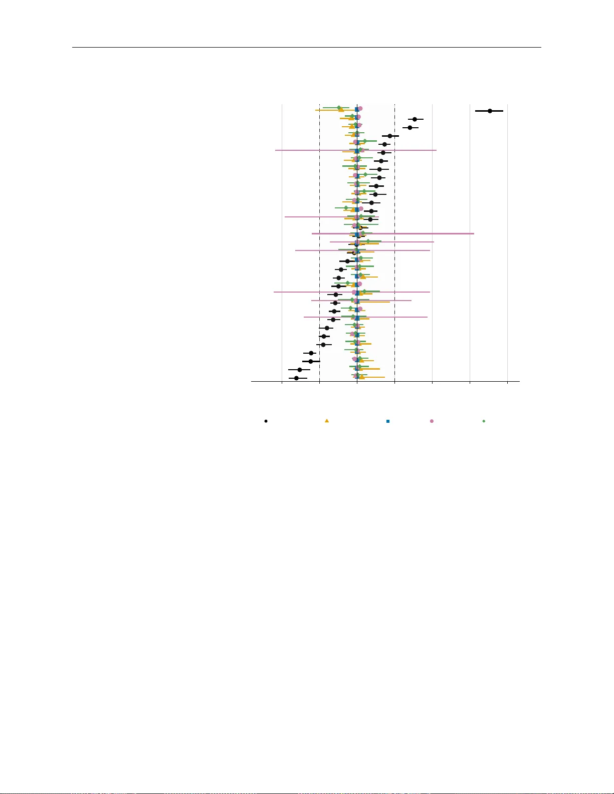
I N V E R S E P R O B A B I L I T Y W E I G H T I N G O F C O U N T E X P O S U R E S I N T H E P R E S E N C E O F M I S S I N G D A T A : A S I M U L A T I O N S T U DY A P R E P R I N T Martin N. Danka 1,2,* Jessica K. Bone 2 George B. Ploubidis 1 Richard J. Silv erwood 1 March 26, 2026 1 Centre for Longitudinal Studies, UCL Social Research Institute, Univ ersity College London 2 Research Department of Behavioural Science and Health, Institute of Epidemiology and Health Care, Uni versity College London * Corresponding author: martin.danka.21@ucl.ac.uk 0000-0003-0302-238X A B S T R AC T In verse probability of treatment weighting (IPTW) is widely used to estimate causal effects, but guidance is limited for count exposures. It is also unclear how IPTW performs when combined with multiple imputation in this conte xt. In this study , we e valuated ﬁ ve IPTW methods applied to count exposures: multinomial binning, parametric and non-parametric covariate balancing propensity scores (CBPS, npCBPS), generalised boosted models (GBM), and energy balancing. Our simulations were informed by an example using data from the 1970 British Cohort Study , aiming to estimate the effect of psychological distress, measured as a count of symptoms at age 34, on self-reported longstanding illness at age 42. W e compared these approaches on bias, co verage, ef fectiv e sample size, and other metrics under truncated negati ve binomial and Poisson e xposure distributions. W e also assessed the performance of Rubin’ s rules under dif ferent missingness mechanisms. Under complete data, multinomial, CBPS, GBM, and energy weights produced lo w bias and near -nominal coverage, whereas npCBPS resulted in bias and poor coverage due to extreme weights. When data were missing completely at random, similar performance patterns were observed for IPTW with multiple imputation. Under missing at random, bias increased with higher missingness, b ut this was present for both IPTW and co variate-adjusted regression, possibly reﬂecting a limitation of the imputation model rather than a failure of IPTW . Ov erall, these ﬁndings support the use of multinomial, CBPS, GBMs, and ener gy weights for count exposures in similar settings while highlighting trade-offs between these methods and the need for imputation models accommodating right-truncated ov erdispersed counts. Keyw ords iptw · propensity score · count data · multiple imputation · confounding IPTW of Count Exposures in the Presence of Missing Data A P R E P R I N T 1 Background Observational datasets are a valuable resource for addressing causal questions related to health, with the potential to generate evidence from real-world settings. Y et, answering these questions is more challenging in the absence of randomisation, because associations between the exposure and the outcome may lack causal interpretation due to confounding. Confounders are common causes of the exposure and the outcome, and when they are kno wn and measured, statistical approaches can be used to reduce confounding bias. T o reduce confounding due to measured v ariables, analysts typically rely on a working model of the data-generating process. Regression adjustment is a widely used approach, in which a regression model expresses the outcome as a function of the e xposure and (potential) confounders. V alid adjustment therefore depends on ho w well this outcome model is speciﬁed. Ho we ver , in some settings the analyst ma y be more willing to specify how confounders relate to the exposure mechanism, for example when outcomes are rare or otherwise challenging to model, or in outcome-wide analyses. 1 In such cases, propensity score methods offer a compelling alternative to regression adjustment. The propensity score represents the probability of receiving an e xposure level of interest gi ven a person’ s cov ariate proﬁle. Methods based on the propensity score aim to balance measured confounders across the exposure distribution, thereby approximating the balancing property of randomisation. 2 Building on the propensity score, in verse probability of treatment weighting (IPTW) is a popular method for estimating causal ef fects under confounding. This approach assigns each individual a weight inv ersely proportional to their propensity score, which aims to approximate a pseudopopulation where the exposure is independent of the observ ed confounders. The effect of interest can be estimated by implementing these weights through parametric approaches, such as weighted regression, or , less commonly , through non-parametric methods. 3 While IPTW is often applied to binary exposures, the procedure may be generalised to accommodate a range of distributions, including multicate gorical and numeric exposures. 3;4 Howe ver , the estimation of weights for numeric exposures may be complex due to their div erse distributional characteristics, making correct exposure model speciﬁcation more challenging. For this reason, weight estimation approaches that relax or avoid strict e xposure model assumptions are particularly appealing in this setting. These include approaches based on binning the exposure, 5 directly optimising cov ariate balance, 6;7 using machine learning to ﬂexibly model the e xposure-cov ariate relationships, 8 and, more recently , minimising broader measures of dependence between exposure and co variates. 9–11 Despite these adv ancements, there is a notable gap in the application of IPTW to count e xposures, which are prev alent in real-world settings. Count exposures, such as the number of hospital visits, medication doses, or symptom occurrences, are numeric exposures that take discrete, non-negati ve integer values, and, in many applications, are observed ov er only a small set of values. Their distributions may also be ov erdispersed, zero-inﬂated, or truncated. The distributional characteristics of counts may be challenging to accommodate in the IPTW framework, and approaches that av oid strict modelling assumptions are a compelling option. Ho wev er, although some of these methods have been studied for similar distributions, 5;12 they were neither de veloped nor tested speciﬁcally for count exposures, and their appropriateness remains unclear in this context. A further practical challenge for implementing IPTW is the pervasi veness of missing data in real-world datasets. When the probability of missingness giv en the observed data does not depend on any unobserved v ariables, the missing data mechanism is classiﬁed as missing at random (MAR). Under MAR, multiple imputation (MI) is a popular approach to mitigate bias that may arise when analyses are restricted to complete cases. IPTW can be incorporated in the MI framew ork using the ‘within-imputation’ approach, where weights and effects are estimated separately within each imputed dataset, follo wed by pooling of the point estimates. 13–16 . Howe ver , simulation evidence lar gely comes from studies of binary exposures, so it remains unclear how well this strategy e xtends to count exposures. Additionally , little is known about the behaviour of ﬂexible weight-construction approaches within this framework, thus limiting their applicability in real-world datasets. T o address these gaps, this study aims to in vestigate the performance of IPTW for count exposures with binary outcomes, e valuating ﬁve different approaches for weight estimation: a multinomial binning approach, parametric and non-parametric cov ariate balancing propensity scores (CBPS, npCBPS), generalised boosted models (GBM), and energy balancing. The second aim is to ev aluate ho w these IPTW methods perform under missing data conditions when combined with MI using the ‘within-imputation’ approach. This simulation study adheres to the ADEMP[I] 2 IPTW of Count Exposures in the Presence of Missing Data A P R E P R I N T framew ork. 17 Our simulations were informed by a real-world e xample, estimating the effect of psychological distress symptom counts on the risk of self-reported longstanding illness in midlife. The article is structured as follows. W e begin by introducing IPTW notation and describing the ﬁv e weight construction approaches considered in this study . W e then describe the motiv ating example that informed the simulations. Next, we outline the simulation study design and report simulation results. W e then return to the moti v ating cohort data to illustrate ho w the methods can be applied in practice. Finally , we interpret the ﬁndings and discuss implications and limitations. 2 In verse Probability of T r eatment W eighting Central to IPTW is the concept of the propensity score, which we introduce before discussing IPTW and the weight estimation methods. Our aim is not to provide a detailed description of each method, but rather to gi ve intuition, notation, and references for readers interested in further details. Throughout the manuscript, we assume that the exposure is not randomised, and we use the terms ‘exposure’ and ‘treatment’ interchangeably . 2.1 The propensity scor e Let A represent a binary exposure, taking values a ∈ { 0 , 1 } . For each a , let Y ( a ) denote the potential outcome that would be observed if, possibly counter to fact, A = a . C stands for a vector of baseline covariates, and we assume C satisﬁes the assumption of conditional exchangeability , Y ( a ) ⊥ A | C . Then, the propensity score e ( c ) is the conditional probability of being exposed gi ven the cov ariate proﬁle 2 : e ( c ) = Pr( A = 1 | C = c ) This propensity score can be estimated using both non-parametric and parametric approaches. A common approach is to model the binary exposure as a function of the covariates using logistic regression, where the propensity score is estimated by the predicted probabilities. The estimated propensity score can be used to adjust for differences in cov ariate distributions between treatment groups, thereby mimicking the conditions of a randomised experiment. This can be achiev ed through stratiﬁcation on the score, matching individuals with similar scores, or weighting, which is the focus of this paper . The propensity score has later been generalised to other exposure distributions. 4;18 T o describe this, we now allo w A to denote a generic exposure taking values a in a set Ψ (which may be discrete or continuous). The generalised propensity score is deﬁned as the conditional probability mass or density function of A gi ven the cov ariates: r ( a, c ) = f A | C ( a | c ) , a ∈ Ψ , where f A | C denotes the conditional probability mass function (for discrete A ) or probability density function (for continuous A ) of A giv en C = c . In the binary case with A ∈ { 0 , 1 } , the standard propensity score is recovered as e ( c ) = r (1 , c ) . 2.2 Exposure weights W e now gi ve an overvie w of IPTW , following the formulation of Robins, Hernán, and Brumback. 3 IPTW assigns each individual a weight in versely proportional to the propensity score. For binary exposures, the weights are determined as follows: w =        1 e ( c ) if A = 1 , 1 1 − e ( c ) if A = 0 . Assigning weights in this manner ensures that, giv en each person’ s covariate proﬁle, individuals underrepresented in their exposure group are upweighted, whereas overrepresented indi viduals are downweighted. Re-weighting in this way approximates a pseudopopulation where A ⊥ C , thus confounding is removed. 3 IPTW of Count Exposures in the Presence of Missing Data A P R E P R I N T More generally , the weights can also be derived from the generalised propensity score: w = 1 r ( a, c ) = 1 f A | C ( a | c ) In practice, the in verse probability weights can be unstable if some indi viduals have very small estimated propensity scores. A common modiﬁcation is to use stabilised weights, which replace the numerator with the marginal probability (or density) of the observed e xposure, denoted f A ( a ) 19 : w s = f A ( a ) f A | C ( a | c ) , Under the identifying assumptions of conditional exchangeability , positi vity , consistency , and no interference, 20 these exposure weights can be used to estimate a verage mar ginal causal effects. For a binary exposure, the average treatment effect ( AT E ), is deﬁned as AT E = E { Y (1) } − E { Y (0) } . The non- parametric IPTW estimator for the AT E replaces mean potential outcomes with weighted av erages of the observ ed outcomes for the exposed and une xposed: d A TE IPTW = b E { Y (1) } − b E { Y (0) } = P n i =1 w i Y i A i P n i =1 w i A i − P n i =1 w i Y i (1 − A i ) P n i =1 w i (1 − A i ) . For a non-binary e xposure (including counts), IPTW can target the a verage (marginal) dose-response function µ ( a ) = E { Y ( a ) } , 4 and this can be used to deﬁne a verage causal ef fects as contrasts µ ( a ) − µ ( a ′ ) between two e xposure le vels a and a ′ . The dose-response can be expressed using a marginal structural model, 3 µ ( a ) = E { Y ( a ) } = m ( a ; δ ) , where m ( · ) is a chosen working model (for e xample, linear, spline-based, or categorical in a ). The parameters δ can then be estimated using IPTW , typically by ﬁtting an outcome model re-weighted by the in verse probability weights. If the marginal structural model is linear, E { Y ( a ) } = δ 0 + δ 1 a , the dose-response has a constant slope, so that δ 1 represents a constant av erage change in µ ( a ) per one-unit increase in A . Other causal effects, such as the marginal risk or odds ratio, can be expressed in a similar manner . 21 In practice, IPTW can be challenging to implement for numeric exposures due to its sensitivity to model misspeciﬁcation, as both the conditional and marginal mass or density functions for stabilised weights must be correctly speciﬁed, and extreme weights are a common issue e ven after stabilisation. While this issue is not speciﬁc to counts, it is ampliﬁed by the challenges of specifying discrete distributions that accommodate ov erdispersion, truncation, zero inﬂation, and other features. Sev eral alternativ es relax this parametric assumption, which we explore further . 2.3 Binning approaches Multicategorical exposures can be modelled directly using multinomial or ordinal regression, which allows the deriv ation of stabilised exposure weights. This approach can be extended to numeric exposures by ﬁrst grouping A into K categories (e.g. using quantiles or theory-driven cut–points) and then modelling the resulting multicategory exposure. 5 Using multinomial regression, the denominator of the stabilised weight for an indi vidual with exposure le vel A = k and cov ariates C = c is the estimated conditional probability ˆ f A | C ( k | c ) = Pr( A = k | C = c ) = exp { ˆ β 0 k + c ⊤ ˆ β k } P K j =1 exp { ˆ β 0 j + c ⊤ ˆ β j } . The numerator of the stabilised weight is the estimated marginal probability of receiving e xposure level k , ˆ f A ( k ) = c Pr( A = k ) . 4 IPTW of Count Exposures in the Presence of Missing Data A P R E P R I N T 2.4 Covariate balancing appr oaches The propensity score has a dual role: it represents the conditional probability of receiving a gi ven e xposure lev el gi ven cov ariates, and, under correct model speciﬁcation, it also acts as a balancing score, meaning the resulting weights balance the distribution of cov ariates across exposure le vels. 2 The co variate balancing propensity score (CBPS) methods exploit this dual role, attempting to ﬁnd propensity scores or weights optimised on this balancing property . 6;7 For count e xposures, we consider the extension by F ong et al., 6 originally proposed for continuous treatments. The exposure A is ﬁrst standardised to A ∗ i , and cov ariates are centred and orthogonalised to giv e C ∗ i , so the stabilised weight for each individual tak es the form: w i = f A ∗ ( A ∗ i ) f A ∗ | C ∗ ( A ∗ i | C ∗ i ) CBPS then uses constrained optimisation to identify weights w i that satisfy a balancing constraint: N X i =1 w i A ∗ i C ∗ i = 0 , so that, in the weighted sample, the standardised exposure and co variates are uncorrelated. This generalisation of the CBPS can be employed parametrically or non-parametrically . In the parametric version, the marginal density f A ∗ is assumed to be standard normal, and f A ∗ | C ∗ is a conditional normal density obtained from a linear regression of A ∗ on C ∗ . The regression parameters are estimated by solving a system of equations that combines (i) a standard normal–re gression condition for the residual v ariance with (ii) the cov ariate balancing condition abov e, which can be vie wed as an application of the generalised method of moments. Because estimation e xplicitly targets balance rather than only model ﬁt, we expect this approach to retain some rob ustness to misspeciﬁcation of the parametric model and marginal distrib ution for A , making the approach potentially applicable to count exposures provided that balance is achie ved. The non-parametric implementation (npCBPS) does not require specifying the distributional form of f A ∗ or f A ∗ | C ∗ . Instead, it uses constrained optimisation to directly ﬁnd positiv e weights w i that meet the balancing condition abo ve and also satisfy additional constraints capturing desirable properties of stabilised weights. In the weighted sample, the standardised exposure and co variates retain their mar ginal means (that is, zero), and the total weight equals N : N X i =1 w i C ∗ i = 0 , N X i =1 w i A ∗ i = 0 , N X i =1 w i = N , w i > 0 for all i. Among the weight vectors satisfying these constraints, npCBPS uses an empirical likelihood criterion to identify weights that are, as far as the constraints allow , close to equal (i.e. each w i close to 1), thereby attempting to avoid ov erly extreme weights. 2.5 Generalised boosted models Generalised boosted models (GBMs) use the gradient boosting algorithm to ﬂe xibly estimate regression functions. 22 They can be used to estimate the exposure–confounder relationships, and thus estimate the propensity score and exposure weights. 23;24 W e consider the extension that was originally proposed for continuous exposures by Zhu et al. 8 In this context, a commonly used working model for the generalised propensity score assumes a linear mean function A i = C ⊤ i β + ε i , ε i ∼ N (0 , σ 2 ) , so that the conditional density f A | C ( A i | C i ) can be obtained from a normal model, and the mar ginal density f A ( A i ) can be speciﬁed parametrically or estimated by kernel density estimation. GBMs replace the linear predictor with a ﬂexible, non-parametric re gression function A i = m ( C i ) + ε i , 5 IPTW of Count Exposures in the Presence of Missing Data A P R E P R I N T where m ( C i ) is represented as a sum of simple re gression trees. Each tree partitions the cov ariate space into regions R bj and assigns a constant prediction c bj within each region, so that m ( C i ) = m 0 + M X b =1 K b X j =1 c bj I { C i ∈ R bj } , with m 0 the initial mean of A , M the total number of trees, K b the number of terminal nodes (re gions) in tree b , and I { C i ∈ R bj } an indicator that observation i falls in region R bj . The algorithm starts from m 0 and then adds trees sequentially , each ﬁt to the current residuals (pseudo-residuals), so that each c bj acts as a small correction to the current ﬁt in region R bj . The number of trees M controls the complexity of the model. In standard applications, M can be chosen by cross- validation. For propensity score estimation, GBMs are instead tuned to optimise cov ariate balance in the weighted sample. For binary exposures, one can stop boosting at the iteration that minimises the a verage standardised absolute mean dif ference in cov ariates between exposure groups. For continuous exposures, M can be chosen to minimise the av erage absolute weighted correlation between the exposure and the co v ariates. 2.6 Energy balancing While the pre viously discussed methods either relax or are robust to certain restricti ve parametric assumptions, the y nonetheless require in vestigators to choose which moments of the covariates and e xposure should be decorrelated, and there are no established guidelines for making this choice. Energy balancing relies on energy distance-based metrics, enabling researchers to circumvent the need to pre-specify particular moments for decorrelation. Intuitiv ely , energy distance quantiﬁes how (dis)similar two distrib utions are by comparing average pairwise distances within observations drawn from the same distrib ution with those between observations from dif ferent distributions. It is zero when the two distributions are identical and increases as the y di ver ge, capturing differences not only in means b ut also in higher-order moments. 10 Building on this metric, Huling and Mak 25 proposed energy balancing for binary exposures, which uses constrained optimisation to ﬁnd weights that minimise the energy distance between the weighted covariate distribution in each exposure group and the cov ariate distrib ution in the ov erall sample. This idea was e xtended to continuous exposures, deﬁning independence weights (also called distance cov ariance optimal weights). 11 In this setting, the weights are obtained by minimising a criterion that combines (i) a weighted distance cov ariance term V 2 n, w ( C , A ) , which is equal to zero if the exposure A and cov ariates C are independent under the weights, and (ii) two energy distance terms E { F n C , w , F n C } and E { F n A, w , F n A } that penalise departures of the weighted marginal distrib utions of A and C from their original empirical marginals. Formally , the weights w minimise a criterion of the form: D ( w ) = V 2 n, w ( C , A ) + E { F n C , w , F n C } + E { F n A, w , F n A } , The optimisation is carried out subject to w i ≥ 0 and P N i =1 w i = N , so that the a verage weight is 1. As with CBPS and npCBPS, these constraints yield stabilised weights by construction. 3 Motivating example W e now introduce the moti vating example, which reﬂects some of the methodological challenges faced when applying IPTW to counts. The data come from the 1970 British Cohort Study (BCS70). BCS70 is a multidisciplinary birth cohort of ov er 17,000 indi viduals born in a single week in 1970 in England, Scotland, and W ales, with 11 completed sweeps of data collection to date. Further details are av ailable in the cohort proﬁles 26;27 and on the Centre for Longitudinal Studies website ( https://cls.ucl.ac.uk/cls- studies/1970- british- cohort- study/ ). Across multiple data collection sweeps, participants completed the Malaise Inv entory , a measure of psychological distress. A nine-item version was introduced at age 34 (2004 sweep), with binary (‘yes’/‘no’) responses to symptoms such as worrying often, feeling miserable or depressed, and feeling tired most of the time, yielding a symptom count ranging from 0 to 9. Previous work has demonstrated scalar in variance of this shortened measure across time, cohorts, and gender in UK birth cohorts. 28;29 At age 42 (2012 sweep), participants were asked a series of questions about their 6 IPTW of Count Exposures in the Presence of Missing Data A P R E P R I N T health. For simplicity in this motiv ating example, we focus on a single broad binary indicator of having a longstanding illness. This was marked as present if a participant answered ‘yes’ to having “any physical or mental health conditions or illnesses lasting or expected to last 12 months or more". Our aim is to estimate the ef fect of psychological distress at age 34 on the presence of longstanding illness at age 42 (2012 sweep). This relationship is likely confounded by many inﬂuences, with many potential confounders av ailable in the dataset, as outlined in T able S1 in the Supplementary Information. These include prior health and health behaviours (for example, past longstanding illness, physical acti vity), adult socioeconomic situation (occupation and income), sociodemographic characteristics (sex at birth, partnership), and early-life and developmental inﬂuences (including parental social class, ov ercro wding, housing tenure, parental education and income, birthweight, maternal smoking in pregnanc y , childhood cognition, and adolescent psychological distress). The estimand is the causal risk ratio (RR), and we wish to estimate this using IPTW . W e focus on the target population of individuals born in 1970 in England, Scotland, or W ales, who remained alive and did not emigrate by age 42. This problem is further used to inform the simulation design. 4 Simulation study design 4.1 Data-generating mechanisms T o ev aluate the performance of the ﬁve IPTW approaches with count exposures, we began by generating 2,000 datasets, each having 5,000 observ ations. The number of repetitions was determined to giv e about 0.005 Monte Carlo standard error (SE) on cov erage. 17 Three covariates C 1 , C 2 and C 3 were sampled from a multiv ariate normal distribution C ∼ N ( 0 , Σ ) , where the diagonal elements (the v ariances) were set to Σ ii = 1 and the off-diagonal elements (corresponding to pairwise correlations) to Σ ij = 0 . 3 for all i  = j . After sampling, C 1 was dichotomised by setting it to 0 where C 1 ≤ 0 and to 1 where C 1 > 0 , to keep the proportions approximately equal to 0 . 5 , resulting in a variable resembling sex at birth in cohort datasets. C 2 and C 3 were retained as continuous variables. Exposure A was generated under two data-generating mechanisms (DGMs). The ﬁrst mechanism aimed to produce a truncated conditional negati ve binomial distrib ution, moti vated by the Malaise In ventory , using minimal adjustments to av oid overreliance on the speciﬁc characteristics of the moti vating example. The second mechanism focused on a truncated conditional Poisson distribution with similar properties but no o verdispersion. The expected count for each observation w as gi ven by λ i = exp( β 0 + β 1 C i, 1 + β 2 C i, 2 + β 3 C i, 3 ) where β 0 = ln 1 . 5 was chosen pragmatically to generate a marginal exposure distribution broadly similar to that observed for the Malaise Inv entory at age 34 in BCS70 (mean count 1 . 7 ), and β 1 = 0 . 4 , β 2 = 0 . 1 , and β 3 = 0 . 1 to keep most counts within close ranges. Under the ﬁrst DGM, the exposure v ariable was then sampled from a negati ve binomial distribution A ∼ N eg B in ( λ i , k ) , with the dispersion parameter set to the observed mar ginal ˆ k = 1 . 3 of the Malaise In ventory at age 34 in BCS70. The second mechanism used the same model but simulated A ∼ P ois ( λ i ) . Because count distrib utions are often truncated in real-world datasets, we emplo yed a rejection sampling procedure, resampling all A i > 10 under both mechanisms. The exposure and cov ariates were then used to simulate a binary outcome Y . The conditional probability of Y was expressed using a log-binomial model: ln π i = γ 0 + γ 1 A i + γ 2 C i, 1 + γ 3 C i, 2 + γ 4 C i, 3 Here, γ 0 = ln 0 . 03 , setting the baseline probability to 3% to roughly reﬂect the pre valence of coronary heart disease in England in 2023. 30 . The cov ariate effects were set to γ 2 = ln 1 . 4 and γ 3 = γ 4 = ln 1 . 1 . The dose-response ef fect of interest was v aried across the values γ 1 ∈ { ln 1 . 0 , ln 1 . 1 , ln 1 . 2 } . The cov ariate coef ﬁcients and the intercept were selected to keep π i < 1 for all i , which was empirically veriﬁed for all simulated datasets. The outcome was then simulated as Y i ∼ B er noul li ( π i ) . 7 IPTW of Count Exposures in the Presence of Missing Data A P R E P R I N T 4.2 Missing data mechanisms T o introduce missing data, we ﬁrst simulated complete datasets and then induced missingness by amputation. 31;32 W e aimed to approximate a scenario commonly observ ed in birth cohorts, including BCS70, where missingness tends to increase progressi vely with each sweep of data collection. W e therefore introduced missing data in the confounders C 2 and C 3 , the exposure A , and the outcome Y , while the binary confounder C 1 remained fully observed, resembling a baseline variable such as sex at birth that is typically known for all cohort members. The per-v ariable probability of missingness p i was speciﬁed to increase in the order p C 2 < p C 3 < p A < p Y . W e also aimed to control the ov erall lev el of missingness, deﬁned as the probability that an indi vidual has at least one missing value, denoted by ϕ . W e considered three target o verall le vels of missingness, ϕ ∗ ∈ { 0 . 20 , 0 . 40 , 0 . 60 } , across two scenarios, MCAR and MAR. Under MCAR, the variables C 2 , C 3 , A , and Y were independently set to missing with variable-speciﬁc probabilities p i , i = 1 , . . . , 4 , ordered as abo ve. The ov erall missingness probability under MCAR is ϕ MCAR = 1 − 4 Y i =1 (1 − p i ) . W e imposed a simple linear structure p i = p 0 + ( i − 1) d, i = 1 , . . . , 4 , with p 0 ≥ 0 , d ≥ 0 and p 0 + 3 d < 1 , so that the marginal proportion of missingness increased across variables. T o ensure we controlled both the per -variable p i and the ov erall ϕ , we used constrained optimisation to select ( p 0 , d ) so that the av erage realised ¯ ϕ ≈ ϕ ∗ , minimising ( ¯ ϕ − ϕ ∗ ) 2 . Under MAR, we again allowed C 2 , C 3 , A , and Y to be missing but now generated missingness indicators from logistic models in which missingness depended on the remaining v ariables. Let M ij = 1 if v ariable i is missing for indi vidual j and 0 otherwise. For simplicity , we omit the individual index j and write M i for the missingness indicator of variable i , so that p i = E ( M i ) . The missingness mechanisms were speciﬁed as logit { Pr( M C 2 = 1 | C 1 ) } = γ 0 ,C 2 + C 1 , logit { Pr( M C 3 = 1 | C 1 , C 2 ) } = γ 0 ,C 3 + C 1 + C 2 , logit { Pr( M A = 1 | C 1 , C 2 , C 3 ) } = γ 0 ,A + C 1 + C 2 + C 3 , logit { Pr( M Y = 1 | C 1 , C 2 , C 3 , A ) } = γ 0 ,Y + C 1 + C 2 + C 3 + A. The intercepts γ 0 ,i control the mar ginal missingness probabilities p i = E ( M i ) , but because the M ij are no w dependent, the ov erall missingness rate under MAR, ϕ MAR = 1 − E n 4 Y i =1 (1 − M i ) o , is no longer equal to 1 − Q i (1 − p i ) . Therefore, to impose the same linear progression p i = p 0 + ( i − 1) d while maintaining the target ϕ ∗ , we used constrained optimisation with a Monte Carlo approximation to the MAR objecti ve: for a candidate ( p 0 , d ) , we (i) solv ed for γ 0 ,i that yielded the requested p i and (ii) e valuated ˆ ϕ MAR empirically in a ﬁxed lar ge simulated sample ( N = 1 , 000 , 000 ). W e then chose ( p 0 , d ) to make ˆ ϕ MAR ≈ ϕ ∗ . Full details are provided in the Supplementary Information, with parameter values in T able S2. 4.3 Effect and weight estimation The estimand of interest w as the ln RR per unit increase in the e xposure. This was estimated using a Poisson re gression model for the outcome, using a sandwich estimator for variance (a procedure known as modiﬁed Poisson re gression). 33 The model was reweighted using stabilised treatment weights. W e compared ﬁve methods for constructing these weights: binning with weights constructed via a multinomial model (further referred to as ‘multinomial weights’), 8 IPTW of Count Exposures in the Presence of Missing Data A P R E P R I N T CBPS, npCBPS, GBM, and energy balancing (distance cov ariance optimal weights). For each weighting method, analyses were conducted using both the estimated stabilised treatment weights and a winsorised v ersion of these weights, with winsorisation at the 99th percentile. T o provide a comparison against a method with kno wn properties, we also estimated the ef fect using unweighted regression with simple cov ariate adjustment. Lastly , we provide results for the unadjusted regression model, without an y account for confounding, for further comparison. The weighting methods were implemented using the WeightIt R package. 34 The package implementations of the methods broadly match the descriptions in Section 2, with a few practical details noted here. Prior to ﬁtting the multinomial model to derive weights, we identiﬁed exposure lev els with individual prev alence belo w 1% in each simulated dataset. Whenev er this occurred, the af fected le vels were conﬁned to the e xtreme upper tail of the exposure distribution. These le vels were then combined to a void sparse multinomial categories. The exposure w as only binned this way for constructing the multinomial weights, but the original count exposure entered the (re-weighted) model for ef fect estimation. In the WeightIt implementation of CBPS, the mar ginal exposure mean and v ariance enter the moment conditions as parameters rather than being ﬁxed to their observed values. For GBMs, the algorithm was similar to that described in Zhu et al., 8 with two modiﬁcations to the balance-based stopping rule. First, the criterion was set to minimise the root-mean-squared absolute weighted correlation instead of the a verage absolute weighted correlation between the exposure and cov ariates, thus lar ger imbalances were penalised more strictly . Second, the default WeightIt implementation computes this correlation in the full sample rather than using a bootstrap-based estimate. For incomplete datasets, missing data were handled using MI by chained equations. All analysis v ariables were included in the imputation models. The continuous and count-type v ariables ( C 2 , C 3 , A ) were imputed using predicti ve mean matching, and the binary outcome Y was imputed using logistic regression, as implemented in the mice R package. 35 In line with general recommendations, the number of imputations w as chosen to equal the realised ϕ r × 100 in each simulated dataset. 36 The imputed datasets were analysed using the ‘within-imputation’ approach, combining point estimates and sandwich variances using Rubin’ s rules. 37 T o reduce computational burden, analyses under missing data were only conducted for the DGMs with true RR = 1.1. 4.4 Perf ormance metrics The primary metrics of interest were bias and co verage, although empirical and model-based SE were also provided, following deﬁnitions in Morris et al. 17 W eighting methods may produce large weights, with reduced precision being the potential consequence. Effecti ve sample size (ESS) is a commonly used summary of this loss of precision, representing the size of a hypothetical unweighted sample that would provide the same precision as the weighted sample. This is obtained as E S S = ( P w ) 2 P w 2 , where w stands for the weights. 23;38 In this study , we provided the av erage ESS for each method across the simulated datasets, its standard deviation, and the 5th and 95th percentiles. T o assess if the weights successfully decorrelated the treatment and the co v ariates, we provided metrics based on the absolute weighted treatment-cov ariate Pearson (or point-biserial) correlations, 39 av eraged across the three cov ariates in each dataset. Additionally , the dependence metric was used as a composite summary of the weights, providing a relativ e comparison of how well different methods reduced residual dependence between A and C while preserving the original marginal distributions. Lower values of the dependence metric indicate better-performing weights. W e also reported the energy-distance components separately to assess deviations from the original marginal distrib utions of A and C . 11 Because some methods optimise directly on these metrics, the y were not used as evidence of superior performance for those methods. The simulations were conducted in R v4.4 under the UCL Myriad High Performance Computing facility . W e also assessed the computational speed of each weighting method locally , summarising the relative time required for weight estimation ov er 20 simulated datasets. Further details of the simulation implementation and the computation time assessment are provided in the Supplementary Information. 9 IPTW of Count Exposures in the Presence of Missing Data A P R E P R I N T 0.0 0.1 0.2 0.3 0 2 4 6 8 10 Relative frequency Obser ved Malaise score (BCS70) A 0.0 0.1 0.2 0.3 0 2 4 6 8 10 Simulated e xposure (NegBin) B 0.0 0.1 0.2 0.3 0 2 4 6 8 10 Exposure Simulated e xposure (P oisson) C Figure 1: Histograms of the Malaise score and the simulated exposures. A , Observed Malaise score at age 34 in the 1970 British Cohort Study (N = 9 596; range 0–9). B , Simulated exposure (N = 1,000,000) from a conditional negati ve binomial distribution, truncated by resampling values greater than 10. C , Simulated exposure (N = 1,000,000) from a conditional Poisson distribution, truncated by resampling values greater than 10. BCS70 – 1970 British Cohort Study; NegBin – Ne gati ve Binomial. 5 Simulation results 5.1 Simulated datasets T o approximate and further characterise the distributions implied by each DGM, we generated a large sample of 1,000,000 observations. The achie ved marginal distribution of the simulated truncated negati ve binomial exposure yielded the av erage count of 1.81 (SD = 2.04, Mdn = 1.00, IQR from 0 to 3, overdispersion parameter k = 1.30, panel B of Figure 1), which was similar in location and scale to that of Malaise In ventory (M = 1.7, SD = 1.90, Mdn = 1.00, IQR 0 to 3, overdispersion parameter k = 1.29, panel A of Figure 1). The marginal truncated Poisson distribution had an av erage count of λ = 1.91 (SD = 1.49, Mdn = 2.00, IQR 1to 3, panel C of Figure 1). Most exposure values remained within the pre-speciﬁed range ( ≤ 10), with only 0.9% v alues truncated via resampling for the negati ve binomial e xposure and fe wer than 0.01% for the Poisson e xposure. When the true RR was 1.10, the mar ginal prev alence of the simulated outcome was 4.5% for both the negati ve binomial and Poisson exposures. The confounded RR per unit increase in the exposure was 1.13 under the ne gative binomial e xposure and 1.17 under the Poisson exposure. 5.2 Perf ormance under complete data Our simulations produced comparable results for all metrics across the three effect sizes. Therefore, unless otherwise stated, we present results for the scenario in which the true unconfounded RR = 1.1. An interactiv e table of all results can be found at martindanka.github.io/iptw- sim- shinylive/ . † Performance metrics under no missingness are shown in T able 1. CBPS, energy weights, GBM, and multinomial weights all demonstrated good performance across the two exposure DGMs in terms of low bias (absolute value of relativ e bias below 3%). In contrast, npCBPS underestimated the true effect, with relati ve bias amounting to -15.2% of the true effect for the negati ve binomial exposure and -26.1% for the Poisson exposure. The sandwich variance estimator also provided near -nominal cov erage for all methods with lo w bias. W insorisation of weights at the 99 th percentile had relati vely modest impact on performance. For multinomial, CBPS, GBM and energy weights, winsorisation led to slightly lar ger bias, particularly under the Poisson exposure DGM where relativ e bias ranged from 6.3% to 8.4%. Cov erage for these methods remained near the nominal v alue, with slightly smaller standard errors compared with raw weights. For npCBPS, winsorisation reduced the magnitude of bias and improv ed cov erage, b ut performance remained worse than for the other weighting schemes (relati ve bias of 3.5% for the negati ve binomial and 19.7% for the poisson DGM). † Please note that the application may require sev eral minutes to load on ﬁrst use. 10 IPTW of Count Exposures in the Presence of Missing Data A P R E P R I N T T able 1: Performance metrics for the simulations under complete data and RR = 1.1 Raw weights Winsorised weights (99 th percentile) Method Bias (MCSE) Rel. Bias (MCSE) Emp. SE Model SE Coverage (MCSE) Bias (MCSE) Rel. Bias (MCSE) Emp. SE Model SE Coverage (MCSE) Negative binomial exposur e Unadjusted 0.026 (0.001) 27.1 (0.6) 0.026 0.026 0.811 (0.009) — — — — — Adjusted -0.001 (0.001) -0.9 (0.6) 0.028 0.027 0.953 (0.005) — — — — — Multinomial -0.001 (0.001) -1.0 (0.7) 0.032 0.031 0.950 (0.005) 0.003 (0.001) 2.9 (0.7) 0.030 0.029 0.951 (0.005) CBPS -0.002 (0.001) -2.2 (0.7) 0.032 0.031 0.951 (0.005) 0.002 (0.001) 2.0 (0.7) 0.030 0.030 0.952 (0.005) npCBPS -0.014 (0.001) -15.2 (1.2) 0.051 0.041 0.892 (0.007) 0.003 (0.001) 3.5 (0.7) 0.030 0.029 0.950 (0.005) GBM -0.001 (0.001) -1.0 (0.8) 0.033 0.032 0.937 (0.005) 0.003 (0.001) 3.3 (0.7) 0.030 0.030 0.947 (0.005) Energy -0.001 (0.001) -1.3 (0.8) 0.036 0.035 0.946 (0.005) 0.002 (0.001) 1.7 (0.8) 0.034 0.034 0.948 (0.005) Poisson exposur e Unadjusted 0.060 (0.001) 63.3 (0.9) 0.038 0.039 0.643 (0.011) — — — — — Adjusted 0.000 (0.001) -0.5 (1.0) 0.042 0.043 0.944 (0.005) — — — — — Multinomial -0.001 (0.001) -1.5 (1.3) 0.057 0.055 0.939 (0.005) 0.008 (0.001) 8.4 (1.1) 0.048 0.048 0.945 (0.005) CBPS -0.001 (0.001) -1.5 (1.3) 0.057 0.054 0.944 (0.005) 0.007 (0.001) 7.2 (1.1) 0.048 0.048 0.945 (0.005) npCBPS -0.025 (0.002) -26.1 (2.4) 0.102 0.073 0.901 (0.007) 0.019 (0.001) 19.7 (1.1) 0.046 0.047 0.924 (0.006) GBM 0.000 (0.001) -0.1 (1.4) 0.059 0.056 0.940 (0.005) 0.008 (0.001) 8.3 (1.1) 0.048 0.049 0.944 (0.005) Energy -0.001 (0.001) -1.4 (1.4) 0.060 0.060 0.945 (0.005) 0.006 (0.001) 6.3 (1.3) 0.055 0.055 0.946 (0.005) Note: Entries are Monte Carlo summaries over 2,000 simulated datasets. Point estimates and conﬁdence intervals were deri ved from weighted Poisson regression models with a sandwich estimator for v ariance. Unweighted outcome regressions (adjusted and unadjusted) are shown for comparison. All IPTW methods used stabilised weights. (np)CBPS – (Non-Parametric) Covariate Balancing Propensity Scores; Emp. SE – Empirical Standard Error; GBM – Generalised Boosted Models; MCSE – Monte Carlo Standard Error; Model SE – Model-Based Standard Error; Rel. Bias – Relative Bias. 11 IPTW of Count Exposures in the Presence of Missing Data A P R E P R I N T 5.3 Properties of the weights T able 2 summarises cov ariate balance metrics and ef fectiv e sample sizes for the unwinsorised weights. Multinomial, CBPS, and GBM weights resulted only in a small loss of precision: under the negati ve binomial DGM, mean ESS ranged from 4,623 to 4,679 , with small standard deviations and 5 th percentile ESS all abov e 4,511 , close to the nominal 5,000 observ ations. Compared to these methods, energy balancing resulted in greater precision loss (mean ESS = 3,639 ). Similar patterns were observed under the Poisson DGM, although mean ESS was lower across all methods. npCBPS sho wed substantial and highly v ariable precision loss, with mean ESS of 3,243 for the negati ve binomial and 1,675 for the Poisson DGM, and v ery low ESS in some repetitions (for example, under the Poisson DGM the 5 th percentile ESS was 453). Multinomial, CBPS, GBM, and energy weights achie ved satisf actory exposure–co variate independence, with the mean absolute weighted correlation | ρ w | < 0 . 02 for each method. Under the Poisson DGM, multinomial weights yielded larger residual correlations in some repetitions, indicated by max | ρ w | = 0.12 , although such cases were rare, with 95 th percentile | ρ w | = 0.03 . npCBPS achiev ed poorer balance compared to the other methods, with lar ger mean | ρ w | and more extreme tail values. Across methods, the av erage composite dependence metric D w and energy distance metrics ϵ A and ϵ C were close to zero, suggesting that the weighting generally preserved the marginal exposure and cov ariate distributions. Howe ver , these metrics were consistently largest for npCBPS, reinforcing its comparatively poorer balance and precision. W insorising the weights maintained greater precision, as reﬂected by a higher mean ESS, but this came at the cost of reduced cov ariate balance, evidenced by an increase in the av erage absolute exposure-cov ariate correlations. 5.4 Computational speed The methods v aried in computational speed (Figure S1 in the Supplementary Information), with the CBPS method being the fastest, with a mean absolute runtime of 0.05 seconds per run under the giv en local setup. Across the 20 simulated datasets, the multinomial binning approach was, on a verage, 3.9 times slo wer than CBPS. In contrast, npCBPS was approximately 64.0 times slo wer, while GBM exhibited a relative slowdo wn of 273.0 times. Energy weights were particularly computationally intensiv e, requiring 1285.3 times longer than the multinomial weights. 5.5 Perf ormance under missing data T ables 3 and 4 present performance of the ‘within-imputation’ estimator . Under MCAR, the adjusted outcome model and the IPTW estimators based on multinomial, CBPS, GBM and energy weights maintained low bias even with a high proportion of missing data. When 60% of rows were incomplete, relati ve bias for these methods remained within ± 3% for the negati ve binomial exposure DGM and within about ± 5% for the Poisson exposure DGM. Unadjusted estimation continued to display large positiv e bias (around 28% for the negativ e binomial and 65% for the Poisson exposure at 60% missing). npCBPS sho wed persistent neg ativ e bias. Cov erage under MCAR sho wed evidence of the pooled sandwich estimator being slightly conservati ve with higher missingness across methods. Under MAR, the ‘within-imputation’ estimator sho wed increasing ne gative bias as the amount of missingness increased, particularly under the negati ve binomial DGM. At 20% of incomplete ro ws, multinomial, CBPS, and energy weights showed a small relati ve bias between -3.0% and -4.0%, depending on method, which then increased to between -13.8% and -14.8% at 60% of incomplete rows. Ho wev er, this increase in bias was also apparent for regression adjustment, demonstrating that it was not speciﬁcally due to the performance of the weighting estimators. While a similar pattern was observed under the Poisson DGM, relati ve bias was smaller , ranging from -4.1% to -4.6% across the three weighting methods. For the unadjusted method, negativ e bias from underadjustment partly counterbalanced the positive bias from increasing missingness, resulting in lower net relati ve bias at higher missingness. This bias cancellation should not be interpreted as evidence of superior performance under higher missingness. npCBPS remained the method with highest bias among the weighting estimators across all DGMs with missingness. Cov erage under MAR showed similar patterns to those under MCAR. The increased bias under MAR was not speciﬁc to the weighting methods, as it was observed for both regression adjustment and IPTW . W e therefore hypothesised that this bias may hav e arisen from the imputation procedure, particularly from imputing the count exposure A , since it was more pronounced under the neg ativ e binomial exposure than under the Poisson DGM. T o examine this, we conducted an additional sensitivity analysis in which the same ov erall 12 IPTW of Count Exposures in the Presence of Missing Data A P R E P R I N T T able 2: Cov ariate balance metrics for the simulations under complete data and RR = 1.1 Method Mean ESS SD ESS 5th perc ESS 95th perc ESS Mean D w SD D w Mean ϵ A Mean ϵ C Mean | ρ w | SD | ρ w | 95th | ρ w | Max | ρ w | Negative binomial exposur e Multinomial 4,667 62 4,558 4,746 <0.001 <0.001 <0.0001 <0.0001 0.008 0.004 0.015 0.038 CBPS 4,679 44 4,605 4,745 <0.001 <0.001 <0.0001 <0.0001 <0.0001 <0.0001 <0.0001 <0.0001 npCBPS 3,243 838 1,717 4,412 0.006 0.004 <0.001 <0.001 0.044 0.029 0.093 0.138 GBM 4,623 68 4,511 4,713 0.001 <0.001 <0.0001 <0.0001 0.011 0.005 0.020 0.034 Energy 3,639 64 3,527 3,737 <0.001 <0.0001 <0.0001 <0.0001 0.002 <0.001 0.002 0.004 Poisson exposur e Multinomial 3,909 338 3,318 4,197 <0.001 0.001 <0.0001 <0.0001 0.012 0.009 0.026 0.122 CBPS 3,975 137 3,730 4,149 <0.001 <0.001 <0.0001 <0.0001 <0.0001 <0.0001 <0.0001 <0.0001 npCBPS 1,675 1,007 453 3,589 0.012 0.010 0.001 <0.001 0.064 0.044 0.147 0.233 GBM 3,891 253 3,469 4,179 0.002 <0.001 <0.0001 <0.001 0.016 0.007 0.029 0.059 Energy 3,066 99 2,901 3,221 <0.001 <0.0001 <0.0001 <0.0001 0.003 <0.001 0.004 0.005 Note: The ϵ C metric and the absolute treatment–co v ariate correlations were a veraged across the three confounders. (np)CBPS – (Non-Parametric) Cov ariate Balancing Propensity Scores; D w – distance metric optimised by the ener gy-balancing approach; ϵ A – energy distance between the weighted and unweighted marginal distrib utions of the exposure; ϵ C – energy distance between the weighted and unweighted marginal distributions of the cov ariates; ESS – Effecti ve Sample Size; GBM – Generalised Boosted Models; ρ w – av erage weighted treatment–cov ariate correlation; perc – percentile; SD – standard deviation. 13 IPTW of Count Exposures in the Presence of Missing Data A P R E P R I N T T able 3: Relativ e bias (MCSE) under varying missingness scenarios and RR = 1.1. MCAR MAR Method Complete 20% 40% 60% 20% 40% 60% Negative binomial exposur e Unadjusted 27.1 (0.6) 27.5 (0.7) 28.0 (0.8) 27.8 (0.9) 22.1 (1.0) 14.2 (1.3) 7.7 (1.6) Adjusted -0.9 (0.6) -0.4 (0.7) 0.4 (0.8) 0.5 (0.9) -4.4 (1.0) -10.4 (1.3) -15.4 (1.7) Multinomial -1.0 (0.7) -0.1 (0.8) 1.2 (0.9) 2.0 (1.0) -3.0 (1.0) -8.7 (1.4) -14.1 (1.7) CBPS -2.2 (0.7) -1.3 (0.8) 0.0 (0.9) 0.7 (1.0) -3.8 (1.0) -9.4 (1.3) -14.4 (1.7) npCBPS -15.2 (1.2) -14.4 (1.1) -12.8 (1.1) -11.1 (1.2) -16.6 (1.3) -21.8 (1.4) -26.2 (1.7) GBM -1.0 (0.8) -0.4 (0.8) 0.7 (0.9) 1.5 (1.0) -2.8 (1.0) -8.6 (1.3) -13.8 (1.7) Energy -1.3 (0.8) -0.4 (0.9) 1.3 (0.9) 2.7 (1.0) -4.0 (1.1) -9.8 (1.4) -14.8 (1.7) Poisson exposur e Unadjusted 63.3 (0.9) 63.8 (1.0) 64.7 (1.1) 65.2 (1.3) 60.1 (1.2) 56.3 (1.5) 50.8 (2.0) Adjusted -0.5 (1.0) 0.5 (1.1) 1.8 (1.2) 3.3 (1.4) -1.6 (1.3) -2.7 (1.6) -4.4 (2.1) Multinomial -1.5 (1.3) -0.1 (1.4) 1.7 (1.5) 3.2 (1.6) -1.6 (1.5) -2.7 (1.8) -4.6 (2.2) CBPS -1.5 (1.3) -0.1 (1.4) 1.2 (1.4) 2.6 (1.6) -1.5 (1.5) -2.5 (1.8) -4.6 (2.2) npCBPS -26.1 (2.4) -22.1 (2.2) -19.3 (2.1) -19.0 (2.0) -26.1 (2.2) -26.4 (2.2) -29.6 (2.3) GBM -0.1 (1.4) 0.8 (1.4) 2.0 (1.4) 3.2 (1.6) -0.0 (1.5) -0.8 (1.7) -2.7 (2.2) Energy -1.4 (1.4) 0.6 (1.4) 2.9 (1.5) 4.9 (1.6) -1.9 (1.5) -2.8 (1.8) -4.1 (2.2) Note: Entries are Monte Carlo summaries ov er 2,000 simulated datasets. Percentages under MCAR and MAR scenarios indicate the percentage of incomplete rows introduced. Numbers in brackets indicate Monte Carlo standard errors. Point estimates and conﬁdence intervals were derived from weighted Poisson regression models with a sandwich estimator for v ariance. Unweighted outcome regressions (adjusted and unadjusted) are shown for comparison. For each repetition, results were pooled across multiply imputed datasets, with the number of imputations set to the percentage of incomplete cases. All weighting methods used stabilised weights, sho wn without winsorisation in this table. (np)CBPS – (Non-P arametric) Cov ariate Balancing Propensity Scores; GBM – Generalised Boosted Models; MAR – Missing at Random; MCAR – Missing Completely at Random; MCSE – Monte Carlo Standard Error . 14 IPTW of Count Exposures in the Presence of Missing Data A P R E P R I N T T able 4: Cov erage (MCSE) under varying missingness scenarios and RR = 1.1. MCAR MAR Method Complete 20% 40% 60% 20% 40% 60% Negative binomial exposur e Unadjusted 0.811 (0.009) 0.824 (0.009) 0.840 (0.008) 0.860 (0.008) 0.895 (0.007) 0.927 (0.006) 0.946 (0.005) Adjusted 0.953 (0.005) 0.946 (0.005) 0.941 (0.005) 0.940 (0.005) 0.943 (0.005) 0.944 (0.005) 0.957 (0.005) Multinomial 0.950 (0.005) 0.950 (0.005) 0.955 (0.005) 0.952 (0.005) 0.950 (0.005) 0.949 (0.005) 0.962 (0.004) CBPS 0.951 (0.005) 0.954 (0.005) 0.952 (0.005) 0.953 (0.005) 0.952 (0.005) 0.950 (0.005) 0.961 (0.004) npCBPS 0.892 (0.007) 0.940 (0.005) 0.962 (0.004) 0.970 (0.004) 0.950 (0.005) 0.969 (0.004) 0.973 (0.004) GBM 0.937 (0.005) 0.953 (0.005) 0.958 (0.005) 0.959 (0.004) 0.960 (0.004) 0.958 (0.004) 0.964 (0.004) Energy 0.946 (0.005) 0.959 (0.004) 0.971 (0.004) 0.969 (0.004) 0.962 (0.004) 0.965 (0.004) 0.972 (0.004) Poisson exposur e Unadjusted 0.643 (0.011) 0.678 (0.010) 0.709 (0.010) 0.765 (0.009) 0.790 (0.009) 0.839 (0.008) 0.897 (0.007) Adjusted 0.944 (0.005) 0.950 (0.005) 0.946 (0.005) 0.944 (0.005) 0.951 (0.005) 0.948 (0.005) 0.940 (0.005) Multinomial 0.939 (0.005) 0.960 (0.004) 0.966 (0.004) 0.967 (0.004) 0.956 (0.005) 0.966 (0.004) 0.959 (0.004) CBPS 0.944 (0.005) 0.959 (0.004) 0.964 (0.004) 0.966 (0.004) 0.957 (0.005) 0.962 (0.004) 0.961 (0.004) npCBPS 0.901 (0.007) 0.959 (0.004) 0.969 (0.004) 0.979 (0.003) 0.954 (0.005) 0.967 (0.004) 0.976 (0.003) GBM 0.940 (0.005) 0.962 (0.004) 0.968 (0.004) 0.972 (0.004) 0.968 (0.004) 0.970 (0.004) 0.967 (0.004) Energy 0.945 (0.005) 0.974 (0.004) 0.982 (0.003) 0.980 (0.003) 0.965 (0.004) 0.971 (0.004) 0.970 (0.004) Note: Entries are Monte Carlo summaries ov er 2,000 simulated datasets. Percentages under MCAR and MAR scenarios indicate the percentage of incomplete rows introduced. Numbers in brackets indicate Monte Carlo standard errors. Point estimates and conﬁdence interv als were deri ved from weighted Poisson regression models with a sandwich estimator for variance. Unweighted outcome re gressions (adjusted and unadjusted) are sho wn for comparison. For each repetition, results were pooled across multiply imputed datasets, with the number of imputations set to the percentage of incomplete cases. All weighting methods used stabilised weights, shown without winsorisation in this table. (np)CBPS – (Non-Parametric) Cov ariate Balancing Propensity Scores; GBM – Generalised Boosted Models; MAR – Missing at Random; MCAR – Missing Completely at Random; MCSE – Monte Carlo Standard Error . 15 IPTW of Count Exposures in the Presence of Missing Data A P R E P R I N T proportion of missingness (20%, 40%, and 60%) was imposed while k eeping A fully observed. Thus, C 1 and A were fully observed, whereas MAR missingness was introduced only in C 2 , C 3 , and Y , using the same calibration procedure. Owing to the substantial computational burden, this analysis was restricted to the negati ve binomial data-generating mechanism with true RR = 1 . 1 and to re gression adjustment, CBPS, and multinomial weights. Under this setting, all three methods showed lo w relativ e bias and acceptable cov erage (T able S3). 6 A pplication to the motivating example W e now apply the studied methods to the moti vating e xample to estimate the effect of psychological distress at age 34 on the presence of a longstanding illness at age 42. As in the simulations, the RR was estimated using modiﬁed Poisson regression re-weighted using the outlined IPTW approaches, except for ener gy balancing, which was omitted from this analysis since it imposed e xcessi ve computational demands. W e also provide results for the unweighted, unadjusted model and the cov ariate-adjusted model for comparison. T o aid interpretability , the RR was rescaled per 4-point higher Malaise In ventory score, as a change from 0 to 4 points is regarded as reﬂecting a shift from minimal symptoms to reaching the threshold for psychiatric caseness. 40;41 Missing data were handled using MI by chained equations, which was combined with IPTW using the pre viously outlined ‘within-imputation’ approach. The imputation models included all variables from the substantive models, as well as selected auxiliary variables likely related to attrition and the underlying missing values. The selection of auxiliary variable was based on prior work 42 and is further described in the Supplementary Information. As in the simulations, the number of imputed datasets was set equal to the percentage of incomplete rows in the dataset ( m = 94 for this motiv ating example). The dataset included 16,638 eligible participants (born in England, Scotland, or W ales, remained alive and did not emigrate by age 42). Descriptive statistics of the sample are provided in the Supplementary Information (T able S4). Just under half of the sample were female, with 66.6% married or partnered. At age 30, 23.0% reported having a longstanding illness, and this increased to 29.1% by age 42. Figure 2 summarises cov ariate balance before and after weighting in terms of weighted correlations between the exposure and each cov ariate across the 94 multiply imputed datasets. In the unweighted data, the Malaise score showed an association of | ρ | > 0.1 with a number of co v ariates, including the past le vels of psychological distress, childhood cognition, o wn income, parental income, sex at birth, past longstanding illness, and smoking status. W eighting using multinomial models, CBPS, and GBM succeeded in reducing most correlations to v alues close to zero and produced relativ ely tight ranges across imputations, indicating good balance. By contrast, npCBPS failed to balance se veral cov ariates and yielded much wider ranges of correlations across imputations, consistent with unstable weights (Figure S2 in the Supplementary Information). Based on this assessment, we would refrain from using npCBPS-deri ved weights further for effect estimation, b ut here we provide this effect estimate re gardless for illustrative purposes. Estimated associations between psychological distress and longstanding illness are shown in Figure 3. In the unadjusted Poisson regression model, a 4-point higher Malaise score at age 34 was associated with a risk ratio of 1.79 (95 % conﬁdence interval 1.70, 1.88) for longstanding illness at age 42. All covariate-adjusted and in verse probability weighted analyses yielded attenuated but broadly similar risk ratios of around 1.50–1.53, with substantial ov erlap of conﬁdence interv als across methods. The npCBPS estimator produced a comparable point estimate but with a much wider conﬁdence interval (1.08, 2.10), reﬂecting the extreme weights observed in the balance diagnostics; winsorising the weights at the 99th percentile narro wed this interval, with a slightly higher point estimate. Overall, in this applied example, the dif ferent weighting approaches (excluding npCBPS) and con ventional cov ariate adjustment giv e comparable estimates for the effect of psychological distress on longstanding illness in mid-life. 16 IPTW of Count Exposures in the Presence of Missing Data A P R E P R I N T Friendly Maths Raw Score (Age 10) Net P ay (log, Age 30) Reading T est Raw Score (Age 10) Sex: Male P arental Income (Ridit Score, Age 10) Smoking Status (Age 30): Nev er smoked Housing T enure (Age 10): Owned P arental Education (Age 10): T er tiary Exercise Frequency (Age 30): 1−3x/w eek Occupation (Age 30): Professional Occupation (Age 30): Managerial / technical Alcohol Use (Age 30): 2−3x/month Smoking Status (Age 30): Ex−smoker / occasional Bir th Weight (g) at Birth P arental Education (Age 10): Secondary Exercise Frequency (Age 30): 4+x/w eek Alcohol Use (Age 30): Most days BMI (Age 30) Alcohol Use (Age 30): Once/week Substance Use in P ast Y ear (Age 30): Y es Occupation (Age 30): P ar tly skilled / unskilled Ethnicity: Ethnic minority background Occupation (Age 30): Skilled non−manual Alcohol Use (Age 30): Rarely / nev er P ar tnership Status (Age 30): No par tner Overcro wding (Age 5): Overcro wded Smoking During Pregnancy: Smoker P arental Social Class at Bir th: Manual / partly skilled Exercise Frequency (Age 30): <1x/w eek P arental Education (Age 10): No qualifications Smoking Status (Age 30): Smoker Longstanding Illness (Age 30): Y es Malaise T otal Score (Age 16) −0.2 −0.1 0.0 0.1 0.2 0.3 0.4 Correlation with exposure Unadjusted Multinomial CBPS GBM Figure 2: Balance plot for the motiv ating example. Points show weighted or unadjusted Pearson and point-biserial correlations between the exposure and each covariate; horizontal whiskers sho w the range of the correlations across 94 multiply imputed datasets. The npCBPS method failed to achiev e balance for sev eral cov ariates and produced wide correlation ranges, so its results are omitted here for visual clarity; a corresponding balance plot including all methods is provided in Figure S2 of the Supplementary Information. Data are from the 1970 British Cohort Study (N = 16,638 ). (np)CBPS – (Non-Parametric) Co variate Balancing Propensity Score; GBM – Generalised Boosted Models. 17 IPTW of Count Exposures in the Presence of Missing Data A P R E P R I N T T able 5: Cov ariate balance metrics for the BCS70 motiv ating example Method Mean | ρ w | % | ρ w | > 0 . 10 Max | ρ w | † Mean ESS 5 th pct ESS Raw weights Multinomial 0.010 0.1 0.111 9,690 6,294 CBPS <0.001 0 <0.001 11,868 11,199 GBM 0.015 0 0.092 10,087 8,517 npCBPS 0.027 4.3 1.286 6,956 457 Winsorised weights Multinomial 0.009 0 0.047 13,698 13,418 CBPS 0.013 0 0.076 14,248 13,950 GBM 0.018 0 0.063 13,574 13,108 npCBPS 0.032 3.0 0.170 15,688 15,333 Note: Balance metrics are summarised across all cov ariates and imputed data sets. W eighted correlation is computed as the weighted cov ariance between exposure and cov ariate divided by the product of unweighted standard deviations of the exposure and cov ariate. ESS – effecti ve sample size; ρ w – weighted correlation between cov ariate and exposure. † V alues can exceed 1 when weights are e xtreme/unstable. This occurs because the weighted cov ariance is scaled by unweighted standard deviations; this is to ensure that lo wer values indicate superior balance. 18 IPTW of Count Exposures in the Presence of Missing Data A P R E P R I N T 1.52 (1.37, 1.68) 1.53 (1.41, 1.67) 1.51 (1.08, 2.10) 1.52 (1.38, 1.67) 1.50 (1.41, 1.60) 1.79 (1.70, 1.88) 1.58 (1.47, 1.70) 1.59 (1.49, 1.71) 1.68 (1.57, 1.78) 1.59 (1.48, 1.70) GBM npCBPS CBPS Multinomial Adjusted Unadjusted 1.0 1.5 2.0 2.5 Risk ratio (95% CI) per 4−point greater Malaise In ventory score Raw weights / unw eighted Winsorised (99th pct, IPTW only) Figure 3: The forest plot shows risk ratios and 95% conﬁdence intervals for longstanding illness per 4-point higher Malaise Inv entory score from unadjusted, in verse probability of treatment weighted, and co variate-adjusted Poisson re gression models, pooled across 94 multiply imputed datasets (sample N = 16,638 ). The unadjusted model giv es the lar gest estimate (risk ratio 1.79); all weighted and cov ariate-adjusted analyses giv e similar risk ratios (ranging from 1.50–1.53 across the methods). W insorisation of weights at the 99 th percentile yielded slightly higher estimates than the corresponding raw weights. CI widths are similar across methods, e xcept for npCBPS, where the wide CI (1.08–2.10) reﬂects e xtreme weights and is substantially reduced after winsorisation. (np)CBPS – (Non-Parametric) Co variate Balancing Propensity Scores; GBM – Generalised Boosted Models. 19 IPTW of Count Exposures in the Presence of Missing Data A P R E P R I N T 7 Discussion Using simulated data informed by a moti vating example, we demonstrated that sev eral IPTW approaches can be applied to estimate causal effects of count exposures on binary outcomes. Under conditions of complete data and linear cov ariate effects, CBPS, GBM, multinomial weights, and energy weights produced estimates with no or minimal bias, and the sandwich v ariance estimator yielded near -nominal co verage. While all four methods appeared suitable under the simulated setting, selecting the approach may depend on the trade-offs between statistical performance, computational burden, and ease of implementation in a giv en application. Among the tested methods, CBPS consistently performed well across all metrics and preserved the highest level of precision among the weighting methods. Multinomial weights were also fast to compute and generally performed well; this method is also conceptually simpler compared to the other approaches, and therefore may be of interest to those with limited experience of complex IPTW algorithms. GBM also sho wed fa vourable performance in terms of bias, co verage, and balance, but required more computation time than CBPS and multinomial weights and may require further tuning in more comple x settings. 43 Energy weights also produced estimates with low bias b ut at a substantially higher computational cost and with a greater loss of precision. W eights estimated via npCBPS performed poorly on most metrics across all considered DGMs. This result was unexpected gi ven the method’ s appeal, namely that it does not require specifying the marginal or conditional exposure distribution, and because a prior simulation study reported performance similar to parametric CBPS and binning-based approaches. 12 In our simulations, npCBPS frequently produced extreme weights, as reﬂected in low ESS, and this is a plausible explanation for the observed bias and under -cov erage. Winsorisation substantially impro ved npCBPS performance, with marked gains in ESS and cov erage, but results remained inferior to those of the other methods. One possible explanation is that, under the skewed and truncated exposure distributions considered here, the parametric restrictions in CBPS constrained estimation a way from highly extreme weighting solutions, whereas npCBPS could con verge to more extreme weights. This interpretation is consistent with poorer npCBPS performance under the ne gati ve binomial mechanism, where truncation and ske wness were more pronounced. Overall, we do not recommend using npCBPS for count exposures due to its tendency to generate e xtreme weights. More generally , these ﬁndings highlight that despite its theoretical appeal, researchers should not default to npCBPS when a treatment distribution is dif ﬁcult to specify , and weight diagnostics (e.g. cov ariate balance assessment, ESS) and potential mitigation strategies (e.g. winsorisation or truncation) should be carefully considered. 39 W insorisation of weights at the 99th percentile had only modest effects for the well-performing methods (CBPS, multinomial, GBM, and ener gy weights), with minimal changes in point estimates and cov erage. These small shifts were consistent with the usual bias–variance trade-of f 19;44 : modest gains in precision sometimes came at the cost of slightly poorer balance and small increases in bias. These results suggest that winsorisation is not necessary when the weight distrib ution is stable and ESS is not far from its nominal value, although it can be useful when extreme weights are present. W insorisation may also serve as a sensitivity analysis to assess whether results are driven by a small number of extreme weights. When combining IPTW with MI using the ‘within-imputation’ approach, performance under MCAR was reassuring. Across missingness le vels up to 60% incomplete ro ws, IPTW using multinomial, CBPS, GBM, and energy weights maintained lo w bias, comparable in magnitude to that of the cov ariate-adjusted outcome model, while Rubin’ s rules applied to the sandwich variance estimator showed only slight conservatism at higher missingness with acceptable cov erage ov erall. npCBPS continued to display persistent negati ve bias, consistent with its beha viour under complete data. Under MAR, bias increased with higher missingness for both the weighted and cov ariate-adjusted estimators, particularly under the truncated negati ve binomial e xposure mechanism. The fact that IPTW estimators (multinomial, CBPS, GBM, and energy weights) were no more biased than regression adjustment suggests that the additional bias under MAR was not driv en primarily by the weighting procedures. This interpretation was reinforced by our sensitivity analysis, where the exposure was kept fully observed while MAR missingness was imposed in the remaining variables: under this setting, both regression adjustment and IPTW (multinomial and CBPS weights) performed well, with low bias and acceptable cov erage. The MAR results for the Poisson exposure were less concerning: while bias increased somewhat with missingness, its magnitude remained relatively modest e ven at 60% incomplete rows and was substantially smaller than under the truncated neg ativ e binomial mechanism. T aken together , these ﬁndings suggest that IPTW can still be used in this context when combined with MI, and that the main source of additional bias under MAR in our simulations was likely the imputation of the partially observ ed count exposure. 20 IPTW of Count Exposures in the Presence of Missing Data A P R E P R I N T A plausible contrib utor to bias under MAR might be misspeciﬁcation or limited suitability of the imputation model, speciﬁcally the use of predicti ve mean matching to impute positi vely ske wed counts. Predicti ve mean matching restricts imputations to values within the range observ ed in the incomplete dataset. When missingness affects sparse regions of the cov ariate-pattern space (for example, the upper tail), suitable donors can be scarce or absent. In such cases, recovery of the missing information would require extrapolation beyond observed values among donors, which predictive mean matching does not provide. 45 In our neg ativ e binomial setting, right ske wness leaves higher counts sparsely represented, which can limit the av ailability of suitable predictiv e mean matching donors and increase imputation error as missingness rises. This interpretation is consistent with fe wer issues under the Poisson exposure, where truncation was less pronounced. Model-based alternatives for imputing count data ha ve been de veloped, including approaches that accommodate zero-truncation and ov erdispersion. 46 In principle, such approaches could mitigate donor -availability problems because the y generate v alues from an estimated count distributi on rather than rec ycling observed donor v alues. Howe ver , in our setting the imputation model would need to accommodate both o verdispersion and right truncation, which, to our knowledge, remains an underexplored area. Given the lack of methods suitable for this setting, our results under MAR should be interpreted as reﬂectiv e of current practical constraints of MI, rather than a limitation of IPTW for count exposures or the ‘within-imputation’ approach to combining IPTW with MI. When deciding on the best approach for a giv en situation, additional points and limitations of this study should be considered. As an initial e v aluation of these methods in this setting, we focused on a restricted set of scenarios. The computational burden of some methods, particularly ener gy balancing, further limited the range of additional scenarios that could be explored within the scope of this study . First, the data-generating mechanisms were deliberately simple: cov ariate effects were linear , truncation of the count exposure was mild, and there was no extreme zero inﬂation. More complex distrib utions or stronger deviations from the motiv ating example might yield different patterns of performance. This consideration is especially important with respect to performance of energy balancing and GBMs, as performance comparisons under simple DGMs may fail to showcase their full beneﬁts. 11;47 Secondly , the cov ariate space was low-dimensional; multinomial binning in particular may not scale well to high-dimensional settings, where sparsity may become more pronounced. Thirdly , we considered only one type of MAR structure and one pattern of increasing missingness across variables. Fourthly , our simulations were conducted in relativ ely large samples. Performance, especially of methods prone to extreme weights, may degrade further in smaller samples. 48;49 W e also did not ev aluate the broader range of a vailable methods for count or numeric exposures, including other balance-tar geting approaches such as co variate association eliminating weights 50 and entropy-balancing methods 51 , as well as other machine learning algorithms. 52;53 These are important comparators for future w ork. Finally , we mostly relied on def ault tuning parameters as implemented in the WeightIt package, which are likely to reﬂect typical practice b ut may be sub-optimal in some scenarios. More customised tuning might improve performance for some methods at the cost of additional complexity . 8 Conclusions This simulation study suggests that sev eral IPTW approaches can be used to estimate causal effects of count exposures in relati vely lar ge samples with moderate ov erdispersion and limited truncation, provided that exposure distrib utions and covariate structures do not depart too far from those considered here. Stabilised weights may be constructed using multinomial models with binning, CBPS, GBMs, or energy weights, with methods offering different beneﬁts and trade-of fs. In contrast, npCBPS performed poorly and is not recommended in these settings. W ith any weighting method, we recommend v erifying that cov ariate balance has been achiev ed. IPTW can also be combined with MI in this setting, applying Rubin’ s rules to pool sandwich v ariance, although our results highlight the need for further research into imputation methods for right-truncated ov erdispersed counts. Acknowledgments The authors ackno wledge the use of the UCL Myriad High Performance Computing Facility (Myriad@UCL), and associated support services, in the completion of this work. Funding MND is funded by the ESRC-BBSRC Social-Biological (Soc-B) Centre for Doctoral T raining (ES/P000347/1). JKB is funded by a National Institute for Health and Care Research (NIHR) Advanced Fellowship (NIHR305289). The 21 IPTW of Count Exposures in the Presence of Missing Data A P R E P R I N T UCL Centre for Longitudinal Studies is supported by the Economic and Social Research Council [grant number ES/W013142/1]. The views expressed are those of the authors and not necessarily those of the ESRC, BBSRC, NIHR or the Department of Health and Social Care. Conﬂict of interest The authors declare no potential conﬂict of interests. Data A vailability Statement The R code used for the analyses in this paper is av ailable in dedicated GitHub repositories, with the repository for the simulation study located at https://github.com/martindanka/iptw- sim- core and the repository demonstrating the application of the methods to the moti v ating example a vailable at https://github.com/martindanka/iptw- sim- example . Data from the 1970 British Cohort Study can be obtained from the UK Data Service under a standard End User Licence Agreement (Study Number 200001). 22 IPTW of Count Exposures in the Presence of Missing Data A P R E P R I N T Supplementary Inf ormation Generating missingness Missingness was introduced in four variables, in ﬁxed order: C 2 , C 3 , A , and Y . The binary cov ariate C 1 was kept fully observed. The mechanism deﬁnitions are gi ven in Section 4. Here we report only the calibration and implementation details used in code. For both mechanisms, we parameterised per -v ariable missingness as p i = p 0 + ( i − 1) d, i = 1 , . . . , 4 , with constraints p 0 ≥ 0 , d ≥ 0 , and p 0 + 3 d < 1 , and target values ϕ ∗ ∈ { 0 . 20 , 0 . 40 , 0 . 60 } . Calibration used constrOptim() in R (barrier-constrained optimisation; maxit = 1000 ) with initial values p 0 = d = max( ϕ ∗ / 10 , 10 − 4 ) . MCAR implementation. For MCAR, each objective ev aluation was analytical: ϕ MCAR = 1 − Q 4 i =1 (1 − p i ) . The optimiser therefore minimised { ϕ MCAR − ϕ ∗ } 2 directly , then Bernoulli masks were drawn independently for C 2 , C 3 , A , and Y using the calibrated p i . MAR implementation. For MAR, calibration w as done separately by DGM (Poisson and negati ve binomial) on a ﬁx ed complete reference sample of size N = 1 , 000 , 000 . For each candidate ( p 0 , d ) in the outer optimisation: 1. Set p i = p 0 + ( i − 1) d . 2. Compute linear predictors from the parent graph C 2 ← C 1 , C 3 ← ( C 1 , C 2 ) , A ← ( C 1 , C 2 , C 3 ) , Y ← ( C 1 , C 2 , C 3 , A ) , with unit coef ﬁcients for all parent terms. 3. For each variable, solve for γ 0 ,i from 1 N P N j =1 expit ( γ 0 ,i + η ij ) − p i = 0 using uniroot() on [ − 20 , 20] (Brent-type root ﬁnding in base R). 4. Evaluate ˆ ϕ MAR = 1 N P N j =1 h 1 − Q 4 i =1 { 1 − expit ( γ 0 ,i + η ij ) } i . 5. Return  ˆ ϕ MAR − ϕ ∗  2 to the outer constrOptim() routine. The optimised ( p 0 , d ) , deri ved p i , and γ 0 ,i v alues were stored and then reused during simulation runs. In each simulated dataset, missingness indicators were generated as M ij ∼ Bernoulli [ expit ( γ 0 ,i + η ij )] , and v alues with M ij = 1 were set to missing. Because the reference dataset was ﬁxed during calibration, the procedure was deterministic for each DGM and target ϕ ∗ . The Monte Carlo component arose only from approximating expectations on the lar ge reference sample. Final calibrated values used in the simulation are reported in T able S2. Simulation implementation on HPC The simulation runs were e xecuted on UCL Myriad using Sun Grid Engine (SGE) with R v4.4.0. The complete-case scenarios were run for all three effect sizes (RR = 1.0, 1.1, and 1.2), while the missing-data scenarios (MCAR and MAR) were run for RR = 1.1 only , yielding 18 simulation scenarios in total, each with 2,000 replications (36,000 individual tasks). Parallelisation was implemented through SGE job arrays, with one single-core array task per replication. Because computational burden v aried across scenarios, particularly between complete-case and missing-data designs requiring multiple imputation, resource requests were tuned in memory/wall-clock tiers (5–8 GB RAM and 00:20:00–06:30:00 wall-clock time). Each task copied the project to a node-local temporary directory before execution to reduce shared ﬁlesystem I/O contention. While absolute computation time depends on the cluster hardware, job scheduling, and queue av ailability , this full set of simulations took on the order of one week to complete on UCL Myriad, counted from submission. For reproducibility , random-number generation used the L ’Ecuyer Combined Multiple Recursiv e Generator (CMRG) with a ﬁxed base seed. T ask-speciﬁc substreams were assigned by advancing the generator to the substream in- dex ed by the array task ID ( parallel::nextRNGSubStream() ), ensuring non-overlapping random streams across replications. 17;54 R package dependencies were managed via project-lev el renv lockﬁles, with separate lockﬁles for the HPC en vironment (R v4.4.0, Linux) and the local analysis en vironment (R v4.4.1, macOS). Local analyses, including computation speed benchmarks, result processing, and the moti vating example, were conducted using the local en vironment. The full 23 IPTW of Count Exposures in the Presence of Missing Data A P R E P R I N T codebase needed to re-run the simulations as well as local processing is provided in the main project GitHub repository ( https://github.com/martindanka/iptw- sim- core ). Computation speed T o compare computational performance, we simulated 20 datasets as described in the manuscript, using the neg ativ e binomial exposure data-generating mechanism. For each dataset and each weighting method, we recorded the CPU time of weight estimation, denoted T m,d . For the multinomial method, exposure cate gories with pre valence <1% were ﬁrst collapsed and this preprocessing step was included in the timed computation, as it is required speciﬁcally for that method. W ithin each dataset, we then compared methods pairwise by calculating T m,d /T m ′ ,d , that is, the runtime of one method di vided by the runtime of another on the same dataset. This produced a pairwise relati ve-time matrix R d for each dataset d , where each entry is the ratio R d m,m ′ = T m,d /T m ′ ,d . T o summarise performance across simulations, we averaged the log runtime ratio for each pair of methods across the 20 datasets and exponentiated these results back to the original scale 55 : ¯ R m,m ′ = exp 1 20 20 X d =1 log R ( d ) m,m ′ ! Each cell of the resulting heatmap therefore represents the geometric mean runtime ratio for a gi ven ordered pair of methods, computed across datasets. This metric therefore pro vides information about ho w much longer one method typically takes relativ e to another for a dataset generated under this setting. The resulting heatmap is av ailable in Figure S1. All methods were benchmarked on a local machine, using the same 20 simulated datasets generated under a ﬁxed random seed. Before benchmarking, we ran each method once on the ﬁrst dataset as a warm-up step so that one- off start-up costs, such as ﬁrst-use loading and initial compilation overheads, occurred before timing began. CPU time was recorded using a common timing routine. W ithin each dataset, methods were executed in a randomised order , with garbage collection performed before each method call to reduce carry-over memory eff ects. Software details and hardware speciﬁcations were recorded in the same session and can be accessed in the GitHub repository ( https://github.com/martindanka/iptw- sim- core ). A uxiliary variables in motivating example MI For the moti vating e xample, MI included all substanti ve-model v ariables and additional auxiliary variables informe d by predictors of non-response in BCS70, identiﬁed in previous work. 42 Speciﬁcally , this was based on (i) predictors of non-response at age 42 and (ii) predictors that were consistently associated with non-response across ages 26–46. Some of these v ariables or their closely related constructs were already present in the substanti ve model as potential confounders, so these were not added as separate auxiliary-only variables. Additional auxiliary variables included: • cumulative indicators of prior non-response across pre vious sweeps (participation history); • number of antenatal visits (birth sweep); • certainty of the date of the last menstrual period (birth sweep); • copying design test score (age 5–6 sweep); • voting in the 1997 general election (age 30 sweep); • working overtime (age 34 sweep); • endorsement of the statement that everyone should beha ve responsibly (age 34 sweep); • having been found guilty in a criminal court (age 34 sweep); • willingness to be contacted for the parents’ research project (age 38 sweep). 24 IPTW of Count Exposures in the Presence of Missing Data A P R E P R I N T 1.00 <0.01 <0.01 0.26 0.02 1285.26 1.00 4.71 328.78 20.07 272.96 0.21 1.00 69.83 4.26 3.91 <0.01 0.01 1.00 0.06 64.04 0.05 0.23 16.38 1.00 CBPS Multinomial npCBPS GBM Energy CBPS Multinomial npCBPS GBM Energy Denominator method Numerator method Geometric mean ratio 250 500 750 1000 1250 Figure S1: A heatmap comparing relati ve computation times of the ﬁ ve weight estimation methods. Pairwise relati ve times (ratios of CPU times) were obtained for each of the 20 simulated datasets, each containing N = 5,000 observ ations. Geometric means of these ratios were taken across all datasets for each pairwise comparison. A higher relativ e time indicates that the numerator method was slower against the method in the denominator . All methods were implemented using the W eightIt R package. The CPU time of the multinomial approach included preprocessing of the e xposure by collapsing categories with pre valences belo w 1%. (np)CBPS, (Non-Parametric) Co variate Balancing Propensity Score; GBM, Generalised Boosted Models. 25 IPTW of Count Exposures in the Presence of Missing Data A P R E P R I N T Friendly Maths Raw Score (Age 10) Net P ay (log, Age 30) Reading T est Raw Score (Age 10) Sex: Male P arental Income (Ridit Score, Age 10) Smoking Status (Age 30): Nev er smoked Housing T enure (Age 10): Owned P arental Education (Age 10): T er tiary Exercise Frequency (Age 30): 1−3x/w eek Occupation (Age 30): Professional Occupation (Age 30): Managerial / technical Alcohol Use (Age 30): 2−3x/month Smoking Status (Age 30): Ex−smoker / occasional Bir th Weight (g) at Birth P arental Education (Age 10): Secondary Exercise Frequency (Age 30): 4+x/w eek Alcohol Use (Age 30): Most days BMI (Age 30) Alcohol Use (Age 30): Once/week Substance Use in P ast Y ear (Age 30): Y es Occupation (Age 30): P ar tly skilled / unskilled Ethnicity: Ethnic minority background Occupation (Age 30): Skilled non−manual Alcohol Use (Age 30): Rarely / nev er P ar tnership Status (Age 30): No par tner Overcro wding (Age 5): Overcro wded Smoking During Pregnancy: Smoker P arental Social Class at Bir th: Manual / partly skilled Exercise Frequency (Age 30): <1x/w eek P arental Education (Age 10): No qualifications Smoking Status (Age 30): Smoker Longstanding Illness (Age 30): Y es Malaise T otal Score (Age 16) −0.2 −0.1 0.0 0.1 0.2 0.3 0.4 Correlation with exposure Unadjusted Multinomial CBPS npCBPS GBM Figure S2: Balance plot for the motiv ating example including npCBPS alongside other approaches. Points show weighted or unadjusted Pearson and point-biserial correlations between the e xposure and each cov ariate; horizontal whiskers show the range of the correlations across 94 multiply imputed datasets. Data are from the 1970 British Cohort Study (N = 16,638 ). (np)CBPS – (Non-Parametric) Co variate Balancing Propensity Score; GBM – Generalised Boosted Models. 26 IPTW of Count Exposures in the Presence of Missing Data A P R E P R I N T T able S1: Cov ariates used in the motiv ating example from the 1970 British Cohort Study (BCS70). Domain Covariate Sweep (Age) Measur e(s) V alues Demographic Se x at birth 1 (birth) – Binary: Female/Male Ethnicity 6 (30) – Binary: White/Non-white Partnership 6 (30) – Binary: Married or partnered/Not partnered Dev elopmental Early life SEP Social class at birth 1 (birth) – Binary: Manual/Non-manual Overcro wding 2 (5) Persons per room (excl. kitchen and toilet) Binary: ≤ 1 / > 1 people per room Combined gross parental income 3 (10) – Ridit scores Household tenure 3 (10) – Binary: Owned/Not o wned Combined parental education 3 (10) – Categorical: No qualiﬁcations / Secondary / T ertiary Mental health Psychological distress in adolescence 4 (16) Malaise In ventory Continuous (24-item version) Other Birthweight 1 (birth) Birthweight in grams Continuous Smoking in pregnanc y 1 (birth) – Binary: Did not smoke / Smoked Early life cognitiv e ability 3 (10) Edinbur gh Reading T est and Friendly Maths T est (derived scores) Continuous (two scores) Socioeconomic Income 6 (30) W eekly net pay (log-transformed) Continuous Occupation 6 (30) Occupational class (SOC90) Categorical: Professional / Managerial-technical / Skilled non-manual / Other Health Health conditions 6 (30) Longstanding illness Binary Exercise 6 (30) Frequency of e xercise acti vity Categorical: < 1/week / 1–3 times/week / 4+ times/week Smoking 6 (30) Current smoking status Categorical: Nev er / Ex or occasional / Current Alcohol consumption 6 (30) Frequency of alcoholic drink Categorical: Most days / 2–3 days/week / Once a week / Less often or nev er Adiposity 6 (30) Body mass index Continuous Substance use 6 (30) T ried any ille gal drug in past 12 months Binary: Did not try / Tried Note. Potential confounders were sourced from sweeps preceding the exposure to ensure temporality and a void post-treatment biases. SEP – socioeconomic position. 27 IPTW of Count Exposures in the Presence of Missing Data A P R E P R I N T T able S2: Calibrated missingness parameters used to generate MCAR and MAR scenarios. Mechanism Exposure DGM ϕ ∗ C 2 C 3 A Y Per -variable missingness probabilities p i MCAR Both 0.20 0.0213 0.0431 0.0648 0.0866 MCAR Both 0.40 0.0465 0.0943 0.1422 0.1900 MCAR Both 0.60 0.0799 0.1598 0.2396 0.3195 MAR Ne gati ve binomial 0.20 0.0234 0.0481 0.0727 0.0974 MAR Ne gati ve binomial 0.40 0.0551 0.1124 0.1697 0.2269 MAR Ne gati ve binomial 0.60 0.1068 0.2016 0.2964 0.3912 MAR Poisson 0.20 0.0240 0.0494 0.0748 0.1003 MAR Poisson 0.40 0.0570 0.1157 0.1743 0.2329 MAR Poisson 0.60 0.1101 0.2064 0.3027 0.3990 MAR logistic intercepts γ 0 ,i MAR Ne gati ve binomial 0.20 -4.3436 -4.1056 -4.2076 -6.9927 MAR Ne gati ve binomial 0.40 -3.4499 -3.0772 -2.9161 -4.7130 MAR Ne gati ve binomial 0.60 -2.7200 -2.2557 -1.8491 -2.9763 MAR Poisson 0.20 -4.3191 -4.0741 -4.1679 -6.6487 MAR Poisson 0.40 -3.4124 -3.0393 -2.8697 -4.7175 MAR Poisson 0.60 -2.6849 -2.2193 -1.8030 -3.1232 Note: For MCAR, the same p i values were used for both exposure DGMs. For MAR, both p i and intercepts were calibrated separately for each DGM. V alues are shown for the four amputed variables in the order used in the simulation: confounders C 2 , C 3 , exposure A , and outcome Y . DGM – Data-Generating Mechanism; MAR – Missing at Random; MCAR – Missing Completely at Random; ϕ ∗ – target proportion of incomplete ro ws. 28 IPTW of Count Exposures in the Presence of Missing Data A P R E P R I N T T able S3: Relativ e bias and coverage (MCSE) when the exposure is not subject to missingness. MAR Method Complete 20% 40% 60% Relative bias (%) Unadjusted 26.8 (0.6) 24.6 (1.0) 25.9 (1.4) 28.0 (1.8) Adjusted -1.5 (0.6) -3.6 (1.0) -1.9 (1.4) 0.8 (1.7) Multinomial -1.2 (0.7) -2.3 (1.1) -0.6 (1.4) 2.5 (1.8) CBPS -2.3 (0.7) -3.3 (1.1) -1.5 (1.4) 1.7 (1.8) Coverage Unadjusted 0.823 (0.009) 0.894 (0.007) 0.895 (0.007) 0.904 (0.007) Adjusted 0.958 (0.004) 0.946 (0.005) 0.940 (0.005) 0.932 (0.006) Multinomial 0.952 (0.005) 0.946 (0.005) 0.947 (0.005) 0.939 (0.005) CBPS 0.949 (0.005) 0.945 (0.005) 0.949 (0.005) 0.940 (0.005) Note: Entries are Monte Carlo summaries ov er 2,000 simulated datasets (negativ e binomial exposure DGM, RR = 1.1). Percentages under MAR indicate the percentage of incomplete rows introduced. Missingness was imposed on cov ariates and the outcome only; the exposure w as always fully observed (not imputed). Numbers in brackets indicate Monte Carlo standard errors. The unadjusted and adjusted estimators use unweighted Poisson re gression with a sandwich variance estimator . The multinomial and CBPS estimators use in verse probability weighted Poisson regression with a sandwich variance estimator . For each repetition, results were pooled across multiply imputed datasets, with the number of imputations set to the percentage of incomplete cases. CBPS – Covariate Balancing Propensity Score; MAR – Missing at random; MCSE – Monte Carlo standard error . 29 IPTW of Count Exposures in the Presence of Missing Data A P R E P R I N T T able S4: Descriptiv e statistics for the BCS70 motiv ating example V ariable N (%) / Mean (SD) Missing Demographics Female 8,107 (48.7%) 0 (0%) Country at Birth 26 (0.2%) England 13,804 (83.1%) Scotland 1,567 (9.4%) W ales 833 (5.0%) Other 408 (2.5%) Ethnicity: Non-White 405 (3.7%) 5,635 (33.9%) Married/Partnered (Age 30) 7,285 (66.6%) 5,699 (34.3%) Socioeconomic V ariables Parental Social Class at Birth 1,379 (8.3%) Non-Manual 4,824 (31.6%) Manual/Unskilled 10,338 (67.8%) Other 97 (0.6%) Overcro wded (Age 5) 2,231 (18.1%) 4,317 (25.9%) Housing tenure: Owned (Age 10) 7,916 (61.1%) 3,682 (22.1%) Parental Education (Age 10) 5,328 (32.0%) No Qualiﬁcations 3,534 (31.2%) Secondary 4,315 (38.2%) T ertiary 3,461 (30.6%) Parental Income (Age 10) 4,689 (28.2%) <£50 866 (7.2%) £50-99 3,631 (30.4%) £100-149 4,074 (34.1%) £150-199 1,944 (16.3%) £200+ 1,434 (12.0%) Occupation (Age 30) 7,670 (46.1%) Partly Skilled/Unskilled/Manual 3,082 (34.4%) Skilled Non-Manual 2,215 (24.7%) Managerial/T echnical 3,109 (34.7%) Professional 562 (6.3%) Health V ariables Birth W eight (g) at Birth 3,302.6 (526.4) 1,375 (8.3%) Malaise T otal Score (Age 16) 9.2 (5.5) 11,436 (68.7%) BMI (Age 30) 24.9 (4.5) 5,946 (35.7%) Longstanding Illness (Age 30) 2,530 (23.0%) 5,651 (34.0%) Malaise Score (Age 34) 1.7 (1.9) 7,152 (43.0%) Longstanding Illness (Age 42) 2,845 (29.1%) 6,876 (41.3%) Health Behaviours Smoking During Pregnancy 6,236 (41.0%) 1,441 (8.7%) Exercise Frequency (Age 30) 5,656 (34.0%) <1 T ime/W eek 3,198 (29.1%) 1-3 T imes/W eek 4,740 (43.2%) 4+ T imes/W eek 3,044 (27.7%) Smoking Status (Age 30) 5,654 (34.0%) Smoker 3,210 (29.2%) Nev er Smoked 4,862 (44.3%) Ex-Smoker/Occasional 2,912 (26.5%) Alcohol Use (Age 30) 5,654 (34.0%) Rarely/Nev er 3,638 (33.1%) Once/W eek 2,386 (21.7%) 2-3 T imes/Month 3,560 (32.4%) Most Days 1,400 (12.7%) Substance Use in Past Y ear (Age 30) 1,025 (9.4%) 5,750 (34.6%) Cognition Friendly Maths Raw Score (Age 10) 43.9 (12.3) 5,538 (33.3%) Reading T est Raw Score (Age 10) 40.2 (12.7) 5,529 (33.2%) Note: Descriptive statistics for the eligible sample (N = 16,638). N – count; SD – standard deviation. 30 IPTW of Count Exposures in the Presence of Missing Data A P R E P R I N T References [1] T yler J. V anderW eele, Maya B. Mathur , and Y ing Chen. Outcome-W ide Longitudinal Designs for Causal Inference: A New T emplate for Empirical Studies. Statistical Science , 35(3), August 2020. ISSN 0883-4237. doi:10.1214/19-STS728. URL https://projecteuclid.org/journals/statistical- science/volume- 35/issue- 3/Outcome- Wide- Longitudinal- Designs- for- Causal- Inference- - A- New/10.1214/19- STS728.full . [2] Paul R. Rosenbaum and Donald B. Rubin. The central role of the propensity score in observational studies for causal effects. Biometrika , 70(1):41–55, April 1983. ISSN 0006-3444. doi:10.1093/biomet/70.1.41. URL https://doi.org/10.1093/biomet/70.1.41 . [3] James Robins, Miguel Ángel Hernán, and Babette Brumback. Marginal Structural Models and Causal Inference in Epidemiology . Epidemiology , 11(5):550, September 2000. ISSN 1044- 3983. URL https://journals.lww.com/epidem/fulltext/2000/09000/marginal_structural_ models_and_causal_inference_in.11.aspx . [4] Keisuk e Hirano and Guido W . Imbens. The Propensity Score with Continuous T reatments. In Andrew Gelman and Xiao-Li Meng, editors, W iley Series in Pr obability and Statistics , pages 73–84. W iley , 1 edition, July 2004. ISBN 978-0-470-09043-5 978-0-470-09045-9. URL https://onlinelibrary.wiley.com/doi/10.1002/ 0470090456.ch7 . [5] Ashley I. Naimi, Erica E. M. Moodie, Nathalie Auger , and Jay S. Kaufman. Constructing In verse Probability W eights for Continuous Exposures: A Comparison of Methods. Epidemiology , 25(2):292, March 2014. ISSN 1044-3983. doi:10.1097/EDE.0000000000000053. URL https://journals.lww.com/epidem/fulltext/ 2014/03000/constructing_inverse_probability_weights_for.21.aspx . [6] Christian Fong, Chad Hazlett, and K osuke Imai. Cov ariate balancing propensity score for a continuous treatment: Application to the efﬁcac y of political advertisements. The Annals of Applied Statistics , 12(1), March 2018. ISSN 1932-6157. doi:10.1214/17-A O AS1101. URL https://projecteuclid.org/journals/annals- of- applied- statistics/volume- 12/issue- 1/Covariate- balancing- propensity- score- for- a- continuous- treatment- - Application/10.1214/17- AOAS1101.full . [7] K osuke Imai and Marc Ratkovic. Cov ariate Balancing Propensity Score. Journal of the Royal Statisti- cal Society Series B: Statistical Methodology , 76(1):243–263, January 2014. ISSN 1369-7412, 1467-9868. doi:10.1111/rssb .12027. URL https://academic.oup.com/jrsssb/article/76/1/243/7075938 . [8] Y eying Zhu, Donna L. Coffman, and Debashis Ghosh. A Boosting Algorithm for Estimating Generalized Propensity Scores with Continuous Treatments. Journal of Causal Infer ence , 3(1):25–40, March 2015. ISSN 2193-3677, 2193-3685. doi:10.1515/jci-2014-0022. URL https://www.degruyter.com/document/doi/10. 1515/jci- 2014- 0022/html . [9] G. Székely and M. Rizzo. T esting for equal distributions in high dimension. InterStat , 5(1–6):1249–72, 2004. [10] Gábor J. Székely and Maria L. Rizzo. Energy statistics: A class of statistics based on distances. Journal of Statis- tical Planning and Inference , 143(8):1249–1272, August 2013. ISSN 0378-3758. doi:10.1016/j.jspi.2013.03.018. URL https://www.sciencedirect.com/science/article/pii/S0378375813000633 . [11] Jared D. Huling, Noah Greifer , and Guanhua Chen. Independence W eights for Causal Inference with Continuous T reatments. J ournal of the American Statistical Association , 119(546):1657–1670, April 2024. ISSN 0162-1459, 1537-274X. doi:10.1080/01621459.2023.2213485. URL https://www.tandfonline.com/doi/full/10. 1080/01621459.2023.2213485 . [12] Daniel E Sack, Bryan E Shepherd, Carolyn M Audet, Caroline De Schacht, and Lauren R Samuels. In- verse Probability W eights for Quasicontinuous Ordinal Exposures W ith a Binary Outcome: Method Com- parison and Case Study. American Journal of Epidemiology , 192(7):1192–1206, July 2023. ISSN 0002-9262. doi:10.1093/aje/kwad085. URL https://doi.org/10.1093/aje/kwad085 . [13] Y ongming Qu and Ilya Lipkovich. Propensity score estimation with missing values using a multiple imputation missingness pattern (MIMP) approach. Statistics in Medicine , 28(9):1402–1414, 2009. ISSN 1097-0258. doi:10.1002/sim.3549. URL https://onlinelibrary.wiley.com/doi/abs/10.1002/sim.3549 . [14] Shaun R. Seaman and Ian R. White. In verse Probability W eighting with Missing Predictors of T reatment Assignment or Missingness. Communications in Statistics - Theory and Methods , 43(16):3499–3515, August 31 IPTW of Count Exposures in the Presence of Missing Data A P R E P R I N T 2014. ISSN 0361-0926. doi:10.1080/03610926.2012.700371. URL https://doi.org/10.1080/03610926. 2012.700371 . [15] Clémence Leyrat, Shaun R Seaman, Ian R White, Ian Douglas, Liam Smeeth, Joseph Kim, Matthieu Resche-Rigon, James R Carpenter , and Elizabeth J Williamson. Propensity score analysis with partially observed cov ariates: How should multiple imputation be used? Statistical Methods in Medical Resear ch , 28(1):3–19, January 2019. ISSN 0962-2802. doi:10.1177/0962280217713032. URL https://doi.org/10.1177/0962280217713032 . Publisher: SA GE Publications Ltd STM. [16] T rang Quynh Nguyen and Elizabeth A Stuart. Multiple imputation for propensity score analysis with covariates missing at random: some clarity on “ within ” and “ across ” methods. American Journal of Epidemiology , 193(10):1470–1476, October 2024. ISSN 0002-9262, 1476-6256. doi:10.1093/aje/kwae105. URL https: //academic.oup.com/aje/article/193/10/1470/7691217 . [17] T im P . Morris, Ian R. White, and Michael J. Crowther . Using simulation studies to e valuate statistical methods. Statistics in Medicine , 38(11):2074–2102, 2019. ISSN 1097-0258. doi:10.1002/sim.8086. URL https:// onlinelibrary.wiley.com/doi/abs/10.1002/sim.8086 . [18] G. Imbens. The role of the propensity score in estimating dose-response functions. Biometrika , 87(3):706–710, September 2000. ISSN 0006-3444, 1464-3510. doi:10.1093/biomet/87.3.706. URL https://academic.oup. com/biomet/article- lookup/doi/10.1093/biomet/87.3.706 . [19] Stephen R. Cole and Miguel A. Hernán. Constructing In verse Probability W eights for Marginal Structural Models. American J ournal of Epidemiology , 168(6):656–664, September 2008. ISSN 0002-9262. doi:10.1093/aje/kwn164. URL https://doi.org/10.1093/aje/kwn164 . [20] Els Goetghebeur , Saskia Le Cessie, Bianca De Stav ola, Erica Em Moodie, Ingeborg W aernbaum, and “on behalf of” the topic group Causal Inference (TG7) of the STRA TOS initiativ e. Formulating causal questions and principled statistical answers. Statistics in Medicine , 39(30):4922–4948, December 2020. ISSN 0277-6715, 1097-0258. doi:10.1002/sim.8741. URL https://onlinelibrary.wiley.com/doi/10.1002/sim.8741 . [21] Bénédicte Colnet, Julie Josse, Gaël V aroquaux, and Erwan Scornet. Risk ratio, odds ratio, risk difference... Which causal measure is easier to generalize?, September 2025. URL . [22] Jerome H. Friedman. Greedy function approximation: A gradient boosting machine. The Annals of Statistics , 29(5), October 2001. ISSN 0090-5364. doi:10.1214/aos/1013203451. URL https://projecteuclid.org/journals/annals- of- statistics/volume- 29/issue- 5/Greedy- function- approximation- A- gradient- boosting- machine/10.1214/aos/1013203451.full . [23] Daniel F . McCaffre y , Greg Ridgew ay , and Andrew R. Morral. Propensity Score Estimation W ith Boosted Regression for Evaluating Causal Ef fects in Observational Studies. Psychological Methods , 9(4):403–425, December 2004. ISSN 1939-1463, 1082-989X. doi:10.1037/1082-989X.9.4.403. URL https://doi.apa.org/ doi/10.1037/1082- 989X.9.4.403 . [24] Daniel F . McCaf frey , Beth Ann Grif ﬁn, Daniel Almirall, Mary Ellen Slaughter , Rajee v Ramchand, and Lane F . Burgette. A tutorial on propensity score estimation for multiple treatments using generalized boosted models. Statistics in Medicine , 32(19):3388–3414, August 2013. ISSN 0277-6715, 1097-0258. doi:10.1002/sim.5753. URL https://onlinelibrary.wiley.com/doi/10.1002/sim.5753 . [25] Jared D. Huling and Simon Mak. Energy balancing of cov ariate distributions. Journal of Causal Inference , 12(1), January 2024. ISSN 2193-3685. doi:10.1515/jci-2022-0029. URL https://www.degruyter.com/ document/doi/10.1515/jci- 2022- 0029/html?srsltid=AfmBOooa090Yir8f5ayYoezOP5wD9xzpM- mtZTboXbbJxxLa1fNLhy7X . [26] Jane Elliott and Peter Shepherd. Cohort Proﬁle: 1970 British Birth Cohort (BCS70). In- ternational J ournal of Epidemiology , 35(4):836–843, August 2006. ISSN 1464-3685, 0300-5771. doi:10.1093/ije/dyl174. URL http://academic.oup.com/ije/article/35/4/836/686544/Cohort- Profile- 1970- British- Birth- Cohort- BCS70 . [27] Alice Sulliv an, Matt Brown, Mark Hamer , and George B Ploubidis. Cohort Proﬁle Update: The 1970 British Cohort Study (BCS70). International Journal of Epidemiology , 52(3):e179–e186, June 2023. ISSN 0300-5771, 1464-3685. doi:10.1093/ije/dyac148. URL https://academic.oup.com/ije/article/52/3/e179/6645761 . 32 IPTW of Count Exposures in the Presence of Missing Data A P R E P R I N T [28] Eoin McElroy , Aase V illadsen, Prav eetha Patalay , Alissa Goodman, Marcus Richards, Kate Northstone, Pasco Fearon, Marc T ibber, Da wid Gondek, and George B. Ploubidis. Harmonisation and measurement properties of mental health measures in six British cohorts. T echnical report, CLOSER, London, UK, 2020. [29] George B. Ploubidis, Eoin McElroy , and Hugo Cogo Moreira. A longitudinal examination of the measurement equiv alence of mental health assessments in two British birth cohorts. Longitudinal and Life Course Studies , 10(4):471–489, October 2019. ISSN 1757-9597. doi:10.1332/175795919X15683588979486. URL https: //bristoluniversitypressdigital.com/view/journals/llcs/10/4/article- p471.xml . [30] Ofﬁce for Health Improvement & Disparities. Cardio vascular disease and diabetes proﬁles: statistical commentary . T echnical report, Ofﬁce for Health Improvement & Disparities, 2024. URL https://www. gov.uk/government/statistics/cardiovascular- disease- and- diabetes- profiles- march- 2024- update/cardiovascular- disease- and- diabetes- profiles- statistical- commentary . [31] Hanne I. Oberman and Gerko V ink. T oward a standardized ev aluation of imputation methodology . Biometrical J ournal , 66(1):2200107, 2024. ISSN 1521-4036. doi:10.1002/bimj.202200107. URL https://onlinelibrary. wiley.com/doi/abs/10.1002/bimj.202200107 . [32] T im P . Morris, Ian R. White, Suzie Cro, Jonathan W . Bartlett, James R. Carpenter, and T ra My Pham. Com- ment on Oberman & V ink: Should we ﬁx or simulate the complete data in simulation studies ev aluating missing data methods? Biometrical Journal , 66(1):2300085, January 2024. ISSN 0323-3847, 1521-4036. doi:10.1002/bimj.202300085. URL https://onlinelibrary.wiley.com/doi/10.1002/bimj.202300085 . [33] Guangyong Zou. A Modiﬁed Poisson Regression Approach to Prospecti ve Studies with Binary Data. American Journal of Epidemiology , 159(7):702–706, April 2004. ISSN 0002-9262. doi:10.1093/aje/kwh090. URL https://doi.org/10.1093/aje/kwh090 . [34] Noah Greifer . W eightIt: W eighting for Cov ariate Balance in Observational Studies. T echnical report, 2024. URL https://ngreifer.github.io/WeightIt/ . R package version 1.3.0. [35] Stef van Buuren and Karin Groothuis-Oudshoorn. mice : Multiv ariate Imputation by Chained Equations in R . Journal of Statistical Softwar e , 45(3), 2011. ISSN 1548-7660. doi:10.18637/jss.v045.i03. URL http: //www.jstatsoft.org/v45/i03/ . [36] Ian R. White, Patrick Royston, and Angela M. W ood. Multiple imputation using chained equations: Issues and guidance for practice. Statistics in Medicine , 30(4):377–399, February 2011. ISSN 0277-6715, 1097-0258. doi:10.1002/sim.4067. URL https://onlinelibrary.wiley.com/doi/10.1002/sim.4067 . [37] Donald B. Rubin. Multiple imputation for nonr esponse in surveys . Wile y , 2004. ISBN 978-0-471-65574-9. [38] Augustine Kong, Jun S. Liu, and W ing Hung W ong. Sequential Imputations and Bayesian Missing Data Problems. Journal of the American Statistical Association , 89(425):278–288, March 1994. ISSN 0162- 1459. doi:10.1080/01621459.1994.10476469. URL https://www.tandfonline.com/doi/abs/10.1080/ 01621459.1994.10476469 . [39] Peter C Austin. Assessing covariate balance when using the generalized propensity score with quantitativ e or continuous exposures. Statistical Methods in Medical Resear ch , 28(5):1365–1377, May 2019. ISSN 0962- 2802, 1477-0334. doi:10.1177/0962280218756159. URL https://journals.sagepub.com/doi/10.1177/ 0962280218756159 . [40] Jorge Arias-de La T orre, Amy Ronaldson, Matthe w Prina, F aith Matcham, Snehal M Pinto Pereira, Stephani L Hatch, David Armstrong, Andre w Pickles, Matthew Hotopf, and Ale x Dregan. Depressive symptoms during early adulthood and the dev elopment of physical multimorbidity in the UK: an observational cohort study . The Lancet Healthy Long evity , 2(12):e801–e810, December 2021. ISSN 26667568. doi:10.1016/S2666-7568(21)00259-2. URL https://linkinghub.elsevier.com/retrieve/pii/S2666756821002592 . [41] Dawid Gondek, David Bann, Pra veetha P atalay , Alissa Goodman, Eoin McElroy , Marcus Richards, and George B. Ploubidis. Psychological distress from early adulthood to early old age: evidence from the 1946, 1958 and 1970 British birth cohorts. Psychological Medicine , 52(8):1471–1480, June 2022. ISSN 0033-2917, 1469- 8978. doi:10.1017/S003329172000327X. URL https://www.cambridge.org/core/product/identifier/ S003329172000327X/type/journal_article . 33 IPTW of Count Exposures in the Presence of Missing Data A P R E P R I N T [42] Michail Katsoulis, Martina Narayanan, Brian Dodgeon, George Ploubidis, and Richard Silverwood. A data driven approach to address missing data in the 1970 British birth cohort, February 2024. URL http://medrxiv.org/ lookup/doi/10.1101/2024.02.01.24302101 . [43] Beth Ann Grif ﬁn, Daniel F . McCaffre y , Daniel Almirall, Lane F . Burgette, and Claude Messan Setodji. Chasing Balance and Other Recommendations for Improving Nonparametric Propensity Score Models. Journal of Causal Inference , 5(2), September 2017. ISSN 2193-3685. doi:10.1515/jci-2015-0026. URL https://www. degruyterbrill.com/document/doi/10.1515/jci- 2015- 0026/html . [44] Brian K. Lee, Justin Lessler , and Elizabeth A. Stuart. W eight T rimming and Propensity Score W eighting. PLoS ONE , 6(3):e18174, March 2011. ISSN 1932-6203. doi:10.1371/journal.pone.0018174. URL https: //dx.plos.org/10.1371/journal.pone.0018174 . [45] Paul T . von Hippel. Imputing W ith Predictive Mean Matching Can Be Sev erely Biased When V alues Are Missing At Random, 2025. URL . [46] Kristian Kleinke and Jost Reinecke. Multiple imputation of incomplete zero-inﬂated count data. Statistica Neerlandica , 67(3):311–336, August 2013. ISSN 0039-0402, 1467-9574. doi:10.1111/stan.12009. URL https://onlinelibrary.wiley.com/doi/10.1111/stan.12009 . [47] Claude M. Setodji, Daniel F . McCaffrey , Lane F . Burgette, Daniel Almirall, and Beth Ann Grifﬁn. The Right T ool for the Job: Choosing Between Covariate-balancing and Generalized Boosted Model Propensity Scores. Epidemiology , 28(6):802–811, Nov ember 2017. ISSN 1044-3983. doi:10.1097/EDE.0000000000000734. URL http://journals.lww.com/00001648- 201711000- 00007 . [48] Maya L Petersen, Kristin E Porter, Susan Gruber, Y ue W ang, and Mark J V an Der Laan. Diagnosing and responding to violations in the positi vity assumption. Statistical Methods in Medical Researc h , 21(1):31–54, February 2012. ISSN 0962-2802, 1477-0334. doi:10.1177/0962280210386207. URL https://journals. sagepub.com/doi/10.1177/0962280210386207 . [49] Y unji Zhou, Roland A Matsouaka, and Laine Thomas. Propensity score weighting under limited overlap and model misspeciﬁcation. Statistical Methods in Medical Resear ch , 29(12):3721–3756, December 2020. ISSN 0962-2802, 1477-0334. doi:10.1177/0962280220940334. URL https://journals.sagepub.com/doi/10. 1177/0962280220940334 . [50] Sean Y iu and Li Su. Cov ariate association eliminating weights: a uniﬁed weighting frame work for causal effect es- timation. Biometrika , 105(3):709–722, September 2018. ISSN 0006-3444, 1464-3510. doi:10.1093/biomet/asy015. URL https://academic.oup.com/biomet/article/105/3/709/4986429 . [51] Stefan Tübbicke. Entropy Balancing for Continuous T reatments. J ournal of Econometric Methods , 11(1):71–89, January 2022. ISSN 2156-6674. doi:10.1515/jem-2021-0002. URL https://www.degruyterbrill.com/ document/doi/10.1515/jem- 2021- 0002/html . [52] Hugh A. Chipman, Edward I. George, and Robert E. McCulloch. B AR T: Bayesian additi ve regres- sion trees. The Annals of Applied Statistics , 4(1), March 2010. ISSN 1932-6157. doi:10.1214/09- A O AS285. URL https://projecteuclid.org/journals/annals- of- applied- statistics/volume- 4/issue- 1/BART- Bayesian- additive- regression- trees/10.1214/09- AOAS285.full . [53] Noémi Kreif, Richard Griev e, Iván Díaz, and David Harrison. Ev aluation of the Effect of a Continuous T reatment: A Machine Learning Approach with an Application to T reatment for T raumatic Brain Injury. Health Economics , 24(9):1213–1228, September 2015. ISSN 1057-9230, 1099-1050. doi:10.1002/hec.3189. URL https:// onlinelibrary.wiley.com/doi/10.1002/hec.3189 . [54] Pierre L ’Ecuyer . Combined Multiple Recursive Random Number Generators. Operations Researc h , 44(5): 816–822, October 1996. ISSN 0030-364X. doi:10.1287/opre.44.5.816. URL https://pubsonline.informs. org/doi/10.1287/opre.44.5.816 . [55] Philip J. Fleming and John J. W allace. How not to lie with statistics: the correct way to summarize bench- mark results. Communications of the A CM , 29(3):218–221, March 1986. ISSN 0001-0782, 1557-7317. doi:10.1145/5666.5673. URL https://dl.acm.org/doi/10.1145/5666.5673 . 34

Inverse Probability Weighting of Count Exposures in the Presence of Missing Data: A Simulation Study

Original Paper

Comments & Academic Discussion

Leave a Comment

Original Paper

Related Papers

Comments & Academic Discussion

Leave a Comment