Latent Style-based Quantum Wasserstein GAN for Drug Design

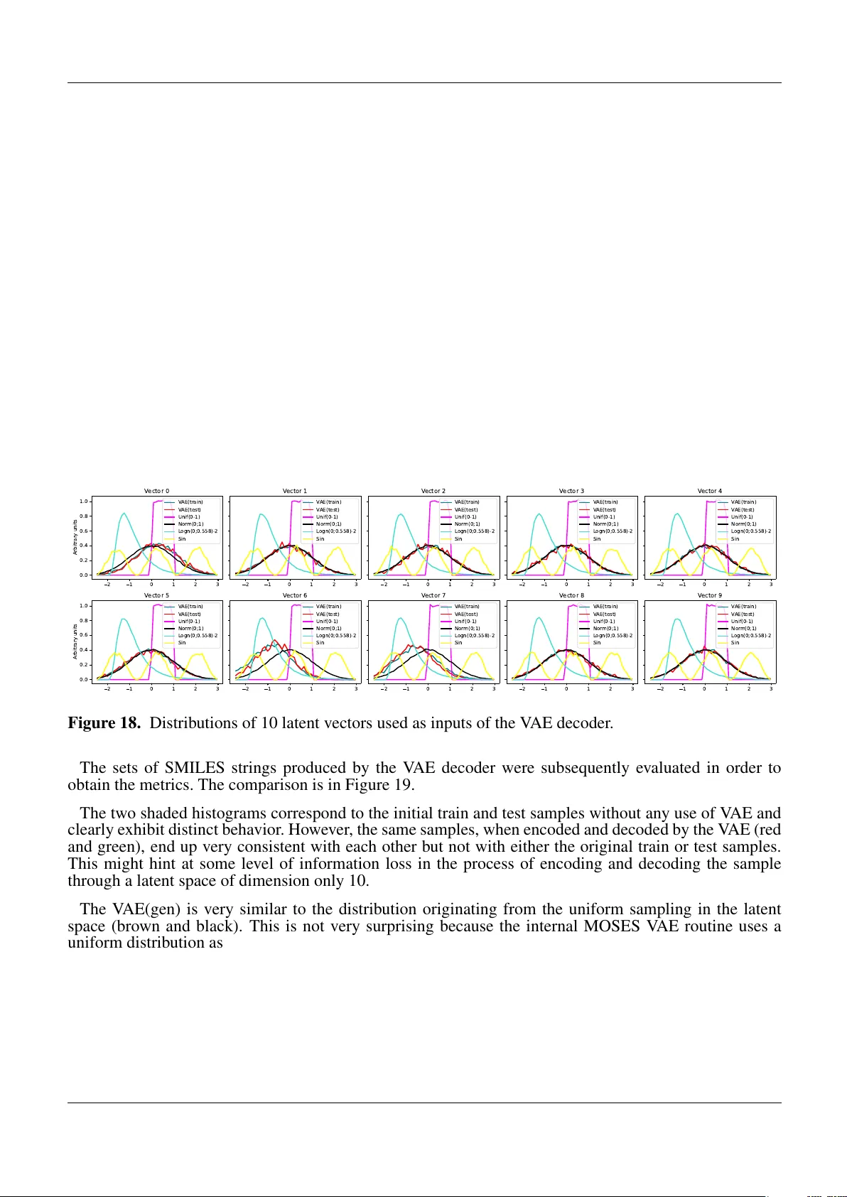
Latent Style-based Quantum W asser stein GAN f or Drug Design Julien Ba glio 1 , 2 , ∗ , Y acine Haddad 3 , 4 , ∗ and Richar d P olifka 2 1 Center f or Quantum Computing and Quantum Coherence (QC2), Depar tment of Ph ysics, Univ ersity of Basel, Klingelbergstr asse 82, CH-4056 Basel, Switzerland 2 QuantumBasel, Schorenweg 44b , CH-4144 Ar lesheim, Switzerland 3 Laboratory for High Energy Ph ysics (LHEP), Ph ysics Institute , F aculty of Sciences, Univ ersity of Bern, Sidlerstrasse 5, CH-3012 Ber n, Switz erland 4 Open Quantum Institute and Quantum T echnology Initiativ e, CERN, Esplanade des P ar ticules 1, CH-1211 Gene v a 23, Switz erland Correspondence*: julien.baglio@unibas.ch yacine .haddad@unibe .ch ABSTRA CT The de v elopment of ne w drugs is a tedious, time-consuming, and e xpensiv e process, f or which the av er age costs are estimated to be up to around $2.5 billion. The ﬁrst step in this long process is the design of the ne w drug, f or which de no v o drug design, assisted b y ar tiﬁcial intelligence, has blossomed in recent y ears and re v olutioniz ed the ﬁeld. In par ticular , gener ativ e ar tiﬁcial intelligence has deliv ered promising results in dr ug discov er y and de v elopment, reducing costs and the time to solution. Ho we v er , classical generative models, such as generativ e adversarial networks (GANs), are difﬁcult to train due to barren plateaus and prone to mode collapse . Quantum computing may be an a v enue to ov ercome these issues and provide models with f e wer parameters , thereby enhancing the generalizability of GANs. W e propose a ne w style- based quantum GAN (QGAN) architecture for drug design that implements noise encoding at e v er y rotational gate of the circuit and a g radient penalty in the loss function to mitigate mode collapse. Our pipeline emplo ys a v ariational autoencoder to represent the molecular str ucture in a latent space, which is then used as input to our QGAN. Our baseline model r uns on up to 15 qubits to validate our architecture on quantum simulators, and a 156-qubit IBM Heron quantum computer in the ﬁv e-qubit setup is used f or inf erence to inv estigate the effects of using real quantum hardw are on the analysis. We benchmark our results against classical models as provided b y the MOSES benchmark suite. Keyw or ds: drug design, smiles, ar tiﬁcial intelligence, latent space, variational auto-encoder , quantum machine learning, quantum generative adversarial netw orks, superconducting-qubit quantum computer 1 INTR ODUCTION The dev elopment of new pharmaceutical drugs is a lengthy , tedious, and expansi ve process. It takes usually 15 years, and the lower estimate of mean e xpense is around $1.3 billion 1–4 , and can rise up to around $2.5 billion 5,6 . The dev elopment cycle consists of the following main stages: target discov ery , molecular design, preclinical studies, clinical trials, and ﬁnally the regulatory approval to enter the market. In the ﬁrst two stages, there exist tw o ke y strategies for identifying viable drug candidates: either by modifying already existing commercial drugs, for e xample by performing a virtual screening, or by identifying new relationships between already known molecular structures and the desired activity; or by generating entirely new molecules, also called de-nov o drug design. In both methods there are multiple challenges, such as the safety of the candidate molecule, the efﬁcienc y , and ev entually the ability to manufacture the drug candidate. In this context, the emergence of artiﬁcial intelligence (AI) has re v olutionized the drug design approach, in particular the advances of generativ e AI which has been used for computer -assisted drug design in the past decade 7–9 . Generati ve Adv ersarial Networks (GAN) 10 are prominent AI models applied for drug design 11,12 . A GAN is composed of tw o neural networks: 1) a generator , which is trained to create ne w molecular structures from random noise input distribution; 2) a discriminator , which is trained to classify between the generator (fake) output, and the (real) molecular structures contained in the train input dataset. 1 Baglio et al. Latent Style-based Quantum WGAN for Drug Design The training scheme is an adversarial game, where the generator aims to fool the discriminator as much as possible while the discriminator aims to distinguish between real data and newly generated fake data, which in turn will help the generator to perform better . While GANs (and more generally AI models for drug design) ha v e blossomed in the past decade, their training can be computationally expensi ve when their scale is v ery lar ge, and the associated massi ve parameter space requires careful optimization 11 . GANs can suf fer from a non con ver gence of the adversarial training procedure, mode collapse when the generator only generates a sub-sample of the entire div ersity of the molecules present in the training set, or falling into a non-robust training pattern with a great sensiti vity to the hyperparameters of the models and to the initialization of the model weights. Quantum machine learning aims to provide new a venues to ov ercome some of these challenges. Quantum generativ e models 13–17 are generativ e models relying on the rules of quantum mechanics: Starting from quantum states encoding the problem, subject to the rules of superposition and entanglement, they build up the ﬁnal probabilistic output distribution using quantum measurements. Using spectral analysis, it has been shown that quantum neural netw orks probe different frequency modes compared to their classical counterparts, a feature which seems to be linked to higher expressi vity of quantum machine learning 18–21 . Quantum GANs (QGANs) 22–27 thus offer ne w av enues for po werful generati ve neural networks and ha v e been applied to drug design 28–31 . In 30,31 the authors hav e adopted the W asserstein distance as the backbone of the loss function (WGAN) 32 , leading to an improvement ov er the early QGAN in v estigations for drug discovery 28,29 . In 31 this was also supplemented by gradient penalty (WGAN-GP) 33 to impro ve trainability . In 30,31 the quantum architecture w as a modiﬁcation of the MolGAN architecture 34 , the standard in computer-assisted drug design, and the two studies applied their quantum models on dataset of small molecules, QM9 dataset 35 and PC9 dataset 36 . In this work we propose two improv ements: 1) going beyond small-molecule generation and 2) in v estigating sev eral modiﬁcations ov er the pre vious QGAN studies which enable a new state of the art for QGAN in computer-assisted drug design. First, we use the MOSES dataset and benchmark suite 37 , which is an industry-rele v ant dataset of SMILES molecules 38 not restricted to small molecules. In addition, aiming to exploit potential quantum advantages for sampling efﬁcienc y and model expressi veness and to address the challenge of mode collapse, we introduce a latent space approach in the quantum computing pipeline, follo wing classical GAN studies for drug design 39 . The input SMILES molecules of the training dataset are projected into an abstract vector space on which the training is done, before decoding the output back to the practical, physical space. Our last impro vement ov er previous quantum studies is the combination of this latent-space approach with a hybrid style-based quantum GAN 40,41 which uses data re-uploading, where the input noise distribution for the generator is inserted in all layers and not only in the ﬁrst initial layer of the neural netw ork. The style architecture was introduced for classical GAN in the context of image generation 42 and the latent style-based QGAN using WGAN-GP has been successfully tested for image generation 43 but nev er in v estigated for drug design. It should also be noted that the barren plateaus, where v anishing gradients render the training exponentially harder in the exploration of the loss function landscape, are less problematic when using the latent style-based approach for QGAN 43 . In addition, a recent study hinted to wards a potential quantum exponential adv antage with style-based QGAN in the number of trainable parameters 44 : an e xponentially smaller number of trainable parameters for QGANs compared to their classical counterpart, a feature which is of high interest for a complex computer-assisted drug design pipeline. The molecular structure is encoded following the SMILES approach. The SMILES strings are embedded into vectors of real numbers which are fed into the autoencoder projecting these vectors into an abstract latent vector space. The discriminator remains classical and we only use a parametrized quantum circuit for the generator . W e benchmark our new quantum drug design architecture against classical latent GAN approach based on the widely used MOSES benchmark suite and show that our proposed latent style-based QGAN can be very efﬁcient for drug design with far fe wer trainable parameters than their classical counterparts. Our pipeline uses RDKit 45 to check that the ne w generated molecular structures from our pipeline do correspond to v alid (bio)chemical compounds and to calculate relev ant metrics. The training of our quantum computing pipeline is performed on noiseless quantum simulator , including the sampling of 30,000 new molecules to v alidate the pipeline. W e also perform the sampling of 2,500 2 Baglio et al. Latent Style-based Quantum WGAN for Drug Design ne w , viable molecular structures on ibm_kingston, a 156-qubit IBM Heron quantum computer , using the model trained on quantum simulator . Using MOSES benchmark suite, we also quantify the quality of our output with metrics such as internal di v ersity , molecular weight, LogP , or quantitati v e estimation of drug-likeliness. Our proposed quantum pipeline, tested on a real-w orld dataset not restricted to small molecules, greatly enhances the explainability of computer-assisted drug design by using far less trainable parameters than con v entional classical AI pipeline for drug discov ery . The statistical overall score of our pipeline demonstrates that it is competitiv e with classical AI pipeline, with ev en statistically signiﬁcant improv ements ov er classical GANs for some of the indi vidual metrics we ha ve in vestigated. 2 MA TERIALS AND METHODS 2.1 Dataset construction W e use the MOSES dataset 37 as our main analysis dataset. This dataset is built out of the ZINC Clean Leads collection 46 and contains ov er 1.9M molecules of interest for biochemistry applications. W e ha ve further applied a random sampling of the dataset to obtain 12,000 molecules for training and 4,087 molecules for v alidation. The reason for this do wnsize of the original MOSES dataset is two-fold: 1) we can test the small- dataset regime and show the capabilities of quantum-computing-assisted pipeline to perform well on small datasets; 2) in the proof-of-concept phase of our new quantum architecture, it helps to v alidate the concept within a short runtime. The MOSES dataset is a high-dimensional dataset which is currently not practical to be used directly on a quantum computer , due to limited av ailability of resources of current quantum hardware. W e thus pre-process the data by transforming the SMILES strings into high-dimensional molecular descriptors using RDKit features 45 , which will be used for calculating the various metrics. The SMILES strings are then fed to an auto-encoder , see belo w , to compress the (high-dimensional) molecular alphabet into a latent representation (low-dimensional features), which is in turn compact enough to be used for the quantum part of our pipeline. The decoder part of the auto-encoder allo ws to map the generated latent features back into valid SMILES molecules. In order to check the chemical properties of the both the randomly selected samples for our ﬁnal training and testing dataset as well as the generated samples, we hav e used RDKit ﬁlters 45 . Our procedure balances chemical validity , through the auto-encoder and the RDKit validation, with quantum feasibility allo wed by the low-dimensional latent-feature encoding. When generating ne w molecules, we have sampled 30,000 molecules unless stated otherwise, follo wing the default v alue used in the MOSES benchmark suite. 2.2 Description of the pipeline The structure of the molecules contained in our dataset is encoded using SMILES strings 38 . A standard method in classical generati ve approach for drug design uses a pre-trained auto-encoder to project the SMILES strings into a compact latent space, which is much more tractable that the original strings for the generativ e models. Note that the v ery ﬁrst step before the auto-encoder is the extraction of chemical features from the SMILES strings using RDKit 45 in order to get the relev ant metrics. The auto-encoder captures salient chemical features while reducing dimensionality , allowing to operate in a manageable latent representation. Follo wing this approach also used in the MOSES benchmark suite, our pipeline starts with a pre-trained V ariational Auto-Encoder (V AE) to encode the drug-like SMILES molecules into the latent space. T o perform the generation of new molecules we use a Generativ e Adversarial Netw ork (GAN) 10 . A GAN is composed of two netw orks competing against each other: a generator , sampling new candidates from a random number input distribution; and a discriminator , acting as a binary classiﬁer trained to distinguish between real input data and generated samples from the generator . The training is an adversarial procedure, a two-player minmax game between the two networks, until ideally a Nash equilibrium is reached, when the generator has become so good that the discriminator cannot distinguish anymore between real input data and generated samples. W e will compare the classical GAN implementation as provided in the MOSES benchmark suite against our proposed quantum GAN architecture. 3 Baglio et al. Latent Style-based Quantum WGAN for Drug Design Quantum computing is a different paradigm to perform computations. Instead of the classical bits which hav e binary outcomes (0 or 1), quantum computers use qubits (quantum bits) which are quantum states of a controlled two-lev el quantum system. Follo wing the laws of quantum mechanics, the qubits are subject to superposition and entanglement, which in turn means that they li v e in a much more complex space than traditional bits and are not restricted to binary outputs, allo wing for a more di verse exploration of the solution space for generativ e modelling applications. A class of such quantum algorithms is parameterized quantum circuits (PQC) 47 , where the qubits are subjected to quantum operations (gates) which are parameterized by real numbers (rotation angles) and arranged in a circuit of consecutiv e operations. The ﬁnal quantum state is then measured and the output measurement are collected and statistically create the ﬁnal outcome. A classical training procedure allows to optimize these rotation angles which the trainable parameters of the quantum network formed by this PQC. In our pipeline the generator will be a quantum network that will be trained on an ideal (noiseless) quantum simulator while the discriminator remains a classical network. The generator outputs are latent v ectors in the same latent space as the V AE. T o obtain the ﬁnal generated molecules the generator output is fed back to the decoder part of the V AE. Our analysis consists of the follo wing steps: 1. T rain the V AE and optimize the V AE hyperparameters; 2. Use the encoder part of the V AE to transform the input dataset into input latent vectors, train the GAN with these input latent vectors; 3. Optimize the latent classical GAN hyperparameters relev ant for the discriminator; the classical generator is already optimized and follo ws the MOSES benchmark suite; 4. Replace the classical generator by a quantum generator , train and optimize; 5. Use the decoder and an RDKit validation to produce ﬁnal generated molecule samples; Perform a comparison between classical and quantum GAN performances with a set of metrics (see belo w), perform inference on a real quantum hardware. W e present a compact representation of the proposed drug-design pipeline in Figure 1. In our benchmark against classical drug-design pipeline, the quantum generator depicted in red is replaced by a classical generator with a structure follo wing that of the latent GAN from the MOSES benchmark suite. W e hav e used Torch v2.8.0 48 and Pennylane v0.42.3 49 to implement our pipeline ran on an NVIDIA A100 GPU with 40GB of memory . 2.2.1 V AE and latent dimension The architecture of the V AE, taken over from the MOSES benchmark suite together with default parameter settings, uses Gated Recurrent Units (GR Us) as b uilding blocks. The encoder is made of one bidirectional GR U ( n l = 1 ) with a hidden dimension D h = 256 , follo wed by tw o linear output layers transforming the output vector of the GR U to a vector of the latent space. The decoder is made of three layers of GR U ( n l = 3 ) with hidden dimensions D h = 512 , each layer (e xcept the last one) follo wed by a dropout layer . The default dropout probability out of MOSES benchmark suite is zero (hence no dropout layer in practice), but we will later e xplore the impact of non-zero dropout probabilities. The SMILES string is tokenized, such that each character of the string is associated to an integer ID, which in turn is embedded as a vector (initially a one-hot v ector , b ut the embedding is also part of the training of the V AE to increase efﬁcienc y) according to the SMILES vocab ulary table, the dimension of that vector corresponding to the number of characters in the v ocab ulary table. As such, the GR U processes the input as a sequential data x t where each element of the sequence is a vector representing the embedded token ID. The v ariable t index es the character ID positioning in the SMILES string from left to right, equiv alent to a temporal index. At a gi ven step t , a GR U uses two gates to update the internal hidden state h t : the reset gate r t and the update gate z t . The hidden state h t is thus computed from the 4 Baglio et al. Latent Style-based Quantum WGAN for Drug Design Figure 1. Schematic representation of the quantum-augmented drug-design pipeline. The model comprises a pre-trained V AE on the MOSES dataset using SMILES input (in purple), that embeds the original molecules into a lo w-dimensional latent space, and a quantum GAN with a quantum generator (in red) and a classical discriminator (in blue). The features extracted by the V AE from the input dataset are used for the training of the GAN. The ﬁnal generated SMILES molecules are reconstructed by in v ersely transforming the features generated by the quantum generator using the pre-trained decoder of the V AE, and ﬁnally v alidated using RDKit. hidden state h t − 1 and the ne w candidate hidden state n t as follo ws: r t = σ ( W r x t + U r h t − 1 + b r ) , z t = σ ( W z x t + U z h t − 1 + b z ) , n t = tanh  W n x t + b n + r t ⊙ ( U n h t − 1 + b n,u )  , h t = (1 − z t ) ⊙ n t + z t ⊙ h t − 1 , (1) where the function σ is the sigmoid function controlling the gating mechanism and ⊙ stands for Hadamard product (or element-wise product). As a slight abuse of notations, both tanh and σ functions are meant to be applied element-wise on each element of the vector ar gument of these functions. The matrices W r /t/n and U r /t/n are the input trainable weights and recurrent trainable weights for the reset gate, the update gate, and the candidate hidden state, respecti vely . The vectors b r /z/n and b n,u are the associated trainable biases for each gate. Note that for the ﬁrst letter (equi v alent to t = 0 ) h t − 1 corresponds to the initial hidden state at time t = 0 . For a bidirectional GR U, the sequence ( x t ) is processed in both forward and backward directions, producing a ﬁnal state which has doubled dimension, h bi GRU = ( h → , h ← ) . At each step the output is a concatenation of the forward direction (processing the SMILES string from left to right) and the backw ard direction (processing the SMILES string for right to left). It is important for the encoder of the V AE as it captures information from both past and future contexts in the SMILES string, in turn allowing for a richer and more accurate encoding of the SMILES sequence. When there are more than one layer in the GR U, the input of layer l is the ﬁnal hidden state (output) of layer ( l − 1) , h ( l − 1) t . When a dropout layer is 5 Baglio et al. Latent Style-based Quantum WGAN for Drug Design included, the actual input of layer l is a modiﬁcation of h ( l − 1) t into δ ( l − 1) t h ( l − 1) t where δ ( l − 1) t is a Bernoulli random v ariable equal to zero with a probability equal to dropout. The dimensionality of the latent space is a key parameter of the pipeline. The output of the generator , both for the classical and quantum GANs, has to match the dimension of the latent space. For the quantum generator there is a linear correspondence between the number of qubits used in the quantum circuit and the latent dimension D l : either a one-to-one correspondence or a one-to-two, depending on how the measurements outcome from the quantum network is collected, see the ne xt sections. As current quantum computers are still limited in the number of qubits, and as the simulation of quantum states with classical resources is e xponentially costly , our default setup for latent space is a latent dimension of 10, hence using at most 10 qubits. W e hav e studied a latent dimension up to 30 and validated our pipeline by performing the training on noiseless quantum simulators using classical resources. W e ha v e also performed an inference on a superconducting-qubit hardware, theibm_kingston computer with 156 qubits on an IBM Heron chip. 2.2.2 Classical and h ybrid quantum GAN architecture The heart of our pipeline is the GAN architecture. Let us deﬁne the generator as G and the discriminator as D . The training of the adversarial minmax game of the GAN uses the Earth-Mov er (or W asserstein) distance, together with gradient penalty (WGAN-GP), to ensure an ef ﬁcient mitigation of the ef fect of mode collapse 33 . The training of the WGAN-GP follo ws from min G max D L W GAN ( G, D ) + λ E ˆ x ∼ p ( ˆ x ) h ( ||∇ ˆ x D ( ˆ x ) || 2 − 1) 2 i , (2) where ˆ x are samples drawn randomly from a uniform distribution p ( ˆ x ) , along straight lines between pairs of points sampled from the input data distrib ution and the distrib ution of the generated output from the generator G . W e denote the input data distrib ution as p data and p ( ξ ) the noise distrib ution which serves as input for the generator G . The function L W GAN ( G, D ) is the loss function of the original W asserstein GAN without the gradient penalty , and corresponds to L W GAN ( G, D ) = E ξ ∼ p ( ξ )  D ( x = G ( ξ ))  − E x ∼ p data  D ( x )  . (3) The parameter λ controls the impact of the gradient penalty term and is ﬁxed to λ = 10 33 . A WGAN-GP can still suffer from training instability , difﬁculties for generalization, or a lack of robustness, which is reﬂected by a sensitivity to the initialization of the trainable parameters of the GAN. Our pipeline hence replaces the WGAN-GP by a hybrid quantum WGAN-GP (from now on simply classical GAN and QGAN), where the discriminator is still a classical network b ut the generator is no w a quantum generator described by a PQC. Follo wing pre vious studies in the context of high-ener gy physics or high-quality image generation 40,41,43 we adopt a style-based architecture 42 in the quantum generator 40 . It uses a data re-uploading approach where the input random noise for the generator is implemented in all gates of the quantum circuit, and not just in the ﬁrst gates on each qubit. This approach has been sho wn to allo w for more ﬂe xibility and richness of the quantum generation mechanism for images or high-ener gy physics applications, b ut has ne ver been attempted for drug design so f ar . The classical GAN architecture in our benchmark follo ws closely the one from MOSES benchmark suite 37 introduced in 39 . The discriminator (same structure for classical and quantum GANs) is made of three linear (dense) layers for which the dimension of each layer follo ws the sequence [512 , 256 , 1] , all follo wed by a LeakyReLU activ ation function with parameter 0.2, except for the last layer . The classical generator is mode of ﬁ v e linear layers with the sequence [128 , 256 , 512 , 1024 , D l ] , each followed by a LeakyReLU activ ation function with parameter 0.2, except for the last layer . In addition, the second, third, and fourth layer use batch normalization. W e will study two different ansätze for the quantum circuit of the quantum generator that are built from layers which can be repeated n l times to increase the expressi ve power of the model. Such layered structures follo w the hardw are-ef ﬁcient ansätze paradigm widely used in v ariational quantum algorithms, including the v ariational quantum eigensolver and v arious QGAN studies 25,47,50,51 . In particular , the 6 Baglio et al. Latent Style-based Quantum WGAN for Drug Design AAAEwHicrVNNb9NAEN0YA8VQaODIxSICcYpst3G5IJVERD2AVFDTVoqjaG1P3FXWa3d33ZKs/Ed6hT/Fv8FxkzRfFRJ0JEtv5r19M/as/ZQSIS3rd0V7oD989HjrifH02fbzFzvVlyciyXgAnSChCT/zsQBKGHQkkRTOUg449imc+sPWhD+9BC5Iwo7lKIVejCNGBiTAsij1q9q250NEmLrIMJNkOM7NLk+uTAHpR6vuBHHPeGd6EZagvvdHuXmbjBeTDUwgOVX2BM5jCRYS71+9JeaRys072/yH94LL5jb34/3XNvfc5I5+nuEBC2+X39+pWXWrDHMd2FNQQ9M46lcr116YBFkMTAYUC9G1rVT2FOaSBBRyw8uKq4SDIY6gW0CGYxA9VV7c3HxbVEJzkPDiYdIsq4snFI6FGMV+oYyxPBer3KS4ietmcvChpwhLMwksWJpClS9aViaIEp9jPpp/Amd55PCSpGI69I+bqQ3DC2FQ/G9lqjiEuTo8/volV22n0W608mXepxnMBM7efvOTtSIYAaXJ1dyj/dly3TWPYpyZYq/dsBr2iiLiAGymcNstu7mbG8U27dXdrYMTp267dfebUztoTve6hV6jN+g9stE+OkCH6Ah1UKBJ7Vr7qf3Sm/q5nugXN1KtMj3zCi2FPv4DRdBzcg== R y R z R y R z R y R z R y R z R y R z R y R z R y R z R y R z R y R z R y R z Figure 2. Styled simple circuit with ﬁv e qubits and one layer . AAAGIHicrZTPb9MwFMfdtYERfq1w5BJRgThVSVg7LkijFVUPIA20bpOaqnKS12LVcYLtbBQr/whH/hpuCIkL/CmcSLN2tBmLWsSTIr0f3/fysS3bjSgR0jR/lLbKFe3a9e0b+s1bt+/c3aneOxJhzD3oeSEN+YmLBVDCoCeJpHASccCBS+HYnbRn9eNT4IKE7FBOIxgEeMzIiHhYpqlhtRw4LowJU+9jzCSZfEyMPg/PDAHRc7Nue8FAf2w4YyxBdRNj4b4dTpeDtGkWeZJTZaX+LFq2gujqiYuB9hoDHWcDypBJHlK1CXMRZU5XwLwBZX7oWszFe7k8ooj5nynXZN5kLwuY/w/llT9cn7Jw2Y7uAPP/XK7hTs2sm5kZlx1r7tTQ3A6G1dInxw+9OAAmPYqF6FtmJAcKc0k8ConuxOlVxd4Ej6GfugwHIAYqexgS41Ga8Y1RyNOPSSPLLncoHAgxDdxUGWD5TuRrs+Tfav1Yjp4NFGFRLIF5KxQqW2iWmXmUuBzz6cUW2KvI/imJxBz6wzm1rjs+jNL3LAsVBz9R3cPXrxLVsRudRjtZrbs0hoXA3t1rvTBzgilQGp5dzOi8NJvNSzNSnIVit9MwG1ZOMeYAbKFodtpW62mip6dp5c/usnNk161mvfnGru235ue6jR6gh+gJstAe2kdddIB6yCt/L/+qlCsV7bP2RfuqfTuXbpXmPffRimk/fwMpL8Cj H R y R z R y R z H R y R z R y R z H R y R z R y R z H R y R z R y R z H R y R z R y R z Figure 3. Styled basic entangled layer (BEL) circuit with ﬁv e qubits and one layer . In addition there is a ﬁnal set of one-qubit R Y gates on each qubit to rotate all qubits in the computational basis before performing the ﬁnal measurement operation. designs are inspired by parameterized circuit templates a v ailable in modern quantum machine-learning frame works such as PennyLane 49 . The ﬁrst architecture corresponds to a simple structure composed of single-qubit rotations and controlled rotations arranged in repeated layers (Fig. 2), while the second architecture introduces a basic entangled layer (BEL) (Fig. 3) that enhances correlations between qubits through additional entangling operations 52 . W e consider representati ve circuits with ﬁv e data qubits. All rotation gates, including the controlled rotation gates, are parameterized by angles in the domain [0 , 2 π ] , deﬁned as θ q ,ℓ,k = 2 π tanh  ξ q W q ℓk + b q ℓk  , (4) where ξ q is the input noise vector element for a gi v en qubit q , W q ℓk is the element of the tensor of trainable parameters, for a gi ven qubit q , a gi v en layer l , and a gi ven angle label k corresponding to the k th rotation gate. The tensor b contains the biases. Using the non-linear function tanh() helps to av oid ov er -rotation during the training phase, further mitigating the (quantum) mode collapse. W e construct output vectors from the quantum circuit by performing quantum measurements of Pauli operators, constructing an expectation v alue of it. W e can use either single readout or dual readout. In the former case one Pauli operator (usually chosen as the Z operator) is measured for each qubit, so that a quantum generator with n q b qubits produces a latent vector of dimension n q b . In the latter case, the dual readout, we exploit the non-commutativity of Pauli X and Pauli Z operators to use the same quantum circuit b ut performing tw o independent measurements for each qubit. The quantum generator with n q b qubits thus outputs a latent vector of dimension 2 n q b , at the expanse of running twice as many quantum measurements to obtain the same similar quantum precision of the ﬁnal outcome compared to single readout. Because of the e xponential cost of simulating quantum circuits, we hav e restricted ourselves to up to 15 qubits with dual readout in our analysis, corresponding to a maximum latent dimension of 30. W e have adopted the latent dimension of 10 as our default setting, with either 10 qubits and single readout or ﬁ ve qubits and dual readout, as used for the quantum inference on ibm_kingston. This choice of default latent dimension is driv en by the analysis of the classical latent GAN, where a latent dimension greater than 10 does not change signiﬁcantly the results, see also T able 20 in the supplementary material section. W e will also present results on quantum simulator with a latent dimension of 30, with 15 qubits and dual readout. 7 Baglio et al. Latent Style-based Quantum WGAN for Drug Design 2.3 Metrics The deﬁnitions of the metrics used in this analysis are taken from the MOSES benchmark suite and are standard for drug design. W e list them below: • Distinct Fraction ( ϵ d ) : Calculates fraction of molecules after string de-duplication has been applied to the generated SMILES molecules. • Fraction of valid molecules ( ϵ v ) : Reports the v alidity of generated SMILES strings and is deﬁned using RDKit molecular structure parser that checks atom valenc y and consistency of bonds in aromatic rings. • Fraction of unique molecules ( ϵ u ) : Checks that the model does not collapse to producing only a fe w typical molecules. • Novelty : Fraction of the generated molecules that are not present in the training set. Low no velty indicates ov erﬁtting. • Filters : is the fraction of generated molecules that pass ﬁlters applied during dataset construction. While the generated molecules are often chemically valid, they may contain unwanted fragments that were remov ed from the training set. • Internal diversity (IntDiv) : Assesses the chemical div ersity within the generated set of molecules. This metric detects a common failure case of generativ e models—mode collapse. W ith mode collapse, the model produces a limited set of samples, ignoring some regions of chemical space. • Molecular weight (W eight) : Sum of atomic weights in a molecule. In general, it is easier to build viable drugs from lighter molecules. • LogP : Octanol-water partition coefﬁcient, a ratio of a chemical concentration in the octanol phase to its concentration in the aqueous phase of a two-phase octanol/water system. It is a measure of lipophilicity and is deﬁned as the ability of a compound to differentially dissolve in a mixture of water and lipids/organic solv ents. Using MOSES tools it is computed with the RDKit Crippen estimator 53 . According to the Lipinski’ s rule of 5 54,55 , a typical good value of LogP for (oral) drugs is between 0 and 5. W e hav e constructed an associated metrics, ϵ Log P , which is the fraction of molecules in this range. • Synthetic Accessibility Score (SA) : Heuristic estimate of how hard (10) or how easy (1) it is to synthesize a gi ven molecule. • Quantitative Estimation of Drug-likeness (QED) : Real number in the interval [0; 1] , estimating ho w likely a molecule is a viable candidate for a drug. The ﬁrst six metrics are constrained to the interv al [0; 1] , where the desired value is as close to unity as possible. The last four metrics are reported in two ways: either as the W asserstein distance (denoted as W ) between the test and generated dataset, follo wing the MOSES benchmark suite 37 ; or as the mean of the distribution itself, calculated on the generated sample. The latter choice allows for removing an y dependency of the results on the test dataset and is the preferred choice in our analysis. As mentioned in the list above, we have also introduced another metric not present in the MOSES analysis 37 , the fraction ϵ Log P . As the MOSES analysis was not necessarily restricted to (human) drug discov ery , this new metric helps to quantify how many drug candidates we obtain in our quantum- computer-assisted drug-design pipeline are compatible with typical LogP values encountered in viable drugs. It is important to av oid a chemical compound with too high lipophilicity (which can lead to accumulation in f at tissues and fatal toxic issues, or dif ﬁculties to penetrate certain barriers in the body) or too low lipophilicity (the compound cannot bind to the target molecule at all). Small negati v e v alues for LogP are typical of drug that can be injected, v alues between 1.3 and 1.8 are ideal oral candidates, values around 2 are good candidates for targeting the central neural system, for e xample. There are three dif ferent scenarios where the abov e-mentioned metrics ha ve been used: 1. V AE hyperparameter optimization: The aim is to ensure a good ability to encode/decode the SMILES information into/from the latent dimension. W e thus aim to maximize internal di versity . Additionally , to suppress ov er -training and improv e generalization, we aim to minimize W ( LogP ) , W ( W eight ) , W ( SA ) , and W ( QED ) . 8 Baglio et al. Latent Style-based Quantum WGAN for Drug Design 2. GAN hyperparameter optimization: The aim is to improve stability of the training. For the scope of this analysis, only the ratio of training frequency between the generator and discriminator within a gi ven epoch has been changed. 3. Classical and quantum GAN performance comparison: The aim is to compare performance independently of the training or test samples as well as to maximize the chance for generating truly nov el molecules. Therefore, all fractions ( ϵ d , ϵ v , ϵ u , ϵ Log P , novelty , ﬁlters, and internal div ersity) hav e been maximized as well as the mean of the QED distrib ution, while the means of the SA and molecular weight distributions ha v e been minimized. In order to test the training rob ustness (i.e. the sensitivity of the model to the initialization of the training parameters), each model has been trained ﬁv e times with each time a different random seed, so that the quoted v alues are the mean and standard de viation ov er these ﬁ ve runs. In order to assess globally the performance of the quantum GAN models against the classical GAN, we hav e also used as a ﬁnal metric the Z 0 signiﬁcance deﬁned as: Z 0 = X m Z m 0 = X m ∆ m p ( σ m 1 ) 2 + ( σ m 2 ) 2 , (5) where the sum runs over all the relev ant metrics for scenario comparison as listed in the list above (fractions ϵ d , ϵ v , ϵ u , ϵ Log P ; nov elty; ﬁlters; internal di versity; ⟨ QED ⟩ ; ⟨ SA ⟩ ; ⟨ W eight ⟩ ) and ∆ is the dif ference between the means of the respecti v e metric m . The quantities σ m 1 and σ m 2 in Equation 5 refer to the standard deviations of the metric m for the reference scenario and for the scenario under study , respecti vely . The construction ∆ depends of whether the metric m is aimed to be maximized or minimized. In the former case, such as for ef ﬁciencies, ∆ m = µ m 2 − µ m 1 where µ m 1 and µ m 2 refer to the means of the metric m for the reference scenario and for the scenario under study , respecti v ely . In the later case, such as for the SA or W eight, µ m 1 and µ m 2 are swapped, ∆ m = µ m 1 − µ m 2 . For global signiﬁcance, we will take the a v erage of Z 0 , hence di viding by the number of metrics used in the comparison. The ground truth in this calculation is the classical GAN result taken as the benchmark reference point. The sign of the signiﬁcance then indicates impro vement or degradation of the quantum GAN designs over the classical GAN. T o guide the reader , we remind |⟨ Z 0 ⟩| < 1 indicates globally a performance which is comparable between classical and quantum pipelines (the variance is less than 1 σ ), while values above indicate sizable improv ement or sizable degradation. More details with an e xample are presented in Section 2.4.2. W e present in the supplementary material more details on the metrics applied to the input distributions, see Section 1 of the supplementary material. For more details on the sensitivity of the metrics to the number of generated samples, see Section 3. 2.4 T raining details 2.4.1 T raining of the V AE The V AE has been trained following the procedure in the MOSES benchmark suite 37 . This means in particular that we have used a batch size of 64 and a gradient clipping threshold of 50. W e have used Adam optimizer 56 with a nominal learning rate equal to 3 × 10 − 4 . The study of the loss function for training and v alidation datasets has indicated that N ep = 1 , 000 epochs produce an optimal result. W e ha ve performed a small hyperparameter tuning of the V AE by varying the parameters listed in T able 1. The learning rate is ﬁx ed at 3 × 10 − 4 in the nominal setup, we explore also a learning-rate scheduling for which the tuned parameter is a cosine schedule starting from 10 − 3 and ending at 10 − 5 for the ﬁnal training epochs. W e pro vide the tuned v alues of these parameters, leading to the metrics comparison presented in T able 2. The comparison of the v arious metrics distributions between the nominal and the tuned V AE is presented in Figure 4. W e provide more details on the V AE training results in the supplementary material, Section 2 of the supplementary material. Overall, the performance of all V AE training runs is v ery good and consistent: The metric comparison sho ws an impro v ement for the tuned V AE, ho we v er modest. W e ha ve also performed an additional test of the robustness of the decoder of the V AE, to ensure that it can ef ﬁciently decode the latent space since this is how we obtain the ﬁnal generated molecules. This means we have to mak e sure that the decoder does 9 Baglio et al. Latent Style-based Quantum WGAN for Drug Design Metrics Nominal V AE T uned V AE Learning rate (lr) 3 × 10 − 4 Scheduled 10 − 3 → 10 − 5 Encoder n l 1 1 Encoder D h 256 512 Decoder n l 3 4 Decoder D h 512 512 Decoder dropout 0 0.75 T able 1. V AE hyperparameter settings comparison between nominal (MOSES default) and tuned settings. Metrics T rain set Nominal V AE T uned V AE IntDi v 0.898 0.896 0.896 W ( LogP ) 0.091 0.087 0.079 W ( SA ) 0.268 0.275 0.251 W ( QED ) 0.027 0.025 0.022 W ( W eight ) 42.8 43.9 41.8 N par ams – 4,271,250 6,472,082 T able 2. Metrics deri v ed from the training set and sets generated by the nominal and tuned V AE. Internal di versity is computed as the mean o ver the respecti v e samples, whereas the remaining four metrics are the av erage W asserstein distances between the sample in question and the test sample for the corresponding metric. 0.800 0.825 0.850 0.875 0.900 0.925 0.950 0.975 1.000 Inter nal diversity 0 5 10 15 20 Arbitrary units T rain N o m i n a l D l = 1 0 T u n e d D l = 1 0 T u n e d D l = 2 0 T u n e d D l = 3 0 4 2 0 2 4 6 8 10 12 L ogP 0.00 0.05 0.10 0.15 0.20 0.25 0.30 Arbitrary units T rain N o m i n a l D l = 1 0 T u n e d D l = 1 0 T u n e d D l = 2 0 T u n e d D l = 3 0 0 1 2 3 4 5 6 7 8 S A 0.0 0.1 0.2 0.3 0.4 0.5 Arbitrary units T rain N o m i n a l D l = 1 0 T u n e d D l = 1 0 T u n e d D l = 2 0 T u n e d D l = 3 0 0.0 0.2 0.4 0.6 0.8 1.0 Quantitative estimation of drug-lik edness 0.0 0.5 1.0 1.5 2.0 2.5 Arbitrary units T rain N o m i n a l D l = 1 0 T u n e d D l = 1 0 T u n e d D l = 2 0 T u n e d D l = 3 0 0 200 400 600 800 1000 W eight 0.000 0.001 0.002 0.003 0.004 0.005 Arbitrary units T rain N o m i n a l D l = 1 0 T u n e d D l = 1 0 T u n e d D l = 2 0 T u n e d D l = 3 0 Figure 4. Distrib utions of metrics deriv ed from the input train set and the generated sets using the nominal and tuned V AE decoder . not collapse the latent space back to a small subset of the molecular space. A shape study of the decoder has been performed and demonstrates that it is sensiti ve to the shape of the latent vector distribution, conﬁrming that the V AE does not collapse to a contriv ed subspace of the molecular input space. For more details, see Section 5 of the supplementary material. 10 Baglio et al. Latent Style-based Quantum WGAN for Drug Design 2.4.2 Latent GAN The latent QGAN is trained on a noiseless quantum simulator (state-vector simulation) and the ﬁnal generated molecules are ﬁltered with RDKIT to check that they are chemically valid. W e will also perform an experimental sampling on a quantum hardware, the IBM ibm_kingston system based on the Heron quantum chip. The training of both classical and quantum latent GANs follows from the loss function described in Equations 2 and 3 using again the Adam optimizer . F or the classical GAN, the nominal learning rate is 2 × 10 − 4 with Adam parameters β 1 = 0 . 5 and β 2 = 0 . 9 . The number of epochs has been set to N ep = 100 , and the ratio of the discriminator to generator training frequency was changed from ﬁ ve (default in MOSES benchmark suite) to one (further denoted as “tuned GAN”). The loss functions for the nominal and tuned GANs ov er a number of epochs are presented in Figure 5. 0 20 40 60 80 100 Epoch 1.5 1.0 0.5 0.0 0.5 1.0 L oss GAN T raining for our nominal model: L oss function as a function of the epoch Generator loss - T raining set Discriminator loss - T raining set 0 20 40 60 80 100 Epoch 1 0 1 2 3 4 L oss GAN T raining for our tuned model: L oss function as a function of the epoch Generator loss - T raining set Discriminator loss - T raining set Figure 5. Comparison of the loss functions for the nominal (left) and tuned (right) GANs. Each model was run with ﬁ v e dif ferent seeds, the shaded band denotes a ± 1 σ deviation. Metrics T rain set T uned V AE Nominal GAN T uned GAN ϵ d 0.982 0.605 ± 0.017 0.510 ± 0.007 0.481 ± 0.030 ϵ v 1.000 0.868 ± 0.006 0.911 ± 0.006 0.917 ± 0.012 ϵ u 1.000 0.993 ± 0.001 0.986 ± 0.002 0.986 ± 0.003 Nov elty 0.000 0.461 ± 0.026 0.501 ± 0.015 0.536 ± 0.015 Filters 0.734 0.728 ± 0.002 0.723 ± 0.003 0.721 ± 0.011 IntDi v 0.898 0.896 ± 0.000 0.902 ± 0.002 0.898 ± 0.004 W ( LogP ) 0.091 0.078 ± 0.004 0.291 ± 0.026 0.354 ± 0.037 W ( SA ) 0.268 0.249 ± 0.004 0.375 ± 0.028 0.437 ± 0.080 W ( QED ) 0.027 0.023 ± 0.001 0.039 ± 0.003 0.038 ± 0.005 W ( W eight ) 42.8 42.4 ± 1.0 93.0 ± 4.6 99.4 ± 10.6 ϵ Log P 0.883 0.886 ± 0.003 0.895 ± 0.002 0.898 ± 0.006 ⟨ SA ⟩ 2.561 2.579 ± 0.004 2.454 ± 0.028 2.391 ± 0.080 ⟨ QED ⟩ 0.596 0.604 ± 0.001 0.592 ± 0.006 0.599 ± 0.007 ⟨ W eight ⟩ 261.5 260.5 ± 1.1 210.3 ± 4.6 203.9 ± 10.6 ⟨ Z 0 ⟩ – Reference +1.45 +0.86 T able 3. Metrics results for the V AE and classical GANs. All GANs use the tuned V AE for the latent space representation. Unlike the other cases, the nominal GAN uses the nominal GAN hyperparameter settings as discussed in the text. The quoted standard deviation comes from running each scenario ﬁ ve times with dif ferent seeds for the initialization of the trainable parameters. 11 Baglio et al. Latent Style-based Quantum WGAN for Drug Design 0.800 0.825 0.850 0.875 0.900 0.925 0.950 0.975 1.000 Inter nal diversity 0 5 10 15 20 Arbitrary units T rain T est V AE Nominal GAN T uned GAN 4 2 0 2 4 6 8 10 12 L ogP 0.00 0.05 0.10 0.15 0.20 0.25 0.30 0.35 Arbitrary units T rain T est V AE Nominal GAN T uned GAN 0 1 2 3 4 5 6 7 8 S A 0.0 0.1 0.2 0.3 0.4 0.5 0.6 0.7 Arbitrary units T rain T est V AE Nominal GAN T uned GAN 0.0 0.2 0.4 0.6 0.8 1.0 Quantitative estimation of drug-lik edness 0.0 0.5 1.0 1.5 2.0 2.5 3.0 Arbitrary units T rain T est V AE Nominal GAN T uned GAN 0 200 400 600 800 1000 W eight 0.000 0.001 0.002 0.003 0.004 0.005 0.006 0.007 0.008 Arbitrary units T rain T est V AE Nominal GAN T uned GAN Figure 6. Comparison of the metrics for the models used in the analysis. For the V AE, the tuned version is used, for the GAN, not only the tuned V AE is used but also the GAN is tuned itself. Each model was run with ﬁ ve dif ferent seeds, the shaded band is deﬁned as ± 1 σ deviation. W e present in T able 3 the metrics estimated from the samples generated by the respecti ve models. The table is split into four parts: 1. The ﬁrst six metrics are interpretable as efﬁciencies – distributions between 0 and 1 estimated from the distributions themselv es, where the closer to unity , the better . 2. The second part, denoted with W ( X ) , presents the W asserstein distances between the test sample and the generated sample for a v ariable X deﬁned by the MOSES analysis. 3. The third part presents the fraction of the samples with | Log P | < 5 and mean v alues of the distributions of the Synthetic Accessibility Score (SA), Quantitati ve Estimation of Drug-likeness (QED), and molecular weight. 4. The last part then presents a performance comparison of scenarios by summing the individual statistical compatibilities of metrics from parts one and three. As discussed in Section 2.3, in a situation where the task is to e v aluate whether a model is producing nov el and unknown molecules with desired properties, maximizing the W asserstein distance from the test sample should be a good objecti ve. Such an approach poses a subtle yet important problem: If the model produces molecules with metrics distribution distant from the test set b ut similar to the training set, it may incorrectly prefer reproducing the training set. This is ex empliﬁed in Figure 6, comparing training and test input samples with samples generated by the V AE decoder , the nominal GAN, and the tuned GAN models. In all cases, the optimized V AE hyperparameter settings were used. Across all distributions, the GAN e xhibits greater capacity to generate samples farther from the training and test datasets, conﬁrming the observation made in 37 . Ho we v er , it is also visible that all distrib utions tend to be close to the training set. If there were a model positioned in the opposite direction from the test sample relati ve to the training sample, b ut closer to the test sample, maximizing the W asserstein distance would still prefer the model that reproduces the training dataset. The maximization procedure would lead to an incorrect conclusion. F or that reason it has been decided to use only the seven fractions ( ϵ d , ϵ v , ϵ u , Novelty , Internal diversit y , Filters and ϵ Log P ) and mean of the SA, QED and W eight distrib utions for the construction of our single scalar a v erage ⟨ Z 0 ⟩ signiﬁcance as a metric for scenario comparison. 12 Baglio et al. Latent Style-based Quantum WGAN for Drug Design Finally , the ⟨ Z 0 ⟩ signiﬁcance dif ference in T able 3 sho ws that both GANs are performing better than the V AE which is in agreement with the intuition we get from the plots. 3 RESUL TS In this section we present the comparison of performance of the classical and quantum GANs. In addition to the metrics discussed in Section 2.3, we also compare the parameter counts and training stability of the quantum model with those of a classical counterpart. As e xplained in Section 2.2.1 we present quantum training with a maximum latent dimension of 30, corresponding to quantum circuits with 15 qubits and dual readout. W e start with our default scenario with a latent dimension of 10 in Section 3.1, we present a comparison between the different quantum scenarios with up to latent dimension of 30 in Section 3.2, and present the results of our quantum inference on the IBM quantum computer ibm_kingston in Section 3.3. 3.1 Classical vs quantum GANs The default scenario we in vestigated was using the latent dimension 10, tuned V AE, and classical GAN hyperparameters. The tw o quantum circuits described in Section 2.2.2 are compared in the nominal setup of ﬁ ve qubits, two layers, and dual readout. The quantum GANs are trained with 100 epochs. Figure 7 presents the loss function on the training set for the BEL quantum generator for the nominal (left) and tuned (right) GAN training parameters. Compared to Figure 5 it is clear that the loss function has a much smoother trend and fewer v ariations. The QGAN in our pipeline leads to a more robust pipeline compared to the baseline with latent classical GAN. 0 20 40 60 80 100 Epoch 4 3 2 1 0 1 L oss Quantum Cir cuit: Styled BEL Number of Qubits: 5 Number of Layers: 2 R eadout: Dual Quantum GAN T raining for our nominal model: L oss function as a function of the epoch Generator loss - T raining set Discriminator loss - T raining set 0 20 40 60 80 100 Epoch 4 3 2 1 0 1 L oss Quantum Cir cuit: Styled BEL Number of Qubits: 5 Number of Layers: 2 R eadout: Dual Quantum GAN T raining for our tuned model: L oss function as a function of the epoch Generator loss - T raining set Discriminator loss - T raining set Figure 7. Comparison of the loss functions for the nominal (left) and tuned (right) quantum GANs with the BEL circuit. Each model was run with ﬁv e dif ferent seeds, the shaded band is deﬁned as ± 1 σ de viation. T able 4 presents the metrics comparison for the nominal circuit setting for the QGANs and the classical GAN. It is worth mentioning that results of the quantum circuits are compatible with the classical GAN within one standard deviation. As expected, the simple circuit performs worse than the BEL circuit. The results of the classical GAN were obtained with more than 6,400 times more parameters than the results of the BEL QGAN. Figure 8 presents the comparison of the metrics distributions for the classical GAN and tw o QGANs. The classical and quantum GANs e xhibit distinct shapes beyond their respecti ve uncertainty bands. There is also a difference between the simple and BEL circuits. F or the distributions of internal div ersity and molecular weight, the classical GAN tends to hav e the distrib ution ske wed to wards desirable v alues – unity for internal di versity and zero for the weight. Ho we v er , QGANs sho w a higher likelihood of the molecule being a viable drug (QED). Figure 9 presents the distributions of the 10 latent v ectors for the train, test, classical and quantum GANs. The QGAN uses the BEL circuit with nominal setting of ﬁ ve qubits, two layers and dual readout. When constructing the latent v ectors, the V AE encoder adds a random noise term, so ev en the train and 13 Baglio et al. Latent Style-based Quantum WGAN for Drug Design Metrics T uned GAN Simple QGAN BEL QGAN N par ams 705,162 20 110 ϵ d 0 . 481 ± 0 . 031 0 . 529 ± 0 . 003 0 . 523 ± 0 . 003 ϵ v 0 . 917 ± 0 . 012 0 . 831 ± 0 . 002 0 . 875 ± 0 . 003 ϵ u 0 . 986 ± 0 . 003 0 . 994 ± 0 . 000 0 . 993 ± 0 . 001 Nov elty 0 . 536 ± 0 . 015 0 . 572 ± 0 . 003 0 . 548 ± 0 . 003 IntDi v 0 . 898 ± 0 . 004 0 . 882 ± 0 . 000 0 . 883 ± 0 . 000 Filters 0 . 721 ± 0 . 011 0 . 737 ± 0 . 003 0 . 719 ± 0 . 002 ϵ Log P 0 . 898 ± 0 . 007 0 . 883 ± 0 . 001 0 . 896 ± 0 . 002 ⟨ SA ⟩ 2 . 391 ± 0 . 076 2 . 575 ± 0 . 007 2 . 448 ± 0 . 007 ⟨ QED ⟩ 0 . 599 ± 0 . 007 0 . 641 ± 0 . 001 0 . 643 ± 0 . 001 ⟨ W eight ⟩ 203 . 9 ± 10 . 6 294 . 8 ± 0 . 8 261 . 4 ± 0 . 8 ⟨ Z 0 ⟩ Reference − 1 . 00 − 0 . 26 T able 4. Comparison of the performance of the two types of quantum GANs with respect to the classical GAN. All models use tuned V AE and GAN training parameters. The quantum circuit use ﬁv e qubits, two layers and dual readout to produce a latent vector of dimension 10. 0.800 0.825 0.850 0.875 0.900 0.925 0.950 0.975 1.000 Inter nal diversity 0 5 10 15 20 Arbitrary units T rain T est GAN Simple QGAN BEL QGAN 4 2 0 2 4 6 8 10 12 L ogP 0.00 0.05 0.10 0.15 0.20 0.25 0.30 0.35 Arbitrary units T rain T est GAN Simple QGAN BEL QGAN 0 1 2 3 4 5 6 7 8 S A 0.0 0.1 0.2 0.3 0.4 0.5 0.6 0.7 Arbitrary units T rain T est GAN Simple QGAN BEL QGAN 0.0 0.2 0.4 0.6 0.8 1.0 Quantitative estimation of drug-lik edness 0.0 0.5 1.0 1.5 2.0 2.5 3.0 Arbitrary units T rain T est GAN Simple QGAN BEL QGAN 0 200 400 600 800 1000 W eight 0.000 0.001 0.002 0.003 0.004 0.005 0.006 0.007 0.008 Arbitrary units T rain T est GAN Simple QGAN BEL QGAN Figure 8. Comparison of the metrics for the two quantum circuits and the classical GAN. All models use tuned V AE and GAN training parameters. The quantum circuit uses ﬁ ve qubits, two layers and dual readout to produce a latent vector of dimension 10. Each model was run with ﬁv e different seeds and the shaded band is deﬁned as ± 1 σ deviation. test samples with ﬁxed inputs, when run ﬁv e times, produce slightly different distributions and hence the uncertainty band ev en for those scenarios. All but vectors six and se ven show no difference between any of the four samples. For more details on the correlations between the latent v ectors, see Section 6. 3.2 Scenario comparison As mentioned in previous sections, the highest achiev able latent dimension is 30, because an ything beyond 15 qubits is too computationally complex for the hardw are used in this analysis. T aking these limitations into account, a comprehensi ve study of various scenarios has been performed and presented in T able 5. 14 Baglio et al. Latent Style-based Quantum WGAN for Drug Design 3 2 1 0 1 2 3 0 100 200 300 400 500 600 Arbitrary units V ector 0 T rain T est GAN QGAN 3 2 1 0 1 2 3 0 100 200 300 400 500 600 V ector 2 T rain T est GAN QGAN 3 2 1 0 1 2 3 0 100 200 300 400 500 600 V ector 4 T rain T est GAN QGAN 3 2 1 0 1 2 3 0 200 400 600 800 V ector 6 T rain T est GAN QGAN 3 2 1 0 1 2 3 0 100 200 300 400 500 600 700 V ector 8 T rain T est GAN QGAN 3 2 1 0 1 2 3 0 100 200 300 400 500 600 Arbitrary units V ector 1 T rain T est GAN QGAN 3 2 1 0 1 2 3 0 100 200 300 400 500 600 V ector 3 T rain T est GAN QGAN 3 2 1 0 1 2 3 0 100 200 300 400 500 600 V ector 5 T rain T est GAN QGAN 3 2 1 0 1 2 3 0 100 200 300 400 500 600 700 V ector 7 T rain T est GAN QGAN 3 2 1 0 1 2 3 0 100 200 300 400 500 600 V ector 9 T rain T est GAN QGAN Figure 9. Distribution of latent v ectors for the train, test, classical GAN and BEL QGAN samples. The scenario comparison is based on the aggregated Z 0 signiﬁcance estimated for metrics as described in Section 2.3. As baseline, the classical GAN with optimized training hyperparameters and the V AE pipeline with a latent dimension of 10 has been selected. All scenarios are within one standard de viation, hence statistically compatible. Any additional dif ference is therefore minor from a statistical perspectiv e, ne vertheless there are some statements we can mak e. • Increasing the size of the latent dimension does not seem to improv e the performance of the scenario e ven for the classical GANs. • For the simple circuit the improvement due to single readout (higher number of qubits) is smaller than for the BEL circuit. This is likely connected to the comple xity of the circuit. • The number of QGAN layers does not seem to hav e any impact on the result. • For dual readout and a latent dimension of 20, the difference between the QGAN and the classical GAN (with the same latent dimension) seems to be much smaller than for a latent dimension of 10. • For dual readout and a latent dimension of 30, the difference between the QGAN and the classical GAN (with the same latent dimension) seems to be much smaller than for a latent dimension of 10 e ven if there is lar ger dif ference than for a latent dimension of 20. • The BEL circuit seems to have the same performance for latent dimensions of 20 and 30 (i.e. 10 and 15 qubits). • The only consistent improv ement in QGAN performance for a giv en latent dimension is going from dual to single readout. W e ha v e restricted our analysis in the single readout case to a latent dimension of 10 as otherwise we would need signiﬁcantly more computing po wer for latent dimensions of 20 or 30 and single readout, without a clear hint of improv ement with the dataset we ha ve in vestigated. More details can be found in the supplementary material, see Section 7 of the supplementary material. 3.3 Inference runs on quantum har dware T o validate the ability of the QGAN to generate ne w molecules using actual quantum hardware, we hav e performed the sampling of 2,500 molecules on the ibm_kingston quantum system provided by IBM, using the model of the QGAN with ﬁ ve qubits, two layers, and dual readout trained on a noiseless quantum simulator . T o assess the performance of the quantum de vice and ev aluate the ef fect of quantum noise, we hav e also generated 2,500 molecules sampled on quantum simulator , as well as 2,500 samples obtained by the classical generator from the classical GAN. This choice of a lo wer sample compared to the default choice of 30,000 molecules is driv en by cost consideration and time spent on the quantum de vice. It should be noted that this is already a suf ﬁciently large sample to dra w meaningful conclusions. In contrast with noiseless quantum simulations using state-v ector simulation, hence inﬁnite precision on the quantum state, we hav e to select the number of measurements performed on the quantum computer to collect the expectation v alues. W e have performed our experiment with 1,000 shots and used the batch 15 Baglio et al. Latent Style-based Quantum WGAN for Drug Design Latent Dimension GAN Simple QGAN BEL QGAN ( N par ams ) Readout n q b n l = 2 n l = 4 n l = 2 n l = 4 n l = 6 ( n par ) ( n par ) ( n par ) ( n par ) ( n par ) 10 Reference Dual 5 -1.00 -1.01 -0.26 -0.27 (20) (40) (110) (210) (705,162) Single 10 -0.84 -0.83 -0.10 -0.08 -0.11 (40) (80) (220) (420) (620) 20 -0.25 Dual 10 -0.28 -0.32 (716,692) (40) (220) 30 -0.26 Dual 15 -0.39 -0.32 (728,222) (60) (330) T able 5. A verage ⟨ Z 0 ⟩ comparison of different scenarios between classical GANs and QGANs using dif ferent setup for the QGANs. The numbers in parenthesis in the ﬁrst column are the number of trainable parameters and reﬂect the model capacity (i.e. complexity). mode on IBM Cloud. When going on the real quantum hardware, the quantum circuit we have designed need to be adapted to the actual de vice topology and to the set of gates a v ailable on this device: This is the transpilation step. For our calculation on the ibm_kingston de vice we have used default qiskit runtime parameters for the transpilation method (optimization = 2) and the resilience le v el (resilience = 0, no error mitigation applied). T able 6 presents the comparison of metrics between the classical GAN and the QGAN with BEL circuit and nominal settings ( n q b = 5 , n l = 2 and dual readout). Despite the some what limited statistics, the inference of the quantum hardware delivers similar results when compared to using the noiseless quantum simulator . Running on current noisy intermediate-scale quantum computers does not degrade signiﬁcantly the performance of our pipeline. In fact, most of the metrics are slightly better for the IBM QGAN than for the ideal QGAN, but it should be noted that for this comparison we hav e not performed an inference with ﬁv e different initializations of the trainable parameters. W e do not expect that performing these ﬁv e dif ferent runs would hav e signiﬁcantly impacted the observations drawn in this section, ho we v er this would ha ve been quite e xpensi v e to run ﬁ ve times our e xperiment on the quantum computer . Comparing the results obtained with our QGAN pipeline with the result from the classical GAN with an identical number of generated samples, a similar comparison as performed in Section 3.1 for the training performance, a reasonable consistency between the sets of results is observ ed. This statement is also supported by Figure 10 which displays the distribution of metrics, comparing the three GAN scenarios: classical GAN in purple, noiseless QGAN simulation in red, and QGAN ran on ibm_kingston in black. For illustration, Figure 11 presents a subset of molecules generated on the ibm_kingston quantum computer . These molecules were not present in the dataset (training and validation), demonstrating the ability of the QGAN to create ne w molecules on the quantum hardware in the inference step. 4 DISCUSSION AND OUTLOOK In this work, we hav e adapted the MOSES framew ork for quantum-assisted drug drug design, using a latent style-based W asserstein GAN where the generator is replaced by a quantum network. The underlying V AE, encoding the molecules in the latent space in which the QGAN operates, has been optimized to the dataset we hav e used for benchmarking our proposed new pipeline against existing 16 Baglio et al. Latent Style-based Quantum WGAN for Drug Design Metrics Classical GAN QGAN (noiseless) QGAN (ibm_kingston) ϵ d 0.689 0.892 0.892 ϵ v 0.947 0.934 0.955 ϵ u 0.990 1.000 1.000 Nov elty 0.310 0.338 0.336 IntDi v 0.915 0.881 0.890 Filters 0.719 0.706 0.729 ϵ Log P 0.906 0.899 0.915 ⟨ SA ⟩ 2.389 2.424 2.305 ⟨ QED ⟩ 0.543 0.647 0.621 ⟨ W eight ⟩ 156.2 264.8 209.8 T able 6. Metrics comparison calculated with 2,500 generated molecules, between classical GAN, the style QGAN on noiseless simulator , and the style QGAN inference on ibm_kingston. The quantum generator uses n q b = 5 , a number of layers n l = 2 , and dual readout. 0.800 0.825 0.850 0.875 0.900 0.925 0.950 0.975 1.000 Inter nal diversity 0.0 2.5 5.0 7.5 10.0 12.5 15.0 17.5 20.0 Arbitrary Units T rain T est GAN QGAN (noiseless) QGAN (ibm_kingston) 5.0 2.5 0.0 2.5 5.0 7.5 10.0 12.5 L ogP 0.00 0.05 0.10 0.15 0.20 0.25 0.30 0.35 0.40 Arbitrary Units T rain T est GAN QGAN (noiseless) QGAN (ibm_kingston) 0 1 2 3 4 5 6 7 8 S A 0.0 0.1 0.2 0.3 0.4 0.5 0.6 0.7 Arbitrary Units T rain T est GAN QGAN (noiseless) QGAN (ibm_kingston) 0.0 0.2 0.4 0.6 0.8 1.0 Quantitative estimation of drug-lik edness 0.0 0.5 1.0 1.5 2.0 2.5 3.0 3.5 Arbitrary Units T rain T est GAN QGAN (noiseless) QGAN (ibm_kingston) 0 200 400 600 800 1000 W eight 0.000 0.001 0.002 0.003 0.004 0.005 0.006 0.007 0.008 Arbitrary Units T rain T est GAN QGAN (noiseless) QGAN (ibm_kingston) Figure 10. Distributions of LogP , SA, and QED metrics for the generation of 2,500 molecule using a classical GAN, the style QGAN ran noiseless simulator, and the style QGAN ran on ibm_kingston. The quantum generator uses n q b = 5 , a number of layers n l = 2 , and dual readout. standard latent classical GAN pipelines as implemented in the MOSES benchmark suite. W e hav e also tuned the classical GAN parameters. W e ha ve presented se v eral innovations compared to the existing pipelines: 1) W e hav e adapted for the ﬁrst time the style-based approach into a computer -assisted drug design pipeline, le veraging data re- uploading to increase expressi vity; 2) W e hav e also used a nov el non-linear expression of the rotation angle in the various quantum gates of the two different quantum circuits we ha ve in vestigated, in order to further pre vent quantum mode collapse; 3) W e hav e used a subset of MOSES dataset, which is an industry relev ant dataset for machine-learning-assisted bio-molecular studies. After training both classical and quantum GANs on classical computing resources with GPUs, we have performed a performance comparison using v arious standard metrics relev ant for drug design, such as LogP , molecular weight, quantitati v e estimation of drug-likeness (QED), nov elty , uniqueness. Calculating an av erage ⟨ Z 0 ⟩ score, we ha ve quantiﬁed the statistical performance of the QGAN and found out that our pipeline deli v ers statistically compatible, competiti ve performance. For some metrics we e ven have obtained statistically signiﬁcantly better results 17 Baglio et al. Latent Style-based Quantum WGAN for Drug Design LogP: -0.10 LogP: -0.20 LogP: 1.69 LogP: 1.49 LogP: 1.55 LogP: 1.76 LogP: 1.33 LogP: 1.27 LogP: 1.59 LogP: 1.72 LogP: 0.51 LogP: 2.02 LogP: 2.01 LogP: 2.61 LogP: 3.57 LogP: 2.03 LogP: 1.14 LogP: 2.93 LogP: 0.93 LogP: 2.19 Figure 11. Random selection of the 2,500 generated molecules sampled on ibm_kingston, passing the RDKit ﬁlters and all new compared to both the training and test dataset. The purple cluster contains molecules with LogP values compatible with injectable drugs; the pink cluster contains molecules with LogP values ideal for oral ingestion; the green cluster contains all other molecules with LogP not in the pre vious categories and still viable drug candidates with | LogP | < 5 . 18 Baglio et al. Latent Style-based Quantum WGAN for Drug Design with the QGAN, for example av erage QED or for the fraction of unique molecules produced by the pipeline. In all cases the QGAN pipeline of fers a signiﬁcant improvement: our default QGANs hav e up to 110 trainable parameters, compared to the 705,162 trainable parameters of the classical GAN pipeline. This massi ve reduction in the neural network capacity , by a factor of 6,400, is a major improvement to wards increased explainability . Compared to pre vious studies of quantum generativ e modelling pipelines for drug design, we ha ve been able to obtain competitiv e results be yond the small-molecule regime. T o estimate any potential de gradation of the results due to running on real noisy hardware, 2,500 samples hav e been also generated on a quantum computer , the ibm_kingston with 156 qubits on an IBM Heron chip, for the BEL QGAN circuit. The results have been found in good agreement with the results from the ideal noiseless quantum simulator , signaling a rob ust pipeline with respect to the the expected quantum noise degradation. There are various directions for future work. The ﬁrst, immediate extension requires including conditioning in the QGAN pipeline 25 . This would restrict the generation of molecules to speciﬁc criteria tailored to e.g. the targeted disease, or to deﬁned toxicity thresholds. The generation mechanism is then enhanced by allo wing the (quantum) generator to only sample speciﬁc molecules of interest. This can be vie wed as type of ﬁne tuning of the generativ e pipeline. The simplest way to perform this in the current setup is to add ancilla qubits and then entangling them to the measured qubits with trainable controlled rotations. A second direction of high interest is to improve the ef ﬁcienc y of the minmax game between the discriminator and the generator . W e ha ve performed se veral preliminary studies when varying the ratio between discriminator and generator steps in a gi v en training epoch, leading to potentially choosing a ratio of the discriminator to generator training frequenc y to higher values for the QGAN, different from the tuned choice for the classical GAN. Finally , a very exciting direction of research is in v estigating hybrid training schemes where both classical resources (GPUs) and quantum resources are used in the training phase. W e hav e so far performed the training entirely on a quantum state-v ector simulator running on a GPU. Performing the training in a hybrid mode, with some epochs trained directly on the quantum hardware, would capture the quantum noise characteristics in the model itself which in turn is expected to enhance the quality of the ﬁnal sampling on the quantum hardw are. Along this direction, better training methods or more hardware-training-efﬁcient circuits 57 to perform the entire training ef ﬁciently on a quantum hardware should be explored to increase the po wer of the pipeline and allo w for training much wider quantum networks with hundreds of qubits, exploring molecular dataset of high complexity requiring a latent space of dimension 100 or more. FUNDING The author(s) declares that ﬁnancial support has been recei ved for this work and/or its publication. The work from R. P . has been supported by Price waterhouseCoopers (PwC). REFERENCES (1) W outers, O J McKee, M Luyten, J Estimated Research and De velopment In vestment Needed to Bring a New Medicine to Market, 2009-2018. J AMA 2020 , 323 , 844–853, DOI 10 .1001 / jama . 2020.1166 . (2) Mullard, A $1.3 billion per drug? Nature Revie ws Drug Discovery 2020 , 19 , 226, DOI 10 . 1038/ d41573- 020- 00043- x . (3) W outers, O J McKee, M Luyten, J Errors in Source Data for Study of Drug Dev elopment Costs. J AMA 2022 , 328 , 1110–1110, DOI 10.1001/jama.2022.14317 . (4) Sertkaya, A Beleche, T Jessup, A Sommers, B D Costs of Drug De v elopment and Research and De velopment Intensity in the US, 2000-2018. J AMA Network Open 2024 , 7 , e2415445–e2415445, DOI 10.1001/jamanetworkopen.2024.15445 . (5) DiMasi, J A Grabo wski, H G Hansen, R W Inno v ation in the pharmaceutical industry: New estimates of R&D costs. J ournal of Health Economics 2016 , 47 , 20–33, DOI 10 . 1016 / j . jhealeco . 2016.01.012 . (6) May , E T aylor , K Gupta, L Miranda, W In Measuring the r eturn fr om pharmaceutical innovation ; Deloitte Centre for Health Solutions: 2025. (7) Gangwal, A Lavecchia, A Unleashing the po wer of generati ve AI in drug discov ery. Drug Discovery T oday 2024 , 29 , 103992, DOI 10.1016/j.drudis.2024.103992 . 19 Baglio et al. Latent Style-based Quantum WGAN for Drug Design (8) T ang, X Dai, H Knight, E W u, F Li, Y Li, T Gerstein, M A surv ey of generativ e AI for de no vo drug design: ne w frontiers in molecule and protein generation. Brieﬁngs in Bioinformatics 2024 , 25 , bbae338, DOI 10.1093/bib/bbae338 . (9) Gangwal, A Ansari, A Ahmad, I Azad, A K Kumarasamy , V Subramaniyan, V W ong, L S Generati ve artiﬁcial intelligence in drug discov ery: basic frame w ork, recent adv ances, challenges, and opportunities. F r ontiers in Pharmacology 2024 , 15 , DOI 10.3389/fphar.2024.1331062 . (10) Goodfellow , I J Pouget-Abadie, J Mirza, M Xu, B W arde-Farley , D Ozair, S Courville, A Bengio, Y In Advances in Neural Information Pr ocessing Systems , ed. by Ghahramani, Z W elling, M Cortes, C Lawrence, N W einber ger , K Curran Associates, Inc.: 2014; V ol. 27. (11) Tripathi, S Augustin, A I Dunlop, A Sukumaran, R Dheer , S Zav alny , A Haslam, O Austin, T Donchez, J T ripathi, P K Kim, E Recent adv ances and application of generati v e adversarial networks in drug disco very , dev elopment, and targeting. Artiﬁcial Intellig ence in the Life Sciences 2022 , 2 , 100045, DOI 10.1016/j.ailsci.2022.100045 . (12) Kotk ondaw ar , R R Sutar , S R Kiwelekar , A W Kadam, V J Jadha v , S M A generati ve frame w ork for enhancing drug tar get interaction prediction in drug disco very. Scientiﬁc Reports 2025 , 15 , 35588, DOI 10.1038/s41598- 025- 01589- 9 . (13) Amin, M H Andriyash, E Rolfe, J K ulchytsk yy , B Melko, R Quantum Boltzmann machine. Physical Revie w X 2018 , 8 , 021050, DOI 10.1103/PhysRevX.8.021050 . (14) Liu, J.-G W ang, L Dif ferentiable learning of quantum circuit born machines. Physical Review A 2018 , 98 , 062324, DOI 10.1103/PhysRevA.98.062324 . (15) Barthe, A Grossi, M V allecorsa, S T ura, J Dunjk o, V Parameterized quantum circuits as uni versal generati ve models for continuous multi v ariate distributions. npj Quantum Information 2025 , 11 , 121, DOI 10.1038/s41534- 025- 01064- 3 . (16) Demidik, M Tüysüz, C Piatk o wski, N Grossi, M Jansen, K Expressiv e equi v alence of classical and quantum restricted Boltzmann machines. Communications Physics 2025 , 8 , 413, DOI 10 . 1038 / s42005- 025- 02353- 1 . (17) Demidik, M Tüysüz, C Grossi, M Jansen, K Sample-based training of quantum generativ e models, arXi v:2511.11802 [quant-ph], 2025, DOI 10.48550/arXiv.2511.11802 . (18) Mhiri, H Monbroussou, L Herrero-Gonzalez, M Thabet, S Kasheﬁ, E Landman, J Constrained and V anishing Expressivity of Quantum Fourier Models. Quantum 2025 , 9 , 1847, DOI 10. 22331/q - 2025- 09- 03- 1847 . (19) Jaderberg, B Gentile, A A Berrada, Y A Shishenina, E Elfving, V E Let quantum neural networks choose their o wn frequencies. Physical Review A 2024 , 109 , 042421, DOI 10.1103/PhysRevA. 109.042421 . (20) Xu, Y .-H Zhang, D.-B Frequency principle for quantum machine learning via Fourier analysis, arXi v:2409.06682 [quant-ph], 2025, DOI 10.48550/arXiv.2409.06682 . (21) Duffy , C Jastrzebski, M Spectral Bias in V ariational Quantum Machine Learning, [quant-ph], 2025, DOI 10.48550/arXiv.2506.22555 . (22) Dallaire-Demers, P .-L Killoran, N Quantum generative adversarial networks. Physical Re view A 2018 , 98 , 012324, DOI 10.1103/physreva.98.012324 . (23) Lloyd, S W eedbrook, C Quantum generativ e adversarial learning. Physical r e vie w letters 2018 , 121 , 040502, DOI 10.1103/PhysRevLett.121.040502 . (24) Hu, L W u, S.-H Cai, W Ma, Y Mu, X Xu, Y W ang, H Song, Y Deng, D.-L Zou, C.-L et al. Quantum generati ve adversarial learning in a superconducting quantum circuit. Science advances 2019 , 5 , eaav2761, DOI 10.1126/sciadv.aav2761 . (25) Zoufal, C Lucchi, A W oerner , S Quantum generativ e adversarial networks for learning and loading random distrib utions. npj Quantum Information 2019 , 5 , 103, DOI doi . org / 10 . 1038 / s41534- 019- 0223- 2 . (26) Niu, M Y Zlokapa, A Broughton, M Boixo, S Mohseni, M Smelyanskyi, V Nev en, H Entangling quantum generati ve adversarial networks. Physical r evie w letters 2022 , 128 , 220505, DOI 10 . 1103/PhysRevLett.128.220505 . (27) Chaudhary , S Huembeli, P MacCormack, I Patti, T L K ossaiﬁ, J Galda, A T ow ards a scalable discrete quantum generativ e adversarial neural network. Quantum Science and T echnology 2023 , 8 , 035002, DOI 10.1088/2058- 9565/acc4e4 . (28) Li, J T opaloglu, R O Ghosh, S Quantum Generati ve Models for Small Molecule Drug Discov ery. IEEE T ransactions on Quantum Engineering 2021 , 2 , 1–8, DOI 10.1109/TQE.2021.3104804 . 20 Baglio et al. Latent Style-based Quantum WGAN for Drug Design (29) Sikdar, D Cui, M Chau, A Bhamra, A Prasanna, S McMahan, L Hybrid Quantum-Classical Generati ve Adv ersarial Network for synthesizing chemically feasible molecules. Journal of emer ging in vestigations 2023 , 6 , 1, DOI 10.59720/22- 143 . (30) Kao, P .-Y Y ang, Y .-C Chiang, W .-Y Hsiao, J.-Y Cao, Y Aliper , A Ren, F Aspuru-Guzik, A Zhav oronko v , A Hsieh, M.-H Lin, Y .-C Exploring the Adv antages of Quantum Generati ve Adversarial Networks in Generativ e Chemistry. Journal of Chemical Information and Modeling 2023 , 63 , 3307–3318, DOI 10.1021/acs.jcim.3c00562 . (31) Anoshin, M Sagingalie v a, A Mansell, C Zhiganov , D Shete, V Pﬂitsch, M Melnikov , A Hybrid Quantum Cycle Generativ e Adversarial Network for Small Molecule Generation. IEEE T ransactions on Quantum Engineering 2024 , 5 , 1–14, DOI 10.1109/TQE.2024.3414264 . (32) Arjovsky , M Chintala, S Bottou, L In Pr oceedings of the 34th International Confer ence on Machine Learning , ed. by Precup, D T eh, Y W PMLR 2017; V ol. 70, pp 214–223. (33) Gulrajani, I Ahmed, F Arjovsk y , M Dumoulin, V Courville, A C In Advances in Neural Information Pr ocessing Systems , ed. by Guyon, I Luxb ur g, U V Bengio, S W allach, H Fergus, R V ishwanathan, S Garnett, R Curran Associates, Inc.: 2017; V ol. 30. (34) Cao, N D Kipf, T MolGAN: An implicit generativ e model for small molecular graphs, arXi v:1805.11973 [stat.ML] 2022, DOI 10.48550/arXiv.1805.11973 . (35) Ramakrishnan, R Dral, P O Rupp, M von Lilienfeld, O A Quantum chemistry structures and properties of 134 kilo molecules. Scientiﬁc Data 2014 , 1 , 140022, DOI 10.1038/sdata.2014. 22 . (36) Glav atskikh, M Le guy , J Hunault, G Cauchy , T Da Mota, B Dataset’ s chemical di versity limits the generalizability of machine learning predictions. Journal of Cheminformatics 2019 , 11 , 69, DOI 10.1186/s13321- 019- 0391- 2 . (37) Polykovskiy , D et al. Molecular Sets (MOSES): A Benchmarking Platform for Molecular Generation Models. F r ontiers in Pharmacolo gy 2020 , 11 , DOI 10.3389/fphar.2020.565644 . (38) W eininger , D SMILES, a chemical language and information system. 1. Introduction to methodology and encoding rules. J ournal of Chemical Information and Computer Sciences 1988 , 28 , 31–36, DOI 10.1021/ci00057a005 . (39) Prykhodko, O Johansson, S V K otsias, P .-C Arús-Pous, J Bjerrum, E J Engkvist, O Chen, H A de nov o molecular generation method using latent vector based generativ e adversarial netw ork. J ournal of Cheminformatics 2019 , 11 , 74, DOI 10.1186/s13321- 019- 0397- 9 . (40) Bravo-Prieto, C Baglio, J Cè, M Francis, A Grabowska, D M Carrazza, S Style-based quantum generati ve adversarial networks for Monte Carlo ev ents. Quantum 2022 , 6 , 777, DOI 10 . 22331/ q- 2022- 08- 17- 777 . (41) Baglio, J Data augmentation experiments with style-based quantum generati ve adv ersarial networks on trapped-ion and superconducting-qubit technologies, arXiv:2405.04401 [quant-ph], 2024, DOI 10.48550/arXiv.2405.04401 . (42) Karras, T Laine, S Aila, T A Style-Based Generator Architecture for Generati ve Adv ersarial Networks. IEEE T r ansactions on P attern Analysis and Machine Intelligence 2021 , 43 , 4217–4228, DOI 10.1109/TPAMI.2020.2970919 . (43) Chang, S Y Thanasilp, S Saux, B L V allecorsa, S Grossi, M Latent Style-based Quantum GAN for high-quality Image Generation, arXi v:2406.02668 [quant-ph], 2024, DOI 10 . 48550 / arXiv . 2406.02668 . (44) Liepelt, M Baglio, J Exponential capacity scaling of classical GANs compared to hybrid latent style- based quantum GANs, arXiv:2601.05036 [quant-ph], 2026, DOI 10 . 48550 / arXiv . 2601 . 05036 . (45) Landrum, G RDKit: Open-Source Cheminformatics Software, 2025, DOI 10 . 5281 / zenodo . 16439048 . (46) Irwin, J J Sterling, T Mysinger , M M Bolstad, E S Coleman, R G ZINC: A Free T ool to Disco ver Chemistry for Biology. Journal of Chemical Information and Modeling 2012 , 52 , 1757–1768, DOI 10.1021/ci3001277 . (47) Benedetti, M Lloyd, E Sack, S Fiorentini, M Parameterized quantum circuits as machine learning models. Quantum Science and T echnology 2019 , 4 , 043001, DOI 10 . 1088 / 2058 - 9565 / ab4eb5 . (48) Paszke, A et al. PyT orch: An Imperativ e Style, High-Performance Deep Learning Library. arXiv e-prints 2019 , arXi v:1912.01703, arXi v:1912.01703, DOI 10.48550/arXiv.1912.01703 . 21 Baglio et al. Latent Style-based Quantum WGAN for Drug Design (49) Bergholm, V Izaac, J Schuld, M et al. PennyLane: Automatic dif ferentiation of hybrid quantum- classical computations. arXiv pr eprint arXiv:1811.04968 2018 . (50) Kandala, A Mezzacapo, A T emme, K et al. Hardware-ef ﬁcient variational quantum eigensolver for small molecules and quantum magnets. Natur e 2017 , 549 , 242–246, DOI 10 . 1038 / nature23879 . (51) Peruzzo, A McClean, J Shadbolt, P et al. A v ariational eigen v alue solver on a photonic quantum processor. Natur e Communications 2014 , 5 , 4213, DOI 10.1038/ncomms5213 . (52) Schuld, M Bocharov , A Sv ore, K M W iebe, N Circuit-centric quantum classiﬁers. Physical Review A 2020 , 101 , DOI 10.1103/physreva.101.032308 . (53) Wildman, S A Crippen, G M Prediction of Physicochemical P arameters by Atomic Contrib utions. J ournal of Chemical Information and Computer Sciences 1999 , 39 , 868–873, DOI 10 . 1021 / ci990307l . (54) Lipinski, C A Lombardo, F Dominy , B W Feeney , P J Experimental and computational approaches to estimate solubility and permeability in drug discov ery and de velopment settings1PII of original article: S0169-409X(96)00423-1. The article was originally published in Advanced Drug Deli very Re vie ws 23 (1997) 3–25.1. Advanced Drug Delivery Reviews 2001 , 46 , Special issue dedicated to Dr . Eric T omlinson, Adv anced Drug Deliv ery Re vie ws, A Selection of the Most Highly Cited Articles, 1991-1998, 3–26, DOI https://doi.org/10.1016/S0169- 409X(00)00129- 0 . (55) Lipinski, C A Lead- and drug-like compounds: the rule-of-ﬁ ve rev olution. Drug Discovery T oday: T echnolo gies 2004 , 1 , 337–341, DOI https : / / doi . org / 10 . 1016 / j . ddtec . 2004 . 11 . 007 . (56) Kingma, D P Ba, J In 3rd International Confer ence on Learning Repr esentations, ICLR 2015, San Die go, CA, USA, May 7-9, 2015, Confer ence T r ac k Pr oceedings , ed. by Bengio, Y LeCun, Y 2015. (57) Balló-Gimbernat, O Arroyo-Sánchez, M García-Molina, P Garriga, A V ilariño, F Shallow instantaneous quantum polynomial-time circuits for generati ve modeling on noisy intermediate-scale quantum hardware. Phys. Re v . A 2026 , XX DOI 10.1103/jcdk- q3xc . 22 Baglio et al. Latent Style-based Quantum WGAN for Drug Design 1 SUPPLEMENT AR Y MA TERIAL: INPUT DISTRIBUTIONS In this section, the ﬁ v e main metrics are presented, calculated from the input train and test datasets. The plots are in Figure 12 and show certain differences between the two distrib utions, except for the LogP metric. T able 7 then shows the mean internal di v ersity and the W asserstein distance from the test sample. 0.800 0.825 0.850 0.875 0.900 0.925 0.950 0.975 1.000 Inter nal diversity 0 5 10 15 20 Arbitrary Units T rain T est 5.0 2.5 0.0 2.5 5.0 7.5 10.0 12.5 L ogP 0.00 0.05 0.10 0.15 0.20 0.25 0.30 Arbitrary Units T rain T est 0 1 2 3 4 5 6 7 8 S A 0.0 0.1 0.2 0.3 0.4 0.5 0.6 0.7 Arbitrary Units T rain T est 0.0 0.2 0.4 0.6 0.8 1.0 Quantitative estimation of drug-lik edness 0.0 0.5 1.0 1.5 2.0 2.5 Arbitrary Units T rain T est 0 200 400 600 800 1000 W eight 0.000 0.001 0.002 0.003 0.004 0.005 Arbitrary Units T rain T est Figure 12. Comparison of metrics distributions between the input train and test sets. Metrics T rain set T est set IntDi v 0.898 0.889 W ( LogP ) 0.091 – W ( SA ) 0.268 – W ( QED ) 0.027 – W ( W eight ) 42.8 – T able 7. Comparison of metrics between the input train and test sets. 2 SUPPLEMENT AR Y MA TERIAL: V AE STUD Y OF N ep In order to hav e a stable training of the model, the sensitivity of the loss function and metrics to the number of training epochs has to be studied. The general rule is that the loss function around the ﬁnal chosen point of N ep should be stable for the training as well as the test dataset. Figure 13 presents the dependency of the loss function for both sets as a function of number of training epochs. From the requirement of stability it follo ws that an ything below N ep = 800 might not be stable enough. Four w orking points hav e been chosen to test the hypothesis: 1. N ep = 100 : default v alue from the MOSES library; 2. N ep = 250 : v alue where the training set seems to be stable b ut the test set loss function is still increasing; 23 Baglio et al. Latent Style-based Quantum WGAN for Drug Design 0 200 400 600 800 1000 Epoch 0.5 1.0 1.5 2.0 2.5 L oss Nominal V AE L oss F unction as a function of number of epochs T raining set T est set Figure 13. V AE loss function as a function of number of training epochs for the nominal V AE. 3. N ep = 800 : value where both loss functions seem to start to be stable; 4. N ep = 1000 : value chosen to be f ar from the beginning of the stable period of both loss functions. The trainings hav e been performed for the four amounts of epochs and the results are summarized in T able 8. As expected, the v alues for the working point of 800 and 1,000 are consistent, hence supporting the theory that stable loss functions means stable metrics results and justifying the ﬁnal choice of N ep = 1 , 000 for the V AE training. The same conclusion can be dra wn from Figure 14 where an agreement is observed for the 800 and 1,000 working points while (in particular for internal di versity and molecular weight) the results for the 100 and 250 working points di v erge. N ep 100 250 800 1,000 GPU runtime 9m 10s 17m 24s 48m 49s 52m 35s IntDi v 0.892 0.919 0.896 0.896 W ( LogP ) 0.190 0.030 0.048 0.048 W ( SA ) 0.258 0.2646 0.2796 0.2751 W ( QED ) 0.084 0.090 0.096 0.097 W ( W eight ) 67.6 51.2 43.8 43.9 T able 8. V AE metrics comparison for the four N ep points. The W asserstein distance is measured between the test and generated samples. While the internal di v ersity is maximized, all other metrics are minimized. W e also report the GPU runtime for comparison. 3 SUPPLEMENT AR Y MA TERIAL: DEPENDENCY ON N Gen This section in vestigates the question whether 30,000 samples generated for the purpose of validation of the molecular sets is suf ﬁcient. Once the sampler is called and generates the requested amount, a three-step ef ﬁciency estimation (as described in Section 2.3) is performed. The number of relev ant molecules which are used to deriv e all the metrics is deﬁned as: 24 Baglio et al. Latent Style-based Quantum WGAN for Drug Design 0.800 0.825 0.850 0.875 0.900 0.925 0.950 0.975 1.000 Inter nal diversity 0 5 10 15 20 Arbitrary Units T rain T est N e p = 1 0 0 N e p = 2 5 0 N e p = 8 0 0 N e p = 1 0 0 0 5.0 2.5 0.0 2.5 5.0 7.5 10.0 12.5 L ogP 0.00 0.05 0.10 0.15 0.20 0.25 0.30 Arbitrary Units T rain T est N e p = 1 0 0 N e p = 2 5 0 N e p = 8 0 0 N e p = 1 0 0 0 0 1 2 3 4 5 6 7 8 S A 0.0 0.1 0.2 0.3 0.4 0.5 0.6 0.7 Arbitrary Units T rain T est N e p = 1 0 0 N e p = 2 5 0 N e p = 8 0 0 N e p = 1 0 0 0 0.0 0.2 0.4 0.6 0.8 1.0 Quantitative estimation of drug-lik edness 0.0 0.5 1.0 1.5 2.0 2.5 Arbitrary Units T rain T est N e p = 1 0 0 N e p = 2 5 0 N e p = 8 0 0 N e p = 1 0 0 0 0 200 400 600 800 1000 W eight 0.000 0.001 0.002 0.003 0.004 0.005 Arbitrary Units T rain T est N e p = 1 0 0 N e p = 2 5 0 N e p = 8 0 0 N e p = 1 0 0 0 Figure 14. Metrics distributions for models trained with different number of epochs. Stabilization of the results starts with 800 epochs. N C anonical = N Gener ated × ϵ d × ϵ v × ϵ u (6) where ϵ d quantiﬁes the amount of identically duplicated strings, ϵ v the amount of chemically valid molecules, and ϵ u the amount of canonically distinct molecules. T able 9 presents the results for the nominal V AE settings and three different sizes of the generated sample. The trend of increasing inef ﬁciency is clearly visible - while the amount of identical strings for the sample with 30,000 molecules (the 30k sample) is almost 50%, for the 1M set it is almost 90%. While the fraction of unique molecules stays almost constant, the fraction of v alid molecules also drops with increasing number of generated samples signiﬁcantly . The combined effect is then visible in the number of canonical generated molecules which, for a 33-fold increase in initial statistics, gre w only by a factor of six. W orth mentioning is also the observed trend in the novelty which dramatically increases. Ho we v er , this increase does not immediately mean the increased capacity of generating ne w molecules. The nov elty is deﬁned as the number of generated molecules that were not present in the training sample. Although this holds well for the original MOSES analysis with more than 1M of molecules used for training, it is important to k eep in mind that this analysis used only 12,000 molecules for training. That means that e ven if all training samples would be present in the 1M set, the nov elty would be 83%. Same calculation for the 30k sample yields such minimal nov elty of 6%. Comparing with the results from T able 9 we see that the 30k sample actually generates more ne w molecules than the 1M sample. The 30k scenario, resulting in about 13,000 valid canonical molecules is therefore a good candidate for a reliable novelty calculation in an analysis where only 12,000 training molecules are used. All these arguments together with minimizing the sampling time lead to the decision of using 30,000 generated samples for subsequent result estimation. 4 SUPPLEMENT AR Y MA TERIAL: V AE HYPERP ARAMETER TUNING The tuning of the V AE was performed for three distinct domains: the learning rate, the parameters of the encoder and parameters of the decoder . T ables 10, 11 and 12 present the parameter variations as well as the metrics comparison. 25 Baglio et al. Latent Style-based Quantum WGAN for Drug Design N g enerated 30,000 300,000 1,000,000 GPU runtime 52m 1h 37m 2h 12m Sampling runtime 10m 55m 1h 30m ϵ d 0.479 0.168 0.120 ϵ v 0.889 0.704 0.609 ϵ u 0.996 0.982 0.977 N C anonical 12,725 34,763 71,118 Nov elty 0.237 0.662 0.835 IntDi v 0.896 0.896 0.895 W ( LogP ) 0.087 0.066 0.094 W ( SA ) 0.275 0.188 0.127 W ( QED ) 0.025 0.020 0.017 W ( W eight ) 43.9 38.4 32.6 T able 9. Metrics comparison for the nominal V AE training for three dif ferent sizes of sets of generated molecules. W e also report runtime on the GPU. lr max 3 × 10 − 4 1 × 10 − 4 1 × 10 − 2 5 × 10 − 5 5 × 10 − 3 1 × 10 − 3 lr min 3 × 10 − 4 1 × 10 − 6 1 × 10 − 4 5 × 10 − 5 5 × 10 − 3 1 × 10 − 5 ϵ d 0.479 0.805 0.938 0.842 0.936 0.417 ϵ v 0.889 0.660 0.018 0.626 0.041 0.957 ϵ u 0.996 0.986 0.956 0.985 0.940 0.997 Nov elty 0.237 0.702 0.925 0.768 0.856 0.119 IntDi v 0.896 0.893 0.887 0.891 0.929 0.898 W ( LogP ) 0.087 0.104 13.789 0.133 0.823 0.083 W ( SA ) 0.275 0.292 1.731 0.305 0.398 0.265 W ( QED ) 0.025 0.026 0.394 0.025 0.131 0.027 W ( W eight ) 43.9 57.3 1261.2 62.3 170.0 43.1 T able 10. Comparisons of the results of V AE learning rate tuning, the ﬁrst column corresponds to the nominal scenario. Indi vidual scenarios are deﬁned by the learning rate minima/maxima at the top of the T able. T able 10 and Figure 15 present the results of the learning rate optimization. It is obvious from the plots that when the learning rate is too large (0.01-0.0001 and 0.005 scenarios), the results collapse and the metrics become meaningless as it is reﬂected in T able 10. Comparison of the remaining scenarios prefers the 0.001-0.00001 tuning. T able 11 and Figure 16 present the results of the encoder optimization. Although there seems to be a slight inclination to increase the hidden dimension to 512, changing the number of layers to two does not provide an y improv ement. T able 12 and Figure 17 present the results of the decoder optimization. Contrary to the encoder , there seems to be a preference to increase the dropout to 0.75 and the number of layers to four , while the dimension of the hidden layer stays the same. 26 Baglio et al. Latent Style-based Quantum WGAN for Drug Design 0.800 0.825 0.850 0.875 0.900 0.925 0.950 0.975 1.000 Inter nal diversity 0 5 10 15 20 Arbitrary Units T rain Nominal l r 1 0 4 - 1 0 6 l r 1 0 2 - 1 0 4 l r 5 1 0 5 l r 5 1 0 3 l r 1 0 3 - 1 0 5 5.0 2.5 0.0 2.5 5.0 7.5 10.0 12.5 L ogP 0.00 0.05 0.10 0.15 0.20 0.25 0.30 Arbitrary Units T rain Nominal l r 1 0 4 - 1 0 6 l r 1 0 2 - 1 0 4 l r 5 1 0 5 l r 5 1 0 3 l r 1 0 3 - 1 0 5 0 1 2 3 4 5 6 7 8 S A 0.0 0.1 0.2 0.3 0.4 0.5 Arbitrary Units T rain Nominal l r 1 0 4 - 1 0 6 l r 1 0 2 - 1 0 4 l r 5 1 0 5 l r 5 1 0 3 l r 1 0 3 - 1 0 5 0.0 0.2 0.4 0.6 0.8 1.0 Quantitative estimation of drug-lik edness 0.0 0.5 1.0 1.5 2.0 2.5 Arbitrary Units T rain Nominal l r 1 0 4 - 1 0 6 l r 1 0 2 - 1 0 4 l r 5 1 0 5 l r 5 1 0 3 l r 1 0 3 - 1 0 5 0 200 400 600 800 1000 W eight 0.000 0.001 0.002 0.003 0.004 0.005 Arbitrary Units T rain Nominal l r 1 0 4 - 1 0 6 l r 1 0 2 - 1 0 4 l r 5 1 0 5 l r 5 1 0 3 l r 1 0 3 - 1 0 5 Figure 15. Metrics distrib utions for models trained with different learning rates. Clear breakdo wn for the 0.01-0.0001 and 0.005 scenarios is visible. n l 1 2 1 1 D h 256 256 128 512 Dropout 0.0 0.5 0.0 0.0 ϵ d 0.479 0.548 0.475 0.5321 ϵ v 0.889 0.838 0.888 0.8552 ϵ u 0.996 0.994 0.995 0.9933 Nov elty 0.237 0.349 0.238 0.327 IntDi v 0.896 0.895 0.896 0.896 W ( LogP ) 0.087 0.094 0.075 0.087 W ( SA ) 0.275 0.273 0.271 0.269 W ( QED ) 0.025 0.024 0.026 0.025 W ( W eight ) 43.9 44.3 43.6 45.3 T able 11. Comparisons of the results of V AE encoder parameter tuning, the ﬁrst column corresponds to the nominal scenario. The scenario v ariation is highlighted at the top of the table. The dropout is activ e only for a scenario with more than one encoder layer , in such case v alue of 0.5 w as used. 27 Baglio et al. Latent Style-based Quantum WGAN for Drug Design 0.800 0.825 0.850 0.875 0.900 0.925 0.950 0.975 1.000 Inter nal diversity 0 5 10 15 20 Arbitrary Units T rain Nominal encoder n l = 2 , d r o p o u t = 0 . 5 D h = 1 2 8 D h = 5 1 2 5.0 2.5 0.0 2.5 5.0 7.5 10.0 12.5 L ogP 0.00 0.05 0.10 0.15 0.20 0.25 0.30 Arbitrary Units T rain Nominal encoder n l = 2 , d r o p o u t = 0 . 5 D h = 1 2 8 D h = 5 1 2 0 1 2 3 4 5 6 7 8 S A 0.0 0.1 0.2 0.3 0.4 0.5 Arbitrary Units T rain Nominal encoder n l = 2 , d r o p o u t = 0 . 5 D h = 1 2 8 D h = 5 1 2 0.0 0.2 0.4 0.6 0.8 1.0 Quantitative estimation of drug-lik edness 0.0 0.5 1.0 1.5 2.0 2.5 Arbitrary Units T rain Nominal encoder n l = 2 , d r o p o u t = 0 . 5 D h = 1 2 8 D h = 5 1 2 0 200 400 600 800 1000 W eight 0.000 0.001 0.002 0.003 0.004 0.005 Arbitrary Units T rain Nominal encoder n l = 2 , d r o p o u t = 0 . 5 D h = 1 2 8 D h = 5 1 2 Figure 16. Metrics distributions for models trained with dif ferent encoder settings. Results are very similar between the dif ferent scenarios. n l 3 2 4 3 3 3 3 D h 512 512 512 256 1024 512 512 Dropout 0.0 0.0 0.0 0.0 0.0 0.25 0.75 ϵ d 0.479 0.590 0.487 0.718 0.416 0.480 0.556 ϵ v 0.889 0.818 0.869 0.718 0.944 0.911 0.875 ϵ v 0.996 0.990 0.996 0.988 0.997 0.996 0.994 Nov elty 0.237 0.429 0.240 0.573 0.126 0.248 0.378 IntDi v 0.896 0.896 0.897 0.894 0.898 0.897 0.896 W ( LogP ) 0.087 0.098 0.088 0.096 0.087 0.084 0.081 W ( SA ) 0.275 0.244 0.252 0.289 0.268 0.250 0.270 W ( QED ) 0.025 0.025 0.025 0.023 0.027 0.025 0.023 W ( W eight ) 43.9 48.4 41.7 51.3 45.3 42.6 43.6 T able 12. Comparisons of the results of V AE decoder parameter tuning, the ﬁrst column corresponds to the nominal scenario. The scenario v ariation is highlighted at the top of the table. The default decoder dropout is zero regardless the number of layers. 28 Baglio et al. Latent Style-based Quantum WGAN for Drug Design 0.800 0.825 0.850 0.875 0.900 0.925 0.950 0.975 1.000 Inter nal diversity 0 5 10 15 20 Arbitrary Units T rain Nominal decoder n l = 2 n l = 4 D h = 2 5 6 D h = 1 0 2 4 Dr opout = 0.25 Dr opout = 0.75 5.0 2.5 0.0 2.5 5.0 7.5 10.0 12.5 L ogP 0.00 0.05 0.10 0.15 0.20 0.25 0.30 Arbitrary Units T rain Nominal decoder n l = 2 n l = 4 D h = 2 5 6 D h = 1 0 2 4 Dr opout = 0.25 Dr opout = 0.75 0 1 2 3 4 5 6 7 8 S A 0.0 0.1 0.2 0.3 0.4 0.5 Arbitrary Units T rain Nominal decoder n l = 2 n l = 4 D h = 2 5 6 D h = 1 0 2 4 Dr opout = 0.25 Dr opout = 0.75 0.0 0.2 0.4 0.6 0.8 1.0 Quantitative estimation of drug-lik edness 0.0 0.5 1.0 1.5 2.0 2.5 Arbitrary Units T rain Nominal decoder n l = 2 n l = 4 D h = 2 5 6 D h = 1 0 2 4 Dr opout = 0.25 Dr opout = 0.75 0 200 400 600 800 1000 W eight 0.000 0.001 0.002 0.003 0.004 0.005 Arbitrary Units T rain Nominal decoder n l = 2 n l = 4 D h = 2 5 6 D h = 1 0 2 4 Dr opout = 0.25 Dr opout = 0.75 Figure 17. Metrics distributions for models trained with dif ferent decoder settings. Results are very similar for the dif ferent scenarios. 29 Baglio et al. Latent Style-based Quantum WGAN for Drug Design 5 SUPPLEMENT AR Y MA TERIAL: TEST OF THE V AE DECODER In order to be able to claim that the V AE is functioning properly , it is important to test whether its decoding part is able to distinguish between dif ferent inputs. In other w ords, whether the decoder is sensiti v e to the shape of the distributions of the latent v ectors or whether an y distribution collapses to the same output. The base latent space of dimension 10 was used and numbers drawn from the follo wing distrib utions were decoded and processed using the standard metric e v aluation: 1. The analysis training sample of 12,000 SMILES strings encoded by the V AE; 2. The analysis test sample of 4,087 SMILES strings encoded by the V AE; 3. 10,000 samples drawn from a uniform distrib ution between 0.0 and 1.0; 4. 10,000 samples drawn from a normal distrib ution with µ = 0.0 and σ = 1.0; 5. 10,000 samples drawn from a log-normal distribution with µ = 0.0 and σ = 0.558 shifted by two units to the negati v e v alues; 6. 10,000 samples drawn from a sin distribution with three peaks in the range [ − 3; 3] . The distributions of the 10 vectors are presented in Figure 18 clearly showing the different shapes. The ﬁrst two samples corresponding to the train and test encoded datasets exhibit similar behavior consistent with the normal(0;1) distribution, e xcept for v ectors number six and se ven. 2 1 0 1 2 3 0.0 0.2 0.4 0.6 0.8 1.0 Arbitrary units V ector 0 V AE(train) V AE(test) Unif(0-1) Nor m(0;1) L ogn(0;0.558)-2 Sin 2 1 0 1 2 3 V ector 1 V AE(train) V AE(test) Unif(0-1) Nor m(0;1) L ogn(0;0.558)-2 Sin 2 1 0 1 2 3 V ector 2 V AE(train) V AE(test) Unif(0-1) Nor m(0;1) L ogn(0;0.558)-2 Sin 2 1 0 1 2 3 V ector 3 V AE(train) V AE(test) Unif(0-1) Nor m(0;1) L ogn(0;0.558)-2 Sin 2 1 0 1 2 3 V ector 4 V AE(train) V AE(test) Unif(0-1) Nor m(0;1) L ogn(0;0.558)-2 Sin 2 1 0 1 2 3 0.0 0.2 0.4 0.6 0.8 1.0 Arbitrary units V ector 5 V AE(train) V AE(test) Unif(0-1) Nor m(0;1) L ogn(0;0.558)-2 Sin 2 1 0 1 2 3 V ector 6 V AE(train) V AE(test) Unif(0-1) Nor m(0;1) L ogn(0;0.558)-2 Sin 2 1 0 1 2 3 V ector 7 V AE(train) V AE(test) Unif(0-1) Nor m(0;1) L ogn(0;0.558)-2 Sin 2 1 0 1 2 3 V ector 8 V AE(train) V AE(test) Unif(0-1) Nor m(0;1) L ogn(0;0.558)-2 Sin 2 1 0 1 2 3 V ector 9 V AE(train) V AE(test) Unif(0-1) Nor m(0;1) L ogn(0;0.558)-2 Sin Figure 18. Distributions of 10 latent v ectors used as inputs of the V AE decoder . The sets of SMILES strings produced by the V AE decoder were subsequently ev aluated in order to obtain the metrics. The comparison is in Figure 19. The two shaded histograms correspond to the initial train and test samples without any use of V AE and clearly exhibit distinct behavior . Ho we v er , the same samples, when encoded and decoded by the V AE (red and green), end up very consistent with each other but not with either the original train or test samples. This might hint at some le vel of information loss in the process of encoding and decoding the sample through a latent space of dimension only 10. The V AE(gen) is very similar to the distribution originating from the uniform sampling in the latent space (bro wn and black). This is not v ery surprising because the internal MOSES V AE routine uses a uniform distribution as input for the sampler . The uniform distrib ution has the most e xtreme shape dif ference with respect to the others (ﬂat vs peak-y structure) and also shows the largest deviations in the distributions of the metrics. The V AE decoder seems to treat all distributions that e xhibit a peak structure in a similar way . Surprisingly , the metrics distrib ution originating in the log-normal scenario seems to be the most similar to the V AE(test) and V AE(gen) samples. That might be explained by the fact that the input distributions for vectors six and se v en seem to be more consistent for the V AE(train) and V AE(test) with the log-normal 30 Baglio et al. Latent Style-based Quantum WGAN for Drug Design 0.800 0.825 0.850 0.875 0.900 0.925 0.950 0.975 1.000 Inter nal diversity 0 5 10 15 20 Arbitrary Units T rain T est V AE(train) V AE(test) V AE(gen) Unif(0-1) Nor m(0;1) L ogn(0;0.558)-2 Sin 5.0 2.5 0.0 2.5 5.0 7.5 10.0 12.5 L ogP 0.00 0.05 0.10 0.15 0.20 0.25 0.30 0.35 Arbitrary Units T rain T est V AE(train) V AE(test) V AE(gen) Unif(0-1) Nor m(0;1) L ogn(0;0.558)-2 Sin 0 1 2 3 4 5 6 7 8 S A 0.0 0.1 0.2 0.3 0.4 0.5 0.6 0.7 Arbitrary Units T rain T est V AE(train) V AE(test) V AE(gen) Unif(0-1) Nor m(0;1) L ogn(0;0.558)-2 Sin 0.0 0.2 0.4 0.6 0.8 1.0 Quantitative estimation of drug-lik edness 0.0 0.5 1.0 1.5 2.0 2.5 3.0 Arbitrary Units T rain T est V AE(train) V AE(test) V AE(gen) Unif(0-1) Nor m(0;1) L ogn(0;0.558)-2 Sin 0 200 400 600 800 1000 W eight 0.000 0.001 0.002 0.003 0.004 0.005 0.006 Arbitrary Units T rain T est V AE(train) V AE(test) V AE(gen) Unif(0-1) Nor m(0;1) L ogn(0;0.558)-2 Sin Figure 19. Metric distrib ution obtained from SMILES sets which were generated by the V AE decoder from various latent v ector distributions. Additional scenario – V AE(gen) – corresponds to a set which is generated by the standard MOSES sampling procedure. The distributions are normalized to unit area. rather than normal distributions. That would also hint that these two vectors are the ones with the largest discriminating po wer . Ho we ver , one can conclude that the V AE decoder is working as intended and is capable of producing SMILES sets with dif ferent feature characteristics depending on the shape of the latent vectors. 6 SUPPLEMENT AR Y MA TERIAL: CORRELA TIONS BETWEEN LA TENT VECT ORS T o complement the study of the latent space of dimension 10, this section presents the correlation matrices for the train, test, classical GAN, and QGAN datasets. While the train and test latent samples are simply a transformation of the SMILES sets through the V AE encoder , the samples for the GANs stem from the respecti ve generators. Figure 20 presents the correlation matrices. All v ectors apart from numbers six and sev en are almost perfectly uncorrelated, while the numbers six and sev en sho ws a small lev el of anti-correlation. This ef fect has dif ferent size in the four samples and is manifested by dif fering distributions for the respecti ve vectors as presented in Figure 9. 7 SUPPLEMENT AR Y MA TERIAL: SUPPOR TING MA TERIAL FOR QGAN SCENARIOS In this section, all detailed results supporting summary T able 5 are presented. Each of the following scenarios are represented by the corresponding metrics table and set of plots, for easy orientation, see T able 13. All detailed results support the conclusion from Section 3.2. T ables 18 and 19 use the GAN with the corresponding latent dimension for comparison with the QGANs. The average statistical signiﬁcance is well belo w one standard deviation and hence statistically compatible with the results from the scenario comparison T able 5. 31 Baglio et al. Latent Style-based Quantum WGAN for Drug Design 0 1 2 3 4 5 6 7 8 9 0 1 2 3 4 5 6 7 8 9 1.00 -0.00 -0.00 -0.02 -0.01 0.01 -0.02 -0.03 0.00 0.01 -0.00 1.00 0.01 -0.00 0.00 -0.02 0.00 0.02 -0.00 -0.00 -0.00 0.01 1.00 -0.01 0.01 0.00 -0.00 -0.00 0.00 -0.02 -0.02 -0.00 -0.01 1.00 0.01 0.00 0.01 0.00 -0.01 0.01 -0.01 0.00 0.01 0.01 1.00 -0.01 -0.02 0.01 0.00 -0.01 0.01 -0.02 0.00 0.00 -0.01 1.00 -0.03 0.01 0.01 0.01 -0.02 0.00 -0.00 0.01 -0.02 -0.03 1.00 -0.12 -0.00 -0.00 -0.03 0.02 -0.00 0.00 0.01 0.01 -0.12 1.00 -0.01 0.01 0.00 -0.00 0.00 -0.01 0.00 0.01 -0.00 -0.01 1.00 -0.00 0.01 -0.00 -0.02 0.01 -0.01 0.01 -0.00 0.01 -0.00 1.00 Cor r elation Matrix for T rain 0.0 0.2 0.4 0.6 0.8 1.0 0 1 2 3 4 5 6 7 8 9 0 1 2 3 4 5 6 7 8 9 1.00 0.02 -0.01 -0.01 -0.01 -0.02 -0.00 -0.03 -0.02 -0.02 0.02 1.00 0.01 -0.01 -0.00 0.00 0.02 0.03 0.00 -0.00 -0.01 0.01 1.00 -0.02 0.00 -0.01 -0.01 -0.01 -0.01 0.02 -0.01 -0.01 -0.02 1.00 0.01 -0.01 0.00 -0.02 0.01 0.01 -0.01 -0.00 0.00 0.01 1.00 0.00 -0.04 0.04 -0.01 0.01 -0.02 0.00 -0.01 -0.01 0.00 1.00 -0.01 0.01 0.00 -0.01 -0.00 0.02 -0.01 0.00 -0.04 -0.01 1.00 -0.22 -0.01 0.01 -0.03 0.03 -0.01 -0.02 0.04 0.01 -0.22 1.00 0.01 0.03 -0.02 0.00 -0.01 0.01 -0.01 0.00 -0.01 0.01 1.00 0.03 -0.02 -0.00 0.02 0.01 0.01 -0.01 0.01 0.03 0.03 1.00 Cor r elation Matrix for T est 0.2 0.0 0.2 0.4 0.6 0.8 1.0 0 1 2 3 4 5 6 7 8 9 0 1 2 3 4 5 6 7 8 9 1.00 0.01 0.00 0.00 0.01 0.00 -0.04 -0.02 0.00 -0.00 0.01 1.00 0.00 0.00 0.00 -0.00 0.01 0.01 0.00 0.00 0.00 0.00 1.00 -0.00 0.00 -0.00 -0.01 0.00 0.01 -0.01 0.00 0.00 -0.00 1.00 0.01 -0.00 0.01 -0.00 -0.00 0.01 0.01 0.00 0.00 0.01 1.00 -0.00 -0.01 0.01 0.01 0.00 0.00 -0.00 -0.00 -0.00 -0.00 1.00 -0.01 0.01 -0.00 -0.00 -0.04 0.01 -0.01 0.01 -0.01 -0.01 1.00 -0.04 0.01 0.01 -0.02 0.01 0.00 -0.00 0.01 0.01 -0.04 1.00 0.00 0.00 0.00 0.00 0.01 -0.00 0.01 -0.00 0.01 0.00 1.00 0.00 -0.00 0.00 -0.01 0.01 0.00 -0.00 0.01 0.00 0.00 1.00 Cor r elation Matrix for GAN 0.0 0.2 0.4 0.6 0.8 1.0 0 1 2 3 4 5 6 7 8 9 0 1 2 3 4 5 6 7 8 9 1.00 0.01 0.00 0.00 -0.02 -0.00 -0.01 -0.01 -0.01 0.00 0.01 1.00 -0.00 0.01 -0.00 -0.01 0.01 0.01 -0.01 -0.01 0.00 -0.00 1.00 -0.00 0.00 -0.01 -0.00 -0.00 0.00 0.00 0.00 0.01 -0.00 1.00 -0.00 0.01 0.00 0.01 0.00 0.01 -0.02 -0.00 0.00 -0.00 1.00 0.01 -0.00 0.01 0.01 -0.01 -0.00 -0.01 -0.01 0.01 0.01 1.00 -0.01 0.00 -0.00 -0.00 -0.01 0.01 -0.00 0.00 -0.00 -0.01 1.00 -0.07 -0.00 0.01 -0.01 0.01 -0.00 0.01 0.01 0.00 -0.07 1.00 0.00 0.00 -0.01 -0.01 0.00 0.00 0.01 -0.00 -0.00 0.00 1.00 0.00 0.00 -0.01 0.00 0.01 -0.01 -0.00 0.01 0.00 0.00 1.00 Cor r elation Matrix for BEL QGAN 0.0 0.2 0.4 0.6 0.8 1.0 Figure 20. Correlations between individual latent vectors for the training set, test set, classical GAN training output, and BEL QGAN training output, all for a latent dimension of 10. Latent dimension QGAN T able Figures n q b n l Readout 10 5 2 Dual 14 8 10 5 4 Dual 15 21 10 10 2 Single 16 22 10 10 4, 6 Single 17 23 20 10 2 Dual 18 24 30 15 2 Dual 19 25 10, 20, 30 – – – 20 26 T able 13. Summary of the different scenarios and links to the corresponding individual tables and ﬁgures. 32 Baglio et al. Latent Style-based Quantum WGAN for Drug Design Metrics Classical tuned Styled simple QGAN Z 0 styled BEL QGAN Z 0 N par ams 705,162 20 110 ϵ d 0 . 481 ± 0 . 031 0 . 529 ± 0 . 003 +1 . 56 0 . 523 ± 0 . 003 +1 . 36 ϵ v 0 . 917 ± 0 . 012 0 . 831 ± 0 . 002 − 7 . 21 0 . 875 ± 0 . 003 − 3 . 43 ϵ u 0 . 986 ± 0 . 003 0 . 994 ± 0 . 000 +3 . 50 0 . 993 ± 0 . 001 +2 . 90 Nov elty 0 . 536 ± 0 . 015 0 . 572 ± 0 . 003 +2 . 40 0 . 548 ± 0 . 003 +0 . 82 IntDi v 0 . 898 ± 0 . 004 0 . 882 ± 0 . 000 − 4 . 60 0 . 883 ± 0 . 000 − 4 . 21 Filters 0 . 721 ± 0 . 011 0 . 737 ± 0 . 003 +1 . 43 0 . 719 ± 0 . 002 − 0 . 17 ϵ Log P 0 . 898 ± 0 . 007 0 . 883 ± 0 . 001 − 2 . 35 0 . 896 ± 0 . 002 − 0 . 23 ⟨ SA ⟩ 2 . 391 ± 0 . 080 2 . 575 ± 0 . 007 − 2 . 31 2 . 448 ± 0 . 007 − 0 . 71 ⟨ QED ⟩ 0 . 599 ± 0 . 007 0 . 641 ± 0 . 001 +6 . 17 0 . 643 ± 0 . 001 +6 . 55 ⟨ W eight ⟩ 203 . 9 ± 10 . 6 294 . 8 ± 0 . 8 − 8 . 56 261 . 4 ± 0 . 8 − 5 . 42 ⟨ Z 0 ⟩ Reference – -1.00 – -0.26 T able 14. T uned classical GAN vs QGANs with n q b = 5 , n l = 2 , and dual readout. Metrics Classical tuned Styled simple QGAN Z 0 Styled BEL QGAN Z 0 N par ams 705,162 40 210 ϵ d 0 . 481 ± 0 . 031 0 . 526 ± 0 . 003 +1 . 46 0 . 522 ± 0 . 004 +1 . 32 ϵ v 0 . 917 ± 0 . 012 0 . 830 ± 0 . 002 − 7 . 24 0 . 876 ± 0 . 004 − 3 . 36 ϵ u 0 . 986 ± 0 . 003 0 . 994 ± 0 . 000 +3 . 42 0 . 993 ± 0 . 001 +2 . 80 Nov elty 0 . 536 ± 0 . 015 0 . 577 ± 0 . 003 +2 . 72 0 . 548 ± 0 . 004 +0 . 76 IntDi v 0 . 898 ± 0 . 004 0 . 882 ± 0 . 000 − 4 . 66 0 . 883 ± 0 . 000 − 4 . 21 Filters 0 . 721 ± 0 . 011 0 . 740 ± 0 . 003 +1 . 64 0 . 719 ± 0 . 003 − 0 . 12 ϵ Log P 0 . 898 ± 0 . 007 0 . 882 ± 0 . 003 − 2 . 29 0 . 896 ± 0 . 002 − 0 . 36 ⟨ SA ⟩ 2 . 391 ± 0 . 080 2 . 587 ± 0 . 007 − 2 . 45 2 . 450 ± 0 . 006 − 0 . 74 ⟨ QED ⟩ 0 . 599 ± 0 . 007 0 . 641 ± 0 . 001 +6 . 11 0 . 644 ± 0 . 001 +6 . 61 ⟨ W eight ⟩ 203 . 9 ± 10 . 6 297 . 4 ± 0 . 6 − 8 . 82 261 . 2 ± 0 . 5 − 5 . 41 ⟨ Z 0 ⟩ Reference – − 1 . 01 – − 0 . 27 T able 15. T uned classical GAN vs QGANs with n q b = 5 , n l = 4 , and dual readout. Metrics Classical tuned Styled simple QGAN Z 0 Styled BEL QGAN Z 0 N par ams 716,692 40 220 ϵ d 0 . 481 ± 0 . 031 0 . 514 ± 0 . 004 +1 . 06 0 . 514 ± 0 . 002 +1 . 06 ϵ v 0 . 917 ± 0 . 012 0 . 833 ± 0 . 003 − 6 . 99 0 . 887 ± 0 . 003 − 2 . 45 ϵ u 0 . 986 ± 0 . 003 0 . 994 ± 0 . 000 +3 . 27 0 . 992 ± 0 . 001 +2 . 45 Nov elty 0 . 536 ± 0 . 015 0 . 586 ± 0 . 003 +3 . 34 0 . 548 ± 0 . 002 +0 . 82 IntDi v 0 . 898 ± 0 . 004 0 . 882 ± 0 . 000 − 4 . 68 0 . 884 ± 0 . 000 − 3 . 99 Filters 0 . 721 ± 0 . 011 0 . 737 ± 0 . 003 +1 . 40 0 . 712 ± 0 . 004 − 0 . 70 ϵ Log P 0 . 898 ± 0 . 007 0 . 885 ± 0 . 002 − 1 . 91 0 . 900 ± 0 . 001 +0 . 30 ⟨ SA ⟩ 2 . 391 ± 0 . 080 2 . 569 ± 0 . 005 − 2 . 23 2 . 415 ± 0 . 007 − 0 . 30 ⟨ QED ⟩ 0 . 599 ± 0 . 007 0 . 645 ± 0 . 001 +6 . 81 0 . 641 ± 0 . 001 +6 . 19 ⟨ W eight ⟩ 203 . 9 ± 10 . 6 293 . 6 ± 1 . 1 − 8 . 43 250 . 1 ± 0 . 9 − 4 . 36 ⟨ Z 0 ⟩ Reference – − 0 . 84 – − 0 . 10 T able 16. T uned classical GAN vs QGANs with n q b = 10 , n l = 2 , and single readout. 33 Baglio et al. Latent Style-based Quantum WGAN for Drug Design 0.800 0.825 0.850 0.875 0.900 0.925 0.950 0.975 1.000 Inter nal diversity 0 5 10 15 20 Arbitrary units Latent dimension: 10 Number of qubits: 5 Number of layers: 4 R eadout: dual T rain T est GAN Simple QGAN BEL QGAN 4 2 0 2 4 6 8 10 12 L ogP 0.00 0.05 0.10 0.15 0.20 0.25 0.30 0.35 Arbitrary units Latent dimension: 10 Number of qubits: 5 Number of layers: 4 R eadout: dual T rain T est GAN Simple QGAN BEL QGAN 0 1 2 3 4 5 6 7 8 S A 0.0 0.1 0.2 0.3 0.4 0.5 0.6 0.7 Arbitrary units Latent dimension: 10 Number of qubits: 5 Number of layers: 4 R eadout: dual T rain T est GAN Simple QGAN BEL QGAN 0.0 0.2 0.4 0.6 0.8 1.0 Quantitative estimation of drug-lik edness 0.0 0.5 1.0 1.5 2.0 2.5 3.0 Arbitrary units Latent dimension: 10 Number of qubits: 5 Number of layers: 4 R eadout: dual T rain T est GAN Simple QGAN BEL QGAN 0 200 400 600 800 1000 W eight 0.000 0.001 0.002 0.003 0.004 0.005 0.006 0.007 0.008 Arbitrary units Latent dimension: 10 Number of qubits: 5 Number of layers: 4 R eadout: dual T rain T est GAN Simple QGAN BEL QGAN Figure 21. Metrics distrib utions for classical and quantum models. All GANs are trained with a latent dimension of 10. The quantum GANs use n q b = 5 , n l = 4 , and dual readout. 0.800 0.825 0.850 0.875 0.900 0.925 0.950 0.975 1.000 Inter nal diversity 0 5 10 15 20 Arbitrary units Latent dimension: 10 Number of qubits: 10 Number of layers: 2 R eadout: single T rain T est GAN Simple QGAN BEL QGAN 4 2 0 2 4 6 8 10 12 L ogP 0.00 0.05 0.10 0.15 0.20 0.25 0.30 0.35 Arbitrary units Latent dimension: 10 Number of qubits: 10 Number of layers: 2 R eadout: single T rain T est GAN Simple QGAN BEL QGAN 0 1 2 3 4 5 6 7 8 S A 0.0 0.1 0.2 0.3 0.4 0.5 0.6 0.7 Arbitrary units Latent dimension: 10 Number of qubits: 10 Number of layers: 2 R eadout: single T rain T est GAN Simple QGAN BEL QGAN 0.0 0.2 0.4 0.6 0.8 1.0 Quantitative estimation of drug-lik edness 0.0 0.5 1.0 1.5 2.0 2.5 3.0 Arbitrary units Latent dimension: 10 Number of qubits: 10 Number of layers: 2 R eadout: single T rain T est GAN Simple QGAN BEL QGAN 0 200 400 600 800 1000 W eight 0.000 0.001 0.002 0.003 0.004 0.005 0.006 0.007 0.008 Arbitrary units Latent dimension: 10 Number of qubits: 10 Number of layers: 2 R eadout: single T rain T est GAN Simple QGAN BEL QGAN Figure 22. Metrics distrib utions for classical and quantum models. All GANs are trained with a latent dimension of 10. The quantum GANs use n q b = 10 , n l = 2 , and single readout. 34 Baglio et al. Latent Style-based Quantum WGAN for Drug Design Metrics Classical tuned Styled simple QGAN Z 0 Styled BEL QGAN Z 0 styled BEL Z 0 n l - 4 4 6 N params 705,162 80 420 620 ϵ d 0 . 481 ± 0 . 031 0 . 515 ± 0 . 005 +1 . 08 0 . 516 ± 0 . 005 +1 . 13 0 . 515 ± 0 . 003 +1 . 10 ϵ v 0 . 917 ± 0 . 012 0 . 833 ± 0 . 002 − 6 . 95 0 . 887 ± 0 . 003 − 2 . 42 0 . 888 ± 0 . 002 − 2 . 41 ϵ u 0 . 986 ± 0 . 003 0 . 994 ± 0 . 000 +3 . 26 0 . 992 ± 0 . 001 +2 . 48 0 . 992 ± 0 . 001 +2 . 62 Nov elty 0 . 536 ± 0 . 015 0 . 586 ± 0 . 002 +3 . 37 0 . 549 ± 0 . 002 +0 . 87 0 . 550 ± 0 . 001 +0 . 93 IntDi v 0 . 898 ± 0 . 004 0 . 882 ± 0 . 000 − 4 . 69 0 . 884 ± 0 . 000 − 4 . 01 0 . 884 ± 0 . 000 − 3 . 99 Filters 0 . 721 ± 0 . 011 0 . 737 ± 0 . 003 +1 . 41 0 . 714 ± 0 . 002 − 0 . 56 0 . 712 ± 0 . 003 − 0 . 77 ϵ Log P 0 . 898 ± 0 . 007 0 . 885 ± 0 . 003 − 1 . 87 0 . 900 ± 0 . 002 +0 . 25 0 . 897 ± 0 . 002 − 0 . 11 ⟨ SA ⟩ 2 . 391 ± 0 . 080 2 . 571 ± 0 . 007 − 2 . 25 2 . 417 ± 0 . 011 − 0 . 32 2 . 421 ± 0 . 004 − 0 . 37 ⟨ QED ⟩ 0 . 599 ± 0 . 007 0 . 645 ± 0 . 001 +6 . 83 0 . 641 ± 0 . 001 +6 . 15 0 . 641 ± 0 . 001 +6 . 23 ⟨ W eight ⟩ 203 . 9 ± 10 . 6 293 . 7 ± 1 . 2 − 8 . 44 251 . 1 ± 1 . 9 − 4 . 39 249 . 9 ± 0 . 9 − 4 . 33 ⟨ Z 0 ⟩ Reference – -0.83 – -0.08 - -0.11 T able 17. T uned classical GAN vs QGANs with n q b = 10 , n l = 4 , 6 , and single readout. 0.800 0.825 0.850 0.875 0.900 0.925 0.950 0.975 1.000 Inter nal diversity 0 5 10 15 20 Arbitrary units Latent dimension: 10 Number of qubits: 10 R eadout: single T rain T est GAN S i m p l e Q G A N n l r = 4 B E L Q G A N n l r = 4 B E L Q G A N n l r = 6 4 2 0 2 4 6 8 10 12 L ogP 0.00 0.05 0.10 0.15 0.20 0.25 0.30 0.35 Arbitrary units Latent dimension: 10 Number of qubits: 10 R eadout: single T rain T est GAN S i m p l e Q G A N n l r = 4 B E L Q G A N n l r = 4 B E L Q G A N n l r = 6 0 1 2 3 4 5 6 7 8 S A 0.0 0.1 0.2 0.3 0.4 0.5 0.6 0.7 Arbitrary units Latent dimension: 10 Number of qubits: 10 R eadout: single T rain T est GAN S i m p l e Q G A N n l r = 4 B E L Q G A N n l r = 4 B E L Q G A N n l r = 6 0.0 0.2 0.4 0.6 0.8 1.0 Quantitative estimation of drug-lik edness 0.0 0.5 1.0 1.5 2.0 2.5 3.0 Arbitrary units Latent dimension: 10 Number of qubits: 10 R eadout: single T rain T est GAN S i m p l e Q G A N n l r = 4 B E L Q G A N n l r = 4 B E L Q G A N n l r = 6 0 200 400 600 800 1000 W eight 0.000 0.001 0.002 0.003 0.004 0.005 0.006 0.007 0.008 Arbitrary units Latent dimension: 10 Number of qubits: 10 R eadout: single T rain T est GAN S i m p l e Q G A N n l r = 4 B E L Q G A N n l r = 4 B E L Q G A N n l r = 6 Figure 23. Metrics distrib utions for classical and quantum models. All GANs are trained with a latent dimension of 10. The quantum GANs use n q b = 10 , n l = 4 and 6, and single readout. 35 Baglio et al. Latent Style-based Quantum WGAN for Drug Design Metrics Classical tuned Styled simple QGAN Z 0 Styled BEL QGAN Z 0 Latent dimension 20 20 20 N par ams 716,692 40 220 ϵ d 0.526 ± 0.022 0.507 ± 0.003 − 0 . 85 0.519 ± 0.005 − 0 . 32 ϵ v 0.901 ± 0.008 0.911 ± 0.004 +1 . 23 0.910 ± 0.002 +1 . 22 ϵ u 0.990 ± 0.002 0.991 ± 0.001 +0 . 25 0.991 ± 0.001 +0 . 05 Nov elty 0.488 ± 0.018 0.484 ± 0.001 − 0 . 22 0.484 ± 0.002 − 0 . 25 IntDi v 0.893 ± 0.002 0.890 ± 0.000 − 1 . 42 0.892 ± 0.000 − 0 . 64 Filters 0.724 ± 0.004 0.720 ± 0.002 − 0 . 88 0.722 ± 0.003 − 0 . 56 ϵ Log P 0.897 ± 0.004 0.900 ± 0.002 +0 . 69 0.897 ± 0.003 +0 . 11 ⟨ SA ⟩ 2.446 ± 0.034 2.393 ± 0.004 +1 . 56 2.421 ± 0.003 +0 . 75 ⟨ QED ⟩ 0.613 ± 0.006 0.620 ± 0.001 +1 . 24 0.618 ± 0.001 +0 . 93 ⟨ W eight ⟩ 234.4 ± 11.7 231.7 ± 0.9 +0 . 23 233.4 ± 0.7 +0 . 09 ⟨ Z 0 ⟩ Reference – +0.18 – +0.14 T able 18. Quantum GANs with latent dimension of 20, n q b = 10 , n l = 2 , and dual readout. 0.800 0.825 0.850 0.875 0.900 0.925 0.950 0.975 1.000 Inter nal diversity 0 5 10 15 20 Arbitrary units Latent dimension: 20 Number of qubits: 10 Number of layers: 2 R eadout: dual T rain T est GAN Simple QGAN BEL QGAN 4 2 0 2 4 6 8 10 12 L ogP 0.00 0.05 0.10 0.15 0.20 0.25 0.30 Arbitrary units Latent dimension: 20 Number of qubits: 10 Number of layers: 2 R eadout: dual T rain T est GAN Simple QGAN BEL QGAN 0 1 2 3 4 5 6 7 8 S A 0.0 0.1 0.2 0.3 0.4 0.5 0.6 0.7 Arbitrary units Latent dimension: 20 Number of qubits: 10 Number of layers: 2 R eadout: dual T rain T est GAN Simple QGAN BEL QGAN 0.0 0.2 0.4 0.6 0.8 1.0 Quantitative estimation of drug-lik edness 0.0 0.5 1.0 1.5 2.0 2.5 Arbitrary units Latent dimension: 20 Number of qubits: 10 Number of layers: 2 R eadout: dual T rain T est GAN Simple QGAN BEL QGAN 0 200 400 600 800 1000 W eight 0.000 0.001 0.002 0.003 0.004 0.005 0.006 Arbitrary units Latent dimension: 20 Number of qubits: 10 Number of layers: 2 R eadout: dual T rain T est GAN Simple QGAN BEL QGAN Figure 24. Metrics distrib utions for classical and quantum models. All GANs are trained with a latent dimension of 20. The quantum GANs use n q b = 10 , n l = 2 , and dual readout. 36 Baglio et al. Latent Style-based Quantum WGAN for Drug Design Metrics Classical tuned Styled simple QGAN Z 0 Styled BEL QGAN Z 0 Latent dimension 30 30 30 N par ams 728,222 60 330 ϵ d 0.500 ± 0.066 0.496 ± 0.003 − 0 . 06 0.504 ± 0.002 +0 . 07 ϵ v 0.884 ± 0.032 0.895 ± 0.002 +0 . 32 0.903 ± 0.003 +0 . 57 ϵ u 0.990 ± 0.004 0.992 ± 0.001 +0 . 42 0.991 ± 0.001 +0 . 39 Nov elty 0.504 ± 0.018 0.476 ± 0.003 − 1 . 55 0.471 ± 0.003 − 1 . 81 IntDi v 0.896 ± 0.003 0.888 ± 0.000 − 2 . 57 0.891 ± 0.000 − 1 . 75 Filters 0.719 ± 0.015 0.725 ± 0.002 +0 . 38 0.723 ± 0.003 +0 . 25 ϵ Log P 0.894 ± 0.012 0.901 ± 0.002 +0 . 55 0.900 ± 0.002 +0 . 44 ⟨ SA ⟩ 2.451 ± 0.144 2.349 ± 0.002 +0 . 71 2.367 ± 0.005 +0 . 59 ⟨ QED ⟩ 0.604 ± 0.006 0.624 ± 0.001 +3 . 23 0.619 ± 0.001 +2 . 34 ⟨ W eight ⟩ 225.8 ± 30.1 232.8 ± 0.5 − 0 . 23 226.8 ± 0.9 − 0 . 03 ⟨ Z 0 ⟩ Reference – +0.12 – +0.11 T able 19. Quantum GANs with a latent dimension of 30, n q b = 15 , n l = 2 , and dual readout. 0.800 0.825 0.850 0.875 0.900 0.925 0.950 0.975 1.000 Inter nal diversity 0 5 10 15 20 Arbitrary units Latent dimension: 30 Number of qubits: 15 Number of layers: 2 R eadout: dual T rain T est GAN Simple QGAN BEL QGAN 4 2 0 2 4 6 8 10 12 L ogP 0.00 0.05 0.10 0.15 0.20 0.25 0.30 0.35 Arbitrary units Latent dimension: 30 Number of qubits: 15 Number of layers: 2 R eadout: dual T rain T est GAN Simple QGAN BEL QGAN 0 1 2 3 4 5 6 7 8 S A 0.0 0.1 0.2 0.3 0.4 0.5 0.6 0.7 Arbitrary units Latent dimension: 30 Number of qubits: 15 Number of layers: 2 R eadout: dual T rain T est GAN Simple QGAN BEL QGAN 0.0 0.2 0.4 0.6 0.8 1.0 Quantitative estimation of drug-lik edness 0.0 0.5 1.0 1.5 2.0 2.5 3.0 Arbitrary units Latent dimension: 30 Number of qubits: 15 Number of layers: 2 R eadout: dual T rain T est GAN Simple QGAN BEL QGAN 0 200 400 600 800 1000 W eight 0.000 0.001 0.002 0.003 0.004 0.005 0.006 0.007 Arbitrary units Latent dimension: 30 Number of qubits: 15 Number of layers: 2 R eadout: dual T rain T est GAN Simple QGAN BEL QGAN Figure 25. Metrics distrib utions for classical and quantum models. All GANs are trained with a latent dimension of 30. The quantum GANs use n q b = 15 , n l = 2 , and dual readout. 37 Baglio et al. Latent Style-based Quantum WGAN for Drug Design Latent Dimension 10 20 Z 0 30 Z 0 N par ams 705 , 162 716 , 692 728 , 222 ϵ d 0 . 481 ± 0 . 031 0 . 526 ± 0 . 022 +1 . 19 0 . 500 ± 0 . 066 +0 . 25 ϵ v 0 . 917 ± 0 . 012 0 . 901 ± 0 . 008 − 1 . 16 0 . 884 ± 0 . 032 − 0 . 96 ϵ u 0 . 986 ± 0 . 003 0 . 990 ± 0 . 002 +1 . 59 0 . 990 ± 0 . 004 +0 . 84 Nov elty 0 . 536 ± 0 . 015 0 . 488 ± 0 . 018 − 2 . 04 0 . 504 ± 0 . 018 − 1 . 39 IntDi v 0 . 898 ± 0 . 004 0 . 893 ± 0 . 002 − 1 . 19 0 . 896 ± 0 . 003 − 0 . 43 Filters 0 . 721 ± 0 . 011 0 . 724 ± 0 . 004 +0 . 28 0 . 719 ± 0 . 015 − 0 . 07 ϵ Log P 0 . 898 ± 0 . 007 0 . 897 ± 0 . 004 − 0 . 14 0 . 894 ± 0 . 012 − 0 . 26 ⟨ SA ⟩ 2 . 391 ± 0 . 080 2 . 446 ± 0 . 034 − 0 . 64 2 . 451 ± 0 . 144 − 0 . 36 ⟨ QED ⟩ 0 . 599 ± 0 . 007 0 . 613 ± 0 . 006 +1 . 54 0 . 604 ± 0 . 006 +0 . 49 ⟨ W eight ⟩ 203 . 9 ± 10 . 6 234 . 4 ± 11 . 7 − 1 . 94 225 . 8 ± 30 . 1 − 0 . 69 ⟨ Z 0 ⟩ Reference – − 0 . 25 – − 0 . 26 T able 20. Classical GAN comparison of dif ferent latent dimensions. 0.800 0.825 0.850 0.875 0.900 0.925 0.950 0.975 1.000 Inter nal diversity 0 5 10 15 20 Arbitrary units T rain T est G A N D l = 1 0 G A N D l = 2 0 G A N D l = 3 0 4 2 0 2 4 6 8 10 12 L ogP 0.00 0.05 0.10 0.15 0.20 0.25 0.30 0.35 Arbitrary units T rain T est G A N D l = 1 0 G A N D l = 2 0 G A N D l = 3 0 0 1 2 3 4 5 6 7 8 S A 0.0 0.1 0.2 0.3 0.4 0.5 0.6 0.7 Arbitrary units T rain T est G A N D l = 1 0 G A N D l = 2 0 G A N D l = 3 0 0.0 0.2 0.4 0.6 0.8 1.0 Quantitative estimation of drug-lik edness 0.0 0.5 1.0 1.5 2.0 2.5 3.0 Arbitrary units T rain T est G A N D l = 1 0 G A N D l = 2 0 G A N D l = 3 0 0 200 400 600 800 1000 W eight 0.000 0.001 0.002 0.003 0.004 0.005 0.006 0.007 0.008 Arbitrary units T rain T est G A N D l = 1 0 G A N D l = 2 0 G A N D l = 3 0 Figure 26. Metrics distributions for classical models trained with dif ferent latent dimensions. 38

Latent Style-based Quantum Wasserstein GAN for Drug Design

Original Paper

Comments & Academic Discussion

Leave a Comment

Original Paper

Related Papers

Comments & Academic Discussion

Leave a Comment