Inverse Spectral Analysis of Singular Radial AKNS Operators

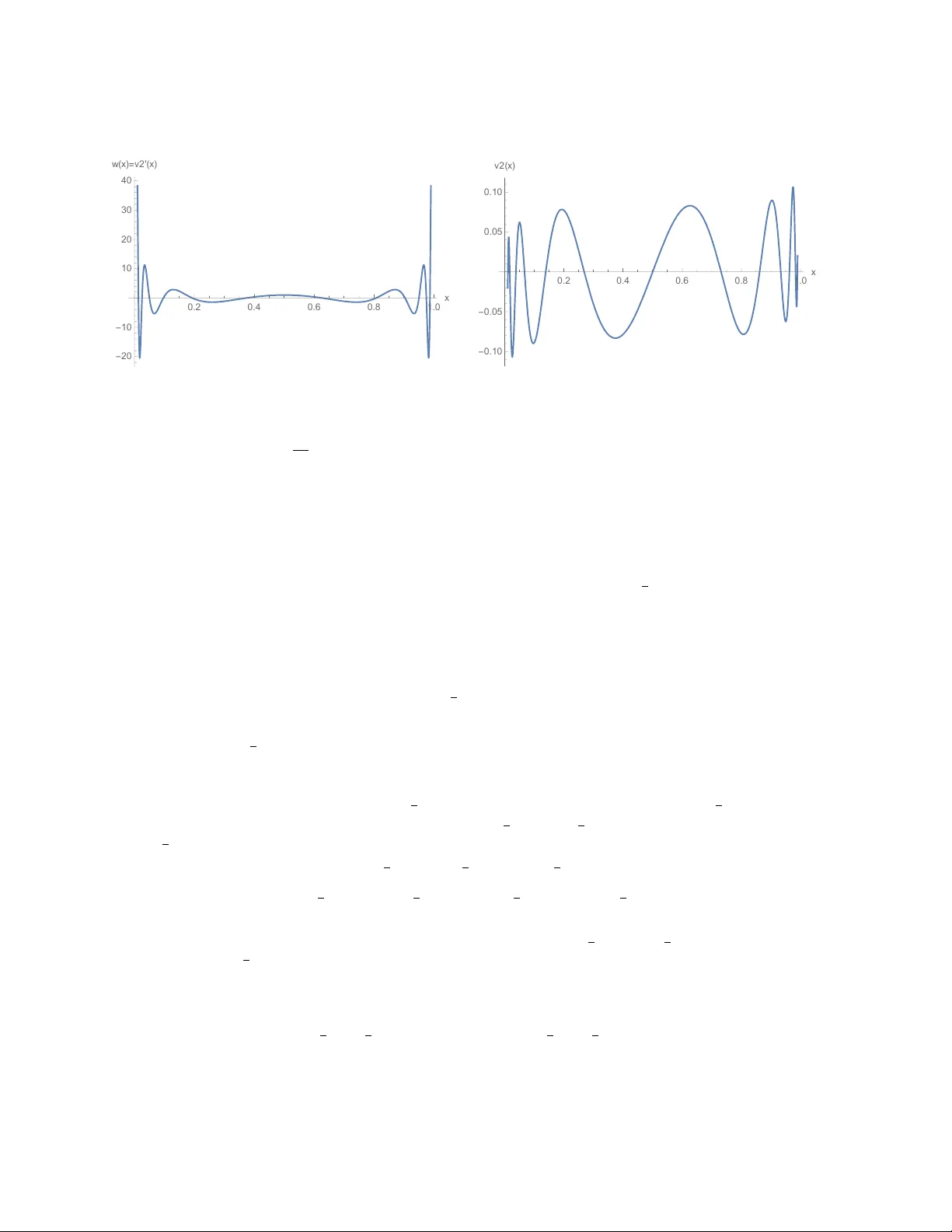
In v erse Sp ectral Analysis of Singular Radial AKNS Op erators Damien Gobin, Benoît Gréb ert, Bernard Helffer and F rançois Nicoleau Abstract W e study an in verse spectral problem for singular AKNS op erators based on sp ectral data asso- ciated with tw o distinct v alues of the effective angular momentum parameter κ . Our main fo cus is the lo cal in v erse problem near the zero p otential. F or the pairs ( κ 1 , κ 2 ) = (0 , 1) , (1 , 2) and (0 , 3) , w e establish local uniqueness. F or (0 , 2) , we prov e that the F réchet differential of the sp ectral map at the origin is injective, while the question whether its range is closed remains open. 1 In tro duction In verse sp ectral theory for one-dimensional singular differen tial operators arises naturally in the analysis of radially symmetric quan tum systems. The classical example is the radial Schrödinger op erator, obtained from the three-dimensional Schrödinger equation after separation of v ariables in spherical c oordinates. F or a real-v alued square-integrable p oten tial q ∈ L 2 (0 , 1) , the radial equation tak es the form H ℓ ( q ) u := − d 2 u dx 2 + ℓ ( ℓ + 1) x 2 u + q ( x ) u = λu , x ∈ (0 , 1) , ℓ ∈ N . (1.1) The regularit y condition is u ( x ) = O ( x ℓ +1 ) as x → 0 , together with the Dirichlet boundary condition u (1) = 0 . F or each angular momentum ℓ , this defines a self-adjoint op erator on L 2 (0 , 1) with discrete, simple, real sp ectrum. The inv erse sp ectral problem consists in determining the p otential q ( x ) from its spectral data. A classi- cal result due to Pösc hel–T rub o witz [28], Carlson [11], Guillot–Ralston [16] and Zhornitsk ay a–Sero v [38] asserts that the Diric hlet spectrum together with suitable norming constants forms a real-analytic co or- dinate system on L 2 (0 , 1) for each fixed ℓ . Recen tly , in the context of radial Schrödinger operators with distinct angular momen ta, w e pro ved in [14] that the p otential is uniquely determined b y the Dirichlet sp ectra corresp onding to infinitely man y v alues of ℓ satisfying a Mün tz-type condition, and that in a neigh b orho od of the zero p oten tial, kno wing tw o spectra (for the pairs ( ℓ 1 , ℓ 2 ) = (0 , 1) , (1 , 2) or (0 , 3) ) already implies uniqueness. These results rely on the explicit structure of the eigenfunctions in terms of Bessel functions, sp ecifically of the form u ℓ,n ( x ) = c ℓ,n x 1 / 2 J ν ( j ν,n x ) , ν = ℓ + 1 2 , (1.2) together with delicate completeness prop erties of the squared eigenfunctions , following earlier works of Rundell and Sacks [29]. The aim of the presen t work is to inv estigate the analog of this sp ectral problem for singular radial AKNS op erators. The mathematical mo del considered here arises from certain ph ysical mo dels, whose deriv ation is briefly outlined in the app endix. After separation of v ariables, one is led to a family of singular radial AKNS op erators parameterized by what we call an effe ctive angular momentum p ar ameter κ ∈ Z . W e 1 emphasize that the parameter κ do es not, in general, corresp ond to a genuine angular momentum, in con trast with the Schrödinger case. In the 3D Dirac framework, − κ arises as an eigen v alue of the spin– orbit op erator K , whereas in the 2D mo del it can b e in terpreted as an effectiv e angular momentum (see (7.97) in [36] and App endix A of the present pap er). The asso ciated singular AKNS op erator is H κ ( V ) Z = H κ ( p, q ) Z =  0 − 1 1 0  Z ′ +   0 − κ x − κ x 0   Z + V ( x ) Z , Z = ( Z 1 , Z 2 ) T . (1.3) Here the p oten tial matrix V is given by V ( x ) =  − q ( x ) p ( x ) p ( x ) q ( x )  , p, q ∈ L 2 R (0 , 1) . (1.4) W e imp ose the follo wing b oundary conditions. Let ( θ 1 , θ 2 ) ∈ R 2 . • When κ = 0 , Z (0) · u θ 1 = 0 , Z (1) · u θ 2 = 0 , u θ j =  sin θ j cos θ j  . (1.5) • When κ  = 0 , Z (1) · u θ 2 = 0 . (1.6) The AKNS system enjo ys symmetries associated with the Pauli matrices σ 1 =  0 1 1 0  , σ 2 =  0 − i i 0  , σ 3 =  1 0 0 − 1  . (1.7) A direct computation sho ws that σ 1 H κ ( p, q ) σ 1 = − H − κ ( − p, q ) , (1.8) σ 2 H κ ( p, q ) σ 2 = H − κ ( − p, − q ) , (1.9) σ 3 H κ ( p, q ) σ 3 = − H κ ( p, − q ) . (1.10) In particular, if Z solv es H κ ( p, q ) Z = λZ , then σ 1 Z , σ 2 Z and σ 3 Z solv e the corresp onding transformed systems with the same or opp osite sp ectral parameter according to (1.8)–(1.10). In the case p = 0 , the σ 1 -symmetry sho ws that the kno wledge of the spectra corresp onding to κ and − κ (with the same b oundary condition θ 2 = 0 ) is equiv alent, up to a reindexation, to the knowledge of the tw o sp ectra asso ciated with θ 2 = 0 and θ 2 = π / 2 for H κ . Therefore, pro vided that the resulting sequences satisfy the technical interlacing property required in Theorem 1.1 of [3], the p oten tial q is uniquely determined. F or these reasons, and other tec hnical difficulties 1 , we restrict ourselv es, in the present pap er, to the case κ ≥ 0 and θ 2 = 0 . 1 It would actually be in teresting to treat the general case, but, except for the case θ 2 = π 2 , this would indeed be technically more in volv ed. 2 In the case κ = 0 , we also set θ 1 = 0 . As explained in the appendix, θ 2 = 0 corresponds in the motiv ating Dirac radial mo del to the so-called Zig–Zag condition, while the MIT bag condition corresponds to θ 2 = ± π 4 . The domain of the op erator is then defined as follows: D ( H 0 ) = n Z = ( Z 1 , Z 2 ) ∈ L 2 (0 , 1) 2 : H 0 Z ∈ L 2 (0 , 1) 2 , Z 2 (0) = 0 , Z 2 (1) = 0 o . (1.11) F or κ > 0 , we set D ( H κ ) = n Z = ( Z 1 , Z 2 ) ∈ L 2 (0 , 1) 2 : H κ Z ∈ L 2 (0 , 1) 2 , Z 2 (1) = 0 o . (1.12) As sho wn in [32], this realizes a self-adjoin t op erator with purely discrete and simple sp ectrum whic h can b e written as a doubly infinite sequence { λ κ,n ( p, q ) } n ∈ Z , (1.13) ordered as · · · < λ κ, − 2 ( p, q ) < λ κ, − 1 ( p, q ) < λ κ, 0 ( p, q ) < λ κ, 1 ( p, q ) < λ κ, 2 ( p, q ) < · · · . (1.14) The lab elling is uniquely determined by the asymptotic b ehavior (see [32], Theorem 3.1): λ κ,n ( p, q ) =  n + sgn( n ) κ 2  π + ℓ 2 ( n ) , as | n | → ∞ , (1.15) whic h gov erns b oth ends of the sequence. Here the notation α n = β n + ℓ 2 ( n ) , n ∈ Z , means that the sequence ( α n − β n ) n ∈ Z b elongs to ℓ 2 ( Z ) . In addition to the eigenv alues, Serier introduced suitable norming constants whic h, together with the sp ectrum, form a complete system of sp ectral coordinates. More precisely , the combined data (eigenv alues and norming constan ts) pro vide a lo cally stable parameterization of the p otential and yield a Borg– Levinson type uniqueness result (see [32]). Ho wev er, these classical results rely crucially on the av ailability of norming constants. F rom the physical and inv erse point of view, suc h quan tities are in general not observable . This naturally leads to a differen t and more c hallenging question: can one determine the potential uniquely from sp ectral data alone, without an y norming constan ts? As in the corresponding inv erse problem for the radial Sc hrö dinger operator, the spectral data asso ciated with a single effectiv e angular momentum are not sufficien t to ensure uniqueness. This naturally leads to com bining information from at le ast two distinct effe ctive angular momenta κ . More precisely , w e consider the sp ectra corresponding to tw o distinct effective angular momenta κ 1  = κ 2 and study whether this purely sp ectral information, without any norming constants, determines the p oten tial. W e now state our first main result, which gives several cases where tw o spectra are sufficient to reco ver the p oten tial lo cally near the trivial configuration. Theorem 1.1 (Lo cal uniqueness for the pairs (0 , 1) , (1 , 2) and (0 , 3) ) . L et ( κ 1 , κ 2 ) = (0 , 1) , (1 , 2) or (0 , 3) . Then the know le dge of the sp e ctr a asso ciate d with the effe ctive angular momenta κ 1 and κ 2 uniquely determines the p otential V = ( p, q ) ∈ L 2 (0 , 1) × L 2 (0 , 1) in a neighb orho o d of the zer o p otential V 0 = 0 . 3 The pro of of Theorem 1.1 relies on the analysis of the F réchet differential of the asso ciated sp ectral map at the zero p oten tial. W e show that this differen tial is injectiv e with closed range, which yields the desired lo cal uniqueness result. W e no w briefly in tro duce this spectral map. Let e λ κ,n ( p, q ) denote the renormalized eigenv alues, implicitly defined by the asymptotic form ula (1.15) and explicitly given b y e λ κ,n ( p, q ) = λ κ,n ( p, q ) −  n + sgn( n ) κ 2  π . W e choose tw o distinct effective angular momenta κ 1  = κ 2 , whic h are fixed integers and we consider the asso ciated sp ectral map S κ 1 ,κ 2 : L 2 (0 , 1) × L 2 (0 , 1) − → ℓ 2 R ( Z ) × ℓ 2 R ( Z ) , defined by S κ 1 ,κ 2 ( p, q ) =   e λ κ 1 ,n ( p, q )  n ∈ Z ,  e λ κ 2 ,n ( p, q )  n ∈ Z  . (1.16) W e no w state the second main result of this pap er, which discusses the injectivit y of the F réchet differen tial of the sp ectral map at the zero p oten tial for three pairs of effective angular momenta. Theorem 1.2 (Behavior of the differential of the sp ectral map) . L et κ 1  = κ 2 b e two distinct inte gers and c onsider the sp e ctr al map S κ 1 ,κ 2 : L 2 (0 , 1) × L 2 (0 , 1) − → ℓ 2 R ( Z ) × ℓ 2 R ( Z ) . Then, at the zer o p otential V = 0 , the F r é chet differ ential of S κ 1 ,κ 2 satisfies: • F or ( κ 1 , κ 2 ) = (0 , 1) , (1 , 2) or (0 , 3) , the differ ential is inje ctive and has close d r ange. • F or ( κ 1 , κ 2 ) = (0 , 2) , the differ ential is inje ctive. The pro of of Theorem 1.2 is given in Sections 6–7. The case (0 , 2) remains op en, as we hav e not b een able to prov e that the differential has closed range. Theorem 1.1 then follows from the local injectivit y result stated in Proposition 7.2. In the app endix, we will describ e ho w these questions arise in the analysis of inv erse sp ectral problems for the radial Dirac op erator (with p ossible addition of an Aharonov–Bohm p oten tial) in dimension tw o and three and presen t some remaining op en questions. 2 Eigen v alue analysis in the unp erturb ed case V = 0 In this section we analyze the sp ectral problem in the unp erturbed case V = 0 , whic h serves as the reference configuration for the p erturbativ e and inv erse analysis developed later. When V = 0 , the AKNS op erator reduces to the first-order matrix equation 0 − 1 1 0 ! Z ′ ( x ) +   0 − κ x − κ x 0   Z ( x ) = λZ ( x ) , x ∈ (0 , 1) , (2.1) with the b oundary condition Z 2 (0) = 0 , Z 2 (1) = 0 for κ = 0 , Z 2 (1) = 0 , for κ  = 0 . (2.2) 4 2.1 The case λ = 0 The case λ = 0 requires a sp ecific discussion. Setting λ = 0 in the unp erturbed Dirac equation yields Z ′ 1 = κ x Z 1 , Z ′ 2 = − κ x Z 2 . Hence the general solutions are Z 1 ( x ) = C 1 x κ , Z 2 ( x ) = C 2 x − κ . F or κ = 0 , the b oundary condition Z 2 (0) = 0 forces C 2 = 0 . F or κ ≥ 1 , the condition Z 2 ∈ L 2 (0 , 1) near x = 0 again forces C 2 = 0 . so that Z ( x ) =  C 1 x κ 0  . The b oundary condition at x = 1 is satisfied, and therefore 0 is an eigen v alue of H κ (0) . The associated eigenfunction is thus giv en by Z (0) κ, 0 ( x ) = c κ, 0  x κ 0  , c κ, 0 > 0 , and the normalization condition ∥ Z (0) κ, 0 ∥ L 2 (0 , 1) 2 = 1 , yields c κ, 0 = √ 2 κ + 1 , so that Z (0) κ, 0 ( x ) = √ 2 κ + 1  x κ 0  . 2.2 The case λ  = 0 W e no w consider the case λ  = 0 , for which the system (2.1) decouples into t wo scalar equations for Z 1 and Z 2 :          Z ′′ 1 ( x ) +  λ 2 − κ ( κ − 1) x 2  Z 1 ( x ) = 0 , Z ′′ 2 ( x ) +  λ 2 − κ ( κ + 1) x 2  Z 2 ( x ) = 0 . (2.3) W e set ν = κ + 1 2 . After the standard substitution Z j ( x ) = √ x u j ( λx ) , the system reduces to Bessel equations of orders ν − 1 and ν . A ccordingly , a fundamental system of solutions is giv en by Z (0) ( x, λ ) = r π λx 2 J ν − 1 ( λx ) − J ν ( λx ) ! , W (0) ( x, λ ) = r π λx 2 − Y ν − 1 ( λx ) Y ν ( λx ) ! . (2.4) where J ν and Y ν denote the Bessel functions of the first and second kinds (see [21]). W e recall that for z ∈ C \ ( −∞ , 0] and any real or complex parameter ν , one has J ν ( z ) =  z 2  ν ∞ X k =0 ( − 1) k  z 2 4  k k ! Γ( ν + k + 1) . (2.5) F or ν / ∈ Z , the function Y ν is given by 2 2 F or an integer n , the function Y n ( z ) is defined b y the limit Y n ( z ) = lim ν → n Y ν ( z ) . 5 Y ν ( z ) = J ν ( z ) cos( ν π ) − J − ν ( z ) sin( ν π ) . (2.6) W e emphasize that for half-in teger orders ν ∈ 1 2 + N , the function √ z J ν ( z ) is entire, whereas √ z Y ν ( z ) is generally meromorphic because of its singularity at z = 0 . As x → 0 , these functions satisfy the classical asymptotics : J ν ( x ) ∼ 1 Γ( ν + 1)  x 2  ν , Y ν ( x ) ∼ − Γ( ν ) π  2 x  ν , ν > 0 . (2.7) Hence J ν is regular at the origin, whereas Y ν is singular. In particular, among the tw o fundamen tal solutions in (2.4), only Z (0) ( x, λ ) is square–in tegrable near x = 0 and satisfies the regularity condition. F or each eigenv alue λ = λ κ,n (0 , 0) of the unp erturbed op erator, we define the associated eigenfunction b y Z (0) κ,n ( x ) = c κ,n Z (0) 1 ,κ,n ( x ) Z (0) 2 ,κ,n ( x ) ! = c κ,n q λ κ,n (0 , 0) x J ν − 1  λ κ,n (0 , 0) x  − J ν  λ κ,n (0 , 0) x  ! , (2.8) where c κ,n > 0 is a normalization constant to be sp ecified later. Using the b oundary condition at x = 1 , w e obtain that the eigen v alues of H κ (0) are the simple zeros of J ν , as will be detailed in the paragraph b elo w. 2.3 Symmetries In this paragraph w e recall the symmetry prop erties of the unp erturb ed sp ectrum for V = 0 . F or half–integer orders ν = κ + 1 2 , the en tire function z 7→ √ z J ν ( z ) is an even function when κ is odd, and an o dd function when κ is even. This parity prop ert y immediately yields the following symmetry for the nonzero eigenv alues: λ κ, − n (0 , 0) = − λ κ,n (0 , 0) , for n ≥ 1 . (2.9) W e recall that the b oundary condition leads to the characteristic equation J ν ( λ ) = 0 . If { j ν,n } n ≥ 1 denotes the sequence of p ositiv e zeros of J ν , then the nonzero eigen v alues of H κ (0) are λ κ, ± n (0 , 0) = ± j ν,n , n ≥ 1 . (2.10) Moreo ver, we hav e seen that λ = 0 is an eigen v alue. Thus the full sp ectrum is symmetric and ordered as · · · < − j ν, 2 < − j ν, 1 < 0 < j ν, 1 < j ν, 2 < · · · , (2.11) and we assign λ = 0 to the index n = 0 in the bi-infinite en umeration { λ κ,n (0) } n ∈ Z . 2.4 Summary and notation The sp ectrum of the unp erturbed op erator H κ (0) consists of the simple eigen v alue λ κ, 0 (0) = 0 and of the nonzero eigenv alues λ κ, ± n (0) = ± j ν,n for n ≥ 1 , forming a symmetric bi-infinite sequence indexed b y n ∈ Z (see (2.11)). This enumeration is consisten t with the asymptotic formula (1.15) (see [26], 10.21 (vi)). 6 The asso ciated eigenfunctions are given b y the regular solutions Z (0) κ,n . F or the zero eigen v alue, one has Z (0) κ, 0 ( x ) = √ 2 κ + 1  x κ 0  , while for n  = 0 they are expressed in terms of Bessel functions. By symmetry , the eigenfunctions corresponding to λ κ,n (0) and λ κ, − n (0) differ only by a sign in their oscillatory comp onen ts. In particular, the normalization constants dep end only on | n | , and c κ, − n = c κ,n , for n ≥ 1 . A ccordingly , we index the sp ectrum by n ∈ Z , with n = 0 correspondin g to the zero eigenv alue. Remark 2.1 (Normalization constan ts) . W e wil l ne e d the asymptotic b ehavior of these normalization c onstants as n → ∞ (se e Se ction 3.3). In fact, the c onstants c κ,n c an b e c ompute d explicitly using the fol lowing standar d finite-interval identity (often r eferr e d to as a Lommel-type formula, se e ([26], 10.22.5)): for any α , µ ∈ R + , Z 1 0 x J µ ( αx ) 2 dx = 1 2  J µ ( α ) 2 − J µ − 1 ( α ) J µ +1 ( α )  . (2.12) Applying (2.12) with α = j ν, | n | and µ = ν , and using J ν ( j ν, | n | ) = 0 to gether with the r e curr enc e J ν − 1 ( α ) + J ν +1 ( α ) = 2 ν α J ν ( α ) , we obtain J ν − 1 ( j ν, | n | ) = − J ν +1 ( j ν, | n | ) and henc e Z 1 0 x J ν  j ν, | n | x  2 dx = 1 2 J ν +1  j ν, | n |  2 . Similarly, applying (2.12) with µ = ν − 1 yields Z 1 0 x J ν − 1  j ν, | n | x  2 dx = 1 2 J ν − 1  j ν, | n |  2 = 1 2 J ν +1  j ν, | n |  2 . Substituting these identities into the normalization c ondition ∥ Z (0) κ,n ∥ L 2 (0 , 1) 2 = 1 (se e (2.8) ) gives c κ,n = 1 p j ν, | n |   J ν +1 ( j ν, | n | )   , as n  = 0 . (2.13) The classic al asymptotic exp ansions for Bessel functions and for their p ositive zer os j ν,n (se e, e.g., W at- son [37]) yield c 2 κ,n = π 2 + 4 ν 2 − 1 16 π  n + ν / 2 − 1 / 4  2 + O  n − 4  , n → ∞ . (2.14) Final ly, in the zer o-eigenvalue c ase, we r e c al l that the normalization c ondition yields c κ, 0 = √ 2 κ + 1 . W e conclude this section with the explicit analysis of the sp ecial case κ = 0 . In this case, the computations are particularly simple and allo w us to illustrate the preceding constructions in a fully explicit manner. 7 2.5 The case κ = 0 W e now consider the case κ = 0 , for whic h ν = 1 2 and the singular term κ/x disapp ears from the system. The analysis of this particular case is especially interesting (s ee Section 3.4). In this setting, the Dirac system (2.1) reduces to Z ′ 1 = λ Z 2 , Z ′ 2 = − λ Z 1 , and the regular solution, c haracterized b y the condition Y 2 (0) = 0 , is given b y Z (0) ( x, λ ) =  cos( λx ) − sin( λx )  . Imp osing the b oundary condition at x = 1 yields the characteristic equation sin( λ ) = 0 , so that the nonzero eigenv alues are explicitly giv en by λ 0 ,n (0 , 0) = nπ , n ∈ Z \ { 0 } . (2.15) F or eac h n ∈ Z , the asso ciated eigenfunction is Z (0) 0 ,n ( x ) =  cos( nπ x ) − sin( nπ x )  , (2.16) since the L 2 (0 , 1) 2 -norm of this v ector-v alued function equals 1 . Remark 2.2. R e c al l that the Bessel functions of or der 1 2 admit the elementary r epr esentations J 1 / 2 ( z ) = r 2 π z sin z , J − 1 / 2 ( z ) = r 2 π z cos z . (2.17) 3 Sp ectral map and the linearized problem at V = 0 . In this section we in tro duce the sp ectral map and analyze its linearization at the unp erturbed config- uration V = 0 . This linearized analysis provides the key to ol for the local inv erse results established later. 3.1 Differen tial of λ κ,n ( p, q ) and the sp ectral map In this subsection w e recall the analytic dep endence of the eigenv alues on the AKNS p oten tial V = ( p, q ) and describ e their F réc het differen tial. F ollowing Serier [32, Prop. 3.1], for each fixed pair ( κ, n ) ∈ N × Z the map ( p, q ) ∈ L 2 (0 , 1) × L 2 (0 , 1) 7− → λ κ,n ( p, q ) is real-analytic. Moreov er, if λ κ,n ( p, q ) is a simple eigen v alue of H κ ( V ) with normalized eigenfunction Z κ,n ( x ; p, q ) =  Z 1 ,κ,n ( x ; p, q ) Z 2 ,κ,n ( x ; p, q )  , ∥ Z κ,n ( · ; p, q ) ∥ L 2 (0 , 1) 2 = 1 , 8 then the F réchet differential at ( p, q ) in the direction ( v 1 , v 2 ) ∈ L 2 (0 , 1) × L 2 (0 , 1) is given b y D ( p,q ) λ κ,n ( p, q ) · ( v 1 , v 2 ) = Z 1 0  2 Z 1 ,κ,n ( x ; p, q ) Z 2 ,κ,n ( x ; p, q ) v 1 ( x ) +  Z 2 ,κ,n ( x ; p, q ) 2 − Z 1 ,κ,n ( x ; p, q ) 2  v 2 ( x )  dx . (3.1) The relation (3.1) therefore allows us to compute the differential of the sp ectral map in tro duced in (1.16). 3.2 The linearized problem at V = 0 W e now inv estigate the F réchet deriv ative of the sp ectral map at the unperturb ed potential V = 0 , which leads to the formulation of the linearized inv erse problem. Our ob jective is to determine whether, for tw o distinct effective angular momen ta κ 1  = κ 2 , the asso ciated map V = ( p, q ) 7− →  λ κ 1 ,n ( p, q ) , λ κ 2 ,n ( p, q )  n ∈ Z is lo cally injective at V = 0 . Equiv alently , the same question can b e form ulated in terms of the renor- malized eigen v alues e λ κ,n , since the renormalization consists in subtracting an explicit function of n which is indep enden t of ( p, q ) and therefore do es not affect the F réchet differential at V = 0 . F rom the general v ariation formula (3.1), one obtains D ( p,q ) λ κ,n (0 , 0) · ( v 1 , v 2 ) = Z 1 0  2 Z (0) 1 ,κ,n ( x ) Z (0) 2 ,κ,n ( x ) v 1 ( x ) +  Z (0) 2 ,κ,n ( x )  2 −  Z (0) 1 ,κ,n ( x )  2  v 2 ( x )  dx , (3.2) where Z (0) κ,n ( x ) = Z (0) 1 ,κ,n ( x ) Z (0) 2 ,κ,n ( x ) ! , is the normalized eigenfunction of H κ (0) asso ciated with the eigenv alue λ κ,n (0 , 0) . W e begin with the case of nonzero eigen v alues. Using the results of the previous sections and the symmetry prop erties of the unp erturbed sp ectrum, we obtain for every n ∈ Z ± D ( p,q ) λ κ,n (0 , 0) · ( v 1 , v 2 ) = c 2 κ, | n | Z 1 0 j ν, | n | x  ∓ 2 J ν − 1  j ν, | n | x  J ν  j ν, | n | x  v 1 ( x ) +  J ν  j ν, | n | x  2 − J ν − 1  j ν, | n | x  2  v 2 ( x )  dx . (3.3) W e next consider the zero eigen v alue. Recalling that Z (0) κ, 0 ( x ) = c κ, 0  x κ 0  , c κ, 0 = √ 2 κ + 1 , substituting this expression in to (3.1) yields D ( p,q ) λ κ, 0 (0 , 0) · ( v 1 , v 2 ) = − (2 κ + 1) Z 1 0 x 2 κ v 2 ( x ) dx . (3.4) The structure of system (3.3) suggests that the con tributions of v 1 and v 2 can b e separated. W e no w formalize this observ ation by introducing a b ounded isomorphism on the target space whic h exactly decouples the differential of the sp ectral map. 9 3.3 Decoupling of the differential via a contin uous isomorphism W e sho w that, up to a b ounded isomorphism on the target space, the differential of the sp ectral map can b e reduced to a fully decoupled system. This allows us to study indep endently the contributions of v 1 and v 2 . W e denote this differen tial by S := D ( p,q ) S κ 1 ,κ 2 (0 , 0) . Notation. F or each κ ∈ { κ 1 , κ 2 } and eac h n ≥ 1 (with ν = κ + 1 2 ), w e in tro duce the b ounded linear functionals on L 2 (0 , 1) A κ,n ( v 1 ) := Z 1 0 2 j ν,n x J ν − 1  j ν,n x  J ν  j ν,n x  v 1 ( x ) dx , B κ,n ( v 2 ) := Z 1 0 j ν,n x  J ν  j ν,n x  2 − J ν − 1  j ν,n x  2  v 2 ( x ) dx . In this notation, for n ≥ 1 , D ( p,q ) λ κ, ± n (0 , 0) · ( v 1 , v 2 ) = c 2 κ,n  ∓ A κ,n ( v 1 ) + B κ,n ( v 2 )  , while for the zero mo de one has D ( p,q ) λ κ, 0 (0 , 0) · ( v 1 , v 2 ) = − c 2 κ, 0 Z 1 0 x 2 κ v 2 ( x ) dx , c κ, 0 = √ 2 κ + 1 . (3.5) F or κ ∈ { κ 1 , κ 2 } , define d κ ( v ) :=  d κ,n ( v )  n ∈ Z :=  D ( p,q ) λ κ,n (0 , 0) · v  n ∈ Z ∈ ℓ 2 ( Z ) , v = ( v 1 , v 2 ) , so that S ( v ) = ( d κ 1 ( v ) , d κ 2 ( v )) ∈ ℓ 2 ( Z ) × ℓ 2 ( Z ) . No w, for fixed κ , define the linear map U κ : ℓ 2 ( Z ) − → R × ℓ 2 ( N ∗ ) × ℓ 2 ( N ∗ ) b y U κ ( a ) = a 0 c 2 κ, 0 ,  a − n − a n 2 c 2 κ,n  n ≥ 1 ,  a − n + a n 2 c 2 κ,n  n ≥ 1 ! , (3.6) where N ∗ := { 1 , 2 , 3 , . . . } denotes the set of p ositive in tegers. Using (2.14), w e see that ( c κ,n ) n ∈ Z is uniformly b ounded ab ov e and b elo w, so U κ is a b ounded isomorphism. Applying U κ to d κ ( v ) and using the formulas ab o ve yields the exact decoupling U κ  d κ ( v )  =  − Z 1 0 x 2 κ v 2 ,  A κ,n ( v 1 )  n ≥ 1 ,  B κ,n ( v 2 )  n ≥ 1  . (3.7) 10 Finally , set U := U κ 1 × U κ 2 , which is a b ounded isomorphism on ℓ 2 ( Z ) × ℓ 2 ( Z ) . Then ( U ◦ S )( v 1 , v 2 ) =  M ( v 2 ) , A κ 1 ,κ 2 ( v 1 ) , B κ 1 ,κ 2 ( v 2 )  , (3.8) where M ( v 2 ) =  − Z 1 0 x 2 κ 1 v 2 , − Z 1 0 x 2 κ 2 v 2  ∈ R 2 , and A κ 1 ,κ 2 ( v 1 ) =  ( A κ 1 ,n ( v 1 )) n ≥ 1 , ( A κ 2 ,n ( v 1 )) n ≥ 1  , B κ 1 ,κ 2 ( v 2 ) =  ( B κ 1 ,n ( v 2 )) n ≥ 1 , ( B κ 2 ,n ( v 2 )) n ≥ 1  . In particular, U ◦ S is block diagonal: v 1 only enters A κ 1 ,κ 2 , whereas v 2 only enters ( M , B κ 1 ,κ 2 ) . 3.4 Reform ulation of the injectivity problem W e now reformulate the injectivity of the F réc het differential of the spectral map S κ 1 ,κ 2 at ( p, q ) = (0 , 0) . By definition, injectivity amoun ts to c haracterizing all p erturbations ( v 1 , v 2 ) such that S ( v 1 , v 2 ) = 0 , S = D ( p,q ) S κ 1 ,κ 2 (0 , 0) . Since U is a b ounded isomorphism on the target space, this condition is equiv alent to ( U ◦ S )( v 1 , v 2 ) = 0 . Using the blo c k diagonal structure (3.8), the k ernel condition reduces to the decoupled system A κ 1 ,κ 2 ( v 1 ) = 0 , M ( v 2 ) = 0 , B κ 1 ,κ 2 ( v 2 ) = 0 . (3.9) This decoupling also reflects the choice of b oundary conditions, which is encoded in the structure of the eigenfunctions. Th us, the study of the kernel separates in to tw o indep enden t problems: one inv olving only the comp onen t v 1 , go verned by A κ 1 ,κ 2 , and one inv olving only the comp onen t v 2 , go verned by ( M , B κ 1 ,κ 2 ) . F or a fixed effective angular momentum κ , the ab o v e conditions reduce to A κ,n ( v 1 ) = 0 , n ≥ 1 , B κ,n ( v 2 ) = 0 , n ≥ 1 , Z 1 0 x 2 κ v 2 ( x ) dx = 0 . (3.10) As an illustration, consider the simple case κ = 0 . Using the explicit expressions of the Bessel functions of order ± 1 2 , one obtains x J − 1 / 2 ( nπ x ) J 1 / 2 ( nπ x ) = 1 2 sin(2 nπ x ) , x  J 1 / 2 ( nπ x ) 2 − J − 1 / 2 ( nπ x ) 2  = − cos(2 nπ x ) . Hence (3.10) b ecomes Z 1 0 sin(2 nπ x ) v 1 ( x ) dx = 0 , n ≥ 1 , and Z 1 0 cos(2 nπ x ) v 2 ( x ) dx = 0 , n ≥ 1 , Z 1 0 v 2 ( x ) dx = 0 . These relations show that v 1 is ev en and v 2 is odd with resp ect to x = 1 2 . Conv ersely , if v 1 is ev en and v 2 is o dd with resp ect to x = 1 2 , then all the ab o v e integrals v anish. Hence these parity conditions are necessary and sufficient for S ( v 1 , v 2 ) = 0 in the case κ = 0 . 11 4 Kneser–Sommerfeld–T yp e Expansions The classical Kneser–Sommerfeld iden tity provides a series expansion ov er the zeros j ν,n of J ν . Its correct form, first given by Buc hholz [9] and later clarified b y Ha yashi [17] and Martin [23], differs from the formula stated b y W atson, which omits an essen tial in tegral term. The v alid expansion (4.1) pla yed a central role in our previous analysis of the radial Schrödinger operator: X n ≥ 1 J ν ( j ν,n x ) J ν ( j ν,n X ) ( z 2 − j 2 ν,n ) [ J ′ ν ( j ν,n )] 2 = π 4 J ν ( z ) J ν ( xz )  J ν ( z ) Y ν ( X z ) − Y ν ( z ) J ν ( X z )  , (4.1) for 0 < x ≤ X ≤ 1 . In the presen t AKNS setting, the linearized system (3.3) inv olves b oth squared and mixed Bessel pro ducts. The relev an t combinations are, with ν = κ + 1 2 , J ν ( j ν,n x ) 2 , J ν − 1 ( j ν,n x ) 2 and J ν − 1 ( j ν,n x ) J ν ( j ν,n x ) . Ho wev er, the last t wo expressions fall outside the framew ork of the classical Kneser–Sommerfeld expan- sion, which treats only diagonal pro ducts of the form J ν ( xj ν,n ) J ν ( X j ν,n ) . T o handle the AKNS structure, we therefore require mo difie d Kneser–Sommerfeld–t yp e iden tities. In what follows, we no w state three additional identities of the same t yp e. F or simplicit y , we assume that ν ∈ R + \ N , although the form ulas extend to arbitrary complex v alues of ν . 3 Prop osition 4.1. L et ν ∈ R + \ N , z  = 0 , z  = j ν,n and 0 < x ≤ X ≤ 1 . The fol lowing Kneser– Sommerfeld–typ e identities hold: X n ≥ 1 J ν − 1 ( j ν,n x ) J ν − 1 ( j ν,n X ) ( z 2 − j 2 ν,n )  J ′ ν ( j ν,n )  2 = − ν z 2 ( xX ) ν − 1 + π 4 J ν ( z ) J ν − 1 ( xz )  J ν ( z ) Y ν − 1 ( X z ) − Y ν ( z ) J ν − 1 ( X z )  , (4.2) X n ≥ 1 J ν − 1 ( j ν,n x ) J ν ( j ν,n X ) ( z 2 − j 2 ν,n ) j ν,n  J ′ ν ( j ν,n )  2 = 1 2 z 2 x ν − 1 ( X − ν − X ν ) + π 4 z J ν ( z ) J ν − 1 ( xz )  J ν ( z ) Y ν ( X z ) − Y ν ( z ) J ν ( X z )  , (4.3) X n ≥ 1 J ν − 1 ( j ν,n X ) J ν ( j ν,n x ) ( z 2 − j 2 ν,n ) j ν,n  J ′ ν ( j ν,n )  2 = − 1 2 z 2 x ν X ν − 1 + π 4 z J ν ( z ) J ν ( xz )  J ν ( z ) Y ν − 1 ( X z ) − Y ν ( z ) J ν − 1 ( X z )  . (4.4) Pr o of. W e follow, step b y step, the con tour-in tegral argumen t of W atson for the Kneser-Sommerfeld form ula (see [37]), in the corrected form later clarified by Buchholz, Hay ashi and Martin. W e first giv e the pro of of (4.2). 3 Here w e use the definition of Y n ( z ) recalled ab o ve. 12 Let z ∈ C with, for instance, ℜ z > 0 and z  = j ν,n for all n ≥ 1 . F ollowing W atson’s approac h, w e in tro duce, for w ∈ C and fixed 0 < X ≤ 1 , the auxiliary function W ν ( w , X ) := J ν ( w ) Y ν − 1 ( X w ) − Y ν ( w ) J ν − 1 ( X w ) . (4.5) Using the small- w asymptotics of J ν and Y ν (see (2.7)), one readily obtains W ν ( w , X ) = 2 X ν − 1 π w + O (1) , w → 0 . (4.6) Recall the Hankel functions H (1) ν ( w ) = J ν ( w ) + i Y ν ( w ) , H (2) ν ( w ) = J ν ( w ) − i Y ν ( w ) . (4.7) A short computation giv es the equiv alent represen tation W ν ( w , X ) = − 1 2 i h H (1) ν ( w ) H (2) ν − 1 ( X w ) − H (2) ν ( w ) H (1) ν − 1 ( X w ) i . (4.8) Finally , from the large- w asymptotics ([21], (5.11.4)-(5.11.5)), v alid for | arg w | ≤ π − δ , δ ∈ (0 , π ) , H (1) ν ( w ) ∼ r 2 π w e i ( w − ν π 2 − π 4 ) , H (2) ν ( w ) ∼ r 2 π w e − i ( w − ν π 2 − π 4 ) , (4.9) w e obtain, for | w | large with ℜ w > 0 , | W ν ( w , X ) | ≲ e (1 − X ) |ℑ w | | w | , 0 < X ≤ 1 . (4.10) W e consider the contour in tegral I B ,M,ϵ = I C B,M ,ϵ W ν ( w , X ) w 2 − z 2 w J ν − 1 ( xw ) J ν ( w ) dw , (4.11) where C B ,M,ϵ is the rectangle in the half-plane ℜ w ≥ 0 , with v ertices ± iB , ± iB + M π + (2 ν + 1) π 4 , for B > 0 and M ∈ N large enough, indented at the origin with a half-circle of radius ϵ > 0 in the half-plane ℜ w > 0 : 13 ℜ w ℑ w iB − iB iB + M π + (2 ν +1) π 4 − iB + M π + (2 ν +1) π 4 iϵ − iϵ ϵ 0 z C B ,M,ϵ Using again the small- w asymptotics of J ν and Y ν (see (2.7)), one readily obtains W ν ( w , X ) w 2 − z 2 w J ν − 1 ( xw ) J ν ( w ) = − 4 ν π z 2 w ( xX ) ν − 1 + O (1) , w → 0 . (4.12) Using the parity iden tities H (1) ν ( − w ) = e − iπ ν H (1) ν ( w ) , H (2) ν ( − w ) = e iπ ν H (2) ν ( w ) , whic h hold for all w on the imaginary axis, w e observe that W ν ( w , X ) is an o dd function of w on this axis. F urthermore, the map w 7→ w J ν − 1 ( xw ) J ν ( w ) is even in w . Th us, the contribution from the vertical union of the interv als [ − iB , − iϵ ] ∪ [ iϵ, iB ] cancels out. Let us set f ( w ) = W ν ( w , X ) w 2 − z 2 w J ν − 1 ( xw ) J ν ( w ) . (4.13) Using (4.12), the contribution of the in tegral ov er the small circle centered at the origin and of radius ϵ (tra versed in the counterclockwise direction) con verges, in the limit ϵ → 0 , to 4 iν z 2 ( xX ) ν − 1 . (4.14) Using Bessel asymptotics ([21], (5.11.6)) J ν ( w ) = r 2 π w  cos  w − ν π 2 − π 4  + O  e |ℑ w | | w |   , | arg w | ≤ π − δ , | w | → + ∞ , (4.15) with δ ∈ (0 , π ) , we deduce that no Bessel zero j ν,n lies on the vertical segments and that on the three other sides,      H (1) ν ( w ) H (2) ν − 1 ( X w ) − H (2) ν ( w ) H (1) ν − 1 ( X w ) w 2 − z 2 w J ν − 1 ( xw ) J ν ( w )      ≲ e ( x − X ) |ℑ w | | w | 2 . (4.16) 14 Since by the assumption in the prop osition x ≤ X , the integrand deca ys lik e | w | − 2 on these sides. Letting B , M → ∞ , all these con tributions v anish. Therefore, b y the residue theorem, letting B , M → ∞ in (4.11) and ϵ → 0 , we obtain 4 iν z 2 ( xX ) ν − 1 = 2 π i X Res( f ) , (4.17) where the sum runs o ver the p oles inside the contour, namely w = z and w = j ν,n , n ≥ 1 . a. Residue at w = j ν,n : the integrand has a simple p ole, giving Res w = j ν,n ( f ) = J ν − 1 ( X j ν,n ) j ν,n J ν − 1 ( xj ν,n ) Y ν ( j ν,n ) ( z 2 − j 2 ν,n ) J ′ ν ( j ν,n ) . (4.18) W e use the identit y Y ν ( j ν,n ) = Y ν ( j ν,n ) J ′ ν ( j ν,n ) − J ν ( j ν,n ) Y ′ ν ( j ν,n ) J ′ ν ( j ν,n ) , and the W ronskian formula ([21], (5.9.2)) J ν ( z ) Y ′ ν ( z ) − J ′ ν ( z ) Y ν ( z ) = 2 π z , to obtain Y ν ( j ν,n ) = − 2 π j ν,n J ′ ν ( j ν,n ) . Substituting this into (4.18) gives Res w = j ν,n ( f ) = − 2 π J ν − 1 ( X j ν,n ) J ν − 1 ( xj ν,n ) ( z 2 − j 2 ν,n ) [ J ′ ν ( j ν,n )] 2 . (4.19) b. Residue at w = z : a direct computation sho ws: Res w = z ( f ) = 1 2 J ν ( z ) J ν − 1 ( xz )  J ν ( z ) Y ν − 1 ( X z ) − Y ν ( z ) J ν − 1 ( X z )  . (4.20) Summing the residues (4.19) and (4.20) and in voking (4.17) yields precisely the identit y (4.2). T o pro ve the identit y (4.3), w e introduce a new auxiliary function ˜ W ν ( w , X ) := J ν ( w ) Y ν ( X w ) − Y ν ( w ) J ν ( X w ) , (4.21) and we consider the con tour in tegral I B ,M,ϵ = I C B,M ,ϵ ˜ W ν ( w , X ) w 2 − z 2 J ν − 1 ( xw ) J ν ( w ) dw , (4.22) where C B ,M,ϵ is the same rectangle as ab o v e, indented at the origin with a half-circle of radius ϵ > 0 . W e conclude in exactly the same wa y . 15 Similarly , to pro ve the identit y (4.4), we use again the auxiliary function (4.5) and consider the con tour in tegral I B ,M,ϵ = I C B,M ,ϵ W ν ( w , X ) w 2 − z 2 J ν ( xw ) J ν ( w ) dw , (4.23) where C B ,M,ϵ is the same con tour as before. The pro of then follows analogously . The following result is readily obtained: Corollary 4.2. L et ν ∈ R + \ N , and x ∈ (0 , 1] . Then, for al l z / ∈ { 0 , j ν,n } n ≥ 1 , X n ≥ 1 x J ν − 1 ( j ν,n x ) J ν ( j ν,n x ) ( z 2 − j 2 ν,n ) j ν,n  J ′ ν ( j ν,n )  2 = 1 4 z 2 (1 − 2 x 2 ν ) + π x 8 z J ν ( z )  J ν ( z )  J ν − 1 ( z x ) Y ν ( z x ) + Y ν − 1 ( z x ) J ν ( z x )  − 2 Y ν ( z ) J ν − 1 ( z x ) J ν ( z x )] . (4.24) Pr o of. The result follo ws by adding (4.3) and (4.4) with x = X and multiplying by x 2 . 5 Application of the Kneser–Sommerfeld represen tation 5.1 Preliminaries W e ha ve seen that for a fixed effective angular momentum κ the linearized condition D ( p,q ) λ κ,n (0 , 0) · ( v 1 , v 2 ) = 0 , for all n ∈ Z , is equiv alen t to the relations (see (3.10)) Z 1 0 x J ν − 1 ( j ν,n x ) J ν ( j ν,n x ) v 1 ( x ) dx = 0 , n ≥ 1 , (5.1) and Z 1 0 x  J ν ( j ν,n x ) 2 − J ν − 1 ( j ν,n x ) 2  v 2 ( x ) dx = 0 , n ≥ 1 , (5.2) with the additional constrain t Z 1 0 x 2 κ v 2 ( x ) dx = 0 . (5.3) Let us first examine the conditions (5.2)-(5.3). W e use the classical Kneser-Sommerfeld expansion (4.1) and the relation (4.2) with x = X . W e m ultiply (5.2) b y 1 ( z 2 − j 2 ν,n )  J ′ ν ( j ν,n )  2 16 with z / ∈ { 0 , j ν,n } n ≥ 1 . Summing ov er n , and using 2 ν − 1 = 2 κ , we obtain for such z , − ν z 2 Z 1 0 x 2 ν − 1 v 2 ( x ) dx + π 4 J ν ( z ) Z 1 0 x  J ν ( z x ) [ J ν ( z ) Y ν ( z x ) − Y ν ( z ) J ν ( z x )] − J ν − 1 ( z x ) [ J ν ( z ) Y ν − 1 ( z x ) − Y ν ( z ) J ν − 1 ( z x )]  v 2 ( x ) dx = 0 . (5.4) Since 2 ν − 1 = 2 κ , the first integral in (5.4) v anishes thanks to the constrain t (5.3). Hence we obtain the simplified identit y: Z 1 0 x  J ν ( z x ) [ J ν ( z ) Y ν ( z x ) − Y ν ( z ) J ν ( z x )] − J ν − 1 ( z x ) [ J ν ( z ) Y ν − 1 ( z x ) − Y ν ( z ) J ν − 1 ( z x )]  v 2 ( x ) dx = 0 , (5.5) whic h can b e rewritten for z / ∈ { 0 , j ν,n } n ≥ 1 as J ν ( z ) Z 1 0 x  J ν ( z x ) Y ν ( z x ) − J ν − 1 ( z x ) Y ν − 1 ( z x )  v 2 ( x ) dx − Y ν ( z ) Z 1 0 x  J ν ( z x ) 2 − J ν − 1 ( z x ) 2  v 2 ( x ) dx = 0 . (5.6) By contin uit y with resp ect to z , the identit y (5.6) extends to z ∈ C ∗ . In the same w ay , using Corollary 4.2, we obtain from (5.1), for z / ∈ { 0 , j ν,n } n ≥ 1 Z 1 0 (1 − 2 x 2 ν ) v 1 ( x ) dx + π 2 J ν ( z ) Z 1 0 ( z x )  J ν ( z )  J ν − 1 ( z x ) Y ν ( z x ) + Y ν − 1 ( z x ) J ν ( z x )  − 2 Y ν ( z ) J ν − 1 ( z x ) J ν ( z x )  v 1 ( x ) dx = 0 . (5.7) Th us, using the large- w asymptotics for Bessel functions (4.15) together with the asymptotics for Y ν ( w ) (see [21], (5.11.7)), Y ν ( w ) = r 2 π w  sin  w − ν π 2 − π 4  + O  e |ℑ w | | w |  , | arg w | ≤ π − δ , | w | → + ∞ , (5.8) w e deduce using the Riemann-Lebesgue lemma, that the in tegral in (5.7) is o (1) as z → + ∞ a wa y from the p oin ts j ν,n . Consequently , Z 1 0  1 − 2 x 2 ν  v 1 ( x ) dx = 0 . (5.9) As a consequence, for all z / ∈ { 0 , j ν,n } n ≥ 1 , we obtain J ν ( z ) Z 1 0 x  J ν − 1 ( z x ) Y ν ( z x ) + Y ν − 1 ( z x ) J ν ( z x )  v 1 ( x ) dx + Y ν ( z ) Z 1 0 x  − 2 J ν − 1 ( z x ) J ν ( z x )  v 1 ( x ) dx = 0 , (5.10) 17 and this identit y extends to all z ∈ C ∗ . No w, w e use the v ector functions in tro duced by Serier: Φ κ ( x ) = Φ κ, 1 ( x ) Φ κ, 2 ( x ) ! = π x 2 − 2 J ν − 1 ( x ) J ν ( x ) J ν ( x ) 2 − J ν − 1 ( x ) 2 ! , Ψ κ ( x ) = Ψ κ, 1 ( x ) Ψ κ, 2 ( x ) ! = π x 2 J ν − 1 ( x ) Y ν ( x ) + J ν ( x ) Y ν − 1 ( x ) J ν − 1 ( x ) Y ν − 1 ( x ) − J ν ( x ) Y ν ( x ) ! , with ν = κ + 1 2 . With this notation, the previous computations can be summarized in the following prop osition. Prop osition 5.1. L et ( v 1 , v 2 ) satisfy the line arize d sp e ctr al c onditions (5.1) – (5.2) to gether with the c on- str aint (5.3) . Then the fol lowing statements hold. 1. The function v 1 satisfies Z 1 0 (1 − 2 x 2 ν ) v 1 ( x ) dx = 0 . (5.11) Mor e over, for al l z ∈ C ∗ , Z 1 0  J ν ( z ) Ψ κ, 1 ( z x ) + Y ν ( z ) Φ κ, 1 ( z x )  v 1 ( x ) dx = 0 . (5.12) 2. F or al l z ∈ C ∗ , the function v 2 satisfies Z 1 0  J ν ( z ) Ψ κ, 2 ( z x ) + Y ν ( z ) Φ κ, 2 ( z x )  v 2 ( x ) dx = 0 . (5.13) 5.2 A first injectivit y result W e ha ve seen in the previous subsection that the linearization condition implies the integral constraint Z 1 0  1 − 2 x 2 ν  v 1 ( x ) dx = 0 , ν = κ + 1 2 , (5.14) while the presence of the zero eigenv alue imp oses (see (3.10)) Z 1 0 x 2 ν − 1 v 2 ( x ) dx = 0 . (5.15) Our first injectivit y result for the F réc het differen tial in the AKNS setting is based on the classical Mün tz–Szász theorem [24, 25, 34]. Theorem 5.2. L et ( v 1 , v 2 ) ∈ L 2 (0 , 1) 2 b e a r e al-value d ve ctor function satisfying the AKNS line arize d c onstr aints (5.14) – (5.15) for an infinite incr e asing se quenc e { κ k } k ≥ 1 ⊂ N ∗ , with ν k := κ k + 1 2 . Assume mor e over that ∞ X k =1 1 κ k = + ∞ . Then ( v 1 , v 2 ) = (0 , 0) almost everywher e in (0 , 1) . 18 Pr o of. F rom the identit y Z 1 0  1 − 2 x 2 ν k  v 1 ( x ) dx = 0 , (5.16) w e let k → ∞ and we get Z 1 0 v 1 ( x ) dx = 0 . Substituting this back in to (5.16), w e obtain the moment identities Z 1 0 x 2 ν k v 1 ( x ) dx = 0 , for all k ≥ 1 . Since ∞ X k =1 1 κ k = + ∞ , the classical Müntz-Szász theorem applies to the family { x 2 ν k } k ≥ 1 on (0 , 1) and implies that v 1 = 0 almost everywhere on (0 , 1) . The argumen t for v 2 is iden tical, using the constraint (5.15). Hence ( v 1 , v 2 ) = (0 , 0) a.e., which completes the pro of. 5.3 T ransformation op erators and Green’s identit y W e recall the definition of the transformation op erators in tro duced in the work of Serier. Such op erators first app eared in the seminal pap er of Guillot and Ralston [16] in connection with the in verse sp ectral problem for the radial Sc hrö dinger op erator (the case κ = 1 ). They were later extended to general integer κ by Rundell and Sac ks [29], and subsequently refined in [31]. In the AKNS setting, Serier constructed similar op erators adapted to the first-order matrix structure. A k ey differen ce with the Sc hrö dinger case is that the inv erse op erators ha ve a more fav orable structure. Throughout this subsection we use the vector-v alued functions Φ κ and Ψ κ in tro duced in the previous section, and we k eep the notation Φ κ ( x ) =  Φ κ, 1 ( x ) Φ κ, 2 ( x )  , Ψ κ ( x ) =  Ψ κ, 1 ( x ) Ψ κ, 2 ( x )  . The next lemma is taken from [32] and will b e essential for analyzing the in verse problem in the AKNS setting. First, let us giv e some notation 4 . Notation 5.1. F or al l n ∈ N , let U n and V n b e define d by U n ( x ) = " 0 x n # and V n ( x ) = " x n 0 # x ∈ [0 , 1] . 4 W e adopt the same notation as that introduced b y Serier [32]. 19 Lemma 5.3. F or e ach κ ∈ N , define the op er ator S κ +1 : L 2 (0 , 1) 2 − → L 2 (0 , 1) 2 , S κ +1 [ p, q ] :=  S κ, 1 [ p ] , S κ, 2 [ q ]  , wher e S κ, 1 [ p ]( x ) = p ( x ) − 2(2 κ + 1) x 2 κ Z 1 x p ( t ) t 2 κ +1 dt , S κ, 2 [ q ]( x ) = q ( x ) − 2(2 κ + 1) x 2 κ +1 Z 1 x q ( t ) t 2 κ +2 dt . W e also set S 0 := Id . The op er ators { S κ } κ ≥ 0 satisfy: (i) The adjoint is given by S ∗ κ +1 [ f , g ] =  S ∗ κ, 1 [ f ] , S ∗ κ, 2 [ g ]  , with S ∗ κ, 1 [ f ]( x ) = f ( x ) − 2(2 κ + 1) x 2 κ +1 Z x 0 t 2 κ f ( t ) dt , S ∗ κ, 2 [ g ]( x ) = g ( x ) − 2(2 κ + 1) x 2 κ +2 Z x 0 t 2 κ +1 g ( t ) dt . (ii) The family { S κ } is c ommuting: S κ S m = S m S κ ∀ κ, m ∈ N . (iii) Each S κ is b ounde d on L 2 (0 , 1) 2 . (iv) With N κ +1 := k er S ∗ κ +1 , one has N κ +1 = V ect( U 2 κ , V 2 κ +1 ) . (v) S κ +1 is an isomorphism fr om L 2 (0 , 1) 2 onto N ⊥ κ +1 , with inverse A κ +1 [ f , g ] :=  S ∗ κ, 2 [ f ] , S ∗ κ, 1 [ g ]  . (vi) The functions Φ κ and Ψ κ satisfy the r e duction r elations Φ κ +1 = − S ∗ κ +1 [Φ κ ] , Ψ κ +1 = − S ∗ κ +1 [Ψ κ ] . W e will also need the follo wing complemen tary result whic h is analogous to Lemma 3.4 in [29]. Lemma 5.4. L et κ ≥ 0 and let f , g ∈ L 2 (0 , 1) . Then: 1. If g = S κ, 1 [ f ] , then in the sense of distributions on (0 , 1) , g (2 κ +1) ( x ) = 4 κ + 2 x f (2 κ ) ( x ) + f (2 κ +1) ( x ) . (5.17) 2. If g = S κ, 2 [ f ] , then in the sense of distributions on (0 , 1) , g (2 κ +2) ( x ) = 4 κ + 2 x f (2 κ +1) ( x ) + f (2 κ +2) ( x ) . (5.18) 20 Pr o of. W e adapt the argumen t of [29] for the first iden tity (5.17). Starting from g ( x ) = f ( x ) − 2(2 κ + 1) x 2 κ Z 1 x s − 2 κ − 1 f ( s ) ds , (5.19) a single differentiation yields g ′ ( x ) = f ′ ( x ) − 4 κ (2 κ + 1) x 2 κ − 1 Z 1 x s − 2 κ − 1 f ( s ) ds + 2(2 κ + 1) x f ( x ) . (5.20) T o eliminate the integral term, consider 2 κ (5.19) − x (5.20) , whic h giv es 2 κg ( x ) − xg ′ ( x ) = − (2 κ + 2) f ( x ) − xf ′ ( x ) . Differen tiating once more, (2 κ − 1) g ′ ( x ) − xg ′′ ( x ) = − (2 κ + 3) f ′ ( x ) − xf ′′ ( x ) , and by iterating this pro cedure k times one obtains (2 κ − k ) g ( k ) ( x ) − xg ( k +1) ( x ) = − (2 κ + k + 2) f ( k ) ( x ) − xf ( k +1) ( x ) . Setting k = 2 κ and dividing by x yields exactly (5.17). The pro of of (5.18) is en tirely analogous. W e now consider the composite op erator T κ , obtained by comp osing the index-reduction op erators S 1 , . . . , S κ , which carries Bessel k ernels to trigonometric ones. Lemma 5.5. F or every κ ∈ N , define T κ = ( − 1) κ +1 S κ S κ − 1 · · · S 1 , T 0 := − S 0 . W rite T κ [ p, q ] = ( T 1 κ [ p ] , T 2 κ [ q ]) . Then: (i) T κ is b ounde d and inje ctive, and for al l p, q and al l λ ∈ C , Z 1 0 Φ κ ( λt ) ·  p ( t ) q ( t )  dt = Z 1 0  sin(2 λt ) cos(2 λt )  · T κ [ p, q ]( t ) dt , Z 1 0 Ψ κ ( λt ) ·  p ( t ) q ( t )  dt = Z 1 0  cos(2 λt ) − sin(2 λt )  · T κ [ p, q ]( t ) dt . (ii) The adjoint T ∗ κ satisfies Φ κ ( λx ) = T ∗ κ  sin(2 λ · ) cos(2 λ · )  ( x ) , Ψ κ ( λx ) = T ∗ κ  cos(2 λ · ) − sin(2 λ · )  ( x ) . and k er T ∗ κ = κ M k =1 N k . 21 (iii) T κ defines an isomorphism fr om L 2 (0 , 1) 2 onto  L κ k =1 N k  ⊥ , with inverse B κ [ f , g ] =  ( T 2 κ ) ∗ [ f ] , ( T 1 κ ) ∗ [ g ]  . Remark 5.6. T aking, for instanc e, ( p, q ) = ( p, 0) in L emma 5.5(i), we obtain that, for every p and every λ ∈ C , Z 1 0 Φ κ, 1 ( λt ) p ( t ) dt = Z 1 0 sin(2 λt ) T 1 κ ( p )( t ) dt . W e no w apply Lemma 5.5(i). Using the classical identit y Y ν ( x ) = ( − 1) κ +1 J − ν ( x ) , Prop osition 5.1 can b e rewritten in the following equiv alent form: for all z ∈ C ∗ ,            Z 1 0 h J ν ( z ) cos(2 z x ) T 1 κ [ v 1 ]( x ) + ( − 1) κ +1 J − ν ( z ) sin(2 z x ) T 1 κ [ v 1 ]( x ) i dx = 0 , Z 1 0 h − J ν ( z ) sin(2 z x ) T 2 κ [ v 2 ]( x ) + ( − 1) κ +1 J − ν ( z ) cos(2 z x ) T 2 κ [ v 2 ]( x ) i dx = 0 . (5.21) F or later use, we recall the explicit form ulas for Bessel functions of half-in teger order together with the asso ciated p olynomials introduced in [6, 10.1.19–20]. When κ = 0 , 1 , 2 , . . . and z ∈ C , one has the classical representations J κ + 1 2 ( z ) = r 2 π z  P κ  1 z  sin z − Q κ − 1  1 z  cos z  , (5.22) J − κ − 1 2 ( z ) = ( − 1) κ r 2 π z  P κ  1 z  cos z + Q κ − 1  1 z  sin z  . (5.23) The p olynomials P κ and Q κ , each of degree κ , are generated b y the three-term recurrences P κ +1 ( t ) = (2 κ + 1) t P κ ( t ) − P κ − 1 ( t ) , κ ≥ 1 , (5.24) Q κ +1 ( t ) = (2 κ + 3) t Q κ ( t ) − Q κ − 1 ( t ) , κ ≥ 0 , (5.25) with initial v alues P 0 ( t ) = 1 , P 1 ( t ) = t , Q − 1 ( t ) = 0 , Q 0 ( t ) = 1 . Observ e that P κ and Q κ inherit the parit y of κ : they are even functions when κ is ev en and o dd functions when κ is odd. F or illustration, the low est half-integer orders giv e J 1 2 ( z ) = r 2 π z sin z , J − 1 2 ( z ) = r 2 π z cos z . (5.26) The next pair is J 3 2 ( z ) = r 2 π z  sin z z − cos z  , J − 3 2 ( z ) = r 2 π z  − cos z z − sin z  . (5.27) 22 Using the recurrence relation, the first few polynomials are P 0 ( t ) = 1 , Q − 1 ( t ) = 0 , P 1 ( t ) = t , Q 0 ( t ) = 1 , P 2 ( t ) = 3 t 2 − 1 , Q 1 ( t ) = 3 t , P 3 ( t ) = 15 t 3 − 6 t , Q 2 ( t ) = 15 t 2 − 1 . (5.28) Gathering the previous iden tities, we arriv e at the following statement. Prop osition 5.7. Assume that for κ ∈ N , D ( p,q ) λ κ,n (0 , 0) · ( v 1 , v 2 ) = 0 , for al l n ∈ Z . Then, for every z ∈ C and every inte ger κ ≥ 0 , one obtains the fol lowing identity: for al l z ∈ C ∗ ,            Z 1 0 h P κ  1 z  sin  z (2 x − 1)  + Q κ − 1  1 z  cos  z (2 x − 1)   T 1 κ [ v 1 ]( x ) i dx = 0 , Z 1 0 h P κ  1 z  cos  z (2 x − 1)  − Q κ − 1  1 z  sin  z (2 x − 1)   T 2 κ [ v 2 ]( x ) i dx = 0 . (5.29) Pr o of. The identit y follo ws directly from (5.21) together with the half-integer representations (5.22)- (5.23), after rewriting the pro ducts of Bessel functions using elementary trigonometric relations. W e no w in tro duce the sequence of polynomials { A κ ( t ) } κ ∈ N , defined recursively b y A 0 ( t ) = 1 , A 1 ( t ) = 1 − t 2 , and, for all κ ≥ 1 , A κ +1 ( t ) = (2 κ + 1) A κ ( t ) + t 2 4 A κ − 1 ( t ) . Remark 5.8. The first p olynomials of the se quenc e b eyond A 1 ar e explicitly given by A 2 ( t ) = 1 4 t 2 − 3 2 t + 3 , A 3 ( t ) = − 1 8 t 3 + 3 2 t 2 − 15 2 t + 15 . The second equation of the system (5.29) coincides with the equation already studied in [14, Proposi- tion 5.1] 5 . W e may therefore directly inv ok e [14, Theorem 6.6]. The first equation of the system (5.29) can b e handled in the same w ay , b y closely following the pro of of [14, Theorem 6.6]. W e therefore obtain the following result, where D = d dx . Theorem 5.9. L et ( v 1 , v 2 ) ∈ L 2 (0 , 1) 2 . Assume that, for some κ ∈ N , D ( p,q ) λ κ,n (0 , 0) · ( v 1 , v 2 ) = 0 , for al l n ∈ Z . Then, in the sense of distributions, the functions A κ  D  T j κ [ v j ]  , j ∈ { 1 , 2 } , ar e even for j = 1 and o dd for j = 2 with r esp e ct to the midp oint x = 1 2 . 5 In the case q = − m , where m is a constant interpreted as a mass, the AKNS system is closely related to a scalar Schrödinger equation (see [3, Eq. (1.4)] and Appendix A ( Op en problems ) of the present pap er). Consequently , the analysis reduces to a second-order Sc hrö dinger-t yp e problem already studied in [14]. 23 6 Kernel of the F réc het differen tial 6.1 Injectivit y of the differential for the pair ( κ 1 , κ 2 ) = (0 , 1) In this subsection, w e assume that the p erturbation ( v 1 , v 2 ) satisfies the linearized sp ectral condition D ( p,q ) λ κ,n (0 , 0) · ( v 1 , v 2 ) = 0 , n ∈ Z , for b oth effectiv e angular momen ta κ = 0 and κ = 1 . F or κ = 0 , w e already know that v 1 is even and v 2 is o dd ab out x = 1 2 . W e now apply Theorem 5.9 with κ = 1 , whic h yields that A 1 ( D )  T j 1 [ v j ]  is even for j = 1 and odd for j = 2 , with resp ect to the same midp oin t. W e b egin with the simpler case j = 2 . A straightforw ard computation yields 2 A 1 ( D )  T 2 1 [ v 2 ]  ( x ) = 2 A 1 ( D )  S 0 , 2 [ v 2 ]  ( x ) = − v ′ 2 ( x ) +  2 − 2 x  v 2 ( x ) − (4 x − 2) Z 1 x v 2 ( t ) t 2 dt . (6.1) Setting y ( x ) := v ′ 2 ( x ) and ev aluating (6.1) at x = 1 2 , w e obtain y ( 1 2 ) = 0 , since v 2 is o dd. W e further compute G ( x ) := D 2 A 1 ( D )  T 2 1 [ v 2 ]  ( x ) = A 1 ( D )  D 2 ( S 0 , 2 [ v 2 ])  ( x ) = A 1 ( D )  2 x y + y ′  ( x ) = − 1 2 y ′′ ( x ) +  1 − 1 x  y ′ ( x ) +  2 x + 1 x 2  y ( x ) . (6.2) where we hav e used Lemma 5.4 (2) in the third line. Recalling that G is o dd, the identit y G ( x ) + G (1 − x ) = 0 , holds for all x ∈ (0 , 1) . Since y is ev en, this identit y implies that y satisfies a linear second-order differen tial equation on (0 , 1) , together with the conditions y  1 2  = 0 , y ′  1 2  = 0 . By the Cauc h y–Lipschitz theorem, w e conclude that y ≡ 0 . Therefore v ′ 2 = y = 0 , so v 2 is constant. Since v 2 is o dd with resp ect to x = 1 2 , this constant m ust v anish, and th us v 2 ≡ 0 . W e no w examine the case j = 1 . Using Lemma 5.4 (1), a straightforw ard computation yields G ( x ) := D A 1 ( D )  T 1 1 [ v 1 ]  ( x ) = − 1 2 v ′′ 1 ( x ) +  1 − 1 x  v ′ 1 ( x ) +  2 x + 1 x 2  v 1 ( x ) . (6.3) The function G is o dd. W riting G ( x ) + G (1 − x ) = 0 and using the fact that v 1 is even, we infer that v 1 satisfies the following second–order linear ordinary differential equation on (0 , 1) : v ′′ 1 ( x ) +  1 x − 1 1 − x  v ′ 1 ( x ) −  2 x + 2 1 − x + 1 x 2 + 1 (1 − x ) 2  v 1 ( x ) = 0 , x ∈ (0 , 1) . (6.4) W e no w assume that there exists a solution v 1 of (6.4) whic h is ev en with resp ect to the midp oin t x = 1 2 , and we imp ose the normalization conditions v 1  1 2  = 1 , v ′ 1  1 2  = 0 . 24 Using Ma thema tica , we obtain the explicit closed-form expression v 1 ( x ) = 2 x 2 − 2 x + 1 2 x (1 − x ) = 1 2  1 x + 1 1 − x  − 1 , x ∈ (0 , 1) . (6.5) In particular, v 1 blo ws up like 1 2 x as x → 0 + and therefore does not b elong to L 2 (0 , 1) . It follows that one must hav e v 1  1 2  = 0 , and the Cauc hy–Lipsc hitz theorem then implies that v 1 ≡ 0 on (0 , 1) . Com bining the conclusions of the t wo cases j = 1 and j = 2 , we obtain that ( v 1 , v 2 ) = (0 , 0) . Hence the kernel of the F réc het differential of the sp ectral map at the zero p oten tial is trivial for the pair of effective angular momen ta ( κ 1 , κ 2 ) = (0 , 1) . W e hav e therefore prov ed the following result. Theorem 6.1 (Injectivity for the pair (0 , 1) ) . F or ( κ 1 , κ 2 ) = (0 , 1) , the F r é chet differ ential of the sp e ctr al map D ( p,q ) S 0 , 1 (0 , 0) : L 2 (0 , 1) × L 2 (0 , 1) − → ℓ 2 R ( Z ) × ℓ 2 R ( Z ) is one to one. 6.2 Injectivit y of the differential for the pair ( κ 1 , κ 2 ) = (0 , 2) Throughout this subsection, w e assume that the p erturbation ( v 1 , v 2 ) fulfills the linearized sp ectral con- strain t D ( p,q ) λ κ,n (0 , 0) · ( v 1 , v 2 ) = 0 , n ∈ Z , sim ultaneously for the effective angular momen ta κ = 0 and κ = 2 . F or κ = 0 , as b efore, v 1 is even and v 2 is o dd with resp ect to the midp oin t x = 1 2 . Let us now examine the case κ = 2 . According to Theorem 5.9, and setting w j := T j 2 [ v j ] , j = 1 , 2 , we ha ve A 2 ( D )  w j  is even if j = 1 , and o dd if j = 2 . (6.6) Here A 2 ( t ) = 1 4 t 2 − 3 2 t + 3 and D = d dx . W e b egin by studying the case j = 2 . W e in tro duce the follo wing notation. Set f = S 0 , 2 [ v 2 ] , so that w 2 = − S 1 , 2 [ f ] . Differen tiating (6.6) four times and applying Lemma 5.4 (2) with κ = 1 , we obtain A 2 ( D )  f (4) ( x ) + 6 x f (3) ( x )  is o dd. (6.7) On the other hand, since f = S 0 , 2 [ v 2 ] , a second application of Lemma 5.4 (2), no w with κ = 0 , yields f ′′ ( x ) = 2 x v ′ 2 ( x ) + v ′′ 2 ( x ) . (6.8) 25 Setting y ( x ) := v ′ 2 ( x ) (which is ev en), we obtain after simplification G ( x ) := 4 A 2 ( D )  f (4) ( x ) + 6 x f (3) ( x )  = y (5) ( x ) +  8 x − 6  y (4) ( x ) +  12 − 48 x − 8 x 2  y (3) ( x ) +  96 x − 24 x 3  y ′′ ( x ) +  96 x 2 + 144 x 3 + 96 x 4  y ′ ( x ) +  − 96 x 3 − 144 x 4 − 96 x 5  y ( x ) . (6.9) Because (6.6) asserts that A 2 ( D )[ w 2 ] is o dd, and differentiation four times do es not alter o dd parity , we conclude that G ( x ) is itself o dd. W riting G ( x ) + G (1 − x ) = 0 and using the fact that y is ev en, we see that y satisfies a linear differential equation of order 4 . W e denote b y v 2 ( x ) := Z x 1 / 2 y ( t ) dt (6.10) the unique o dd primitive of y ( x ) . An immediate computation gives the following expression: w 2 ( x ) = T 2 2 [ v 2 ]( x ) = − S 1 , 2  S 0 , 2 [ v 2 ]  ( x ) = − v 2 ( x ) − 4 x Z 1 x v 2 ( t ) t 2 dt + 12 x 3 Z 1 x v 2 ( t ) t 4 dt . (6.11) Applying the differential op erator 4 A 2 ( D ) = D 2 − 6 D + 12 to w 2 ( x ) , we obtain 4 A 2 ( D )  w 2  ( x ) = − v ′′ 2 ( x ) +  6 − 8 x  v ′ 2 ( x ) +  − 12 + 48 x − 24 x 2  v 2 ( x ) +  24 − 48 x  Z 1 x v 2 ( t ) t 2 dt +  72 x − 216 x 2 + 144 x 3  Z 1 x v 2 ( t ) t 4 dt . (6.12) Ev aluating this expression at x = 1 2 and using that v 2 is o dd, w e obtain 4 A 2 ( D )  w 2  1 2  = − v ′′ 2  1 2  − 10 v ′ 2  1 2  − 12 v 2  1 2  = − 10 y  1 2  . (6.13) Since 4 A 2 ( D )  w 2  ( x ) is o dd, we therefore conclude that y  1 2  = 0 . Pro ceeding in the same wa y , we compute 4 D 2 A 2 ( D )  w 2  ( x ) = − v (4) 2 ( x ) +  6 − 8 x  v (3) 2 ( x ) +  − 12 + 48 x − 8 x 2  v ′′ 2 ( x ) +  − 96 x + 96 x 2 + 8 x 3  v ′ 2 ( x ) +  − 288 x 2 + 144 x 3  v 2 ( x ) +  − 432 + 864 x  Z 1 x v 2 ( t ) t 4 dt . (6.14) 26 Recalling that y ( x ) = v ′ 2 ( x ) is even and y  1 2  = 0 , we ev aluate at x = 1 2 and obtain 4 D 2 A 2 ( D )  w 2  1 2  = − y (3)  1 2  − 10 y ′′  1 2  + 52 y ′  1 2  + 256 y  1 2  = − 10 y ′′  1 2  . Since 4 D 2 A 2 ( D )  w 2  ( x ) is also an o dd function, w e conclude, as ab o ve, that y ′′  1 2  = 0 . In conclusion, y satisfies a fourth–order linear differen tial equation with the initial conditions y  1 2  = 0 , y ′  1 2  = 0 , y ′′  1 2  = 0 , y (3)  1 2  = 0 . (6.15) The Cauc hy–Lipsc hitz theorem then implies that y ≡ 0 . Since y = v ′ 2 and v 2 is odd, this in turn forces v 2 ≡ 0 . W e no w turn to the analysis in the case j = 1 . In this case, A 2 ( D ) [ w 1 ] is an ev en function. W e in tro duce w 1 ( x ) := − S 1 , 1  S 0 , 1 [ v 1 ]  ( x ) = − v 1 ( x ) − 4 Z 1 x v 1 ( t ) t dt + 12 x 2 Z 1 x v 1 ( t ) t 3 dt . A direct computation yields D A 2 ( D )[ w 1 ]( x ) = − 1 4 v (3) 1 ( x ) +  3 2 − 2 x  v ′′ 1 ( x ) +  12 x − 2 x 2 − 3  v ′ 1 ( x ) +  2 x 3 + 24 x 2 − 24 x  v 1 ( x ) + 36(2 x − 1) Z 1 x v 1 ( t ) t 3 dt . (6.16) The function D A 2 ( D )[ w 1 ] is o dd with resp ect to x = 1 2 . Moreov er, in the case κ = 0 , we recall that v 1 is ev en. Ev aluating (6.16) at x = 1 2 , w e hav e v ′ 1 ( 1 2 ) = v (3) 1 ( 1 2 ) = 0 , and the in tegral term v anishes since 2 x − 1 = 0 . Therefore, 64 v 1  1 2  − 5 2 v ′′ 1  1 2  = 0 . (6.17) No w, follo wing the usual con ven tion, we in tro duce f = S 0 , 1 [ v 1 ] , so that w 1 = − S 1 , 1 [ f ] . After differentiating three times A 2 ( D ) [ w 1 ] and inv oking Lemma 5.4 (1) with κ = 1 , we arrive at A 2 ( D )  f (3) ( x ) + 6 x f (2) ( x )  is o dd. (6.18) On the other hand, b ecause f = S 0 , 1 [ v 1 ] , a second application of Lemma 5.4 (1), no w with κ = 0 , yields f ′ ( x ) = 2 x v 1 ( x ) + v ′ 1 ( x ) . (6.19) Setting G ( x ) := 4 A 2 ( D )  f (3) ( x ) + 6 x f (2) ( x )  , 27 a straightforw ard simplification yields the follo wing differential expression: G ( x ) = v (5) 1 ( x ) +  8 x − 6  v (4) 1 ( x ) +  − 8 x 2 − 48 x + 12  v (3) 1 ( x ) +  − 24 x 3 + 96 x  v ′′ 1 ( x ) +  96 x 4 + 144 x 3 + 96 x 2  v ′ 1 ( x ) +  − 96 x 5 − 144 x 4 − 96 x 3  v 1 ( x ) . W e therefore recov er exactly the same o dd function G ( x ) as in the previous case with v 1 ev en. W riting G ( x ) + G (1 − x ) = 0 , we get : 8 x + 8 1 − x − 12 ! v (4) 1 ( x ) + − 8 x 2 + 8 (1 − x ) 2 − 48 x + 48 1 − x ! v (3) 1 ( x ) + − 24 x 3 − 24 (1 − x ) 3 + 96 x + 96 1 − x ! v ′′ 1 ( x ) + 96 x 4 − 96 (1 − x ) 4 + 144 x 3 − 144 (1 − x ) 3 + 96 x 2 − 96 (1 − x ) 2 ! v ′ 1 ( x ) + − 96 x 5 − 96 (1 − x ) 5 − 144 x 4 − 144 (1 − x ) 4 − 96 x 3 − 96 (1 − x ) 3 ! v 1 ( x ) = 0 . (6.20) Indicial ro ots and determination of the solution. Using Ma thema tica , we compute the indicial equation of (6.20) at the singular p oin t x = 0 . This yields 8( ρ − 4)( ρ − 3)( ρ − 1)( ρ + 1) = 0 , so that the indicial ro ots are ρ ∈ {− 1 , 1 , 3 , 4 } . W e no w look for the solution of (6.20) satisfying the normalization condition v 1  1 2  = 1 . Since v 1 is even with respect to x = 1 2 , we hav e v ′ 1  1 2  = v (3) 1  1 2  = 0 , and, from (6.17), it follo ws that v ′′ 1  1 2  = 128 5 . 28 By the Cauch y–Lipsc hitz theorem, these conditions uniquely determine a solution on (0 , 1) . Using Ma th- ema tica , w e obtain the following explicit expression: v 1 ( x ) = 5 3 − 5 8 x − 5 8(1 − x ) − 15 8 (2 − 3 x + 3 x 2 ) + 25 12 (2 − 3 x + 3 x 2 ) 2 . (6.21) This solution exhibits a non-in tegrable blo w–up at the b oundary . In particular, v 1 / ∈ L 2 (0 , 1) . W e deduce that one must imp ose v 1  1 2  = 0 . It then follo ws that all deriv ativ es of v 1 at x = 1 2 up to order three v anish. By uniqueness of the Cauch y problem, this implies that v 1 ≡ 0 on (0 , 1) . Th us, w e hav e established the follo wing injectivity result in the case (0 , 2) : Theorem 6.2 (Injectivity for the pair (0 , 2) ) . F or ( κ 1 , κ 2 ) = (0 , 2) , the F r é chet differ ential of the sp e ctr al map D ( p,q ) S 0 , 2 (0 , 0) : L 2 (0 , 1) × L 2 (0 , 1) − → ℓ 2 R ( Z ) × ℓ 2 R ( Z ) is inje ctive. 6.3 Injectivit y of the differential for the pair ( κ 1 , κ 2 ) = (1 , 2) Throughout this subsection, we assume that ( v 1 , v 2 ) ∈ L 2 (0 , 1) 2 satisfies the linearized sp ectral condition D ( p,q ) λ κ,n (0 , 0) · ( v 1 , v 2 ) = 0 , n ∈ Z , for b oth effectiv e angular momen ta κ = 1 and κ = 2 . Applying Theorem 5.9 with κ = 1 and κ = 2 , we obtain that A κ ( D )  T j κ [ v j ]  is even for j = 1 and o dd for j = 2 , with resp ect to x = 1 2 . W e first consider the case j = 2 with κ = 1 . Set f = S 0 , 2 [ v 2 ] . A direct computation giv es 2 A 1 ( D )  T 2 1 [ v 2 ]  ( x ) = 2 A 1 ( D )  S 0 , 2 [ v 2 ]  ( x ) = 2 A 1 ( D )[ f ]( x ) = − f ′ ( x ) + 2 f ( x ) . (6.22) Decomp osing f in to its ev en and o dd parts, f = f e + f o , (6.23) where f e is even and f o is o dd with resp ect to x = 1 2 , we immediately obtain f e = 1 2 f ′ o , (6.24) since the function − f ′ o + 2 f e is even and odd and therefore f = 1 2 f ′ o + f o . (6.25) 29 W e no w exploit the case κ = 2 . W e define g := S 1 , 2 [ f ] = f ( x ) − 6 x 3 Z 1 x f ( t ) t 4 dt, so that g = − T 2 2 [ v 2 ] . By assumption, A 2 ( D )  T 2 2 [ v 2 ]  is o dd in the sense of distributions, where A 2 ( t ) = 1 4 t 2 − 3 2 t + 3 . A straightforw ard computation yields 4 A 2 ( D )[ g ]( x ) = f ′′ ( x ) + 6  1 x − 1  f ′ ( x ) +  12 x 2 − 36 x + 12  f ( x ) − 36 x (1 − x )(1 − 2 x ) Z 1 x f ( t ) t 4 dt . (6.26) Since 4 A 2 ( D )[ g ] is o dd with resp ect to x = 1 2 , ev aluating (6.26) at x = 1 2 yields f ′′  1 2  + 6 f ′  1 2  − 12 f  1 2  = 0 . Using the decomp osition f = 1 2 f ′ o + f o , where f o is o dd, w e obtain f (3) o  1 2  = 0 . (6.27) Similarly , differen tiating (6.26) twice yields D 2  4 A 2 ( D )[ g ]  ( x ) = f (4) ( x ) + 6  1 x − 1  f (3) ( x ) +  12 − 36 x  f ′′ ( x ) +  72 x − 36 x 2  f ′ ( x ) +  144 x 2 − 72 x 3  f ( x ) + 216(1 − 2 x ) Z 1 x f ( t ) t 4 dt . (6.28) Ev aluating the identit y (6.28) at x = 1 2 yields f (5) o  1 2  = 48 f (3) o  1 2  = 0 . (6.29) Finally , a similar computation yields G ( x ) := D 4  4 A 2 ( D )[ g ]  ( x ) = f (6) ( x ) + 6  1 x − 1  f (5) ( x ) +  12 − 36 x − 12 x 2  f (4) ( x ) +  72 x + 36 x 2 + 12 x 3  f (3) ( x ) . (6.30) Replacing f = 1 2 f ′ o + f o , we get G ( x ) = 1 2 f (7) o ( x ) +  3 x − 2  f (6) o ( x ) −  12 x + 6 x 2  f (5) o ( x ) +  12 + 6 x 2 + 6 x 3  f (4) o ( x ) +  72 x + 36 x 2 + 12 x 3  f (3) o ( x ) . (6.31) 30 W e no w use the symmetry condition G ( x ) + G (1 − x ) = 0 . This yields the follo wing differential equation: 0 = f (7) o ( x ) + 3  1 x − 1 1 − x  f (6) o ( x ) −  12 x + 6 x 2 + 12 1 − x + 6 (1 − x ) 2  f (5) o ( x ) + 6  1 x 2 + 1 x 3 − 1 (1 − x ) 2 − 1 (1 − x ) 3  f (4) o ( x ) +  72 x + 36 x 2 + 12 x 3 + 72 1 − x + 36 (1 − x ) 2 + 12 (1 − x ) 3  f (3) o ( x ) . (6.32) Finally , in tro ducing y ( x ) = f (3) o ( x ) , w e are led to a fourth–order differen tial equation satisfied b y y . The function y is even with resp ect to x = 1 2 , and the previous iden tities imply y ( k )  1 2  = 0 , k = 0 , 1 , 2 , 3 . The Cauc hy–Lipsc hitz theorem then yields that y ≡ 0 . Consequently , f o m ust b e an o dd p olynomial of degree at most t wo, hence it necessarily takes the form f o ( x ) = a ( x − 1 2 ) . (6.33) Using once more the relation f = 1 2 f ′ o + f o , we deduce f ( x ) = a 2 + a ( x − 1 2 ) = a x . (6.34) Since f = S 0 , 2 [ v 2 ] , we recov er v 2 b y applying the left inv erse S ∗ 0 , 1 giv en in Lemma 5.3(v), namely v 2 ( x ) = S ∗ 0 , 1 [ f ]( x ) = f ( x ) − 2 x Z x 0 f ( t ) dt . A direct computation yields v 2 ( x ) = 0 . (6.35) Let us now examine the case j = 1 . By T heorem 5.9 applied with κ = 1 and κ = 2 , we know that A κ ( D )  T 1 κ [ v 1 ]  is even. Set f = S 0 , 1 [ v 1 ] . As in the case j = 2 , the analysis of the case κ = 1 yields f = f e + 1 2 f ′ e . (6.36) (As b efore, f o denotes the o dd part of f with resp ect to x = 1 2 , and f e its even part.) W e no w exploit the case κ = 2 . W e define g := S 1 , 1 [ f ] = f ( x ) − 6 x 2 Z 1 x f ( t ) t 3 dt , 31 so that g = − T 1 2 [ v 1 ] . By assumption, DA 2 ( D )  T 1 2 [ v 1 ]  is o dd in the sense of distributions. A straight- forw ard comp utation yields 4 D A 2 ( D )[ g ]( x ) = f (3) ( x ) + 6  1 x − 1  f ′′ ( x ) +  12 − 36 x  f ′ ( x ) +  72 x − 36 x 2  f ( x ) + 72(1 − 2 x ) Z 1 x f ( t ) t 3 dt . (6.37) Since 4 D A 2 ( D )[ g ] is o dd with resp ect to x = 1 2 , ev aluating (6.37) at x = 1 2 giv es f (3) o  1 2  = 48 f ′ o  1 2  . (6.38) Similarly , differen tiating (6.37) twice yields H ( x ) := 4 D 3 A 2 ( D )[ g ]( x ) = f (5) ( x ) + 6  1 x − 1  f (4) ( x ) +  12 − 36 x − 12 x 2  f (3) ( x ) +  72 x + 36 x 2 + 12 x 3  f ′′ ( x ) . (6.39) Replacing f = f e + 1 2 f ′ e in H ( x ) and using the relation f o = 1 2 f ′ e , we can express H en tirely in terms of f o . A straightforw ard computation yields H ( x ) = f (5) o ( x ) +  6 x − 4  f (4) o ( x ) −  24 x + 12 x 2  f (3) o ( x ) +  24 + 12 x 2 + 12 x 3  f ′′ o ( x ) +  144 x + 72 x 2 + 24 x 3  f ′ o ( x ) . (6.40) W e now use the symmetry condition H ( x ) + H (1 − x ) = 0 . This yields the follo wing differential equation: 0 = 2 f (5) o ( x ) +  6 x − 6 1 − x  f (4) o ( x ) −  24 x + 24 1 − x + 12 x 2 + 12 (1 − x ) 2  f (3) o ( x ) +  12 x 2 + 12 x 3 − 12 (1 − x ) 2 − 12 (1 − x ) 3  f ′′ o ( x ) +  144 x + 144 1 − x + 72 x 2 + 72 (1 − x ) 2 + 24 x 3 + 24 (1 − x ) 3  f ′ o ( x ) . (6.41) Finally , in tro ducing y ( x ) = f ′ o ( x ) , we are led to a fourth–order differen tial equation satisfied by y : 0 = 2 y (4) ( x ) +  6 x − 6 1 − x  y (3) ( x ) −  24 x + 24 1 − x + 12 x 2 + 12 (1 − x ) 2  y ′′ ( x ) +  12 x 2 + 12 x 3 − 12 (1 − x ) 2 − 12 (1 − x ) 3  y ′ ( x ) +  144 x + 144 1 − x + 72 x 2 + 72 (1 − x ) 2 + 24 x 3 + 24 (1 − x ) 3  y ( x ) . (6.42) 32 A direct computation sho ws that the ro ots of the indicial equation are − 2 , 0 , 2 , and 3 . The function y is even with resp ect to x = 1 2 . F rom the previous computations, if w e normalize b y c ho osing f ′ o  1 2  = 1 , then y  1 2  = 1 , y ′  1 2  = 0 , y ′′  1 2  = 48 . y (3)  1 2  = 0 . Using Ma thema tica , the unique solution is given by y ( x ) = − 1 + 1 4( x − 1) 2 + 1 4 x 2 . (6.43) W e recall that y = f ′ 0 . Since f 0 is o dd, w e obtain f 0 ( x ) = − x + 1 4(1 − x ) − 1 4 x + 1 2 , and, since f ′ e = 2 f 0 , there exists a real constant C suc h that f e ( x ) = 2  − x 2 2 − 1 4 ln(1 − x ) − 1 4 ln( x ) + x 2  + C . W e th us obtain, f ( x ) = f e ( x ) + f 0 ( x ) = − x 2 − 1 2 ln(1 − x ) − 1 2 ln( x ) + 1 4(1 − x ) − 1 4 x + C . (6.44) This leads to a contradiction, since f = S 0 , 1 [ v 1 ] must b elong to L 2 (0 , 1) , whereas the function (6.44) is not square integrable near x = 0 and x = 1 . Consequently , the initial condition must satisfy f ′ o  1 2  = 0 . By the Cauch y–Lipschitz Theorem, the corresponding solution of the differen tial equation then satisfies y ≡ 0 . Hence f o is a constan t, whic h must b e zero since f o is odd. Therefore f itself is a constant function. Since f = S 0 , 1 [ v 1 ] , we recov er v 1 b y applying the left inv erse S ∗ 0 , 2 giv en in Lemma 5.3(v), namely v 1 ( x ) = S ∗ 0 , 2 [ f ]( x ) = f ( x ) − 2 x 2 Z x 0 t f ( t ) dt . A direct computation yields v 1 ( x ) = 0 . (6.45) Th us, w e hav e established the follo wing injectivity result in the case (1 , 2) : Theorem 6.3 (Injectivity for the pair (1 , 2) ) . F or ( κ 1 , κ 2 ) = (1 , 2) , the F r é chet differ ential of the sp e ctr al map D ( p,q ) S 1 , 2 (0 , 0) : L 2 (0 , 1) × L 2 (0 , 1) − → ℓ 2 R ( Z ) × ℓ 2 R ( Z ) is one to one. 33 6.4 Injectivit y of the differential for the pair ( κ 1 , κ 2 ) = (0 , 3) Throughout this subsection, w e consider ( v 1 , v 2 ) ∈ L 2 (0 , 1) 2 satisfying the linearized spectral constrain t D ( p,q ) λ κ,n (0 , 0) · ( v 1 , v 2 ) = 0 , n ∈ Z , sim ultaneously for the tw o effective angular momen ta κ = 0 and κ = 3 . In the case κ = 0 , one has, as in the previous section, that v 1 is ev en and v 2 is o dd with resp ect to the midp oin t x = 1 2 . W e no w turn to the case κ = 3 . According to Theorem 5.9, and setting w j := T j 3 [ v j ] , j = 1 , 2 , w e hav e A 3 ( D )  w j  is even if j = 1 , and o dd if j = 2 , (6.46) where A 3 ( t ) = − 1 8 t 3 + 3 2 t 2 − 15 2 t + 15 , D = d dx . W e first analyze the case j = 2 . The relev ant transformation operator can be written explicitly . F or x ∈ (0 , 1) , one has T 2 3 [ v 2 ]( x ) = v 2 ( x ) − 6 x Z 1 x v 2 ( t ) t 2 dt + 48 x 3 Z 1 x v 2 ( t ) t 4 dt − 60 x 5 Z 1 x v 2 ( t ) t 6 dt . (6.47) Moreo ver, in tro ducing the differential op erator D = d dx and the p olynomial A 3 ( t ) = − 1 8 t 3 + 3 2 t 2 − 15 2 t + 15 , so that 8 A 3 ( D ) = − D 3 + 12 D 2 − 60 D + 120 , w e obtain the following explicit iden tity F ( x ) = 8 A 3 ( D )  T 2 3 [ v 2 ]  ( x ) = − v (3) 2 ( x ) +  12 − 18 x  v ′′ 2 ( x ) +  − 60 + 216 x − 126 x 2  v ′ 2 ( x ) +  120 − 1080 x + 1728 x 2 − 624 x 3  v 2 ( x ) + 360(1 − 2 x ) Z 1 x v 2 ( t ) t 2 dt + 288  20 x 3 − 30 x 2 + 12 x − 1  Z 1 x v 2 ( t ) t 4 dt − 3600 x 2  2 x 3 − 5 x 2 + 4 x − 1  Z 1 x v 2 ( t ) t 6 dt . (6.48) Ev aluating (6.48) at x = 1 2 , we use that the left-hand side is o dd with resp ect to 1 2 , hence it v anishes at x = 1 2 . Since v 2 is also o dd, one has v 2  1 2  = 0 , v ′′ 2  1 2  = 0 , Th us, v (3) 2  1 2  = − 132 v ′ 2  1 2  . 34 W e now compute the second deriv ative of F ( x ) = 8 A 3 ( D )  T 2 3 [ v 2 ]  ( x ) . Differen tiating (6.48) twice, w e obtain F ′′ ( x ) = − v (5) 2 ( x ) +  12 − 18 x  v (4) 2 ( x ) +  − 60 + 216 x − 90 x 2  v (3) 2 ( x ) +  120 − 1080 x + 1296 x 2 − 156 x 3  v ′′ 2 ( x ) + 36  60 x 3 − 210 x 2 + 124 x − 9  x 4 v ′ 2 ( x ) + 1440  12 x 3 − 26 x 2 + 12 x − 1  x 5 v 2 ( x ) + 17280(2 x − 1) Z 1 x v 2 ( t ) t 4 dt − 7200  20 x 3 − 30 x 2 + 12 x − 1  Z 1 x v 2 ( t ) t 6 dt . (6.49) Ev aluating (6.49) at x = 1 2 and using the oddness of F and v 2 , all nonlo cal terms v anish and we obtain 0 = 4608 v ′ 2  1 2  + 12 v (3) 2  1 2  − v (5) 2  1 2  . W e no w differen tiate (6.49) t wice. This yields F (4) ( x ) = − v (7) 2 ( x ) +  12 − 18 x  v (6) 2 ( x ) +  − 60 + 216 x − 54 x 2  v (5) 2 ( x ) +  120 − 1080 x + 864 x 2 + 168 x 3  v (4) 2 ( x ) +  2160 x − 5400 x 2 − 288 x 3 + 72 x 4  v (3) 2 ( x ) +  12960 x 2 − 9360 x 3 − 1728 x 4 − 720 x 5  v ′′ 2 ( x ) +  44640 x 3 − 19440 x 4 + 1728 x 5 + 720 x 6  v ′ 2 ( x ) +  172800 x 4 − 86400 x 5  v 2 ( x ) + 432000 (1 − 2 x ) Z 1 x v 2 ( t ) t 6 dt . (6.50) Ev aluating at x = 1 2 , since F is odd with resp ect to x = 1 2 one has F (4) ( 1 2 ) = 0 , and the nonlo cal term v anishes. Moreov er, since v 2 is also o dd with resp ect to x = 1 2 , we hav e v 2 ( 1 2 ) = v ′′ 2 ( 1 2 ) = v (4) 2 ( 1 2 ) = v (6) 2 ( 1 2 ) = 0 . Therefore, 0 = − v (7) 2  1 2  + 156 v (5) 2  1 2  − 18432 v (3) 2  1 2  + 147456 v ′ 2  1 2  . 35 Differen tiating t wice (6.50) and collecting terms, we obtain F (6) ( x ) = − v (9) 2 ( x ) +  12 − 18 x  v (8) 2 ( x ) +  − 60 + 216 x − 18 x 2  v (7) 2 ( x ) +  120 − 1080 x + 432 x 2 + 348 x 3  v (6) 2 ( x ) +  2160 x − 3240 x 2 − 3312 x 3 − 1260 x 4  v (5) 2 ( x ) +  8640 x 2 + 10080 x 3 + 5184 x 4 + 720 x 5  v (4) 2 ( x ) +  − 2880 x 3 + 4320 x 4 + 12096 x 5 + 9360 x 6  v (3) 2 ( x ) +  − 17280 x 4 − 43200 x 5 − 51840 x 6 − 30240 x 7  v ′′ 2 ( x ) +  17280 x 5 + 43200 x 6 + 51840 x 7 + 30240 x 8  v ′ 2 ( x ) . (6.51) Let G ( x ) = F (6) ( x ) . Since F is o dd with resp ect to x = 1 2 , the same holds for G , and therefore G ( x ) + G (1 − x ) = 0 , x ∈ (0 , 1) . Using that v 2 is also o dd and applying the reduction obtained ab o ve, w e can rewrite the symmetry iden tity G ( x ) + G (1 − x ) = 0 as a linear ODE for w := v ′ 2 . 36 This yields the follo wing eighth–order symmetry equation: − 2 w (8) ( x ) − 18 x − 18 1 − x ! w (7) ( x ) + − 120 + 216  1 x + 1 1 − x  − 18  1 x 2 + 1 (1 − x ) 2  ! w (6) ( x ) − 1080 x − 1080 1 − x − 432 x 2 + 432 (1 − x ) 2 − 348 x 3 + 348 (1 − x ) 3 ! w (5) ( x ) + 2160 x + 2160 1 − x − 3240 x 2 − 3240 (1 − x ) 2 − 3312 x 3 − 3312 (1 − x ) 3 − 1260 x 4 − 1260 (1 − x ) 4 ! w (4) ( x ) + 8640 x 2 − 8640 (1 − x ) 2 + 10080 x 3 − 10080 (1 − x ) 3 + 5184 x 4 − 5184 (1 − x ) 4 + 720 x 5 − 720 (1 − x ) 5 ! w (3) ( x ) + − 2880 x 3 − 2880 (1 − x ) 3 + 4320 x 4 + 4320 (1 − x ) 4 + 12096 x 5 + 12096 (1 − x ) 5 + 9360 x 6 + 9360 (1 − x ) 6 ! w ′′ ( x ) + − 17280 x 4 + 17280 (1 − x ) 4 − 43200 x 5 + 43200 (1 − x ) 5 − 51840 x 6 + 51840 (1 − x ) 6 − 30240 x 7 + 30240 (1 − x ) 7 ! w ′ ( x ) + 17280 x 5 + 17280 (1 − x ) 5 + 43200 x 6 + 43200 (1 − x ) 6 + 51840 x 7 + 51840 (1 − x ) 7 + 30240 x 8 + 30240 (1 − x ) 8 ! w ( x ) = 0 . (6.52) The indicial ro ots at x = 0 are r ∈ { 7 , 6 , 5 , 3 , 1 , − 1 } ∪ {− 1 ± i √ 23 } . F rom the previous analysis, solutions of this ODE are uniquely determined by the single parameter v ′ 2  1 2  . F or instance, imp osing the normalization w  1 2  = v ′ 2  1 2  = 1 giv es us a solution w = v ′ 2 of (6.52) satisfying the differential constraints at x = 1 2 , v (3) 2  1 2  = − 132 , v (5) 2  1 2  = 3024 , v (7) 2  1 2  = 3052224 , whic h follo w from the symmetry relations derived ab o v e. T o gain further insight in to the b eha viour of solutions, we p erformed a numerical integration of equation (6.52) using Ma thema tica . Starting from the normalization v ′ 2  1 2  = 1 together with the differential constrain ts abov e, the resulting functions w ( x ) = v ′ 2 ( x ) and v 2 ( x ) are display ed in Figure 1. 37 0.2 0.4 0.6 0.8 1.0 x - 20 - 10 10 20 30 40 w ( x ) = v2 ' ( x ) 0.2 0.4 0.6 0.8 1.0 x - 0.10 - 0.05 0.05 0.10 v2 ( x ) Figure 1: Numerical solutions w ( x ) = v ′ 2 ( x ) (left) and v 2 ( x ) (right), computed with Mathematic a . The qualitativ e behaviour of w is consistent with the structure of the indicial ro ots. In particular, the complex pair − 1 ± i √ 23 pro duces oscillatory comp onents in the lo cal b eha viour near the singular endp oin ts. On the other hand, when κ = 3 , the previous analysis (see (3.10)) yields the additional constrain t Z 1 0 v 2 ( x ) x 6 dx = 0 . Ho wev er, using the n umerical solution corresp onding to the normalization v ′ 2  1 2  = 1 , we obtain Z 1 0 v 2 ( x ) x 6 dx ≈ 1 . 6 × 10 − 1 , whic h is clearly non–zero. This leads to a numerical con tradiction. Consequen tly , one m ust hav e v ′ 2  1 2  = 0 . By the Cauch y–Lipschitz theorem applied to equation (6.52), this implies that w ≡ 0 . Since v 2 is o dd with resp ect to x = 1 2 , it follows that v 2 ≡ 0 . W e now turn to the case j = 1 . The analysis is completely analogous to the case j = 2 . Since v 1 and A 3 ( D )  T 1 3 [ v 1 ]  are even with resp ect to x = 1 2 , the successive symmetry iden tities at x = 1 2 determine all higher ev en deriv ativ es of v 1 from the tw o parameters v 1  1 2  and v ′′ 1  1 2  , while all o dd deriv atives v anish at x = 1 2 . Namely , v (4) 1  1 2  = 12 v ′′ 1  1 2  + 4608 v 1  1 2  . v (6) 1  1 2  = 156 v (4) 1  1 2  − 18432 v ′′ 1  1 2  + 147456 v 1  1 2  . Then, proceeding exactly as in the case j = 2 , one obtains the same eigh th–order symmetry equation as abov e, with w replaced by v 1 . Hence, once the tw o parameters v 1  1 2  and v ′′ 1  1 2  are fixed, all higher deriv atives at x = 1 2 are uniquely determined, and the Cauch y–Lipsc hitz theorem yields a unique lo cal ev en solution. W e therefore introduce the tw o fundamental ev en solutions corresp onding to the initial data u :  v 1 ( 1 2 ) , v ′′ 1 ( 1 2 )  = (1 , 0) , v :  v 1 ( 1 2 ) , v ′′ 1 ( 1 2 )  = (0 , 1) . 38 An y e v en solution of the symmetry equation is then a linear combination v 1 = α u + β v . T o understand the b eha viour of these solutions near x = 0 , we performed a numerical F rob enius analysis using Ma thema tica . Starting from the tw o indep enden t ev en solutions ( u, v ) , we integrate the eighth– order equation numerically on (0 , 1) . W e hav e previously seen that any lo cal solution near x = 0 is exp ected to hav e an expansion of the form v 1 ( x ) = x − 1  A + B cos( √ 23 log x ) + C sin( √ 23 log x )  + O ( x ) . F or the pair ( u, v ) , Ma thema tica pro duces the numerical triples ( A u , B u , C u ) = (0 . 700136 , − 0 . 0937512 , − 0 . 0416037) , ( A v , B v , C v ) = (0 . 00529329 , 0 . 00201729 , − 0 . 00117865) . T o test whether a linear com bination of these solutions could cancel the leading singular b eha viour, we solv e n umerically α ( A u , B u , C u ) + β ( A v , B v , C v ) = (0 , 0 , 0) . The computation yields only the trivial solution α = β = 0 . Consequen tly , the only solution which is L 2 at b oth endp oin ts x = 0 and x = 1 is the trivial one. This numerical analysis leads to the following theorem. Theorem 6.4 (Injectivity for the pair (0 , 3) ) . F or ( κ 1 , κ 2 ) = (0 , 3) , the F r é chet differ ential of the sp e ctr al map D ( p,q ) S 0 , 3 (0 , 0) : L 2 (0 , 1) × L 2 (0 , 1) − → ℓ 2 R ( Z ) × ℓ 2 R ( Z ) is one to one. 7 Closed range of the linearized sp ectral map In this section, we study the F réchet differen tial of the sp ectral map at the zero p oten tial and prov e that its range is closed when κ 2 − κ 1 is o dd. F or the corresponding radial Schrödinger problem, the closed–range prop ert y was established by Carlson-Shubin and Shubin-Christ see, e.g., [10, 33]. 7.1 Preliminaries Let S := D ( p,q ) S κ 1 ,κ 2 (0 , 0) . W e briefly recall the notation in tro duced earlier. F or each κ ∈ { κ 1 , κ 2 } and n ≥ 1 (with ν = κ + 1 2 ), w e in tro duce the linear functionals A κ,n ( v 1 ) := Z 1 0 2 j ν,n x J ν − 1  j ν,n x  J ν  j ν,n x  v 1 ( x ) dx , B κ,n ( v 2 ) := Z 1 0 j ν,n x  J ν  j ν,n x  2 − J ν − 1  j ν,n x  2  v 2 ( x ) dx , 39 whic h define b ounded linear functionals on L 2 (0 , 1) . Using Lemma 5.5 and Remark 5.6, these linear forms admit the following transformation–op erator rep- resen tations: for n ≥ 1 , A κ,n ( v 1 ) = − 2 π Z 1 0 Φ κ, 1  j ν,n x  v 1 ( x ) dx (7.1) = − 2 π Z 1 0 sin  2 j ν,n x  T 1 κ ( v 1 )( x ) dx , (7.2) B κ,n ( v 2 ) = 2 π Z 1 0 Φ κ, 2  j ν,n x  v 2 ( x ) dx (7.3) = 2 π Z 1 0 cos  2 j ν,n x  T 2 κ ( v 2 )( x ) dx . (7.4) As shown in Section 3.3, there exists a b ounded isomorphism U : ℓ 2 ( Z ) × ℓ 2 ( Z ) − → R 2 × ℓ 2 ( N ∗ ) 2 × ℓ 2 ( N ∗ ) 2 suc h that U ◦ S is blo c k diagonal: ( U ◦ S )( v 1 , v 2 ) =  M ( v 2 ) , A κ 1 ,κ 2 ( v 1 ) , B κ 1 ,κ 2 ( v 2 )  , where A κ 1 ,κ 2 ( v 1 ) =  ( A κ 1 ,n ( v 1 )) n ≥ 1 , ( A κ 2 ,n ( v 1 )) n ≥ 1  , B κ 1 ,κ 2 ( v 2 ) =  ( B κ 1 ,n ( v 2 )) n ≥ 1 , ( B κ 2 ,n ( v 2 )) n ≥ 1  , M ( v 2 ) =  − Z 1 0 x 2 κ 1 v 2 , − Z 1 0 x 2 κ 2 v 2  . Since U is an isomorphism, the range of S is closed if and only if the range of U ◦ S is closed. The closed–range prop ert y thus reduces to the indep endent analysis of M , A κ 1 ,κ 2 and B κ 1 ,κ 2 . 7.2 Strategy of the pro of W e now outline the strategy used to pro ve the closed–range property . F or simplicity , w e presen t the argumen t in the mo del case ( κ 1 , κ 2 ) = (0 , 1) , the general case is identical. W e approximate the op erator A κ 1 ,κ 2 b y replacing the Bessel zeros j ν,n with their leading asymptotics, namely j 1 2 ,n ∼ nπ ( κ = 0) , j 3 2 ,n ∼ ( n + 1 2 ) π ( κ = 1) . This leads to a F ourier–t yp e mo del op erator whose kernels inv olve pure sine functions with frequencies 2 nπ and 2( n + 1 2 ) π . W e show that this model operator is injective with closed range, hence semi–F redholm. The difference b et ween the original op erator and the F ourier mo del op erator is compact. The pro of of this fact is identical to the one given in App endix B of [14], and we therefore omit the details. Since the semi–F redholm prop ert y is stable under compact p erturbations, it follows that A κ 1 ,κ 2 has closed range. Applying the same argument to the family ( B κ,n ) n ≥ 1 sho ws that the blo c k op erator ( M , B κ 1 ,κ 2 ) also has closed range, and this pro ves that the differential S has closed range. 40 7.3 T rigonometric mo del Using the sine representation (7.2), w e introduce a F ourier–type mo del op erator corresp onding to ( κ 1 , κ 2 ) = (0 , 1) : A (0) 0 , 1 ( v 1 ) =  ( e A 0 ,n ( v 1 )) n ≥ 1 , ( e A 1 ,n ( v 1 )) n ≥ 1  , where e A 0 ,n ( v 1 ) = 2 π Z 1 0 sin(2 nπ x ) v 1 ( x ) dx , e A 1 ,n ( v 1 ) = − 2 π Z 1 0 sin  (2 n + 1) π x   S 0 , 1 [ v 1 ]  ( x ) dx . Similarly , using the cosine representation (7.4), we define B (0) 0 , 1 ( v 2 ) =  ( e B 0 ,n ( v 2 )) n ≥ 1 , ( e B 1 ,n ( v 2 )) n ≥ 1  , with e B 0 ,n ( v 2 ) = 2 π Z 1 0 cos(2 nπ x ) v 2 ( x ) dx , e B 1 ,n ( v 2 ) = 2 π Z 1 0 cos  (2 n + 1) π x   S 0 , 1 [ v 2 ]  ( x ) dx . F rom no w on, we fo cus on A (0) 0 , 1 and, for simplicit y , w e write v instead of v 1 . Using the trigonometric form ab o ve, we consider ∥A (0) 0 , 1 v ∥ 2 ℓ 2 ( N ∗ ) × ℓ 2 ( N ∗ ) = X n ≥ 1 | e A 0 ,n ( v ) | 2 + X n ≥ 1 | e A 1 ,n ( v ) | 2 . The first term corresponds to the classical sine F ourier coefficients e A 0 ,n ( v ) = 2 π Z 1 0 sin(2 nπ x ) v ( x ) dx . Since sin(2 nπ x ) is o dd with resp ect to x = 1 2 , only the o dd part of v con tributes. By Parsev al’s identit y , X n ≥ 1 | e A 0 ,n ( v ) | 2 = X n ≥ 1 | e A 0 ,n ( v odd ) | 2 = 2 π 2 ∥ v odd ∥ 2 L 2 (0 , 1) , where v odd ( x ) := 1 2  v ( x ) − v (1 − x )  denotes the o dd part of v with resp ect to x = 1 2 . The second term in volv es the shifted sine basis and the transform S 0 , 1 : e A 1 ,n ( v ) = − 2 π Z 1 0 sin  (2 n + 1) π x  ( S 0 , 1 [ v ])( x ) dx . 41 Since sin((2 n + 1) π x ) is even with resp ect to x = 1 2 , only the even part of S 0 , 1 [ v ] con tributes. Including the mo de n = 0 , P arsev al’s identit y yields X n ≥ 0 | e A 1 ,n ( v ) | 2 = 2 π 2 ∥ ( S 0 , 1 [ v ]) even ∥ 2 L 2 (0 , 1) , where ( S 0 , 1 [ v ]) even ( x ) := 1 2  ( S 0 , 1 [ v ])( x ) + ( S 0 , 1 [ v ])(1 − x )  . If we start the sum at n = 1 , we subtract the contribution of the mo de sin( π x ) , namely | e A 1 , 0 ( v ) | 2 = 2 π 2   ⟨ ( S 0 , 1 [ v ]) even , sin( π x ) ⟩ L 2 (0 , 1)   2 . Let P denote the orthogonal pro jection on to the subspace L 2 even (0 , 1) (with resp ect to x = 1 2 ). Then ( S 0 , 1 [ v ]) even = P S 0 , 1 [ v ] . Therefore, starting the sum at n = 1 , P arsev al’s identit y yields X n ≥ 1 | e A 1 ,n ( v ) | 2 = 2 π 2 ∥ ( S 0 , 1 [ v ]) even ∥ 2 L 2 (0 , 1) − 2 π 2   ⟨ P S 0 , 1 [ v ] , sin( π x ) ⟩ L 2 (0 , 1)   2 . W e ma y rew rite the scalar pro duct using the adjoint of P S 0 , 1 : ⟨ P S 0 , 1 [ v ] , sin( π x ) ⟩ L 2 (0 , 1) = ⟨ v , ( P S 0 , 1 ) ∗ sin( π x ) ⟩ L 2 (0 , 1) . Hence X n ≥ 1 | e A 1 ,n ( v ) | 2 = 2 π 2 ∥ ( S 0 , 1 [ v ]) even ∥ 2 L 2 (0 , 1) − 2 π 2   ⟨ v , ( P S 0 , 1 ) ∗ sin( π x ) ⟩ L 2 (0 , 1)   2 . Com bining both con tributions, we obtain ∥A (0) 0 , 1 v ∥ 2 ℓ 2 ( N ∗ ) × ℓ 2 ( N ∗ = 2 π 2  ∥ v odd ∥ 2 L 2 (0 , 1) + ∥ ( S 0 , 1 [ v ]) even ∥ 2 L 2 (0 , 1) −   ⟨ v , ( P S 0 , 1 ) ∗ sin( π x ) ⟩ L 2 (0 , 1)   2  . In order to exploit this iden tity , w e focus on the ev en comp onen t of S 0 , 1 [ v ] and introduce the corresp onding pro jected transform. W e recall that the integral op erator S 0 , 1 is defined by ( S 0 , 1 [ v ])( x ) := v ( x ) − 2 Z 1 x v ( t ) t dt , x ∈ (0 , 1) , (7.5) and we define T := P ◦ S 0 , 1 : L 2 even (0 , 1) − → L 2 even (0 , 1) . Lemma 7.1 (A bounded left inv ers e for T ) . Define the op er ator L : L 2 even (0 , 1) → L 2 even (0 , 1) by ( Lg )( x ) = g ( x ) − 1 x (1 − x ) Z x 0 (1 − 2 t ) g ( t ) dt, 0 < x < 1 . (7.6) Then: 42 1. L is a left inverse of T := P ◦ S 0 , 1 on L 2 even (0 , 1) , i.e. L T v = v , ∀ v ∈ L 2 even (0 , 1) . (7.7) 2. The op er ator L is b ounde d on L 2 even (0 , 1) . Mor e pr e cisely, ∥ Lg ∥ L 2 (0 , 1) ≤ 5 ∥ g ∥ L 2 (0 , 1) , ∀ g ∈ L 2 even (0 , 1) . Pr o of. Step 1: derivation of the formula. By density , we ma y assume without loss of generality that v ∈ C 1 ([0 , 1]) . W e recall that v is even and set g := T v = P S 0 , 1 [ v ] . Using the definition of S 0 , 1 together with the symmetry v (1 − x ) = v ( x ) , one obtains for x ∈ (0 , 1) g ( x ) = v ( x ) − Z 1 x v ( t ) t dt − Z x 0 v ( t ) 1 − t dt. Differen tiating giv es g ′ ( x ) = v ′ ( x ) + v ( x ) x − v ( x ) 1 − x = v ′ ( x ) + 1 − 2 x x (1 − x ) v ( x ) , hence x (1 − x ) v ′ ( x ) + (1 − 2 x ) v ( x ) = x (1 − x ) g ′ ( x ) , i.e.  x (1 − x ) v ( x )  ′ = x (1 − x ) g ′ ( x ) . In tegrating from 0 to x and p erforming one in tegration by parts yields x (1 − x ) v ( x ) = x (1 − x ) g ( x ) − Z x 0 (1 − 2 t ) g ( t ) dt, that is, v ( x ) = g ( x ) − 1 x (1 − x ) Z x 0 (1 − 2 t ) g ( t ) dt, 0 < x < 1 . Since g is even with respect to 1 2 , the right-hand side is also even, hence v is ev en as well. This is precisely the formula defining the left inv erse L . Step 2: b ounde dness on L 2 even (0 , 1) . Since Lg is even with resp ect to 1 2 , it suffices to w ork on (0 , 1 2 ) : ∥ Lg ∥ 2 L 2 (0 , 1) = 2 ∥ Lg ∥ 2 L 2 (0 , 1 / 2) . F or 0 < x ≤ 1 2 , ( Lg )( x ) = g ( x ) − 1 x (1 − x ) Z x 0 (1 − 2 t ) g ( t ) dt. Using | 1 − 2 t | ≤ 1 and 1 − x ≥ 1 2 , we obtain | ( Lg )( x ) | ≤ | g ( x ) | + 2 x Z x 0 | g ( t ) | dt. By Hardy’s inequality on (0 , 1 2 ) , Z 1 / 2 0  1 x Z x 0 | g ( t ) | dt  2 dx ≤ 4 Z 1 / 2 0 | g ( x ) | 2 dx, hence ∥ Lg ∥ L 2 (0 , 1 / 2) ≤ ∥ g ∥ L 2 (0 , 1 / 2) + 4 ∥ g ∥ L 2 (0 , 1 / 2) = 5 ∥ g ∥ L 2 (0 , 1 / 2) . Therefore ∥ Lg ∥ L 2 (0 , 1) ≤ 5 ∥ g ∥ L 2 (0 , 1) , and L is b ounded on L 2 even (0 , 1) . 43 W e now show that the tw o nonnegativ e contributions in the righ t–hand side of the following iden tity already control the full L 2 –norm of v : ∥A (0) 0 , 1 v ∥ 2 ℓ 2 ( N ∗ ) × ℓ 2 ( N ∗ ) = 2 π 2  ∥ v odd ∥ 2 L 2 (0 , 1) + ∥ ( S 0 , 1 [ v ]) even ∥ 2 L 2 (0 , 1) − |⟨ v , w ⟩ L 2 (0 , 1) | 2  , (7.8) where w := ( P S 0 , 1 ) ∗ sin( π x ) ∈ L 2 (0 , 1) . W e first prov e that ∥ v ∥ 2 L 2 (0 , 1) ≲ ∥ v odd ∥ 2 L 2 (0 , 1) + ∥ ( S 0 , 1 [ v ]) even ∥ 2 L 2 (0 , 1) . (7.9) Since v = v odd + v even , we hav e ( S 0 , 1 [ v ]) even = ( P ◦ S 0 , 1 ) v = ( P ◦ S 0 , 1 ) v even + ( P ◦ S 0 , 1 ) v odd . W e recall that T = P ◦ S 0 , 1 on L 2 even (0 , 1) . Then T v even = ( P ◦ S 0 , 1 ) v even = ( S 0 , 1 [ v ]) even − ( P ◦ S 0 , 1 ) v odd . Since L is a b ounded left in verse of T on L 2 even (0 , 1) , we obtain v even = L  ( S 0 , 1 [ v ]) even − ( P ◦ S 0 , 1 ) v odd  , and therefore, since P ◦ S 0 , 1 is b ounded on L 2 (0 , 1) , ∥ v even ∥ L 2 (0 , 1) ≤ C  ∥ ( S 0 , 1 [ v ]) even ∥ L 2 (0 , 1) + ∥ v odd ∥ L 2 (0 , 1)  . Squaring and adding the o dd part yields (7.9). Combining (7.8) and (7.9) yields ∥ v ∥ 2 L 2 (0 , 1) ≲ ∥A (0) 0 , 1 v ∥ 2 ℓ 2 ( N ∗ ) × ℓ 2 ( N ∗ ) + |⟨ v , w ⟩ L 2 (0 , 1) | 2 . Equiv alently , ∥ v ∥ L 2 (0 , 1) ≲     A (0) 0 , 1 v , ⟨ v , w ⟩ L 2 (0 , 1)     . In particular, the augmen ted op erator e A :=  A (0) 0 , 1 , ⟨ · , w ⟩ L 2 (0 , 1)  : L 2 (0 , 1) → ( ℓ 2 ( N ∗ ) × ℓ 2 ( N ∗ )) × R is injectiv e and has closed range. Since ⟨· , w ⟩ is a rank–one operator, e A is a finite–rank extension of A (0) 0 , 1 . Hence A (0) 0 , 1 is semi–F redholm: its kernel is at most one–dimensional and its range is closed. This follows, for instance, from [8, Prop osition 11.4]. No w, we recall b elo w the follo wing local injectivity result, which is a direct consequence of the mean v alue theorem and the op en mapping theorem (see, for instance, [1], Theorem 2.5.10). Prop osition 7.2 (Lo cal injectivity) . L et X and Y b e Banach sp ac es, and let S : U ⊂ X − → Y b e a C 1 map define d on an op en neighb orho o d U of a p oint x 0 ∈ X . Assume that the F r é chet differ ential d x 0 S : X → Y is inje ctive and has close d r ange. Then ther e exists a neighb orho o d V ⊂ U of x 0 such that S is inje ctive on V . 44 Theorem 1.1 is a direct consequence of Prop osition 7.2, Theorems 6.1, 6.3 and 6.4, and the closedness of the range of S . Remark 7.3 (Other effectiv e angular momen ta) . The c ase ( κ 1 , κ 2 ) = (0 , 2) is mor e delic ate. Inde e d, the asymptotics of the c orr esp onding Bessel zer os do not pr o duc e the half–inte ger phase shift that yields the interlac e d fr e quencies app e aring in the c ase (0 , 1) . As a c onse quenc e, the asso ciate d trigonometric system is no longer c omplete: one only obtains a p artial family (either sine or c osine), r ather than a ful l sine–c osine system. In p articular, the ar gument b ase d on the c o er cive identity for the trigonometric mo del c annot b e applie d dir e ctly, sinc e the missing family pr events a dir e ct c ontr ol of the whole L 2 –norm. A r efine d analysis is then r e quir e d to r e c over close d r ange in this c ase. A Ph ysical in terpretation of the mo del: from radial Dirac op er- ators to AKNS systems The AKNS system app ears in many mo dels in Physics. W e hav e selected below tw o mo dels where the results established in the main text are relev an t. This also suggests the consideration of many other questions. A.1 Dirac in 3D F ollowing [36] (see also [2] and [32]), w e recall that the MIT realization of the Dirac op erator on L 2 ( B , C 4 ) ( B is the unit ball of R 3 ) with a radial matrix p oten tial V ( x ) := ϕ el ( r ) I 4 + ϕ sc ( r ) β + iβ α · e r ϕ am ( r ) , (A.1a) where β =  I 2 0 0 − I 2  , α i =  0 σ i σ i 0  , α = ( α 1 , α 2 , α 3 ) , (A.1b) σ 1 =  0 1 1 0  , σ 2 =  0 − i i 0  , σ 3 =  1 0 0 − 1  , (A.1c) the σ i are the Pauli matrices, e r := x /r , (A.1d) and ϕ el , ϕ sc and ϕ am are radial p oten tials with a physical interpretation. Although the case ϕ el is interesting (one can find in [36] the analysis of the Coulom b case), w e are concerned in this article with the case when ϕ el = 0 , and use in the main text the notation ϕ sc = p and ϕ am = q . Notice that, when ϕ el is not 0 , it is known from [22] (see also the discussion in the introduction in [3]) that the in verse problem is ill p osed for the AKNS system already when κ = 0 . Theorem 4.14 in [36] states that the Dirac op erator D V := D 0 + V , (A.2a) with ( m b eing the mass) D 0 = X i α i D x i + β m (A.2b) is unitary equiv alent to the direct sum of the so-called "partial wa ve" Dirac op erators h m j ,κ j + ∞ M j = 1 2 , 3 2 , ··· j M m j = − j M κ j = ± ( j + 1 2 ) h m j ,κ j 45 where, in the basis { Φ + m j ,κ j , Φ − m j ,κ j } (see (4.110)-(4.116) in [36]), h m j ,κ j is the op erator H κ j with a suitable b oundary condition at r = 1 . Notice that in this decomp osition w e only meet (up to unitary equiv alence) the Dirac op erators H κ on L 2 (0 , 1) for κ ∈ Z \ { 0 } . Here Z \ { 0 } is in terpreted as the eigenv alues of some selfadjoint op erator K on L 2 ( S 2 , C 4 ) , where S 2 is the tw o dimensional unit sphere in R 3 . W e emphasize that κ is not the angular momen tum as sometimes wrongly written (for example in [3]). Notice also that in the Subsection 4.6.6 in [36] only the case in (0 , + ∞ ) is considered but this do es not c hange the "tangen tial" decomposition of L 2 ( S 2 , C 4 ) . Hence we ha ve to analyze more carefully the p ossible b oundary conditions by coming back to the problem for the unit ball in R 3 . According to [4], the generalized MIT condition in a domain Ω is given by φ = i 2 ( λ e − λ s β )( α · ν ) φ on ∂ Ω , with λ 2 e − λ 2 s = − 4 . Notice that the standard MIT mo del corresp onds with λ e = 0 , λ s = ± 2 . In the case of the ball and for the standard case, w e get φ = − iβ ( α · e r ) φ on S 2 . Using Lemma 4.13 in [36], the op erators β and α · e r resp ect the decomp osition and, with resp ect to the basis { Φ + m j ,κ j , Φ − m j ,κ j } , are represented b y the 2 × 2 matrices β m j ,κ j = σ 3 and ( − iα · e r ) = − iσ 2 . The b oundary condition consequently reads ( f + , f − ) T = σ 1 ( f + , f − ) T , for r = 1 , or f + (1) + f − (1) = 0 . This corresp onds in the AKNS notation to β = π 4 . Let us consider no w the general MIT condition. W e get ( f + , f − ) T = 1 2  0 λ e − λ s λ s + λ e 0  ( f + , f − ) T , for r = 1 , whic h reads f + (1) = 1 2 ( λ e − λ s ) f − (1) . If we take λ s and λ e of opp osite sign and take λ e → + ∞ , w e get at the limit f − (1) = 0 , whic h corresp onds in the AKNS formalism to θ 2 = 0 . This limit is analyzed in [4] and this justifies to consider this limiting case also called Zig-Zag model. More directly , this model is analyzed in [18] who refers to [30]. Other properties for the radial Dirac op erator are considered in [5, 15]. 46 A.2 Dirac in 2D with Aharono v-Bohm p oten tial It is natural to consider the same problem in dimension 2 . Here w e refer to another section in [36] or to [4]. Here we naturally get an AKNS family with κ ∈ 1 2 + Z . In this case, the Dirac operator is a 2 × 2 system. The free Dirac op erator reads D 0 = σ 1 D x 1 + σ 2 D x 2 , and we can add a p oten tial in the form V =  − q p p q  , as it app ears in the AKNS system. The description of the decomp osition in the radial case is simpler than in the 3 D case and w e ha ve just to consider the p olar co ordinates. This is precisely describ ed in Thaller’s b o ok ([36], Subsection 7.3.3) but we hav e to explain tw o p oin ts which are not present there. First, since w e are in terested in the case of the disk, we hav e to describ e what w ould b e the b oundary condition. This is for example discussed for general domains with C 2 b oundary in [7] (see also references therein), the simplest conditions b ecoming simply (Zig-Zag mo del): ( γ v 1 ) | ∂ Ω = 0 , or ( γ v 2 ) | ∂ Ω = 0 , where γ denotes the trace op erator. In the reduction using the decomp osition in [36] w e get the boundary condition Y 2 (0) = 0 . Other conditions could b e discussed. According to Lemma 2.3 in [7], the general condition reads ( γ v 2 ) | ∂ Ω = 1 − sin η cos η t ( s )( γ v 2 ) | ∂ Ω . (where, for s ∈ ∂ Ω , t ( s ) := t 1 ( s ) + it 2 ( s ) , ( t 1 ( s ) , t 2 ( s ) is the tangent v ector to ∂ Ω at s , see p.2, line -3 in [7]). In Theorem 1.1 in [7], it is assumed that (see Remark 2) cos η  = 0 for ha ving a regular self- adjoin t problem with compact resolven t. Nev ertheless in the Zig-Zag case, one can also define a natural selfadjoin t extension. 0 seems to b elong to the essential sp ectrum. The results are described in the recent pap er [13] whic h refers to a pap er by K. Schmidt [30]. The corresp onding family of the AKNS op erators is indexed by κ = ± (1 / 2 , 3 / 2 , · · · , ) with b oundary condition at r = 1 given by θ 2 = 0 . Unfortunately , w e do not know how to treat this problem when the κ are not in Z . As already observ ed in [36], one can perform the same decomposition in the case when the magnetic p oten tial A ϕ ( r ) e ϕ (with e ϕ = 1 r ( − x 2 , x 1 ) ) corresp onds to a radial magnetic field B ( r ) . The decomp osition leads simply to replace in the definition of the AKNS system d dr − κ r b y d dr − κ r + A ϕ ( r ) (see F ormula (7.103) in [36]). W e w ant to consider A ϕ ( r ) = α r . The formal part of the decomp osition still works but the regularity assumption done in [36] is not satisfied since the corresp onding magnetic field is 2 π αδ 0 where δ 0 denotes the Dirac measure at the origin. As usual we can reduce the analysis to α ∈ [0 , 1) . The case α = 0 b eing the previously discussed case without magnetic p otential, it remains to consider α ∈ (0 , 1) . Hence w e ha ve to define the domain of this magnetic Dirac op erator in this so called Aharonov-Bohm situation. This is fortunately discussed in the literature ([27, 35]). The authors classify in the case of R 2 all the p ossible selfadjoint extensions of the minimal realization starting from C ∞ 0 ( R 2 \ { 0 } ; C 2 ) . As describ ed 47 in [35], w e c ho ose the condition corresp onding to the parameter ζ = 0 and (taking also account of the b oundary condition, whic h is not present in T amura’s pap er [35]) the domain is D ( D α,V ) := { u = ( u 1 , u 2 ) ∈ L 2 (Ω) 2 , D α u ∈ L 2 (Ω) 2 , lim | x |→ 0 | x | 1 − α e − iθ u 2 ( x ) = 0 , ( γ u 2 ) ∂ Ω = 0 } . In the case of the unit disk Ω = B 1 , we get the AKNS system in (0 , 1) with κ replaced by κ α = κ + α . When α = 1 2 w e get a sequence of in tegers in Z for which the analysis of the main text is relev an t. A.3 Op en problems Notice that more generally , it is interesting to consider the AKNS systems without to assume that κ is an integer and with an y boundary condition at the origin (for the relev ant κ ) and at r = 1 . In view of the application to the tw o-dimensional Dirac op erator, we note in particular that Theorem 5.2 remains v alid even when the parameter κ k is not assumed to b e an in teger. It could also b e interesting to lo ok at the case with a mass m  = 0 . At the lev el of the AKNS system this seems to corresp ond to the study of a model where the v ariation of ϕ el is considered and the other potentials are 0 . In this direction, w e refer to [20], where an Am barzumian-type theorem is established for Dirac op erators. This result pro vides a uniqueness statemen t at the unperturb ed p oint, showing that the v anishing of the potential ϕ el is uniquely determined b y the corresponding spectral data. Finally , in ligh t of [3], it is natural to inv estigate the corresponding Sc hrö dinger problems with Robin b oundary conditions. This stems from the structural link b etw een Dirac and Sc hrö dinger framew orks: in the Dirac setting in tro duced in [3], when the scalar potential ϕ sc = 0 , the system reduces to a second-order Schrödinger (Bessel-type) equation, and the b oundary conditions naturally translate in to Robin-t yp e conditions for the asso ciated Schrödinger operator. References [1] R. Abraham, J. E. Marsden, and T. Ratiu, Manifolds, T ensor A nalysis, and Applic ations , Applied Mathematical Sciences, V ol. 75, Springer, 1988. [2] S. Alb ev erio, R. Hryniv, and Y. Mykyt yuk, Inverse sp e ctr al pr oblems for Dir ac op er ators with summable p otentials , Russian J. Math. Ph ys. 12 (2005) [3] S. Albeverio, R. Hryniv, and Y. Mykyt yuk, R e c onstruction of R adial Dir ac and Schr ö dinger op er ators fr om two sp e ctr a , J. Math. Anal. Appl. 339 (2008), N 0 1, 45-57. [4] N. Arrizabalaga, A. Mas, T. Sanz-Perela, and L. V ega. Eigenvalue curves for gener alize d MIT b ag mo dels . arXiv: 2106.088348v3. 30 No v 2022. Comm. Math. Phys. 397 (2023), n0. 1, 337–392. [5] N. Arrizabalaga, L. Le T reust , A. Mas, and N. Raymond The MIT Bag Mo del as an infinite mass limit. Journal de l’École p olytec hnique–Mathématiques, T ome 6 (2019), 329–365. [6] M. Abramowitz and I. A. Stegun, Handb o ok of Mathematic al F unctions with F ormulas, Gr aphs, and Mathematic al T ables , National Bureau of Standards, Applied Mathematics Series 55 (1964). [7] R.D. Benguria, S. F ournais, E. Stockmey er, and H. V an den Bosh. Self-adjointness of two dimensional Dir ac op er ators on domains. Ann. Henri Poincaré 18 (2017), 1371–1383. [8] H. Brezis, F unctional Analysis, Sob olev Sp ac es and Partial Differ ential Equations , Springer, 2011. 48 [9] H. Buchholz, Die konfluente hyp er ge ometrische F unktion , pringer, 1947. [10] R. Carlson and C. Shubin, Sp e ctr al rigidity for spheric al ly symmetric p otentials , J. Differential Equa- tions 113 (1994), no. 2, 273–289. [11] R. Carlson, A Bor g–L evinson The or em for Bessel Op er ators , P acific J. Math. 177 (1997), no. 1, 1–26. [12] A. J. Durán, M. Pérez, and J. L. V arona, Summing Sne ddon-Bessel series explicitly , Math. Meth. Appl. Sci. 47 (2024), 6590–6606. [13] J. Duran, A. Mas, and T. Sanz-Perela. A c onnexion b etwe en quantum dot Dir ac op er ators and ¯ ∂ - R obin L aplacians in the c ontext of shap e optimization pr oblems. January 2026. [14] D. Gobin, B. Grébert, B. Helffer and F. Nicoleau, On uniqueness of r adial p otentials for given Dirichlet sp e ctr a with distinct effe ctive angular momenta , 2025. [15] M. Griesemer, J. Lutgen. A c cumulation of discr ete eigenvalues of the r adial Dir ac op er ator. Journal of F unctional Analysis 162. 120-134 (1999). [16] J. Guillot and J. Ralston, Inverse sp e ctr al the ory for a singular Sturm–Liouvil le op er ator on [0,1] , J. Differential Equations 76 (1988), no. 2, 353–373. [17] H. Hay ashi, Corr e ction of the Kneser–Sommerfeld exp ansion formula . J. Phys. So c. Japan 51 (1982), no. 4, 1324–1324. [18] M. Holzmann. A note on the thr e e dimensional Dir ac op er ator with Zigzag typ e b oundary c onditions. Complex Analysis and Operator Theory (2021), 15–47. [19] M. Horv áth, On a the or em of Amb arzumian. Pro c. R. So c. Edinburgh A 131 (2001), 899–907. [20] M. Kiss, A n n -dimensional Amb arzumian typ e the or em for Dir ac op er ators . Inv erse Problems 20 (2004), 1593–1597. [21] N. N. Lebedev, Sp e cial F unctions and Their Applic ations , Dov er Publications, 1972. (Originally published in Russian in 1963). [22] B. M. Levitan and I. S. Sargsjan, Sturm–Liouvil le and Dir ac Op er ators , Mathematics and its Ap- plications (Soviet Series), V ol. 59, Klu wer Academic Publishers, Dordrech t, 1991. (T ranslated from the Russian.) [23] P . A. Martin, On F ourier–Bessel series and the Kneser–Sommerfeld exp ansion . Math. Meth. Appl. Sci. 45 (2022), 1145–1152. [24] Ch. H. Müntz, Üb er den Appr oximationssatz von W eierstr ass . V erhandlungen des Internationalen Mathematik er-Kongresses, ICM Sto c kholm 1 (1912), 256–266. [25] Ch. H. Mün tz, Üb er den Appr oximationssatz von W eierstr ass , in: C. Carathéodory , G. Hessen- b erg, E. Landau, L. Lich tenstein (eds.), Mathematische Abhand lungen Hermann Amandus Schwarz zu seinem fünfzigjährigen Doktorjubiläum , Springer, Berlin (1914), 303–312. [26] NIST Digital Libr ary of Mathematic al F unctions . https://dlmf.nist.go v/, Release 1.2.0 of 2024-03-15. F. W. J. Olver, A. B. Olde Daalh uis, D. W. Lozier, B. I. Sc hneider, R. F. Boisv ert, C. W. Clark, B. R. Miller, B. V. Saunders, H. S. Cohl, and M. A. McClain, eds. 49 [27] M. Persson. On the Dir ac and Pauli op er ators with sever al A har onov-Bohm solenoids. Letters in Mathematical Physics, V olume 78, 139–156, (2006). [28] J. Pösc hel and E. T rub o witz, Inverse Sp e ctr al The ory , Pure and Applied Mathematics, v ol. 130, A cademic Press, 1987. [29] W. Rundell and P . Sacks, R e c onstruction of a r adial ly symmetric p otential fr om two sp e ctr al se- quenc es , J. Math. Anal. Appl. 264 (2001), 354–381. [30] K.M. Schmidt. A r emark on b oundary value pr oblems for the Dir ac op er ators. The quarterly Journal of Mathematics, 46 (1995), 509-516. [31] F. Serier, The inverse sp e ctr al pr oblem for r adial Schr ö dinger op er ators on [0 , 1] , J. Differen tial Equations 235 (2007), 101–126. [32] F. Serier, In verse sp ectral problem for singular Ablo witz–Kaup–Newell–Segur op erators on [0 , 1] , Inverse Pr oblems 22 (2006), 1457–1484. [33] C. Shubin Christ, An inverse pr oblem for the Schr ö dinger e quation with a r adial p otential , J. Differ- en tial Equations, 103 (1993), 247–259. [34] O. Szász, Üb er die Appr oximation stetiger F unktionen dur ch line ar e A ggr e gate von Potenzen , Math. Ann. 77 (1916), 482–496. [35] H. T amura, R esolvent c onver genc e in norm for Dir ac op er ator with Ahar onov-Bohm field. J. Math. Ph ys. 44 (7): 2967-2993, (2003). [36] B. Thaller, The Dir ac e quation . T exts and monographs in Physics. Springer, 1992. [37] G. N. W atson, A T r e atise on the The ory of Bessel F unctions , 2nd Edition, Cambridge Universit y Press, 1944. [38] L. A. Zhornitsk ay a and V. S. Serov, In verse eigen v alue problems for a singular Sturm–Liouville op erator on [0 , 1] , Inverse Pr oblems 10 (1994), 975-987. Laboratoire de Mathématiques Jean Leray , UMR CNRS 6629. Nantes Université F-44000 Nantes Email adr ess : damien.gobin@univ-nantes.fr Laboratoire de Mathématiques Jean Leray , UMR CNRS 6629. Nantes Université F-44000 Nantes Email adr ess : b enoit.grebert@univ-nantes.fr Laboratoire de Mathématiques Jean Leray , UMR CNRS 6629. Nantes Université F-44000 Nantes Email adr ess : Bernard.Helffer@univ-nantes.fr Laboratoire de Mathématiques Jean Leray , UMR CNRS 6629. Nantes Université F-44000 Nantes Email adr ess : francois.nicoleau@univ-nantes.fr 50