Koopman Meets Discrete-Time Control Barrier Functions: A Linear Model Predictive Control Framework

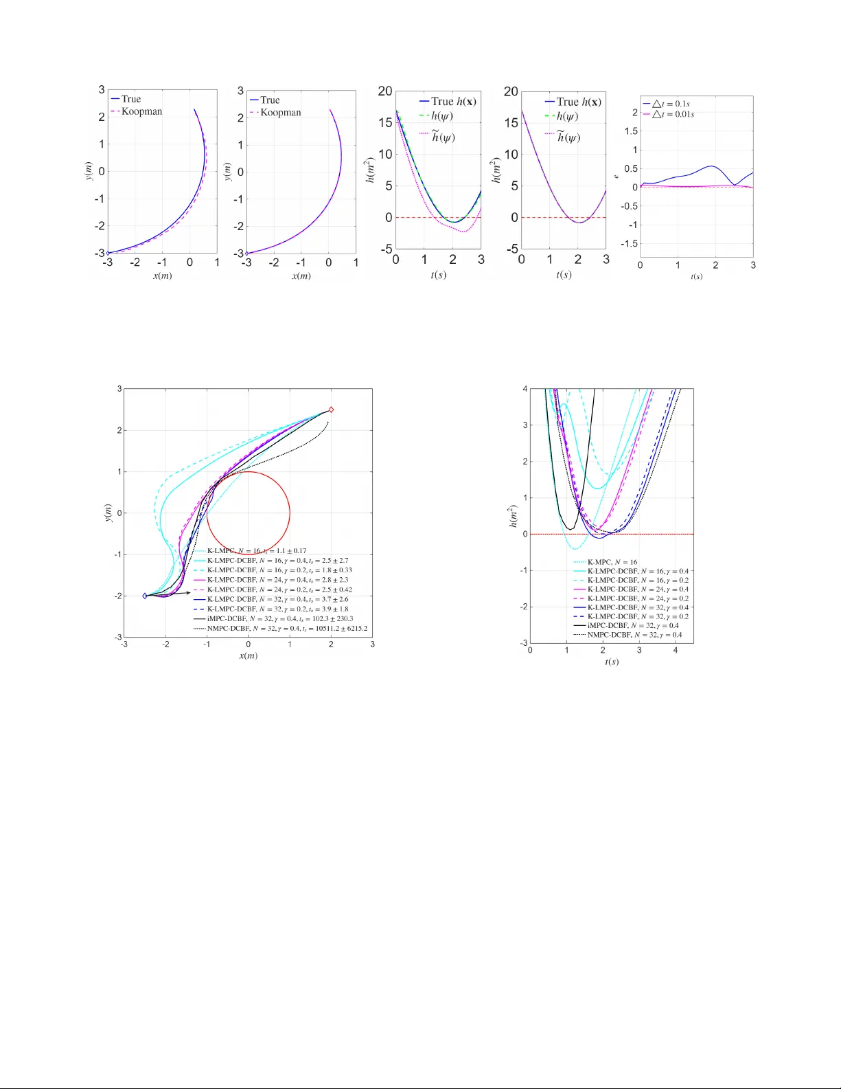
1 K oopman Meets Discr ete-Time Contr ol Barrier Functions: A Linear Model Pr edictive Contr ol Framew ork Shuo Liu 1 , ∗ , Liang W u 2 , ∗ , Dawei Zhang 1 , Jan Drgona 2 and Calin. A. Belta 3 Abstract —This paper proposes a Koopman-based linear model predicti ve control (LMPC) framework for safety-critical control of nonlinear discrete-time systems. Existing MPC formulations based on discrete-time control barrier functions (DCBFs) enfor ce safety thr ough barrier constraints b ut typically r esult in compu- tationally demanding nonlinear programming . T o address this challenge, we construct a DCBF-augmented dynamical system and employ Koopman operator theory to lift the nonlinear dynamics into a higher -dimensional space wher e both the system dynamics and the barrier function admit a linear predictor repr esentation. This enables the transformation of the nonlinear safety-constrained MPC pr oblem into a quadratic pr ogram (QP). T o impr ove feasibility while preser ving safety , a r elaxation mechanism with slack variables is introduced for the barrier constraints. The resulting approach combines the modeling capa- bility of K oopman operators with the computational efficiency of QP . Numerical simulations on a na vigation task f or a r obot with nonlinear dynamics demonstrate that the proposed framework achieves safe trajectory generation and efficient real-time contr ol. I . I N T RO D U C T I O N Ensuring safety is a fundamental requirement in many autonomous systems such as autonomous cars, robots, and aerial vehicles. These systems must operate in complex envi- ronments while satisfying safety requirements such as collision av oidance and input limits. Control Barrier Functions (CBFs) [1], [2] have emer ged as an effecti ve tool for enforcing safety requirements in dynamical systems. By constructing a barrier function whose superle vel set defines the safe region, CBFs guarantee forward in variance of the safe set by imposing affine constraints on the control input. Moreover , stabilization and safety can be addressed simultaneously by combining CBFs with Control L yapunov Functions (CLFs) through quadratic programs (QPs). Extensions of this frame work have been de- veloped to handle high-relati ve-degree constraints and adapti ve control scenarios [3]–[7]. F or discrete-time systems, discrete- time CBFs (DCBFs) were introduced in [8]. The aforementioned approaches are, in general, shortsighted and aggressiv e due to the lack of predicting ahead. Model predictiv e control (MPC) with DCBFs [9] addresses safety in This work was supported in part by the NSF under grant IIS-2024606 at Boston Univ ersity and by a Brendan Iribe endowed professorship at the Univ ersity of Maryland. 1 S. Liu and D. Zhang are with the Department of Mechanical Engineering, Boston University , Brookline, MA, USA { liushuo, dwzhang } @bu.edu 2 L. W u and J. Drgona are with the Department of Civil and Systems En- gineering, Johns Hopkins University , Baltimore, MD, USA { wliang14, jdrgona1 } @jh.edu 3 C. Belta is with the Department of Electrical and Computer Engineering and with the Department of Computer Science, Uni versity of Maryland, College Park, MD, USA cbelta@umd.edu ∗ These authors contributed equally to this work. the discrete-time domain and produces smooth control actions by incorporating future state information over a receding horizon. Howe ver , the computational cost gro ws significantly with the horizon length, as the resulting optimization is typically nonlinear and nonconv ex. T o improv e efficiency and handle high relative-de gree constraints, discrete-time high- order CBFs (DHOCBFs) were introduced within an iterative MPC framew ork [10]. Howe ver , the framew ork still requires successiv e linearizations of the nonlinear dynamics and CBF constraints, and the conv ergence of the resulting iterations is not always guaranteed. An alternative approach is provided by the Koopman op- erator frame work [11], [12], which represents nonlinear dy- namics as linear systems in a lifted state space. Data-driven methods such as Dynamic Mode Decomposition (DMD) and extended DMD (EDMD) enable efficient finite-dimensional approximations of the K oopman operator [13], [14]. Recently , K oopman-based methods have also been explored in CBF- based safety control. For example, [15] lev erages K oopman operators to propagate nonlinear dynamics for efficient safety set computation, [16] learns K oopman-based dynamics and corresponding CBFs for unknown nonlinear systems using neural networks, and [17] develops a K oopman-based identifi- cation scheme with fixed-time con ver gence for safe control of uncertain nonlinear systems. Despite these advances, existing K oopman-CBF approaches do not incorporate prediction over a receding horizon. Integrating Koopman models with MPC enables such prediction capability [18]. Howe ver , to maintain con ve xity in the resulting optimization problem, the CBF constraints still require additional linearization. In this paper , we propose a K oopman-based MPC-DCBF framew ork that enables computationally ef ficient safety- critical control for nonlinear systems. T o the best of our knowledge, this work is the first to inte grate K oopman-based modeling, MPC prediction, and CBF safety constraints within a unified MPC framework. In particular , the contributions are as follows: • W e propose a K oopman-based MPC-DCBF framework for safety-critical control of nonlinear systems by lifting a DCBF-augmented dynamical system into a higher- dimensional linear predictor representation, leading to a linear MPC formulation that can be efficiently solved as a con vex quadratic program. • W e introduce a relaxation mechanism with slack v ariables for the DCBF constraints, which preserves safety guar - antees while improving feasibility and maintaining the quadratic programming structure of the MPC problem. • Numerical simulations on a nonlinear mobile robot nav- igation task demonstrate that the proposed approach achiev es safe trajectory generation while significantly 2 reducing computational cost compared with existing NMPC-DCBF and iterative MPC-DCBF methods. The remainder of the article is organized as follows. In Sec. II, we provide definitions and preliminaries. W e formulate the problem and outline our approach in Sec. III. The proposed K oopman-based MPC-DCBF framew ork is introduced in Sec. IV followed by simulations in Sec. V. W e conclude the paper and discuss directions for future work in Sec. VI. I I . P R E L I M I NA R I E S A. Koopman Operator The authors of [19], [20] introduced an operator -theoretic framew ork for nonlinear dynamical systems. In particular , for the uncontrolled discrete-time system x t +1 = f ( x t ) , K oopman showed that the ev olution of observable functions ψ ( x ) in a Hilbert space can be described by an infinite- dimensional linear operator K defined as K ψ ( x t ) : = ψ ( f ( x t )) . (1) Since Koopman operator theory was originally dev eloped for autonomous systems, several approaches (see [18], [21], [22]) hav e been proposed to extend it to controlled systems x t +1 = f ( x t , u t ) , (2) where x t ∈ X ⊂ R n is the system state at time step t ∈ N , u t ∈ U ⊂ R q is the control input, and f : R n × R q → R n denotes the system dynamics. T o generalize the Koopman op- erator to (2), we adopt the scheme from [18], which introduces an extended state vector ξ =  x u  , (3) where u : = { u k } ∞ k =0 ∈ ℓ ( U ) , with u k ∈ U denoting the k -th element of the control input sequence, and ℓ ( U ) representing the space of all control input sequences. The dynamics of the extended state ξ are described as f ξ ( ξ ) =  f ( x , u 0 ) S u  , (4) where S denotes the left shift operator defined by ( S u ) k : = u k +1 . The Koopman operator associated with the dynamics of the extended state can then be defined on the space of observables ϕ ( ξ ) as K ϕ ( ξ ) : = ϕ ( f ξ ( ξ )) . (5) The infinite-dimensional K oopman operator must be approxi- mated in practice by a finite-dimensional representation. Sev- eral approaches have been proposed to obtain such approxima- tions (see, e.g., [14], [18], [21]), among which the data-driv en Extended Dynamic Mode Decomposition (EDMD) is widely used. In EDMD, the set of observ ables is constructed through a “lifted” mapping ϕ ( x , u ) =  ψ ( x ) u 0  , (6) where ψ ( x ) : =  ψ 1 ( x ) , · · · , ψ n ψ ( x )  ⊤ , n ψ is the designed number of observables (with n ψ ≫ n ), and u 0 denotes the first element of the sequence u . B. Extended Dynamic Mode Decomposition In EDMD, the nonlinear observables ϕ ( x , u ) are expanded using a predefined set of basis functions, such as the Radial Basis Functions used in [18]. The K oopman operator is then identified via an optimization procedure. Specifically , the identification of the approximate K oopman operator reduces to a least-squares problem, assuming that the sampled data { ( x j , u j ) , ( x j + , u j + ) } N d j =1 are collected according to the update mapping  x j + u j +  =  f ( x j , u j 0 ) S u j  , (7) where the subscript + denotes the value at the next time step. The approximate Koopman operator A is then obtained by solving J ( A ) = min A N d X j =1 ∥ ϕ ( x j + , u j + ) − A ϕ ( x j , u j ) ∥ 2 . (8) Since future control inputs do not need to be predicted, the last q rows of A can be removed. Let ¯ A denote the remaining part of A after removing the ro ws associated with the future control input. The matrix ¯ A can then be decomposed as ¯ A = [ A B ] , where A ∈ R n ψ × n ψ and B ∈ R n ψ × q . The problem (8) can be reduced to J ( A, B ) = min A,B N d X j =1 ∥ ψ ( x j + ) − Aψ ( x j ) − B u j 0 ∥ 2 . (9) W e finally obtain the identified linear predictor model in the “lifted” space as ψ k +1 = Aψ k + B u k , (10) where ψ k : = ψ ( x k ) ∈ R n ψ denotes the lifted state. Addition- ally , the output matrix C ∈ R n × n ψ is obtained as the best projection of x onto the span of ψ in a least-squares sense, i.e., as the solution to J ( C ) = min C N d X j =1 ∥ x j − C ψ ( x j ) ∥ 2 . (11) At the end, a linear model for x can be formulated using x k = C ψ k . (12) Remark 1. As [18] claims, if the designed lifted mapping ψ ( x ) contains the state x after the r e-or dering ψ ( x ) ← [ x ⊤ , ψ ( x )] ⊤ , (13) then the solution to (11) is C = [ I , 0] . C. Discrete-T ime Contr ol Barrier Functions (DCBFs) W e consider a discrete-time control system (2) where func- tion f : R n × R q → R n is assumed to be locally Lipschitz continuous. Safety is defined in terms of forward in variance of a set C . Specifically , system (2) is considered safe if, for any initial condition x 0 ∈ C , the state satisfies x t ∈ C for all t ∈ N . W e define C as the superlev el set of a continuous function h : R n → R : C : = { x ∈ R n : h ( x ) ≥ 0 } . (14) 3 Definition 1 (DCBF [23]) . Let C be defined by (14) . A continuous function h : R n → R is a Discrete-time Contr ol Barrier Function (DCBF) for system (2) if there exist class κ function α satisfying α ( r ) < r for all r > 0 such that ∆ h ( x t , u t ) ≥ − α ( h ( x t )) , ∀ x t ∈ C . (15) wher e ∆ h ( x t , u t ) = h ( x t +1 , u t ) − h ( x t ) , and r is the ar gument of α . Theorem 1 (Safety Guarantee [23]) . Given a DCBF h ( x ) fr om Def. 1 with the corresponding set C defined by (14) , if x 0 ∈ C then any Lipschitz contr oller u t that satisfies the constraint in (15) , ∀ t ≥ 0 r enders C forward invariant for system (2) , i.e., x t ∈ C , ∀ t ≥ 0 . W e can simply define a DCBF h ( x ) in (15) satisfying ∆ h ( x t , u t ) ≥ − γ h ( x t ) . (16) where α ( · ) is defined linear and 0 < γ ≤ 1 . Rewrite (16), we have h ( x t +1 , u t ) ≥ (1 − γ ) h ( x t ) . This shows the lower bound of h decreases exponentially with the rate 1 − γ , , and the DCBF turns into the discrete-time exponential CBF [8]. I I I . P RO B L E M F O R M U L A T I O N A N D A P P R OAC H Our objectiv e is to design a closed-loop control strategy for system (2) over the time interval [0 , T ] that minimizes the deviation from a reference state while satisfying safety requirements and state and input constraints. Safety Requirement: System (2) should always satisfy a safety requirement of the form: h ( x t ) ≥ 0 , x t ∈ R n , 0 ≤ t ≤ T , (17) where h : R n → R . Control and State Limitation Requirements: The con- troller u t and state x t must satisfy the state and input constraints x t ∈ X ⊂ R n , u t ∈ U ⊂ R q for 0 ≤ t ≤ T . Objective: W e consider the follo wing cost: J ( u t + k , x t + k ) = N X k =0 ( x t + k − x e ) ⊤ ( x t + k − x e )+ N − 1 X k =0 u ⊤ t + k u t + k , (18) ov er a receding horizon N < T , where x t + k and u t + k denote the predicted state and input at time t + k generated at the current time t , with 0 ≤ t ≤ T . W e define x t +0 = x t and u t +0 = u t , and denote the reference state by x e . A control policy is said to be feasible if all constraints enforcing the aforementioned requirements are mutually non- conflicting for all 0 ≤ t ≤ T . In this paper , we consider the following problem: Problem 1. F ind a feasible control policy for system (2) such that the safety requir ement, contr ol and state limitations are satisfied, and the cost (18) is minimized. T o enforce safety , the authors of [9] incorporated the DCBF constraint h ( x t + k +1 , u t + k ) ≥ ω t + k (1 − γ ) h ( x t + k ) , 0 < γ ≤ 1 (19) into the MPC formulation, where ω t + k ≥ 0 is a relaxation variable introduced to improv e both feasibility and safety . In addition, the system dynamics in (2) and the state and input constraints are included as constraints in the MPC problem to enforce additional requirements. Ho wev er , since both (2) and (19) are generally nonlinear , the resulting optimization prob- lem becomes noncon vex. This approach, commonly referred to as NMPC-DCBF , may lead to high computational cost, particularly when long prediction horizons are considered. T o transform the optimization problem into a con ve x one, the authors of [10] linearize both the system dynamics (2) and the DCBF constraint (19) as linear constraints within an MPC framework. The resulting linear MPC problem is solved iterativ ely at each time step to reduce the linearization error . Howe ver , the con vergence of this iterativ e procedure is not guaranteed. T o address this issue, we propose a Koopman- based MPC-DCBF frame work to construct a linear MPC formulation without requiring iterative linearization. Appr oach: The key idea of this paper is to transform the nonlinear safety-constrained MPC problem into a linear MPC formulation using a K oopman-based lifted representa- tion. First, we augment the original system dynamics with the barrier function to construct a DCBF-augmented dynamical system that explicitly incorporates the safety constraint into the system state. Second, the augmented nonlinear system is lifted into a higher-dimensional space through the K oopman operator framew ork, where the lifted dynamics can be approximated by a linear predictor identified from data. This lifted representa- tion enables both the system dynamics and the barrier function to admit linear expressions in the lifted state. T o improve feasibility while preserving safety guarantees, a relaxation mechanism is introduced for the linearized DCBF constraints. Finally , the resulting lifted linear model is integrated into an MPC formulation together with linearized DCBF constraints, which leads to a linear MPC problem that can be formulated as a conv ex quadratic program and solved efficiently at each control step. I V . K O O P M A N - BA S E D M P C - D C B F F R A M E W O R K In this section, we present the proposed Koopman-based MPC-DCBF frame work, which enables the construction of a con ve x MPC problem for safety-critical systems. The frame- work consists of three main steps: constructing a DCBF- augmented dynamical system, lifting it to a higher -dimensional linear system via K oopman identification, and integrating the resulting lifted model into an MPC formulation. A. DCBF-augmented Dynamic System If only lifting the system (2) to a higher and linear dimension, the Problem 1 usually can not be transformed into a QP because of the existence of the nonlinear and possibly nonconv ex safety constraint (17). Even if h is ℓ 2 - norm DCBF , applying the DCBF constraint (17) to MPC results in a quadratically constrained QP (QCQP), which is computationally hea vier than QP in practice. Moreov er , solving a QP not only has the same O ( n 3 ) time complexity as solving a linear system of equations in theory [24] but also 4 offers data-independent e xecution time certificates [25], [26], which is critical for real-time control applications. T o handle the general nonconv ex DCBF constraint while maintaining computational efficienc y , we incorporate the DCBF h ( x ) as an additional state variable. Consider the discrete-time system (2), where h ( x ) denotes a DCBF en- coding the safety constraint. The augmented state is defined as ¯ x t : =  x t h ( x t )  ∈ R n +1 , (20) which is gov erned by the following DCBF-augmented dy- namic system ¯ x t +1 = ¯ f ( ¯ x t , u t ) : =  f ( x t , u t ) h ( f ( x t , u t ))  . (21) Our idea is to apply the K oopman operator to lift the DCBF- augmented dynamical system (21) into a linear system in a higher-dimensional space. This lifted representation enables both the system dynamics and the DCBF constraint to be expressed linearly in the lifted space, allowing the resulting MPC formulation to be cast as a QP . B. Koopman Identification via Least Squar es T o obtain a linear representation of the nonlinear DCBF- augmented system (21), we employ the Koopman operator framew ork (EDMD in Sec. II-B). The K oopman operator lifts the nonlinear system into a higher-dimensional space of observables where the dynamics can be approximated linearly . Let ψ ( ¯ x ) denote a vector of observable functions of the augmented state ¯ x . The lifted state is defined as ψ t : = ψ ( ¯ x t ) ∈ R n ψ , (22) where n ψ is the dimension of the lifted space. Under the K oopman frame work, the dynamics of the lifted state can be approximated by a linear system ψ t +1 = Aψ t + B u t , (23) where A ∈ R n ψ × n ψ and B ∈ R n ψ × q are constant matrices to be identified. T o compute A and B , we collect data samples { ( ¯ x j , u j , ¯ x j + ) } N d j =1 from the DCBF-augmented system (21), where ¯ x j is the current augmented state and ¯ x j + is the corresponding next-step state. The corresponding lifted data are ψ j = ψ ( ¯ x j ) , ψ j + = ψ ( ¯ x j + ) . Stacking the data ov er N d samples yields Ψ + = A Ψ + B U, (24) where Ψ = [ ψ 1 , . . . , ψ N d ] , Ψ + = [ ψ 1 + , . . . , ψ N d + ] , U = [ u 1 , . . . , u N d ] . The matrices A and B are obtained by solving the following regularized least-squares problem min A,B ∥ Ψ + − A Ψ − B U ∥ 2 F + λ ∥ [ A B ] ∥ 2 F , (25) where λ > 0 is a regularization parameter and ∥ · ∥ F denotes the Frobenius norm. This leads to the closed-form solution [ A B ] = Ψ + V ⊤ ( V V ⊤ + λI ) − 1 , (26) where V = [Ψ ⊤ U ⊤ ] ⊤ . The regularization term improves numerical stability and alleviates potential ill-conditioning of the data matrix. Based on Eqs. (11)–(12), the optimal matrix C admits the closed-form solution C = ¯ X Ψ ⊤ (ΨΨ ⊤ ) − 1 , (27) where ¯ X = [ ¯ x 1 , . . . , ¯ x N d ] . The resulting lifted linear model will be used in the next subsection to construct a linear MPC formulation. C. Koopman-based Linear MPC F ormulation From Sec. IV -B, the lifted linear dynamics obtained via the K oopman framework are given by Eq. (23). Since the augmented state is defined by (20), the barrier value h ( x t ) corresponds to the last component of ¯ x t . Using the identified linear output map (12), (22) and (27), the barrier function can be expressed in the lifted space as h ( x t ) = e ⊤ h ¯ x t = e ⊤ h C ψ t : = ˜ h ( ψ t ) , (28) where e h is the canonical basis vector selecting the last entry of ¯ x t . Therefore, the barrier function is linear in the lifted state. The linear DCBF constraint defined by ˜ h ( ψ t ) can be formu- lated as a linear constraint to enforce the safety requirement. T ogether with the lifted linear dynamics (23) and the state and control bounds x t ∈ X ⊂ R n and u t ∈ U ⊂ R q , the resulting optimization problem yields a linear MPC-DCBF formulation. Note that the state and control bounds may conflict with the system dynamics and DCBF constraints, which can lead to infeasibility . The authors of [9] employed slack variables (decision variables) for DCBFs that enhance both feasibility and safety as shown in (19). While this method enables the flexible integration of safety requirements as soft constraints within the control frame work, the resulting constraints are nonlinear in the decision variables (see Remark 4). As a result, the optimization problem is generally noncon ve x and inherently computationally intensiv e. T o address this issue, we proposed a new relaxation method that can generate linear DCBF constraint. Consider a relaxed DCBF at current step t as ˜ h ( ψ t +1 ) ≥ ω t (1 − γ ) ˜ h ( ψ t ) , (29) where ω t ≥ 0 is a slack variable. Since ˜ h ( ψ t ) depends only on the current lifted state ψ t , which is kno wn at time t , it is treated as a known constant. W e reformulate the DCBF constraint for next step and position a slack variable in front of ˜ h ( ψ t ) as: ˜ h ( ψ t +2 ) ≥ ω t +1 (1 − γ ) 2 ˜ h ( ψ t ) , ω t +1 ≥ 0 , (30) which is a linear constraint in terms of ψ t +2 and ω t +1 . Having established the linearized DCBF , we proceed to link its construction to open-loop safety via the following theorem. Theorem 2. Given a linearized DCBF ˜ h ( ψ ) for sys- tem (23) , if ˜ h ( ψ t ) ≥ 0 , then any Lipschitz contr ollers u t , ..., u t + N − 1 that satisfy the constraints ˜ h ( ψ t + k +1 ) ≥ ω t + k (1 − γ ) k +1 ˜ h ( ψ t ) , 0 < γ ≤ 1 , ω t + k ≥ 0 , k ∈ { 0 , ..., N − 1 } r ender ˜ h ( ψ t + k +1 ) ≥ 0 . 5 Pr oof. Since ˜ h ( ψ t ) ≥ 0 , 1 − γ ≥ 0 , ω t ≥ 0 , we hav e ˜ h ( ψ t +1 ) ≥ ω t (1 − γ ) ˜ h ( ψ t ) ≥ 0 . Since ˜ h ( ψ t +1 ) ≥ 0 , (1 − γ ) 2 ≥ 0 , ω t +1 ≥ 0 , we hav e ˜ h ( ψ t +2 ) ≥ ω t +1 (1 − γ ) 2 ˜ h ( ψ t +1 ) ≥ 0 . Repeatedly we have ˜ h ( ψ t + k +1 ) ≥ 0 , k ∈ { 0 , ..., N − 1 } . From the above proof, we observe that although a slack variable ω t + k is introduced into the constraint, the open- loop safety (i.e., ˜ h ( ψ t + k +1 ) ≥ 0 , k ∈ { 0 , ..., N − 1 } ) is still guaranteed. Moreover , when no control input satisfies ˜ h ( ψ t + k +1 ) ≥ ω t + k (1 − γ ) k +1 ˜ h ( ψ t ) , the slack variable ω t + k can be reduced to a v alue in the range ω t + k ∈ [0 , 1) , thereby relaxing the right-hand side of the constraint to improv e feasibility . This relaxation method enables us to incorporate DCBF constraints in a linear MPC (LMPC) formulation: LMPC-DCBF: min U t , Ψ t , Ω t p ( ψ t + N ) + N − 1 X k =0 q ( ψ t + k , u t + k , ω t + k ) (31a) s.t. ψ t + k +1 = Aψ t + k + B u t + k , k = 0 , . . . , N − 1 , (31b) E x C ψ t + k ∈ X , k = 1 , . . . , N , (31c) u t + k ∈ U , k = 0 , . . . , N − 1 , (31d) ˜ h ( ψ t + k +1 ) ≥ ω t + k (1 − γ ) k +1 ˜ h ( ψ t ) , 0 < γ ≤ 1 , (31e) ω t + k ≥ 0 , k = 0 , . . . , N − 1 , (31f) where U t = [ u t , . . . , u t + N − 1 ] , Ψ t = [ ψ t , . . . , ψ t + N ] and Ω t = [ ω t , . . . , ω t + N − 1 ] . E x = [ I n 0 ] is a selection matrix that extracts the original state x t from the augmented state ¯ x t . Thus, ψ t + k in the cost function (31a) can be con verted to x t + k = E x C ψ t + k , enabling the cost to penalize the deviation from the desired state x e in (18). In practice, ω t + k is treated as an optimization variable that is penalized tow ard 1—either through a large weight in the cost function or via a lexicographic priority . As a result, when the hard DCBF constraint is feasible, the optimizer yields ω ⋆ t + k ≈ 1 (i.e., no relaxation). Otherwise, it computes a minimally relaxed solution that still ensures ˜ h ( ψ t + k +1 ) ≥ 0 . Remark 2. Based on [10, Def. 1], if ˜ h ( ψ t ) has r elative degr ee m and the constr aints in an optimal contr ol pr oblem consist solely of DCBF constraints (31e) , then the DCBFs must be formulated up to the m th or der to ensure that the contr ol input u t appears explicitly , i.e., the control input u t will appears in ˜ h ( ψ t + m , u t ) . Howe ver , if the framework also includes the system dynamics (31b) as constraints—wher e u t is already explicitly r epresented—then the or der of the DCBFs can be chosen more flexibly to r educe computational comple xity . In particular , if m ≤ N , the DCBF order can be set to 1, since the contr ol input will af fect the DCBF constr aints within the pr ediction horizon. In our LMPC-DCBF frame work (31) , since the barrier function is repr esented in the lifted space by (28) , its relative de gree with respect to the lifted linear system (31b) is determined by the smallest inte ger m such that e ⊤ h C A m − 1 B  = 0 , (32) while e ⊤ h C A i B = 0 , i = 0 , . . . , m − 2 . Thus, when identifying A , B , and C in (26) – (27) , the r elative de gree m of the barrier function with r espect to the lifted system cannot be pr edetermined while pr eserving the accuracy of the lifted dynamics. Ther efore , the pr ediction horizon N should be chosen sufficiently larg e to ensur e m ≤ N . Remark 3. The Koopman-based lifted model in (31b) is obtained fr om a finite-dimensional appr oximation of the Koop- man operator using data-driven identification. As a r esult, the lifted linear dynamics only approximate the original nonlinear system and modeling err ors may exist. Therefor e, the safety guarantees derived fr om the linear MPC-DCBF formulation cannot strictly ensure safety of the original nonlinear system in a rigor ous sense. In practice, this issue can be mitigated thr ough several conservative design choices. F or example, a safety mar gin can be incorporated into the barrier func- tion, i.e., enforcing ˜ h ( ψ t ) ≥ ϵ with ϵ > 0 , to compensate for approximation err ors. In addition, the class κ function hyperparameter γ in the DCBF constraint can be adjusted. Choosing a smaller γ leads to mor e conservative constraints and str engthens the safety enforcement. In this paper , we adopt the latter strate gy and re gulate the safety level by tuning γ , as illustrated in the numerical examples in Sec. V. Remark 4. In [9], the r elaxation technique places the slac k variable ω t + k in fr ont of (1 − γ ) h ( x t + k ) , yielding h ( x t + k +1 , u t + k ) ≥ ω t + k (1 − γ ) h ( x t + k ) , ω t + k ≥ 0 . (33) However , ω t + k is a decision variable, and x t + k is also a decision variable for k ≥ 1 in the MPC pr oblem. As a r esult, the pr oduct ω t + k h ( x t + k ) intr oduces a nonlinear constraint, which leads to a noncon vex optimization pr oblem. T o addr ess this issue, in Theor em 2 we establish a r ecursive r elationship that connects the futur e barrier values ˜ h ( ψ t + k +1 ) to the known constant ˜ h ( ψ t ) . By multiplying the slack variable ω t + k with this known quantity , we obtain the constraint in (31e) , which is linear with respect to the decision variables. D. Complexity Analysis All constraints in (31b)–(31e) are af fine in the decision variables. As a result, the resulting optimization problem is a con vex QP at each time step. The decision variables consist of the predicted control inputs U t = [ u t , . . . , u t + N − 1 ] , lifted states Ψ t = [ ψ t , . . . , ψ t + N ] , and relaxation variables Ω t = [ ω t , . . . , ω t + N − 1 ] . Since the lifted state dimension n ψ , the input dimension q , and the prediction horizon N have been defined previously , the number of decision variables in the LMPC-DCBF problem (31) scales on the order of O ( N ( n ψ + q )) . Here we omit the contribution of the re- laxation variables ω t + k since each of them is scalar and thus does not af fect the asymptotic complexity order . Using standard interior-point methods, the worst-case computational complexity scales as O  ( N ( n ψ + q )) 3  . In practice, structure- exploiting QP solvers (e.g., OSQP) typically achiev e signifi- cantly faster performance. Compared with [9], [10], the proposed K oopman-based LMPC-DCBF frame work maintains a con vex QP structure and a voids iterative linearization steps within each control update, which substantially reduces the computational burden and facilitates real-time implementation. 6 V . N U M E R I C A L E X A M P L E S In this section, we present numerical results to validate our proposed approach using a unicycle model. W e compare the performance of the proposed method with the baseline NMPC-DCBF and iMPC-DCBF approaches. For the proposed method, the QP problem were solv ed using quadprog . For iMPC-DCBF , OSQP [27] was used to solve the con vex opti- mization problem at each iteration. NMPC-DCBF was solved using IPOPT [28] with the modeling language Y ALMIP [29]. All simulations were conducted on a W indows desktop with an Intel® Core™ i7-11750F CPU @ 2.50 GHz. A. System Dynamics and DCBF Consider a continuous-time unicycle model in the form     ˙ x ( t ) ˙ y ( t ) ˙ θ ( t ) ˙ v ( t )     =     v ( t ) cos ( θ ( t )) v ( t ) sin ( θ ( t )) 0 0     +     0 0 0 0 1 0 0 1      u 1 ( t ) u 2 ( t )  . (34) where x ( t ) = [ x ( t ) , y ( t ) , θ ( t ) , v ( t )] ⊤ captures the 2-D loca- tion, heading angle, and linear speed; u ( t ) = [ u 1 ( t ) , u 2 ( t )] ⊤ represents angular velocity ( u 1 ) and linear acceleration ( u 2 ), respectiv ely . The discrete-time model used in this paper is obtained by discretizing (34) using a standard fourth-order Runge–Kutta scheme with sampling time ∆ t , yielding the discrete-time model in (2). As a candidate DCBF function h ( x t ) , we choose a quadratic distance function for circular obstacle avoidance h ( x t ) = ( x t − x 0 ) 2 + ( y t − y 0 ) 2 − r 2 , where ( x 0 , y 0 ) and r denote the obstacle center location and radius, respectiv ely . In this work, we set x 0 = 0 , y 0 = 0 , and r = 1 . B. Koopman Identification T o identify the lifted linear predictor , we generate state- transition data ( x t , u t , x t +1 ) using the discrete-time model. Random initial states and control inputs are sampled within the admissible ranges to construct the dataset used for regression. T o handle the periodicity of the heading angle, the lifted state does not directly include θ t . Instead, we use the trigonometric coordinates (sin θ t , cos θ t ) . The lifted state includes the physi- cal states [ x t , y t , v t , sin θ t , cos θ t ] ⊤ , the dynamics-consistent terms [ v t cos θ t , v t sin θ t ] ⊤ , and the candidate DCBF function h ( x t ) . T o further improve approximation accuracy , Gaussian radial basis functions (RBFs) [14] are included in the lifted space, resulting in the lifted state ψ t . Using the collected dataset and the EDMD formulation introduced in Sec. IV -B, we identify the lifted linear dynamics in (23). The dataset contains N d = 2 × 10 5 transition samples generated from randomly sampled initial states and inputs within the ranges x, y ∈ [ − 3 , 3] , θ ∈ [ − π , π ] , v ∈ [ − 3 , 3] , and u 1 , u 2 ∈ [ − 3 , 3] . The physical states are reconstructed from the leading lifted states, while the heading angle is recovered from (sin θ t , cos θ t ) using atan2 . Fig. 1 illustrates the prediction performance of the iden- tified Koopman model. The initial state is set to x 0 = [ − 3 , − 3 , 0 , 0 . 2] ⊤ . T o distinguish it from the true state x t generated by the nonlinear dynamics, we denote by ˆ x t the state reconstructed from the K oopman predictor . Figs. 1a – 1b show the trajectories obtained from the true system and the K oopman model under sampling times ∆ t = 0 . 1 s and ∆ t = 0 . 01 s, respecti vely . Figs. 1c – 1d compare the obstacle function values, where h ( x t ) denotes the true barrier function ev aluated at the true state (nonlinear), h ( ψ t ) is computed using the reconstructed K oopman state (nonlinear), and ˜ h ( ψ t ) is obtained directly from the lifted state (linear). Fig. 1e shows the prediction error e t = ∥ x t − E x C ψ t ∥ 2 . It can be observed that the K oopman predictor closely matches the true system behavior , and the approximation accuracy improves as the sampling time ∆ t decreases. C. MPC Design The cost function of the MPC problem consists of stage cost q ( ψ t + k , u t + k , ω t + k ) = P N − 1 k =0 ( || ψ t + k − ψ r || 2 Q + || u t + k − u r || 2 R + || ω t + k − ω r || 2 S ) and terminal cost p ( ψ t + N ) = || ψ t + N − ψ r || 2 P , where Q = P = diag (500 , 500 , 80 , 80 , 10) , R = diag(0 . 3 , 0 . 5) and S = 1000 . x 0 = [ − 2 . 5 , − 2 , 0 . 2 , 2] ⊤ . x e = E x C ψ r = [2 , 2 . 5 , 0 , 0 . 3] ⊤ . The other references are u r = [0 , 0] T and ω r = 1 . The system (34) is discretized with ∆ t = 0 . 01 and is subject to the following state and input constraints: X = { x t ∈ R 4 : − 3 · I 4 × 1 ≤ x t ≤ 3 · I 4 × 1 } , U = { u t ∈ R 2 : − 3 · I 2 × 1 ≤ u t ≤ 3 · I 2 × 1 } . (35) W e incorporate the K oopman model identified in Sec- tion V -B into the MPC framework to solve the optimization problem in (31). The resulting controller is referred to as K-LMPC-DCBF . If the DCBF constraint (31e) is removed from the optimization, the controller reduces to K-LMPC. As benchmarks, we compare with iMPC-DCBF [10], where the maximum iteration number is set to j max = 1000 , and NMPC- DCBF [9]. T o ensure a fair comparison, the parameters of all methods are kept identical. As shown in Fig. 2, without the DCBF constraint, K-LMPC enters the obstacle region and therefore violates safety . In contrast, K-LMPC-DCBF is able to enforce safety during the motion. It can also be observed that as the prediction horizon N increases, the trajectory of K-LMPC-DCBF approaches the obstacle boundary . This occurs because a longer prediction horizon allows the optimizer to choose a more path-optimal control strategy . For the case N = 32 and γ = 0 . 4 , K-LMPC-DCBF slightly penetrates the obstacle region. This is because the controller attempts to optimize the path while the K oopman-lifted dy- namics and DCBF constraints are only approximations of the true system, which introduces modeling errors. Ho wev er , when γ is reduced to 0 . 2 , a more conserv ativ e DCBF condition is enforced and the trajectory becomes safe again, which is consistent with the analysis in Remark 3. Both iMPC-DCBF and NMPC-DCBF can guarantee safety for the case N = 32 , γ = 0 . 4 . Howe ver , the computa- tional adv antage of K-LMPC-DCBF is significant. The a verage control computation time of K-LMPC-DCBF is about 3 – 5 ms per step, while iMPC-DCBF requires approximately 7 (a) T rajectory , ∆ t = 0 . 1 s (b) Trajectory , ∆ t = 0 . 01 s (c) DCBFs, ∆ t = 0 . 1 s (d) DCBFs, ∆ t = 0 . 01 s (e) Error Fig. 1: Comparison between the true nonlinear dynamics and the identified K oopman predictor . Left: x – y trajectories generated by the true system and the K oopman model. Middle: evolution of the DCBFs. Right: prediction error e t = ∥ x t − ˆ x t ∥ 2 . Fig. 2: Trajectory comparison in the presence of a circular obstacle. The robot mov es from the start (blue diamond) to the goal (red diamond). The black arrow indicates the initial v elocity direction of the robot. T rajectories generated by the proposed K-LMPC-DCBF with different prediction horizons N and hyperparameters γ are compared with iMPC- DCBF and NMPC-DCBF . The legend also reports the av erage computation time per step t s (ms). 100 – 330 ms, which is about 30 – 60 times slower . NMPC- DCBF is the slo west, taking about 10500 – 16700 ms per step (around 3500 times slower). These results demonstrate the substantial computational ef ficiency of the proposed K-LMPC- DCBF framew ork. T o better visualize safety , Fig. 3 shows the DCBF v alue ov er time for all methods. For K-LMPC-DCBF , when γ is fixed, increasing the prediction horizon N decreases the minimum value of h , bringing the trajectory closer to the obstacle boundary . Con versely , for fixed N , a smaller γ results in a larger minimum v alue of h , indicating a more conservati ve and safer behavior . This again demonstrates the safety guarantee Fig. 3: Evolution of the DCBFs under different control strate- gies. The red dashed line indicates the safety boundary . provided by K-LMPC-DCBF . Fig. 4 sho ws the control inputs generated by K-LMPC- DCBF under different hyperparameter settings. The inputs remain within the prescribed bounds throughout the motion, confirming that the control constraints are respected. At the beginning of the maneuv er, relatively large control actions are required to steer the robot away from the obstacle. Some nonsmooth variations can be observed during this stage when the safety constraints become activ e and the inputs approach their bounds, which is typical for constrained MPC-based safety controllers. As the robot moves away from the obstacle and approaches the goal, the control inputs gradually become smoother and conv erge toward zero. V I . C O N C L U S I O N This paper proposed a Koopman-based MPC-DCBF frame- work for safety-critical control of nonlinear discrete-time sys- tems. By incorporating the barrier function into the lifted state 8 (a) N = 16 , γ = 0 . 2 (b) N = 24 , γ = 0 . 2 Fig. 4: Control inputs u 1 and u 2 ov er time for K-LMPC-DCBF under different hyperparameter settings. and identifying a linear predictor using K oopman operator theory , the nonlinear safety-constrained MPC problem can be transformed into a con ve x quadratic program. This formulation enables efficient real-time computation while preserving safety guarantees through DCBF constraints. Numerical simulations on a mobile robot navigation task demonstrated that the proposed method achiev es safe trajec- tory generation and significantly reduces computational cost compared with NMPC-DCBF and iterati ve MPC-DCBF ap- proaches. Future work will focus on extending the framew ork to more complex environments, addressing model uncertainty , and applying the method to hardware experiments and multi- agent systems. R E F E R E N C E S [1] A. D. Ames, J. W . Grizzle, and P . T abuada, “Control barrier function based quadratic programs with application to adaptive cruise control, ” in 53rd IEEE conference on decision and control . IEEE, 2014, pp. 6271–6278. [2] A. D. Ames, X. Xu, J. W . Grizzle, and P . T abuada, “Control barrier function based quadratic programs for safety critical systems, ” IEEE T ransactions on Automatic Contr ol , vol. 62, no. 8, pp. 3861–3876, 2016. [3] Q. Nguyen and K. Sreenath, “Exponential control barrier functions for enforcing high relativ e-degree safety-critical constraints, ” in 2016 American Control Conference (ACC) , 2016, pp. 322–328. [4] W . Xiao and C. Belta, “High-order control barrier functions, ” IEEE T ransactions on Automatic Contr ol , vol. 67, no. 7, pp. 3655–3662, 2021. [5] W . Xiao, C. Belta, and C. G. Cassandras, “ Adaptiv e control barrier functions, ” IEEE Tr ansactions on Automatic Contr ol , vol. 67, no. 5, pp. 2267–2281, 2021. [6] S. Liu, W . Xiao, and C. A. Belta, “ Auxiliary-variable adaptive control barrier functions for safety critical systems, ” in 2023 62th IEEE Con- fer ence on Decision and Control (CDC) , 2023. [7] ——, “ Auxiliary-variable adaptiv e control lyapunov barrier functions for spatio-temporally constrained safety-critical applications, ” in 2024 IEEE 63r d Conference on Decision and Contr ol (CDC) , 2024, pp. 8098–8104. [8] A. Agrawal and K. Sreenath, “Discrete control barrier functions for safety-critical control of discrete systems with application to bipedal robot navigation. ” in Robotics: Science and Systems , vol. 13. Cam- bridge, MA, USA, 2017, pp. 1–10. [9] J. Zeng, Z. Li, and K. Sreenath, “Enhancing feasibility and safety of nonlinear model predictive control with discrete-time control barrier functions, ” in 2021 60th IEEE Conference on Decision and Control (CDC) , 2021, pp. 6137–6144. [10] S. Liu, J. Zeng, K. Sreenath, and C. A. Belta, “Iterative conv ex optimization for model predictive control with discrete-time high-order control barrier functions, ” in 2023 American Control Conference (A CC) , 2023, pp. 3368–3375. [11] C. W . Rowley , I. Mezi ´ c, S. Bagheri, P . Schlatter, and D. S. Henningson, “Spectral analysis of nonlinear flows, ” Journal of fluid mechanics , vol. 641, pp. 115–127, 2009. [12] M. Budi ˇ si ´ c, R. Mohr , and I. Mezi ´ c, “ Applied koopmanism, ” Chaos: An Inter disciplinary Journal of Nonlinear Science , vol. 22, no. 4, 2012. [13] P . J. Schmid, “Dynamic mode decomposition of numerical and experi- mental data, ” Journal of fluid mechanics , vol. 656, pp. 5–28, 2010. [14] M. Williams, I. Kevrekidis, and C. Rowle y , “ A data-driven approxima- tion of the Koopman operator: Extending dynamic mode decomposi- tion, ” Journal of Nonlinear Science , vol. 25, pp. 1307–1346, 2015. [15] C. Folkestad, Y . Chen, A. D. Ames, and J. W . Burdick, “Data-driven safety-critical control: Synthesizing control barrier functions with koop- man operators, ” IEEE Control Systems Letters , vol. 5, no. 6, pp. 2012– 2017, 2020. [16] V . Zinage and E. Bakolas, “Neural Koopman control barrier functions for safety-critical control of unknown nonlinear systems, ” in 2023 American Contr ol Confer ence (ACC) , 2023, pp. 3442–3447. [17] M. Black and D. Panagou, “Safe control design for unknown non- linear systems with Koopman-based fixed-time identification, ” IF AC- P apersOnLine , vol. 56, no. 2, pp. 11 369–11 376, 2023. [18] M. Korda and I. Mezi ´ c, “Linear predictors for nonlinear dynamical sys- tems: K oopman operator meets model predictive control, ” Automatica , vol. 93, pp. 149–160, 2018. [19] B. K oopman, “Hamiltonian systems and transformation in Hilbert space, ” Proceedings of the National Academy of Sciences , vol. 17, no. 5, pp. 315–318, 1931. [20] B. Koopman and J. Neumann, “Dynamical systems of continuous spectra, ” Proceedings of the National Academy of Sciences , vol. 18, no. 3, pp. 255–263, 1932. [21] M. Williams, M. Hemati, S. Dawson, I. K evrekidis, and C. Rowley , “Extending data-driven Koopman analysis to actuated systems, ” IF AC- P apersOnLine , vol. 49, no. 18, pp. 704–709, 2016. [22] J. Proctor , S. Brunton, and J. Kutz, “Generalizing Koopman theory to allow for inputs and control, ” SIAM J ournal on Applied Dynamical Systems , vol. 17, no. 1, pp. 909–930, 2018. [23] Y . Xiong, D.-H. Zhai, M. T avakoli, and Y . Xia, “Discrete-time control barrier function: High-order case and adaptive case, ” IEEE Tr ansactions on Cybernetics , pp. 1–9, 2022. [24] L. W u and R. D. Braatz, “ A Quadratic Programming Algorithm with O ( n 3 ) Time Complexity , ” IEEE T ransactions on A utomatic Contr ol , pp. 1–16, 2026. [25] ——, “ A Direct Optimization Algorithm for Input-constrained MPC, ” IEEE T ransactions on Automatic Control , vol. 70, no. 2, pp. 1366–1373, 2025. [26] L. W u, W . Xiao, and R. D. Braatz, “EIQP: Execution-time-certified and Infeasibility-detecting QP Solver , ” IEEE T ransactions on Automatic Contr ol , pp. 1–16, 2025. [27] B. Stellato, G. Banjac, P . Goulart, A. Bemporad, and S. Boyd, “OSQP: An operator splitting solver for quadratic programs, ” Mathematical Pr ogramming Computation , vol. 12, no. 4, pp. 637–672, 2020. [28] L. T . Biegler and V . M. Zav ala, “Large-scale nonlinear programming using IPOPT: An integrating frame work for enterprise-wide dynamic optimization, ” Computers & Chemical Engineering , vol. 33, no. 3, pp. 575–582, 2009. [29] J. Lofberg, “Y ALMIP: A toolbox for modeling and optimization in MA TLAB, ” in 2004 IEEE international confer ence on r obotics and automation (IEEE Cat. No. 04CH37508) , 2004, pp. 284–289.