Predictor-Feedback Stabilization of Linear Switched Systems with State-Dependent Switching and Input Delay

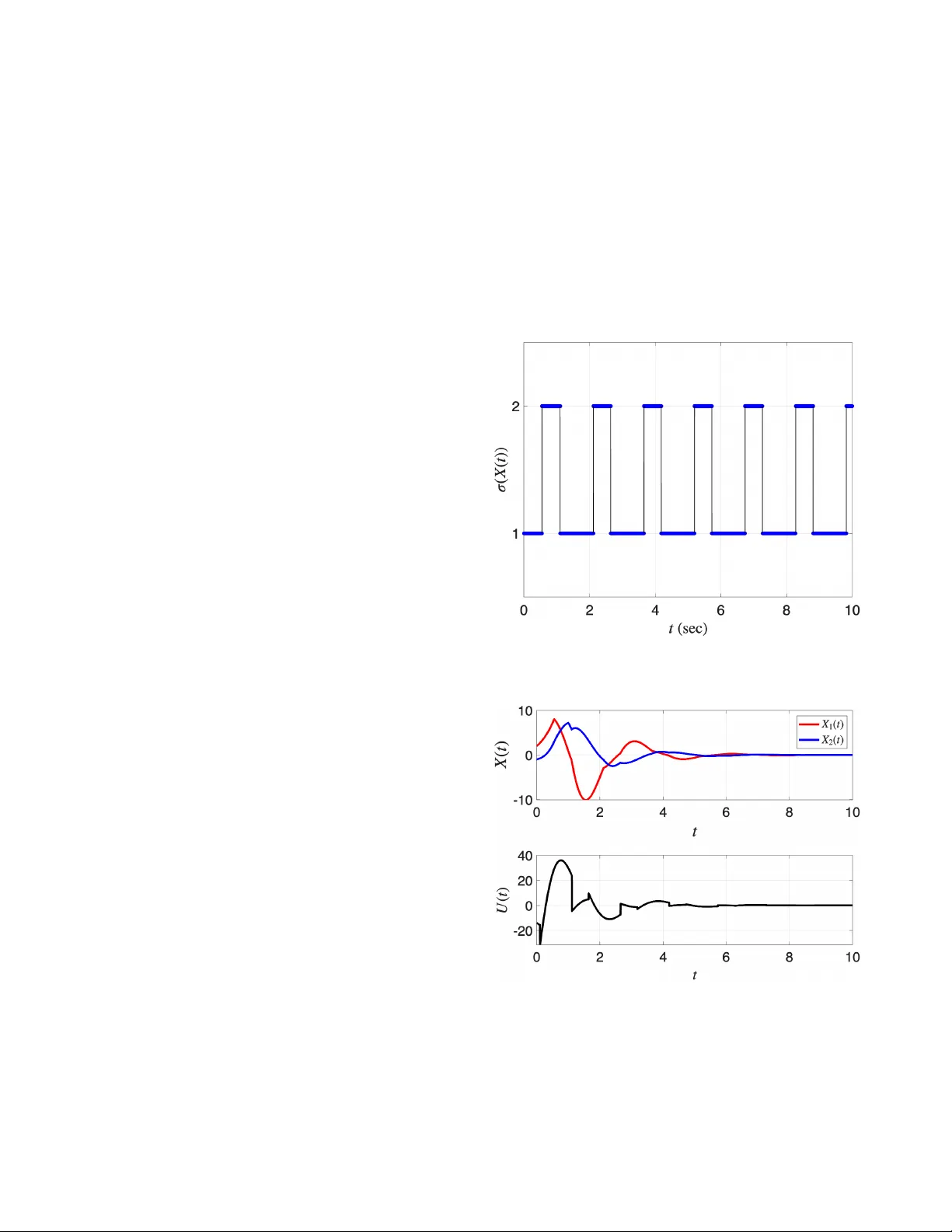
Pr edictor -F eedback Stabilization of Linear Switched Systems with State-Dependent Switching and Input Delay ∗ Andreas Katsanikakis 1 , Nikolaos Bekiaris-Liberis 1 and Delphine Bresch-Pietri 2 Abstract — W e develop a pr edictor-feedback contr ol design for a class of linear systems with state-dependent switching. The main ingredient of our design is a novel construction of an exact predictor state. Such a construction is possible as for a gi ven, state-dependent switching rule, an implementable formula for the predictor state can be derived in a way analogous to the case of nonlinear systems with input delay . W e establish unif orm exponential stability of the corresponding closed-loop system via a novel construction of multiple L yapunov functionals, relying on a backstepping transf ormation that we introduce. W e validate our design in simulation considering a switching rule motivated by communication networks. I . I N T RO D U C T I O N Systems with state-dependent switching and input delay appear in various applications. Among dif ferent potential application examples we discuss the following three. In vehi- cle control, state-dependent switching occurs between throt- tle and braking operations depending on speed/acceleration states, while input delays appear due to engine and other ac- tuator dynamics, see, e.g., [1], [2]. When modeling epidemic spreading dynamics, state-dependent switching may appear due to external measures imposition, such as quarantine measures, implemented depending on, e.g., the number of infected individuals, while at the same time, input delays may arise due to lags between implementation of policy- maker strategies and their effect on epidemic spreading, see, e.g., [3], [4], [5], [6]. In network ed control systems, state- dependent switching originates from communication proto- cols and scheduling rules, while delays appear due to, e.g., communication constraints [7], [8]. These examples high- light the fact that simultaneous presence of state-dependent switching and input delay is common in practice, motiv ating the need for dev elopment of control design methods for this class of systems. The majority of related existing results address either input delays in systems with time-dependent switching, or state delays in systems with state-dependent switching. F or the former case, there exist methods aiming at input delay compensation relying, for example, on construction of Linear ∗ Funded by the European Union (ERC, C-NORA, 101088147). V iews and opinions expressed are ho wev er those of the authors only and do not necessarily reflect those of the European Union or the European Research Council Executiv e Agenc y . Neither the European Union nor the granting authority can be held responsible for them. 1 The authors are with the Department of Electrical and Computer Engineering, T echnical Univ ersity of Crete, Chania, 73100, Greece. Emails: akatsanikakis@tuc.gr and nlimperis@tuc.gr. 2 The author is with MINES ParisT ech, PSL Research University CAS- Centre Automatique et Systemes, 60 Boulev ard Saint Michel 75006, Paris, France. Email: delphine.bresch-pietri@minesparis.psl.eu. Matrix Inequalities (LMIs) [9], [10], [11], [12], [13], [14], [15], [16] and L yapuno v-Krasovski functionals [17], [18], or on the truncated predictor method [19], [20], [21]. Howe ver , in these works the delay length or the system dynamics are typically restricted. Systems with state delays and state- dependent switching, which, in general, require different treatment than the case of input delay , are addressed in [22], [23]. Moreo ver , input delay of arbitrary length is compen- sated developing predictor -based designs in [24], [25], which address systems with switched delays rather than switched dynamics, and in [26], [27] that consider time-dependent switching. Predictor -based control of discrete-time systems when the switching signal itself is the control input are addressed in [28], which, although related, it is a different problem. T o the best of our knowledge, there exists no result addressing the problem of (long) input delay compensation for linear switched systems with state-dependent switching via predictor feedback. In this paper we develop a ne w predictor-feedback control law for a class of linear switched systems with input delay , in which the switching signal depends on the state. For a giv en switching rule, the main element of our predictor - feedback control design is a novel construction of an exact predictor state, which enables complete delay compensation. Differently from our previous works [26], [27], here an exact predictor state construction is possible because, as the switching rule depends on the state, an implicit, im- plementable formula for the predictor state can be deriv ed viewing the given switched system as a nonlinear system. W e thus provide such a predictor state construction and we furthermore deriv e an alternativ e, semi-explicit formula for its computation, capitalizing on the fact that, at each mode, the system dynamics are linear . W e establish uni- form exponential stability of the closed-loop system via construction of multiple L yapunov functionals relying on a backstepping transformation that we introduce. W e v alidate the control design’ s performance in simulation using a two- mode system with a switching rule whose form is motiv ated by communication netw ork applications. The remainder of the paper is organized as follo ws. Section II presents the class of switched systems with input delay considered and the predictor-feedback control design. Section III provides the stability analysis, where the main result is presented. Section IV illustrates the theoretical results through a simulation example. Finally , Section V provides concluding remarks. I I . P RO B L E M F OR M U L AT I O N A N D C O N T RO L D E S I G N A. Switched Linear Systems W ith Input Delay and State- Dependent Switching W e consider the follo wing linear switched system with a constant delay in the input ˙ X ( t ) = A σ ( X ( t )) X ( t ) + B σ ( X ( t )) U ( t − D ) , (1) where X ∈ R n is the state, U ∈ R is the control input, D > 0 is an arbitrarily long delay , and t ≥ 0 is the time variable. The switching signal σ : R n → P maps the state to a finite set of modes P = { 1 , 2 , . . . , p } . The state space is partitioned into a finite collection of disjoint regions { Ω 1 , Ω 2 , . . . , Ω p } such that S p i = 1 Ω i = R n , Ω i ∩ Ω j = ∅ , ∀ i  = j , where each region Ω i corresponds to a distinct mode of the switched system, i.e., σ ( X ) = i if and only if X ∈ Ω i . Furthermore, we define Ω j , i = Ω i , j ⊆ Ω i ∪ Ω j as the switching surfaces between adjacent re gions. W e impose the following assumptions on the delay-free system. The first guarantees well-posedness of both the open- and closed-loop systems and the second implies that the delay-free system can be stabilized by a nominal control law of the form U = K σ X . Assumption 2.1: For any initial condition X 0 ∈ R n and any disturbance d ∈ L 2 loc ([ 0 , ∞ ) ; R ) , the systems ˙ X ( t ) =  A σ ( X ( t )) + B σ ( X ( t )) K σ ( X ( t ))  X ( t ) , (2) ˙ X ( t ) = A σ ( X ( t )) X ( t ) + B σ ( X ( t )) d ( t ) , (3) hav e a unique, absolutely continuous solution, in Carath ´ eodory sense 2 defined on R + . Moreov er , the corresponding switching signal σ ( X ( t )) is piece wise constant and exists for all non-negati ve times (thus it does not exhibit Zeno beha vior). Assumption 2.2: There exist families of vectors K T i , of symmetric matrices P i , Q i , such that Q i > 0, and of positive constants α i , β i , such that the following hold α i | X | 2 ≤ X ⊤ P i X ≤ β i | X | 2 , ∀ X ∈ Ω i , (4) X T h ( A i + B i K i ) T P i + P i ( A i + B i K i ) + Q i i X ≤ 0 , ∀ X ∈ Ω i , (5) X T ( P j − P i ) X = 0 , ∀ X ∈ Ω i j , (6) for all i , j ∈ P . Remark 2.3: Assumption 2.1 guarantees well-posedness of both the open- and closed-loop systems, when employing predictor-feedback, under the giv en state-dependent switch- ing law σ ( X ) . It also e xcludes the possibility of the appear- ance of Zeno behavior . Note that, for the considered partition of the state space, sliding phenomena are also excluded, while chattering phenomena are not. Such phenomena are undesirable for control implementation purposes, but they 2 See, e.g., [29] and references therein, for specific conditions that guarantee this. can be practically avoided via emplo ying hysteresis switch- ing (see e.g., [30], [31]). Moreover , Assumption 2.2 guar- antees that one can construct multiple, quadratic L yapunov functions to study stability of the nominal (in the delay-free case) closed-loop system (2), as in, e.g., [30], [31]. Ho we ver , condition (6) is more restrictive as it imposes continuity at the switching surfaces of the respectiv e L yapunov functions. This is consistent with our setup in which σ depends only on X and where the Ω i sets are such that Ω i , j = Ω j , i , while belonging to some Ω i ( resp. Ω j ) . Both assumptions may be restrictive, nevertheless, they are necessary here, in order to properly define the predictor state and to carry out the stability analysis, without the need to employ a hybrid systems framework. B. Pr edictor-F eedback Contr ol Design And Computation The values of the predictor are the future values of the system state, and since the switching logic is state-dependent, we face a situation analogous to a non-linear system with input delay , where the predictor state formula is implicit, see, for e xample, [32], [33], and [34]. The reason for this is that the system parameters ( A σ , B σ ) depend on the switching mode, which in turn depends on the future state. Hence, the predictor state satisfies an implicit integral equation given by P ( θ ) = X ( t ) + Z θ t − D  A σ ( P ( s )) P ( s ) + B σ ( P ( s )) U ( s )  d s , (7) for t − D ≤ θ ≤ t . Note that this definition is implicit because the switching mode σ ( P ( θ )) depends explicitly on the unknown future predictor state P ( θ ) . Having defined the predictor state P ( t ) , we now propose the predictor-feedback control law U ( t ) = K σ ( P ( t )) P ( t ) . (8) Even though equation (7) defines the predictor implicitly , we can still obtain a more e xplicit formula for implementa- tion, capitalizing on the fact that, at each given mode, the system is linear . T o see this, since σ is state dependent, the next switching instant is the first time the predictor trajectory leav es the current region. Hence, setting m 1 = σ ( X ( t )) and defining recursiv ely s i = inf { s > s i − 1 : P ( t − D + s ) / ∈ Ω m i } , i = 1 , 2 , . . . , k , (9) where k ∈ N 0 is the number of switching instances within interval [ t , t + D ) and m i ∈ P is the activ e mode on [ t + s i − 1 , t + s i ) , by Assumption 2.1, this process leads to a finite switchings sequence 0 = s 0 < s 1 < · · · < s k < s k + 1 = D , (10) with σ ( P ( θ )) ≡ m i on t − D + s i − 1 ≤ θ < t − D + s i . (11) Hence, for each subinterval (11), we can explicitly solve (7) as P ( θ ) = e A m i ( θ − t + D − s i − 1 ) X ( t + s i − 1 ) + Z θ t − D + s i − 1 e A m i ( θ − s ) B m i U ( s ) d s . (12) Calculating (12) at θ = t − D + s i giv es X ( t + s i ) = e A m i ( s i − s i − 1 ) X ( t + s i − 1 ) + Z t − D + s i t − D + s i − 1 e A m i ( t − D + s i − s ) B m i U ( s ) d s . (13) Setting i = k + 1 giv es X ( t + s k + 1 ) = X ( t + D ) = P ( t ) . Hence, from (13) we get the exact predictor formula at t , as P ( t ) = k + 1 ∏ n = 1 e A m n ( s n − s n − 1 ) X ( t ) + k + 1 ∑ n = 1 k ∏ j = n e A m j + 1 ( s j + 1 − s j ) × Z t − D + s n t − D + s n − 1 e A m n ( t − D + s n − θ ) B m n U ( θ ) d θ  . (14) Although (14) provides the exact predictor expression, its implementation in each t requires stepwise computations for each θ -interval defined in (11) and detection of mode tran- sitions. Hence, the computation of P is in fact semi-explicit rather than fully explicit. In a practical implementation of (14), one could proceed in the following, algorithmic manner . Start from the available measurement P ( t − D ) = X ( t ) in mode m 1 , compute P ( θ ) via (12) until the trajectory leaves Ω m 1 at θ = t − D + s 1 (this event can be detected at current time t using the computed values of P ( θ ) , which depend on X ( t ) and U ( s ) , s ∈ [ t − D , t ] ), then switch to m 2 and repeat. If no exit occurs, then k = 0 and (14) becomes a single–mode expression. Once the process terminates, the sequence (10) is fully determined and the semi-explicit formula (14) can be implemented directly . This scheme may be computationally advantageous when a minimum dwell time can be determined a priori, depending on the shape of the Ω i sets and the linearity of the dynamics, allowing to deriv e a growth bound. This minimum dwell time may allow to rely on (12) to fasten intermediate computations, without the need of checking for mode transitions at all sampling times. I I I . S T A B I L I T Y A N A L Y S I S Having dev eloped the predictor-feedback control law , we are now ready to present our main result. Theor em 3.1: Consider the closed-loop system (1) with the controller (8). Under Assumptions 2.1 and 2.2, for all X 0 ∈ R n , U 0 ∈ L 2 [ − D , 0 ] there exist positiv e constants ρ , ξ such that the following holds | X ( t ) | + s Z t t − D U ( θ ) 2 d θ ≤ ρ   | X ( 0 ) | + s Z 0 − D U ( θ ) 2 d θ   × e − ξ t , t ≥ 0 . (15) The proof of Theorem 3.1 relies on some lemmas, which are presented next, together with their proofs. Lemma 3.2 (bac kstepping tr ansformation): The following backstepping transformation, W ( θ ) = U ( θ ) − K σ ( P ( θ )) P ( θ ) , t − D ≤ θ ≤ t , (16) where P ( θ ) is obtained from (7) for t − D ≤ θ ≤ t , together with the control la w (8), transform system (1) to the target system ˙ X ( t ) =  A σ ( X ( t )) + B σ ( X ( t )) K σ ( X ( t ))  X ( t ) + B σ ( X ( t )) W ( t − D ) , (17) W ( t ) = 0 , t ≥ 0 . (18) Pr oof: System (1) can be written as ˙ X ( t ) =  A σ ( X ( t )) + B σ ( X ( t )) K σ ( X ( t ))  X ( t ) + B σ ( X ( t ))  U ( t − D ) − K σ ( X ( t )) X ( t )  . (19) W e no w use (16). Setting θ = t − D , from (7) we get P ( t − D ) = X ( t ) . Observing (7) and (19), transformation (16) maps the closed-loop system consisting of the plant (1) and the control law (8), to the tar get system (17), (18). Lemma 3.3 (in verse backstepping transformation): The in verse backstepping transformation of W is U ( θ ) = W ( θ ) + K σ ( Π ( θ )) Π ( θ ) , (20) where for t − D ≤ θ ≤ t , Π ( θ ) = X ( t ) + Z θ t − D  A σ ( Π ( s )) + B σ ( Π ( s )) K σ ( Π ( s ))  Π ( s ) + B σ ( Π ( s )) W ( s )  d s . (21) Pr oof: Let θ ∈ [ t − D , t ] . W e observe from (16) that U ( θ ) = W ( θ ) + K σ ( P ( θ )) P ( θ ) . Solving the ODE (17) in a similar implicit way as for the original system it can be shown that Π ( θ ) = X ( θ + D ) , where Π ( θ ) is given from (21), and it holds that Π ( θ ) = P ( θ ) . Lemma 3.4 (norm equivalency): For the direct transfor- mation (16), the following inequality holds for some positiv e constant ν 1 | X ( t ) | 2 + Z t t − D | W ( θ ) | 2 d θ ≤ ν 1  | X ( t ) | 2 + Z t t − D | U ( θ ) | 2 d θ  . (22) Similarly , for the in verse transformation (20), it holds for some positiv e constant ν 2 | X ( t ) | 2 + Z t t − D | U ( θ ) | 2 d θ ≤ ν 2  | X ( t ) | 2 + Z t t − D | W ( θ ) | 2 d θ  . (23) Pr oof: From (16), for the direct transformation we apply Y oung’ s inequality to obtain Z t t − D | W ( θ ) | 2 d θ ≤ 2  Z t t − D | U ( θ ) | 2 d θ + M K 2 Z t t − D | P ( θ ) | 2 d θ  , (24) where for an y matrix R i , with R being A , B , K , H , we set M R = max {| R 0 | , | R 1 | , . . . , | R p |} , (25) with H i = A i + B i K i , i = 1 , . . . , p . Using the triangle inequality and (25) in (7), it holds that | P ( θ ) | ≤ | X ( t ) | + M B Z t t − D | U ( s ) | d s + M A Z θ t − D | P ( s ) | d s . (26) W e can now apply Gronwall’ s inequality in (26) to obtain | P ( θ ) | ≤  | X ( t ) | + M B Z t t − D | U ( s ) d s  e M A ( θ − t + D ) . (27) Applying Y oung’ s and Cauchy-Schwartz’ s inequalities we get from (27) Z t t − D | P ( θ ) | 2 d θ ≤ 2 e 2 M A D D ×  | X ( t ) | 2 + M 2 B D Z t t − D | U ( θ ) | 2 d θ  . (28) Combining (24) and (28) we reach (22), where ν 1 = max  4 M 2 K De 2 M A D + 1 , 4 M 2 K D 2 e 2 M A D M 2 B + 2  . (29) Analogously , using the in verse transformation from (20), we can similarly pro ve (23) via (21), where ν 2 = max  4 M 2 K De 2 M H D + 1 , 4 M 2 K D 2 e 2 M H D M 2 B + 2  . (30) Lemma 3.5 (stability of the targ et system): Under As- sumptions 2.1 and 2.2, there exist positiv e constants κ , µ , such that for the target system (17), (18), the following holds | X ( t ) | 2 + Z t t − D W ( θ ) 2 d θ ≤ κ  | X ( 0 ) | 2 + Z 0 − D W ( θ ) 2 d θ  × e − µ t , t ≥ 0 . (31) Pr oof: According to Lemma 3.2, for each subsystem of the family described by the target switched system (17), (18), i.e., for any i ∈ P , it holds ˙ X ( t ) = ( A i + B i K i ) X ( t ) + B i W ( t − D ) , (32) W ( t ) = 0 . (33) Consider an arbitrary time window [ t 0 , t 1 ) such that X ( t ) ∈ Ω i and σ ( X ( t )) = i for all t ∈ [ t 0 , t 1 ) (such a time interval exists by Remark 2.3 since (32), (33) is equiv alent to (2) for t ≥ D , while for t < D it is equiv alent to (3) with d ( t ) = U 0 ( t − D ) ). W ithin this interval, the system (32), (33) operates without switchings. Therefore, we can assign to any time t ∈ [ t 0 , t 1 ) the following L yapunov functional V i ( t ) = X ( t ) T P i X ( t ) + b Z t t − D e ( θ + D − t ) W ( θ ) 2 d θ . (34) Calculating the deriv ative of (34), along the solutions of the target subsystem for t ∈ [ t 0 , t 1 ) , we obtain ˙ V i ( t ) ≤ − X ( t ) T Q i X ( t ) + B T i W ( t − D ) P i X ( t ) + X ( t ) T P i B i W ( t − D ) + be D W ( t ) 2 − b W ( t − D ) 2 − b Z t t − D e ( θ + D − t ) W ( θ ) 2 d θ . (35) Observing − X T Q i X ≤ − λ min ( Q i ) | X | 2 , applying Y oung’ s inequality , and choosing b = max i = 1 ,..., p  2 | B i P i | 2 λ min ( Q i )  , (36) we get from (35) that ˙ V i ( t ) ≤ − 1 2 λ min ( Q i ) | X ( t ) | 2 − b Z t t − D e ( θ + D − t ) W ( θ ) 2 d θ . (37) Therefore, we conclude that ˙ V i ( t ) ≤ − µ i V i ( t ) , t ∈ [ t 0 , t 1 ) , (38) where µ i = min  λ min ( Q i ) 2 β i , 1  . (39) From (37) and the comparison principle it follows that V i ( t ) ≤ e − µ t V i ( t 0 ) , t ∈ [ t 0 , t 1 ) , (40) where µ = min i = 1 ,..., p { µ i } . (41) Additionally , for every pair of modes i , j , the following holds on the switching boundary Ω i , j = Ω j , i , that is, for X ( t ) ∈ Ω i , j , V j ( t ) − V i ( t ) = X ( t ) T ( P j − P i ) X ( t ) + ( b − b ) Z t t − D e ( θ + D − t ) W ( θ ) 2 d θ = X ( t ) T ( P j − P i ) X ( t ) . (42) Applying (6) in (42) we get that, for X ( t ) ∈ Ω i , j , V j ( t ) − V i ( t ) = 0 . (43) Finally , observing (34), we have for all t ∈ [ t 0 , t 1 ) κ 1  | X ( t ) | 2 + Z t t − D W ( θ ) 2 d θ  ≤ V i ( t ) ≤ κ 2  | X ( t ) | 2 + Z t t − D W ( θ ) 2 d θ  , (44) where κ 1 = min i = 1 ,..., p { κ 1 , i } , κ 2 = max i = 1 ,..., p { κ 2 , i } , (45) for κ 1 , i = min  α i , 2 | P i B i | 2 λ min ( Q i )  , κ 2 , i = max  β i , 2 | P i B i | 2 λ min ( Q i ) e D  . (46) Exponential stability for the system in the ( X , W ) v ariables can now be proved. Let s 1 , s 2 , · · · , s l be any ordered arbitrary switching times in [ 0 , t ) with 0 < s 1 < s 2 < · · · < s l − 1 < s l < t . Then according to (40) and (43), we have V σ ( X ( t )) ( t ) ≤ e − µ ( t − s l ) V σ ( X ( s l )) ( s l ) ≤ e − µ ( t − s l − 1 ) V σ ( X ( s l − 1 )) ( s l − 1 ) . . . ≤ e − µ t V σ ( X ( 0 )) ( 0 ) . (47) Setting κ = κ 2 / κ 1 , then from (44) and (47) we reach (31). Pr oof of Theor em 3.1. Now we are able to complete the proof of Theorem 3.1, and hence, conclude on the stability of the original system. Combining (22), (23), and (44), with the result in Lemma 3.5, we get (15) where ρ = q 2 κ 1 ν 1 ν 2 κ 2 , ξ = µ 2 . ■ I V . S I M U L A T I O N E X A M P L E W e consider the switched system (1) with two modes as A 1 =  2 . 5 − 1 1 . 5 1 . 3  , B 1 =  1 0  , A 2 =  0 . 1 − 3 1 . 7 0 . 17  , B 2 =  0 1  . (48) T o design feedback gains K i , we follow the approach of multiple L yapunov functions (as in [30, Sections 3.3 and 3.4]). Hence, we solve the following set of LMIs using the S -procedure, for each mode i = 1 , 2, ( A 1 P 1 + B 1 Y 1 ) ⊤ + ( A 1 P 1 + B 1 Y 1 ) + γ 1 ( P 1 − P 2 ) ≺ 0 , (49) ( A 2 P 2 + B 2 Y 2 ) ⊤ + ( A 2 P 2 + B 2 Y 2 ) + γ 2 ( P 2 − P 1 ) ≺ 0 , (50) P i ≻ 0 , i = 1 , 2 , (51) where Y i = K i P i , which lead to γ 1 = γ 2 = 0 . 0001, P 1 =  2 . 4764 − 1 . 0101 − 1 . 0101 0 . 7256  , K 1 =  − 5 . 6238 − 6 . 6582  , (52) P 2 =  1 . 3121 0 . 6749 0 . 6749 1 . 3572  , K 2 =  2 . 4007 − 2 . 2096  . (53) W e define the follo wing quadratic forms E i ( X ) = X ⊤ P i X , i = 1 , 2 , (54) (which depend only on X ), and the switching la w is σ  X ( t )  = max i { arg max i ∈{ 1 , 2 } E i  X ( t )  } , which is motiv ated by applications in communication net- works [7], [8] and more specifically it is inspired by the T ry-Once-Discard (T OD) protocol. Hence, the Ω sets are Ω 1 =  X ∈ R n   E 1 ( X ) > E 2 ( X )  , (55) Ω 2 =  X ∈ R n   E 1 ( X ) ≤ E 2 ( X )  , (56) Ω 12 = Ω 21 =  X ∈ R n   E 1 ( X ) = E 2 ( X )  . (57) W ith this switching signal, the matrices K i , P i and the sets Ω i , defined in (52)–(57) satisfy Assumption 2.2. Furthermore, we introduce a small hysteresis band in the switching rule, to practically av oid chattering behavior at the switching surfaces. W e set D = 1, initial conditions X ( 0 ) = [ 2; − 1 ] , U ( s ) = 0, for s ∈ [ − D , 0 ) , and simulation time is T = 10 s . T o compute the implicit predictor formula as in (7), we apply the left-end point rule iterati vely ov er the delay interv al [ t − D , t ] . Denoting h = ∆ t = 10 − 3 s and N = D / h , we set for each t with ˆ P ( t − D ) = X ( t ) ˆ P  t − D + j h  = ˆ P  t − D + ( j − 1 ) h  + h h f  ˆ P ( t − D + ( j − 1 ) h  , U ( t − D + ( j − 1 ) h ) i , (58) for j = 1 , . . . N , where f  ˆ P , U  = A σ ( ˆ P ) ˆ P + B σ ( ˆ P ) U . The implicit predictor formula (7) instead of the semi-explicit expression (14) is used because here this choice is computa- tionally faster . Ne vertheless, the accuracy and computational complexity of the implicit and the semi-explicit formulas may depend on the size and structure of the system, the form of the Ω i sets, as well as the specific approach employed for actual implementation of the two schemes. Hence, a more detailed study would be needed for providing concrete recommendations on which computational method would be the most ef ficient. Fig. 1 illustrates the ev olution of the actual switching signal σ ( X ( t )) , with blue segments indicating the active mode and vertical black lines marking the switching instants. Fig. 2 shows the state trajectories and the performance of the controller . Fig. 3 depicts the phase portrait of the system trajectories. The switching regions Ω 1 and Ω 2 are depicted in different colors, with the hysteresis band shown in gray . Fig. 1. Evolution of the switching signal σ ( X ( t )) . Fig. 2. Evolution of state X ( t ) and control input U ( t ) . V . C O N C L U S I O N S A N D F U T U R E W O R K S In this work we developed a predictor-feedback control law for a class of switched linear systems subject to state- dependent switching and arbitrarily long, constant input delay . The main element of our design is an exact predictor Fig. 3. Phase portrait of the system trajectories along with the switching regions Ω 1 (blue), Ω 2 (red), and hysteresis band (gray). state that we constructed and which can be computed in an implicit manner , or using a semi-explicit formula that we provided. W e established uniform exponential stability of the closed-loop system constructing multiple L yapunov func- tionals via utilization of backstepping. A two-mode example demonstrated the ef fectiv eness of the proposed controller . As next step we intend to dev elop a predictor-feedback control design methodology for a larger class of systems with state-dependent switching, adopting a hybrid systems framew ork for relaxing the necessary restrictions imposed here by the specific form of the switching signal and system considered. W e also intend to inv estigate the computational complexity and accuracy of both the implicit and the semi- explicit implementation of our predictor-feedback control law , towards providing concrete guidelines for its ef ficient implementation. R E F E R E N C E S [1] P . Ioannou and Z. Xu, “Throttle and brake control systems for automatic vehicle follo wing, ” IVHS journal , vol. 1, no. 4, pp. 345–377, 1994. [2] M. Shang, S. W ang, and R. Stern, “ A two-condition continuous asymmetric car-follo wing model for adaptiv e cruise control vehicles, ” IEEE T rans. Intell. V eh. , vol. 9, no. 2, pp. 3975–3985, February 2024. [3] A. Gray , D. Greenhalgh, X. Mao, and J. Pan, “The SIS epidemic model with markovian switching, ” Journal of Mathematical Analysis and Applications , vol. 394, no. 2, pp. 496–516, 2012. [4] C. Briat and E. V erriest, “ A new delay-SIR model for pulse vaccina- tion, ” Biomed. Signal Process. Contr ol , vol. 4, pp. 272–277, 2009. [5] M. A. Rami, V . S. Bokharaie, O. Mason, and F . R. Wirth, “Stability criteria for SIS epidemiological models under switching policies, ” Discr ete and Continuous Dynamical Systems - B , vol. 19, no. 9, pp. 2865–2887, 2014. [6] T . G. Moln ´ ar , A. W . Singletary , G. Orosz, and A. D. Ames, “Safety- critical control of compartmental epidemiological models with mea- surement delays, ” IEEE Contr ol Systems Letters , vol. 5, no. 5, pp. 1537–1542, 2021. [7] M. C. F . Donkers, W . P . M. H. Heemels, N. van de W ouw , and L. Hetel, “Stability analysis of networked control systems using a switched linear systems approach, ” IEEE T ransactions on Automatic Contr ol , vol. 56, no. 9, pp. 2101–2115, 2011. [8] K. Liu, E. Fridman, and L. Hetel, “Networked control systems in the presence of scheduling protocols and communication delays, ” SIAM Journal on Control and Optim. , vol. 53, no. 4, pp. 1768–1788, 2015. [9] X.-C. Shangguan, C.-K. Zhang, Y . He, L. Jin, L. Jiang, J. W . Spencer , and M. Wu, “Robust load frequency control for power system consid- ering transmission delay and sampling period, ” IEEE T ransactions on Industrial Informatics , vol. 17, no. 8, pp. 5292–5303, 2021. [10] X. Lin, W . Zhang, S. Huang, and E. Zheng, “Finite-time stabilization of input-delay switched systems, ” Appl. Math. Comput. , vol. 375, p. 125062, 2020. [11] X.-M. Sun, W . W ang, G.-P . Liu, and J. Zhao, “Stability analysis for linear switched systems with time-varying delay , ” IEEE Tr ansactions on Systems, Man, and Cybernetics, P art B , vol. 38, no. 2, pp. 528–533, April 2008. [12] L. V u and K. A. Morgansen, “Stability of time-delay feedback switched linear systems, ” IEEE Tr ans. A utom. Contr ol , vol. 55, no. 10, pp. 2385–2390, October 2010. [13] A. Kruszewski, W . J. Jiang, E. Fridman, J. P . Richard, and A. T oguyeni, “ A switched system approach to exponential stabilization through communication network, ” IEEE T ransactions on Control Systems T echnology , vol. 20, no. 4, pp. 887–900, 2012. [14] L. Hetel and E. Fridman, “Robust sampled – data control of switched affine systems, ” IEEE T rans. on Automatic Contr ol , vol. 58, no. 11, pp. 2922–2928, 2013. [15] S. Ahmed, F . Mazenc, and H. ¨ Ozbay , “Dynamic output feedback stabilization of switched linear systems with delay via a trajectory based approach, ” Automatica , vol. 93, pp. 92–97, 2018. [16] T . Alves Lima, M. Della Rossa, F . Gouaisbaut, R. Jungers, and S. T arbouriech, “Systems with both constant and time-varying delays: a switched systems approach and application to observer -controller co-design, ” in IEEE Conference on Decision and Contr ol , 2022. [17] Y .-E. W ang, X.-M. Sun, Z. W ang, and J. Zhao, “Construction of L yapunov–Krasovskii functionals for switched nonlinear systems with input delay , ” Automatica , vol. 50, no. 4, pp. 1249–1253, 2014. [18] Y .-E. W ang, X.-M. Sun, and F . Mazenc, “Stability of switched non- linear systems with delay and disturbance, ” Automatica , vol. 69, pp. 78–86, 2016. [19] F . W u and J. Lian, “Truncated predictor feedback control for switched linear systems subject to input delay and saturation, ” Int. J. Control Autom. Syst. , vol. 20, pp. 2849–2856, 2022. [20] K. A. Sakthi and A. V inodkumar , “Stabilization on input time-varying delay for linear switched systems with truncated predictor control, ” Numer . Algebra Contr ol Optim. , 2020. [21] B. Zhou, T runcated Predictor F eedback for T ime-Delay Systems . Springer , 01 2014. [22] Q. W u, D. Y ang, and X. Li, “Output tracking control for state- dependent switched systems with input delay , ” Chaos, Solitons and F ractals , vol. 172, p. 113543, 2023. [23] Z. Liu, G. Huang, A. Zhang, Y . Liu, and Y . Du, “Modeling and stabilization of time-delay switched systems with unstable subsystems based on bidirectional ac/dc con verter , ” Journal of the F ranklin Insti- tute , vol. 362, no. 14, p. 107960, 2025. [24] D. Bresch-Pietri, F . Mazenc, and N. Petit, “Robust compensation of a chattering time-varying input delay with jumps, ” Automatica , vol. 92, pp. 225–234, 2018. [25] S. Kong and D. Bresch-Pietri, “Prediction-based controller for linear systems with stochastic input delay , ” Automatica , vol. 138, p. 110149, 2022. [26] A. Katsanikakis and N. Bekiaris-Liberis, “Input delay compensation for a class of switched linear systems via averaging exact predictor feedbacks, ” in European Control Confer ence , 2025. [27] A. Katsanikakis, N. Bekiaris-Liberis, and D. Bresch-Pietri, “ A verage predictor-feedback control design for switched linear systems, ” IF AC- P apersOnLine , vol. 59, no. 13, pp. 207–212, 2025, 19th IF AC W ork- shop on Time Delay Systems TDS 2025. [28] G. Portilla, C. Albea, and A. Seuret, “Predictiv e control design for discrete switched affine systems subject to a constant input delay , ” IEEE Contr ol Systems Letters , vol. 8, pp. 2553–2558, 2024. [29] J. Cortes, “Discontinuous dynamical systems, ” IEEE Contr ol Systems Magazine , vol. 28, no. 3, pp. 36–73, 2008. [30] D. Liberzon, Switching in Systems and Contr ol , ser. Foundations and Applications. Boston: Birkh ¨ auser , 2003. [31] H. Lin and P . J. Antsaklis, “Stability and stabilizability of switched linear systems: A survey of recent results, ” IEEE T ransactions on Automatic Contr ol , vol. 54, no. 2, pp. 308–322, February 2009. [32] N. Bekiaris-Liberis and M. Krstic, Nonlinear Control Under Noncon- stant Delays . Siam, 2013. [33] M. Krstic, “Input delay compensation for forward complete and strict- feedforward nonlinear systems, ” IEEE Tr ansactions on Automatic Contr ol , vol. 55, no. 2, pp. 287–303, February 2010. [34] I. Karafyllis and M. Krstic, Predictor F eedback for Delay Systems: Implementations and Approximations . Birkh ¨ auser , 2017.