Optimal Control for Steady Circulation of a Diffusion Process via Spectral Decomposition of Fokker-Planck Equation

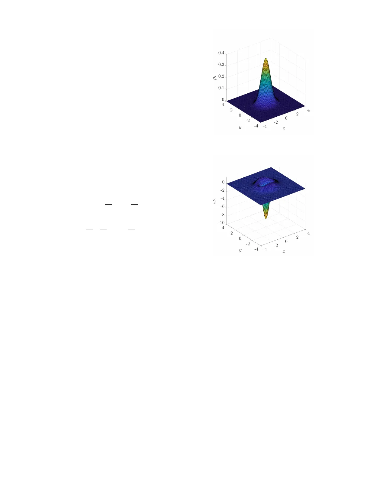
Optimal Contr ol f or Steady Cir culation of a Diffusion Pr ocess via Spectral Decomposition of F okk er –Planck Equation Norihisa Namura and Hiroya Nakao Abstract — W e present a formulation of an optimal control problem f or a two-dimensional diffusion process go verned by a Fokk er –Planck equation to achieve a nonequilibrium steady state with a desired cir culation while accelerating conv ergence toward the stationary distribution. T o achieve the control objec- tive, we introduce costs f or both the probability density function and flux rotation to the objectiv e functional. W e formulate the optimal control problem through dimensionality reduction of the Fokker –Planck equation via eigenfunction expansion, which requir es a low-computational cost. W e demonstrate that the proposed optimal control achieves the desired circulation while accelerating conv ergence to the stationary distribution through numerical simulations. I . I N T RO D U C T I O N In the real world, a wide range of systems are affected by stochastic noise. Examples include nerve signal transmission by stochastically opening and closing ion channels [1], electronic circuits subjected to thermal fluctuations [2], semi- classically approximated quantum dissipativ e systems [3], and robots subjected to their sensor and actuator noise [4]. Random fluctuations often appear as Bro wnian motion, where particles under go irregular motion due to collisions with surrounding molecules. The state dynamics of a Bro w- nian particle is mathematically described by the It ˆ o stochastic differential equation and the time ev olution of the probability density function (PDF) of the particles can be described by the corresponding F okker –Planck equation (FPE) [5]. Formulating control that acts on the FPE is useful [6] and numerous studies hav e formulated optimal control problems for FPEs [7], [8], [9], [10]. Optimal control is a general and valuable control approach that has found wide applications, including in the control of oscillatory systems [11], [12]; howe ver , it is difficult to solve optimal control problems in infinite-dimensional systems. Since FPE is linear , it can be analyzed using the eigen values and eigenfunctions [5]. By using a spectral approach to the FPE, we can approximately formulate optimal control problems, such as for fast con vergence to the stationary distribution [13], [14], [15]. In thermodynamically equilibrium systems, detailed bal- ance ensures that no flux exists in the stationary state, N. Namura is with the Department of Systems and Control Engineering, Institute of Science T okyo, T okyo, Japan (namura.n.aa@m.titech.ac.jp) H. Nakao is with the Department of Systems and Control Engineering and Research Center for Autonomous Systems Materialogy , Institute of Science T okyo, T okyo, Japan (nakao@sc.e.titech.ac.jp) N. Namura acknowledges the support from JSPS KAKENHI (No. 25KJ1270). H. Nakao acknowledges the support from JSPS KAKENHI (Nos. 25H01468, 25K03081, and 22H00516). such as the circulation of the particles. Introducing circula- tions, howe ver , allo ws us to enhance efficiency of particle mixing [16] or capturing particles in target regions [16], [17]. Hence, generating circulations by dri ving the system in a nonequilibrium state can improve the performance and functional capabilities of the system, rather than merely achieving equilibrium state. In this study , we formulate an optimal control problem for a two-dimensional diffusion process described by the FPE to achie ve two control objecti ves: (i) accelerating the con vergence of the PDF tow ard a stationary state, and (ii) generating a desired circulation when the PDF is in the stationary state. In addition to the cost functional for accelerating conv ergence to the stationary distrib ution intro- duced in [15], a term that accounts for the difference from the desired flux rotation (scalar vorticity [18]) is added in the objective functional. In the formulation, we utilize the eigenfunction expansion of the PDF with a finite number of eigenfunctions for dimensionality reduction, which is ex- pected to significantly reduce the computational cost during optimization. Through numerical simulations, we demon- strate that the formulated optimal control problem allows the PDF to con ver ge quickly to its stationary state, while simultaneously generating the desired circulation. This study is organized as follows. W e first introduce a diffusion process and the corresponding FPE in Sec. II. In Sec. III, we propose an optimal control scheme to accelerate con vergence to the stationary distribution while generating a desired circulation based on the spectral dimensionality reduction of the FPE. In Sec. IV, we demonstrate that the control objecti ve is achiev ed by the optimal control compared to the uncontrolled case through numerical simulations. W e conclude this study in Sec. V. I I . F O K K E R – P L A N C K E Q UA T I O N W e consider a two-dimensional diffusion process { X t } t ≥ 0 on a simply connected compact set Ω ⊂ R 2 with a smooth boundary Γ , where each state variable is independently subjected to white Gaussian noise. This diffusion process can be described by the follo wing It ˆ o stochastic differential equation (SDE): d X t = −∇ V ( X t ) dt + √ 2 D d W t , (1) where t ∈ R + = [0 , ∞ ) represents the time, V : Ω → R is a smooth potential function, D > 0 is a diffusion con- stant, ∇ = [ ∂ x ∂ y ] ⊤ represents the gradient for the spatial variable x = [ x y ] ⊤ ∈ Ω , ∂ x = ∂ /∂ x represents the partial deriv ativ e with respect to x , “ ⊤ ” represents the transposition of a vector or matrix, and { W t } t ≥ 0 represents a standard two-dimensional Brownian motion. The time ev olution of the probability density function (PDF) ρ : Ω × R + → R + of X t is described by the Fokk er–Planck equation (FPE): ∂ t ρ ( x , t ) = L ∗ ρ = ∇ · ( ρ ( x , t ) ∇ V ( x )) + D ∆ ρ ( x , t ) (2) by using a linear operator L ∗ = ∇ · ∇ V + D ∆ , where a · b = a 1 b 1 + a 2 b 2 is the scalar product of two-dimensional vectors a , b and ∆ = ∇ · ∇ is the Laplacian operator . W e then define a probability flux J : Ω × R + → R 2 to satisfy L ∗ ρ ( x , t ) = −∇ · J ( x , t ) . (3) For the flux J , we consider the reflecting boundary condition on the boundary Γ at any t , i.e., J ( x , t ) · n = 0 on Γ × R + , (4) where n represents the normal vector perpendicular to Γ . In equilibrium systems, the stationary flux J s satisfies the detailed balance condition J s ( x ) = 0 for any x ∈ Ω when the PDF is stationary , ρ ( x , t ) = ρ s ( x ) . In this case, the linear operator L ∗ is self-adjoint with respect to the weighted square-integrable function space L 2  Ω; ρ − 1 s  [19], [14], [15]. The stationary distribution is given by ρ s ( x ) = 1 Z exp  − V ( x ) D  , (5) where Z = R Ω exp  − V ( x ) D  d x is a normalization constant and d x = dxdy is the integration measure. W e can consider the set of the eigenv alues and eigenfunc- tions { ( λ m , v m ) } , ( m = 0 , 1 , 2 , . . . ) of L ∗ that satisfies L ∗ v m = λ m v m , (6) where { λ m } are sorted as Re λ 0 ≥ Re λ 1 ≥ · · · . The eigen- functions { v m } can be orthonormalized on L 2  Ω; ρ − 1 s  as follows: ⟨ v m , v k ⟩ L 2 ( Ω; ρ − 1 s ) = δ mk , (7) where ⟨ p, q ⟩ L 2 ( Ω; ρ − 1 s ) = R p ( x ) q ( x ) ρ − 1 s ( x ) d x is the inner product of two functions p, q on L 2  Ω; ρ − 1 s  , the ov erline represents the complex conjugate, and δ mk is the Kronecker delta. Since the stationary distribution satisfies L ∗ ρ s = 0 , ρ s is the eigenfunction that corresponds to the zero eigen value, i.e., λ 0 = 0 and v 0 = ρ s . I I I . F O R M U L A T I O N O F O P T I M A L C O N T RO L A. Contr ol Objective Our control objective is to accelerate the conv ergence speed of the PDF toward the stationary state and gener- ate a desired circulation from the initial time t 0 ≥ 0 until the final time t f > t 0 . For this purpose, we consider a diffusion process with control { X t } t ≥ 0 described by the following It ˆ o SDE (8) whose drift term recei ves the control inputs u 1 , 2 ∈ L 2 ([ t 0 , t f ]) with control shape functions [14] α and ϕ : d X t =  − u 1 ( t ) ∇ α ( X t ) − u 2 ( t ) 1 ρ s ( X t ) ∇ ⊥ ϕ ( X t )  dt − ∇ V ( X t ) dt + √ 2 D dW t , (8) where ∇ ⊥ = [ ∂ y − ∂ x ] is a partial deriv ativ e operator that is perpendicular to ∇ . The term with u 1 mainly serves to accelerate the con vergence, whereas the term with u 2 generates a circulation in the steady state. Note that the control inputs u 1 , 2 depend only on time and regulate the intensity of the smooth control shape functions α : Ω → R and ϕ : Ω → R , respectively . W e assume that the controlled SDE (8) admits a unique solution. The FPE corresponding to the SDE (8) is gi ven by ∂ t ρ = ∇ ·  ρ  ∇ V + u 1 ∇ α + u 2 1 ρ s ∇ ⊥ ϕ  + D ∆ ρ (9) and the probability flux ˜ J under the control is described by ˜ J = − ρ  ∇ V + u 1 ∇ α + u 2 1 ρ s ∇ ⊥ ϕ  − D ∇ ρ. (10) Here, we assume that the control shape functions satisfy the following boundary conditions: ∇ α · n = 0 on Γ , (11) ∇ ⊥ ϕ · n = 0 on Γ , (12) in order that ˜ J satisfies the reflecting boundary condition ev en under the control, i.e., ˜ J ( x , t ) · n = 0 on Γ × R + . (13) W e assume the well-posedness of the controlled FPE (9) with the boundary condition (13). The control objectiv e includes fast con vergence to the sta- tionary distribution ρ s of the uncontrolled system. Here, we consider that the system to hav e conv erged to the stationary state when ρ is sufficiently close to ρ s within a finite time. The stationary flux ˜ J s in the stationary state with ρ = ρ s should satisfy the follo wing condition for all x ∈ Ω , i.e., ∇ · ˜ J s ( x ) = 0 . (14) For this condition to hold, it is sufficient that the following two equations are satisfied: u 1 ∇ · ( ρ s ∇ α ) = 0 , (15) u 2 ∇ ·  ∇ ⊥ ϕ  = 0 . (16) In general, ∇ · ( ρ s ∇ α ) does not v anish but it is sufficient that the condition (15) is satisfied when u 1 = 0 , because u 1 becomes practically zero after the sufficient con vergence of ρ to ρ s . Meanwhile, the condition (16) is always satisfied because ∇ ·  ∇ ⊥ ϕ  = 0 holds for any smooth function ϕ : Therefore, when u 1 = 0 , ρ s is still a stationary distribution of the FPE (9) e ven for u 2  = 0 . T o generate a desired circulation, we control the system so that the flux rotation ω ( x , t ) = ∇ × ˜ J ( x , t ) reaches a de- sired flux rotation ω d ( x ) in the steady state with ρ = ρ s . The term ∇ × ˜ J ( x , t ) yields a scalar quantity in two dimensions and satisfies ∇ × ˜ J ( x , t ) = −∇ ⊥ · ˜ J ( x , t ) . Here, the flux rotation satisfies R Ω ω ( x , t ) d x = 0 at any t and we further assume that ω ( · , t ) ∈ L 2  Ω; ρ − 1 s  . Since we can assume u 1 = 0 when ρ = ρ s , the stationary flux for a constant u 2 satisfies ˜ J s = − u 2 ∇ ⊥ ϕ and the stationary flux rotation satisfies ω s = ∇ × ˜ J s = u 2 ∇ ⊥ · ∇ ⊥ ϕ = u 2 ∆ ϕ , whose shape depends only on ϕ . Thus, we can achiev e any smooth desired flux rotation ω d = ∆ ϕ by appropriately designing the shape function ϕ . In this case, the control objectiv e can be set as u 2 = 1 . In this study , we assume the controllability of the system to the nonequilibrium steady state characterized by the stationary distrib ution ρ s and the desired flux rotation ω d . W e note that the detailed balance condition does not hold in the steady state under the control, but we can discuss the controlled FPE (9) using the f act that the detailed balance condition J s = 0 holds in the original uncontrolled system. B. Spectral Dimensionality Reduction W e consider the eigenfunction expansion of the PDF ρ using the eigenfunctions { v m } of the linear operator L ∗ as ρ ( x , t ) = ∞ X m =0 c m ( t ) v m ( x ) , (17) where each coef ficient c m can be obtained by c m ( t ) = ⟨ ρ ( · , t ) , v m ⟩ L 2 ( Ω; ρ − 1 s ) . (18) By defining ζ 1 , 2 as ζ 1 ( x , t ) = ∇ · ( ρ ( x , t ) ∇ α ( x )) , (19) ζ 2 ( x , t ) = ∇ ·  ρ ( x , t ) 1 ρ s ( x ) ∇ ⊥ ϕ ( x )  , (20) the controlled FPE (9) can be re written as ∂ t ρ = L ∗ ρ + u 1 ζ 1 + u 2 ζ 2 : = F { ρ, u 1 , u 2 } , (21) where F describes the dynamics of the controlled FPE. The dynamics of each coefficient c m can then be described by the follo wing ordinary differential equation (ODE): ˙ c m = λ m c m + u 1 ⟨ ζ 1 ( · , t ) , v m ⟩ L 2 ( Ω; ρ − 1 s ) + u 2 ⟨ ζ 2 ( · , t ) , v m ⟩ L 2 ( Ω; ρ − 1 s ) = λ m c m + u 1 ∞ X k =0 c k ⟨∇ · ( v k ∇ α ) , v m ⟩ L 2 ( Ω; ρ − 1 s ) + u 2 ∞ X k =0 c k  ∇ ·  v k ρ s ∇ ⊥ ϕ  , v m  L 2 ( Ω; ρ − 1 s ) , (22) where ˙ c m represents the time deri vati ve of c m . Hereafter , we consider a finite set of M eigen val- ues { λ m } M − 1 m =0 and corresponding eigenfunctions { v m } M − 1 m =0 for the purpose of dimensionality reduction. W e define a coefficient vector and an eigen value matrix by c =  c 0 c 1 · · · c M − 1  ⊤ ∈ R M , (23) Λ = diag( λ 0 , λ 1 , . . . , λ M − 1 ) ∈ R M × M , (24) respectiv ely , and introduce matrices B 1 , 2 ∈ R M × M , where the ( m, k ) -components B ( mk ) 1 , 2 of the matrices are gi ven by B ( mk ) 1 = ⟨∇ · ( v k ∇ α ) , v m ⟩ L 2 ( Ω; ρ − 1 s ) , (25) B ( mk ) 2 =  ∇ ·  v k ρ s ∇ ⊥ ϕ  , v m  L 2 ( Ω; ρ − 1 s ) , (26) respectiv ely . Finally , the controlled FPE (9) can be approxi- mated by the follo wing ODE: ˙ c = Λ c + u 1 B 1 c + u 2 B 2 c : = f ( c , u 1 , u 2 ) . (27) The ODE (27) driv en by the vector field f is a bilinear system with the state c and control inputs u 1 , 2 . C. Optimization T o achiev e the control objectiv e, we introduce a stage cost functional L 1 for the PDF , which is described using a weight Q 1 > 0 as follo ws: L 1 [ ρ ] = Q 1 2 | ρ ( · , t ) − ρ s | 2 L 2 ( Ω; ρ − 1 s ) , (28) where |·| L 2 ( Ω; ρ − 1 s ) represents the L 2  Ω; ρ − 1 s  norm. In addition, we introduce a stage cost functional L 2 for the flux rotation, which is described using a weight Q 2 > 0 as follows: L 2 [ ω ] = Q 2 2 | ω ( · , t ) − ω d | 2 L 2 ( Ω; ρ − 1 s ) = Q 2 2    ∇ × ˜ J ( · , t ) − ω d    2 L 2 ( Ω; ρ − 1 s ) . (29) W e also introduce a terminal cost functional φ for the PDF and flux rotation using a similar formulation as φ [ ρ ( · , t f ) , ω ( · , t f )] = Q f 2 | ρ ( · , t f ) − ρ s | 2 L 2 ( Ω; ρ − 1 s ) + R f 2 | ω ( · , t f ) − ω d | 2 L 2 ( Ω; ρ − 1 s ) . (30) Finally , we introduce a stage cost function L 3 for the inputs u 1 , 2 using weights R 1 , 2 > 0 as follo ws: L 3 ( u 1 ( t ) , u 2 ( t )) = 1 2 R 1 u 1 ( t ) 2 + 1 2 R 2 u 2 ( t ) 2 . (31) Hence, the objecti ve functional J is represented as J [ u 1 , u 2 ] = φ [ ρ ( · , t f ) , ω ( · , t f )] + Z t f t 0 L 1 [ ρ ] + L 2 [ ω ] + L 3 ( u 1 , u 2 ) dt. (32) The optimal control problem is formulated as min u 1 ,u 2 J [ u 1 , u 2 ] s . t . ∂ t ρ = F { ρ, u 1 , u 2 } , ρ ( t 0 ) = ρ 0 , (33) where ρ 0 is the initial PDF at t 0 . The proposed optimal control problem satisfies the standard conditions ensuring the existence of an optimal control, namely coercivity and weak lower semicontinuity of the cost functional together with continuity of the control-to-state mapping [20], [15]. Next, we reformulate the objectiv e functional by using the eigenfunction expansion (17) of the PDF ρ . The stage cost for the PDF can be approximated by a function ˜ L 1 of the coefficient vector c as L 1 [ ρ ] ≈ ˜ L 1 ( c ) = Q 1 2 * M − 1 X m =0  c m − c ( m ) s  v m , M − 1 X k =0  c k − c ( k ) s  v k + L 2 ( Ω; ρ − 1 s ) = Q 1 2 ∥ c − c s ∥ 2 , (34) where the m -th component of the v ector c s ∈ R M is obtained as c ( m ) s = ⟨ ρ s , v m ⟩ L 2 ( Ω; ρ − 1 s ) and ∥·∥ represents the Euclid norm of a M -dimensional vector . The stage cost for the flux rotation can also be approximated by a function ˜ L 2 of c and u 1 , 2 by calculating the flux ˜ J using the eigenfunction expansion (17), which can be written as L 2 [ ω ] ≈ ˜ L 2 ( c , u 1 , u 2 ) = Q 2 2 ∥ ( A 1 + u 1 ( t ) A 2 + u 2 ( t ) A 3 ) c − d ∥ 2 . (35) Here, each component of the matrices A 1 , 2 , 3 ∈ R M × M and the vector d ∈ R M is represented as A ( mk ) 1 =  ∇ ⊥ v m · ∇ V , v k  L 2 ( Ω; ρ − 1 s ) , (36) A ( mk ) 2 =  ∇ ⊥ v m · ∇ α, v k  L 2 ( Ω; ρ − 1 s ) , (37) A ( mk ) 3 =  ∇ ⊥ v m ρ s · ∇ ⊥ ϕ + v m ρ s ∆ ϕ, v k  L 2 ( Ω; ρ − 1 s ) , (38) d ( k ) = ⟨ ω d , v k ⟩ L 2 ( Ω; ρ − 1 s ) , (39) respectiv ely , because the flux ˜ J can be approximated as ˜ J ≈ − M − 1 X m =0 c m v m  ∇ V + u 1 ∇ α + u 2 1 ρ s ∇ ⊥ ϕ  − D M − 1 X m =0 c m ∇ v m . (40) Since u 2 = 1 is the control objectiv e for the flux rotation in the stationary state, the terminal cost can be approximated as φ [ ρ ( · , t f ) , ω ( · , t f )] ≈ ˜ φ ( c ( t f ) , u 2 ( t f )) = Q f 2 ∥ c ( t f ) − c s ∥ 2 + R f 2 ( u 2 ( t f ) − 1) 2 . (41) Hence, the objecti ve functional can be approximated as J [ u 1 , u 2 ] ≈ ˜ J [ u 1 , u 2 ] = ˜ φ ( c ( t f ) , u 2 ( t f )) + Z t f t 0 ˜ L 1 ( c ) + ˜ L 2 ( c , u 1 , u 2 ) + L 3 ( u 1 , u 2 ) dt. (42) The objectiv e functional includes the product of c and u 1 , 2 but is still coercive. Thus, the lo w-dimensional optimal control problem can be formulated with a Lagrange multiplier vector µ ( t ) ∈ R M as min u 1 ,u 2 ˜ J [ u 1 , u 2 ] + Z t f t 0 µ ( t ) ⊤ ( f ( c , u 1 , u 2 ) − ˙ c ( t )) dt s . t . c ( t 0 ) = c 0 , (43) giv en that the initial condition at t 0 for the state c satisfies c ( t 0 ) = c 0 , (44) where c 0 is the initial state corresponding to ρ 0 and its m -th component is obtained as ( c 0 ) ( m ) = ⟨ ρ 0 , v m ⟩ L 2 ( Ω; ρ − 1 s ) . Theor em 1: In the M → ∞ limit, any optimal solution of the approximated problem (43) con ver ges to an optimal solution of the original problem (33). Pr oof: Since the eigenfunction expansion of ρ up to m = M − 1 con ver ges to ρ as M → ∞ in L 2  Ω; ρ − 1 s  space [19], the cost function ˜ L 1 con verges to the cost func- tional L 1 . Since the flux ˜ J can be expanded as Eq. (40) and ω ( x , t ) = −∇ ⊥ · ˜ J ( x , t ) , the cost function ˜ L 2 con verges to the cost functional L 2 . Similarly , the cost function ˜ φ con verges to the cost functional φ . Therefore, the value of ˜ J con verges to that of J . Since ˜ J is coerciv e independently of M , any optimal solution of (43) remains bounded for all M and con verges to an optimal solution of (33). Defining the Hamiltonian H ( c , u 1 , u 2 , µ ) by H ( c , u 1 , u 2 , µ ) = ˜ L 1 ( c ) + ˜ L 2 ( c , u 1 , u 2 ) + L 3 ( u 1 , u 2 ) + µ ( t ) ⊤ f ( c , u 1 , u 2 ) , (45) the dynamics of µ can be described by the following ODE: ˙ µ = −∇ c H ( c , u 1 , u 2 , µ ) (46) and µ satisfies the terminal condition: µ ( t f ) = ∇ c H ( c ( t f ) , u 2 ( t f )) , (47) where ∇ c is the gradient with respect to c . Since it is difficult to obtain the optimal solution analyt- ically , we numerically obtained it using the MA TLAB opti- mization solver fminunc . At each step of the optimization, the state equation (27) is first numerically integrated from t = t 0 to t = t f using the Euler method with the initial con- dition (44), and then the ODE for µ gi ven by (46) is solved from t = t f to t = t 0 with the terminal condition (47), to ev aluate the v alue of the objective functional ˜ J . Finally , we obtained a local optimal solution that satisfies the stationarity condition of the Hamiltonian with respect to the inputs, i.e., ∂ H /∂ u 1 , 2 = 0 for all t ∈ [ t 0 , t f ] . Although this optimization problem is not con ve x, the formulated optimization problem requires low computational cost owing to the dimensionality reduction of the original problem. I V . R E S U L T S W e demonstrate through numerical simulations that the FPE (9) under the optimal control obtained by the pro- posed formulation suf ficiently achieves the control ob- jectiv e. As an e xample, we consider a controlled dif fu- sion process (8) with the potential V ( x ) = 2 x 2 + 3 y 2 and diffusion constant D = 2 . W ithout control, the FPE (2) has a stationary PDF ρ s as sho wn in Fig. 1 on a do- main Ω = [ − L, L ] × [ − L, L ] with a length L = 4 . For nu- merical simulations, the x and y components are discretized with interv als ∆ x = 0 . 08 and ∆ y = 0 . 08 , respecti vely . The control objective is to accelerate con ver gence to ward the stationary distribution ρ s and generate a desired flux rotation ω d as sho wn in Fig. 2 from the initial time t 0 = 0 until the final time t f = 1 . Here, the control shape functions are set as α ( x ) = cos  π x 2 L  cos  π y 2 L  (48) and ϕ ( x ) = ρ s L 2 4  x 2 L 2 − 1   y 2 L 2 − 1  , (49) which satisfy the boundary conditions. The initial distri- bution is taken as a mixture of two truncated and nor- malized Gaussian PDFs with equal weights; one has a mean [1 0] ⊤ and covariance matrix diag(0 . 5 , 0 . 5) and the other has a mean [ − 1 0] ⊤ and the same covari- ance. W e approximate the PDF driv en by the controlled FPE (9) using M = 21 eigenfunctions corresponding to the M = 21 largest real eigenv alues. W e performed optimization with the weights Q f = 10 2 , R f = 1 , Q 1 = 10 4 , Q 2 = 10 , R 1 = 1 , and R 2 = 1 from an initial guess u 1 ( t ) = 0 and u 2 ( t ) = 1 . In the optimization, we numerically integrate the ODEs (27) and (46) by the Euler method with a time step ∆ t = 5 × 10 − 3 . W e show the optimal control inputs in Figs. 3(a) and (b). The input u 1 increases from a large negati ve value to 0 in the initial stage, indicating that it is optimal to apply a large input in the early state to accelerate the con vergence of ρ to wards ρ s . Meanwhile, the input u 2 increases from 0 and con verges to 1 after the initial stage, indicating that it is optimal to generate the desired circulation when the PDF sufficiently con vergences to the target ρ s . W e numerically integrated the FPE (9) using the obtained optimal control inputs by the implicit method with the time step ∆ t . W e compare the optimal control and uncontrolled cases by calculating the L 2  Ω; ρ − 1 s  norm e ρ = | ρ ( · , t ) − ρ s | L 2 ( Ω; ρ − 1 s ) for the PDF and L 2  Ω; ρ − 1 s  norm e ω = | ω ( · , t ) − ω d | L 2 ( Ω; ρ − 1 s ) for the flux rotation. W e can find that the control objecti ve Fig. 1. Stationary distribution ρ s of the uncontrolled FPE. Fig. 2. Desired flux rotation ω d . is successfully achiev ed by using the optimal control inputs. W e note that the initial values of the e ω are different between the optimal control and uncontrolled cases because the flux rotation is af fected by the control inputs. Furthermore, we numerically integrated the time ev olution of 10 5 independent particles governed by the controlled SDE (8) using the Euler–Maruyama method with the time step ∆ t . W e then computed the flux at the final time, which can be obtained from the particle states by calculating the drift term by the sample mean of the displacement at each grid domain and approximating the histogram by a truncated Gaussian mixture model. W e show the flux under optimal control at the final time in Fig. 5, where the flux successfully exhibits clockwise rotation around the origin, corresponding to ω d being negati ve near the origin. V . C O N C L U S I O N S In this study , we formulated an optimal control problem for a diffusion process described by a two-dimensional It ˆ o SDE to achiev e a desired circulation while accelerating con vergence to the stationary distribution of the original circulation-free Fokker –Planck equation. By the formulation 0 0.5 1 t -60 -40 -20 0 u 1 0 0.5 1 t 0 0.5 1 u 2 (a) (b) Fig. 3. Optimal control inputs. (a) Optimal control input u 1 . The horizontal line represents u 1 ( t ) = 0 . (b) Optimal control input u 2 . The horizontal line represents u 2 ( t ) = 1 . 0 0. 5 1 t -0.5 0 0.5 1 1.5 2 e ; uncontrolled optimal control 0 0. 5 1 t -10 0 10 20 30 40 50 e ! uncontrolled optimal control (a) (b) Fig. 4. Comparison of the L 2  Ω; ρ − 1 s  norm between the uncontrolled case and optimal control case. (a) L 2  Ω; ρ − 1 s  norm between the station- ary and current distribution. (b) L 2  Ω; ρ − 1 s  norm between the desired and current flux rotation. -4 -2 0 2 4 x -4 -2 0 2 4 y Optimal c ontrol Fig. 5. The behavior of the flux obtained from the particles under the optimal control at the final time on the xy plane. The length of the arrows represents the flux speed. of the optimal control problem based on dimensionality reduction via the eigenfunction expansion of the probability density function, we demonstrated that the control objecti ve can be achiev ed through numerical simulations. Although the desired flux rotation can also be achie ved while ensuring con- ver gence to the stationary distribution by the trivial choice of the control inputs, u 1 ( t ) = 0 and u 2 ( t ) = 1 , it is worthwhile to solve the optimal control problem because a different and more ef ficient optimal solution (Fig. 3) was obtained when the tri vial choice was used as the initial guess in the numerical example. A future work would be to formulate optimal control problems for the similar control objecti ve in three or higher-dimensional cases and inv estigate a nonlinear FPE under particle interactions. R E F E R E N C E S [1] G. B. Ermentrout and D. H. T erman, Mathematical F oundations of Neur oscience . New Y ork: Springer, 2010. [2] C. Gardiner, Stochastic Methods . Berlin: Springer , 2009, vol. 4. [3] Y . Kato, N. Y amamoto, and H. Nakao, “Semiclassical phase reduction theory for quantum synchronization, ” Phys. Rev . Res. , vol. 1, p. 033012, Oct 2019. [4] K. Elamvazhuthi and S. Berman, “Mean-field models in swarm robotics: a surv ey , ” Bioinspiration & Biomimetics , vol. 15, no. 1, p. 015001, nov 2019. [5] H. Risken, F okker –Planck Equation . Springer Berlin Heidelberg, 1996, pp. 63–95. [6] M. Annunziato and A. Borz ` ı, “ A Fokker –Planck control framework for stochastic systems, ” EMS Surve ys in Mathematical Sciences , v ol. 5, no. 1, pp. 65–98, 2018. [7] M. Annunziato and A. Borz ` ı, “Optimal control of probability den- sity functions of stochastic processes, ” Mathematical Modelling and Analysis , vol. 15, no. 4, pp. 393–407, 2010. [8] M. Annunziato and A. Borz ` ı, “ A Fokker–Planck control framework for multidimensional stochastic processes, ” Journal of Computational and Applied Mathematics , vol. 237, no. 1, pp. 487–507, 2013. [9] A. Fleig and R. Guglielmi, “Optimal control of the Fokker –Planck equation with space-dependent controls, ” Journal of Optimization Theory and Applications , vol. 174, no. 2, pp. 408–427, 2017. [10] T . Breiten and K. K. Kunisch, “Improving the conver gence rates for the kinetic Fokker–Planck equation by optimal control, ” SIAM Journal on Contr ol and Optimization , vol. 61, no. 3, pp. 1557–1581, 2023. [11] J. Moehlis, E. Shea-Brown, and H. Rabitz, “Optimal inputs for phase models of spiking neurons, ” Journal of Computational and Nonlinear Dynamics , vol. 1, no. 4, pp. 358–367, 06 2006. [12] N. Namura and H. Nakao, “Optimal phase control of limit-cycle oscillators with strong inputs through phase-amplitude reduction, ” in 2024 IEEE 63r d Confer ence on Decision and Contr ol (CDC) , 2024, pp. 4003–4009. [13] T . Breiten, K. Kunisch, and L. Pfeiffer , “ A reduction method for Riccati-based control of the Fokker –Planck equation, ” IF AC- P apersOnLine , vol. 50, no. 1, pp. 1631–1636, 2017. [14] T . Breiten, K. Kunisch, and L. Pfeiffer , “Control strategies for the Fokker –Planck equation, ” ESAIM: COCV , vol. 24, no. 2, pp. 741– 763, 2018. [15] D. Kalise, L. M. Moschen, G. A. Pavliotis, and U. V aes, “ A spectral approach to optimal control of the Fokker –Planck equation, ” IEEE Contr ol Systems Letters , vol. 9, pp. 504–509, 2025. [16] Y . Lu, W . T an, S. Mu, and G. Zhu, “V ortex-enhanced microfluidic chip for efficient mixing and particle capturing combining acoustics with inertia, ” Analytical Chemistry , vol. 96, no. 9, pp. 3859–3869, 2024. [17] W . Zhang et al. , “V orte x-induced particle capture in a micro cross- shaped channel, ” Separation and Purification T echnology , vol. 336, p. 126245, 2024. [18] F . Flandoli, F . Grotto, and D. Luo, “Fokker –Planck equation for dissipativ e 2D Euler equations with c ylindrical noise, ” Theory of Pr obability and Mathematical Statistics , vol. 102, pp. 117–143, 2020. [19] G. A. Pavliotis, “Stochastic processes and applications, ” 2014. [20] J. L. Lions, Optimal Control of Systems Governed by P artial Differ- ential Equations . Springer Berlin, Heidelberg, 1971.