Consistency of the $k$-Nearest Neighbor Regressor under Complex Survey Designs

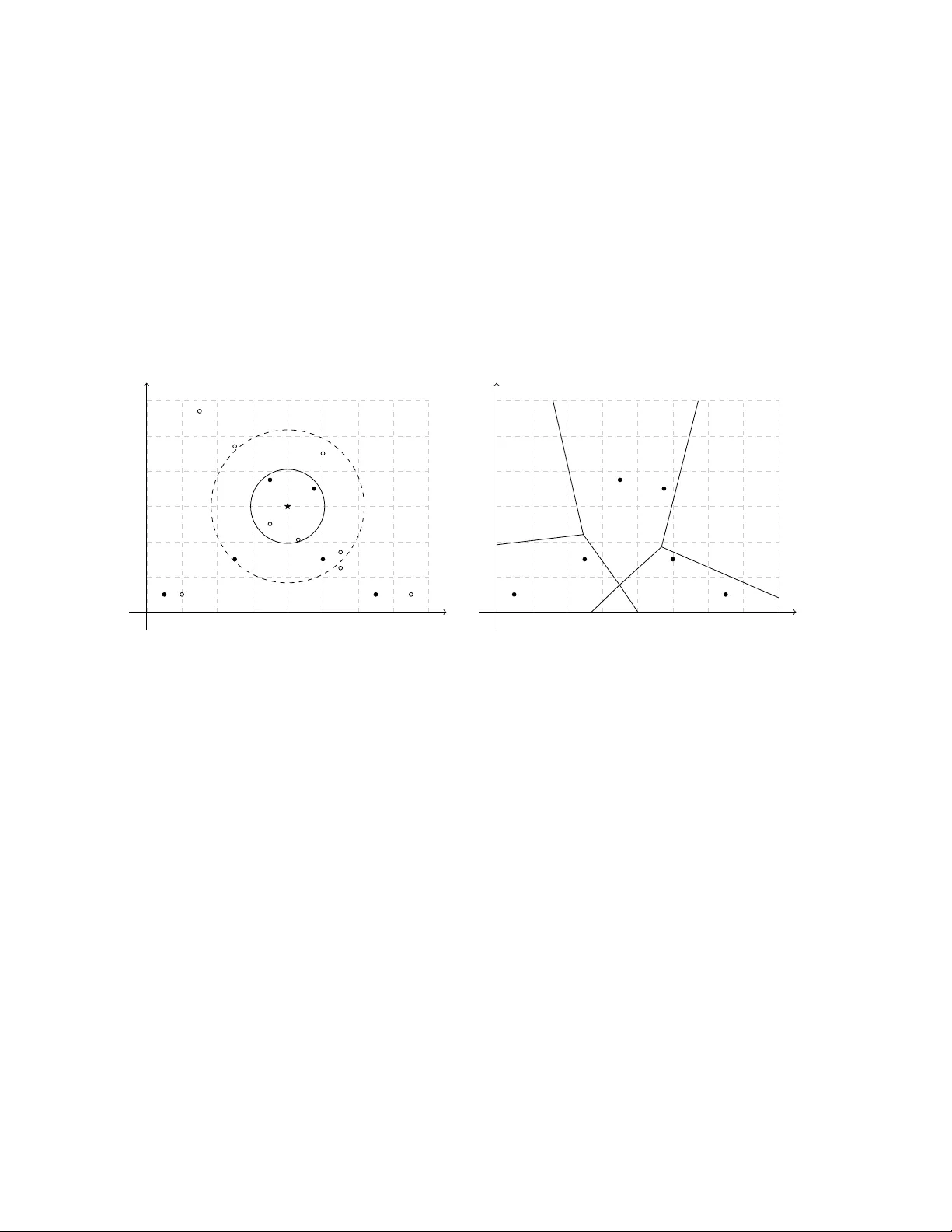
Consistency of the k -Nearest Neigh b or Regressor under Complex Surv ey Designs Caren Hasler Marc h 19, 2026 Abstract W e study the consistency of the k -nearest neighbor regressor under complex survey designs. While consistency results for this algorithm are w ell established for indep en- den t and identically distributed data, corresponding results for complex survey data are lacking. W e show that the k -nearest neigh b or regressor is consistent under regu- larit y conditions on the sampling design and the distribution of the data. W e derive lo wer b ounds for the rate of conv ergence and sho w that these b ounds exhibit the curse of dimensionality , as in the indep endent and identically distributed setting. Empirical studies based on sim ulated and real data illustrate our theoretical findings. Keyw ords : Complex survey data, Survey sampling, Design-based inference, Sup erp op- ulation mo del, Conv ergence, Nonparametric regression. 1 In tro duction The k -Nearest Neighbors ( k -NN) algorithm is a non-parametric sup ervised learning metho d for classification and regression. As a classifier, k -NN assigns a unit to the most common 1 class among its k nearest neigh b ors. As a regressor, it predicts a unit’s v alue by av eraging the observ ed v alues of its k nearest neighbors. T o the b est of our knowledge, the first formalization of k -NN is found in the seminal work of Fix and Ho dges ( 1951 ). Since then, in terest in k -NN has grown rapidly in a wide range of fields, with survey sampling b eing no exception. Statistical consistency is a crucial asymptotic prop ert y . An estimator is consistent if it b ecomes more tigh tly concen trated around the parameter it in tends to estimate as the sample size increases. The literature dev oted to the consistency and other asymptotic prop erties of the k -NN classifier and regressor is v ast. Indeed, since the seminal work of Stone ( 1977 ) on the consistency of nonparametric regression estimators, including k -NN, the sub ject has b een the fo cus of n umerous studies. T o cite only a few of those, Devroy e et al. ( 1996 ); Hall et al. ( 2008 ); Samw orth ( 2012 ); Gadat et al. ( 2016 ); D¨ oring et al. ( 2018 ); Gy¨ orfi and W eiss ( 2021 ) presen t some asymptotic prop erties of the k -NN classifier and Mack ( 1981 ); Devroy e et al. ( 1994 ); Biau et al. ( 2010 , 2012 ) study those of the k -NN regressor. The b o ok of Biau and Devroy e ( 2015 ) is dev oted to k -NN and discusses its asymptotic prop erties in depth. All of the asymptotic results presented in the aforementioned studies are derived in a pure mo del-based framew ork, where the data are indep enden t and iden tically distributed (i.i.d.). In this framework, a mo del for the data is assumed and the sample is view ed as a collection of dra ws of i.i.d. random v ariables. The p opulation is treated as infinite, and the randomness comes from the data-generating pro cess. In a design-based framework, ho w ever, the p opulation is treated as finite and fixed. The sample data, or surv ey data, are selected at random from this p opulation with a complex selection scheme, often without replacement and with unequal probabilities. The randomness then arises from the sampling pro cess. Th us, the i.i.d. assumption do es not hold for surv ey data. Given these differences, the asymptotic results ab out k -NN developed in a pure mo del-based framew ork are generally not directly v alid in a design-based framework. T o b e v alid for surv ey data, asymptotic results ab out k -NN need to b e tailored to the design-based framew ork. 2 Despite the considerable interest in k -NN among surv ey researc hers and practitioners, asymptotic results remain limited and, to the best of our kno wledge, are a v ailable only in t w o con texts: imputation for nonresp onse and spatial mapping in en vironmen tal studies. In the con text of imputation for nonresp onse, missing v alues of nonresp onden ts are imputed using k -NN applied to the respondents. Five published papers examine asymptotic prop erties of k - NN imputation in surv eys. Chen and Shao ( 2000 ) presen t asymptotic properties of the 1-NN imputation metho d for functions of p opulation means (or totals), p opulation distributions, and p opulation quan tiles. Chen and Shao ( 2001 ) prop ose t wo asymptotically unbiased and consisten t jac kknife v ariance estimators for 1-NN imputation. Shao and W ang ( 2008 ) deriv e asymptotic prop erties of the p oin t estimator, v ariance estimator, and confidence interv al for p opulation means and quantiles estimated via 1-NN imputation. These three papers rely on the somewhat unrealistic assumption of a single cov ariate. Tw o other pap ers extend these results to the case of multiple cov ariates. In order to b ypass the challenge of multiple cov ariates, Y ang and Kim ( 2019 ) assume that information con tained in the co v ariates can b e summarized b y a single scalar v ariable and apply 1-NN imputation to that v ariable. They study the asymptotic prop erties of the 1-NN imputation estimator for general p opulation parameters, including p opulation means, prop ortions, and quan tiles. Another solution to address m ultiple cov ariates is predictiv e mean matching. Predictiv e mean matching is implemen ted in t w o steps: 1) a mo del predicting the survey v ariable from the co v ariates is fitted using resp onden ts’ data, 2) 1-NN imputation is applied to the predicted surv ey v ariable obtained from the fitted mo del. Y ang and Kim ( 2020 ) study this alternative and establish some asymptotic prop erties of the predictive mean matc hing estimator. In the con text of en vironmental studies, k -NN is applied as an interpolator. Sp ecifically , it is used to map contin uous populations with finite p opulations of areas within a design- based framew ork, allowing estimation of the v alue of the surv ey v ariable at unsampled areas. F attorini et al. ( 2022 ) and F attorini et al. ( 2024 ) establish asymptotic properties of the k -NN 3 in terp olator in this context. The theoretical foundations of k -NN in the design-based framew ork are limited to the tw o aforemen tioned con texts. No theoretical foundations of the k -NN regressor or classifier ha ve b een deriv ed in the design-based framew ork, despite the growing num b er of applications. In this pap er, w e aim to bridge the gap b etw een theory and practice for k -NN in survey sampling. W e establish the asymptotic prop erties of the k -NN regressor under complex surv ey designs. W e adopt a sup erp opulation mo del approach. That is, we assume that the sample is obtained from a finite p opulation with a p ossibly-complex surv ey design, as in the design-based approac h. In addition, w e assume that the p opulation consists of realizations of i.i.d. random v ariables defined according to a model called the sup erp opulation mo del. The analysis is carried out according to b oth sources of randomness, namely the sampling design and the superp opulation mo del. In the case of the k -NN regressor, this choice seems natural. W e elab orate on this c hoice in Section 2 . In this pap er, we list conditions on the sampling design and on the distribution of the data under which the k -NN regressor is consistent. W e also provide lo wer b ounds for the rate of conv ergence of the k -NN regressor. Moreo v er, w e show that this estimator suffers from the curse of dimensionalit y , as in the traditional mo del-based approach. Finally , we present the results of empirical studies on sim ulated and real data, which illustrate and empirically supp ort our theoretical findings. This pap er is organized as follo ws. Section 2 con tains a description of the context and pieces of notation. Section 3 presents the k -NN regressor. The conditions required for consistency are listed and detailed in Section 4 . The main results on consistency and rate of con vergence are stated in Section 5 . The pro ofs are in the same section, with some tec hnical elemen ts left in the App endix . Section 6 presents the empirical studies carried out with sim ulated and true data. Concluding remarks are giv en in Section 7 . 4 2 Con text and Notation Let U v := { 1 , 2 , ...., N v } denote a finite p opulation of size N v . T o each elemen t i of U v , w e asso ciate a random v ector ( X i , Y i , Z i ) ∈ R p × R × R r . The co v ariates X i are v ariables used to predict the surv ey v ariable Y i . V ariables Z i are design v ariables used to construct the sampling design, see next paragraph. The finite p opulation data D U v := ( X i , Y i ) i ∈ U v are assumed to consist of i.i.d. realizations of a random vector ( X , Y ) generated from a sup erp opulation mo del ξ . F or simplicit y , we assume that the co v ariates and survey v ariable ha ve b ounded supp orts denoted by supp( X ) and supp( Y ), resp ectively . Let E ξ denote the exp ectation computed with resp ect to mo del ξ . A random sample S v of size n v is dra wn from U v using a sampling design p v ( · ). The sample data, or survey data, D S v := { ( X i , Y i ) } i ∈ S v are not i.i.d. The sample membership indicators are I v i = 1 i ∈ S v . F or generic units i and j in U v , the first- and second-order inclusion probabilities are π v i and π v ij , resp ectiv ely . W e build on the asymptotic framew ork of Isaki and F uller ( 1982 ) and consider that U v , v ∈ N is a sequence of embedded finite p opulations and the p opulation and sample sizes N v and n v gro w to infinity as v increases. The asso ciated sequence of samples S v ma y not b e em b edded. Hereafter, we omit subscript v to ease reading whenev er it is not confusing to do so. That is, we ma y write n for n v , N for N v , π i for π v i , and so on. W e will k eep in mind that these quan tities dep end on v . Let E p denote the exp ectation computed with resp ect to sampling design p conditionally on p opulation data D U v . In this pap er, w e consider the problem of estimating the regression function m ( x ) := E ξ E p [ Y | X = x ] for x ∈ supp( X ) from surv ey data D S v where E ξ E p is the exp ectation com- puted with resp ect to the distribution of the data and the sampling design. That is, w e consider the problem of estimating the mean of Y for given v alues of X . An example is the mean wage of an employ ee ( Y ) paid b y an establishment given the establishmen t lo cation, its size, and the type of industry in which it is engaged ( X ). Consider b m n ( x ) an estimator of 5 m ( x ) obtained from survey data D S v . W e are interested in the con vergence of the estimator b m n ( x ). That is, we would like to kno w if estimator b m n ( x ) is getting closer to regression function m ( x ) as the population and sample gro w bigger. More precisely , we sa y that the sequence { b m n } v ∈ N c onver ges in L 2 to wards regression function m if lim v →∞ E ξ E p  { b m n ( x ) − m ( x ) } 2  = 0 . W e sa y in this case that estimator b m n ( x ) is L 2 -c onsistent , hereafter shortened c onsistent . 3 k -Nearest Neigh b ors Estimators First consider the problem of estimating the sup erp opulation regression function m ( x ) = E ξ [ Y | X = x ] for x ∈ supp( X ) from population data D U v . This case is unrealistic when using surv ey data, since some of the v ariables can only b e observ ed at sample lev el. Nev ertheless, this case is helpful for addressing the estimation from sample data. Let B ( x , ρ ) b e the closed ball of radius ρ centered at x . F ormally , B ( x , ρ ) =  ˜ x ∈ R d : ∥ ˜ x − x ∥ ≤ ρ  , where ∥·∥ is the Euclidean norm. Consider X (1) ( x ) , X (2) ( x ) , . . . , X ( N ) ( x ) a reordering of X 1 , X 2 , . . . , X N in increasing v alues of ∥ X − x ∥ . W e denote by ρ k N U ( x ) the maximum Euclidean distance b etw een x and the k N closest p opulation units. That is, ρ k N U ( x ) = ∥ X ( k N ) ( x ) − x ∥ . The closed ball of radius ρ k N U ( x ) centered at x is B ( x , ρ k N U ( x )). The p opulation units i ∈ U suc h that i ∈ B ( x , ρ k N U ( x )) are the k N p opulation units closest to x or the k N nearest neighbors of x in the p opulation. Regression function m ( x ) can b e estimated using the finite p opulation data D U v with the finite p opulation k -NN estimator b m N ( x ) = 1 k N X i ∈ U 1 i ∈ B ( x ,ρ k N U ( x ) ) Y i (1) 6 = " X j ∈ U 1 j ∈ B ( x ,ρ k N U ) # − 1 X i ∈ U 1 i ∈ B ( x ,ρ k N U ) Y i . This estimator is the a verage Y -v alue of the k N p opulation units closest to x . It is L q - consisten t for m ( x ) for q ≥ 1 when k N → + ∞ , k N / N → 0, and E ξ ( | Y i | q ) < + ∞ . That is, lim v →∞ E ξ [ | b m N ( x ) − m ( x ) | q ] = 0 under these conditions. See Corollary 10.3 of Biau and Devroy e ( 2015 ). F or complex survey data D S v , the a v ailable data do not allow us to compute b m N ( x ). In this work, we consider the problem of estimating the regression function m ( x ) = E ξ [ Y | X = x ] using the k -NN algorithm applied on surv ey data D S v . Consider X (1 S ) ( x ), X (2 S ) ( x ), . . . , X ( nS ) ( x ) a reordering of { X i } i ∈ S in increasing v alue of ∥ X − x ∥ . W e note B ( x , ρ k n S ( x )) the closed ball of radius ρ k n S ( x ) cen tered at x where ρ k n S ( x ) is the maxim um Euclidean distance b et ween x and the k n closest sample units. That is, ρ k n S ( x ) = ∥ X ( k n S ) ( x ) − x ∥ . The sample units i ∈ S such that i ∈ B ( x , ρ k n S ( x )) are the k n sample units closest to x or the k n nearest neigh b ors of x in the sample. The left panel of Figure 1 illustrates the difference b et ween B ( x , ρ k n S ( x )) and B ( x , ρ k N U ( x )) for k n = k N = 4. The sample k n -NN estimator is b m n ( x ) = " X j ∈ U 1 j ∈ B ( x ,ρ k n S ( x )) I j π j # − 1 X i ∈ U 1 i ∈ B ( x ,ρ k n S ( x )) I i π i Y i . (2) This estimator is a survey w eighted a verage Y -v alue of the k n sample units closest to x . The righ t panel of Figure 1 illustrates how this estimator generates a partition of the supp ort of X into p olygons. All x within a p olygon ha ve the same nearest neigh b ors, and therefore the same estimated regression function b m n ( x ). W e denote by Q n this partition of the supp ort of X into p olygons. The final goal is to show that estimator b m n ( x ) is L 2 -consisten t for regression function m ( x ) and to pro vide a lo w er b ound for the rate of conv ergence. W e follo w the idea of T oth 7 x 1 x 2 x x 1 x 2 1 2 3 4 5 6 1234 2345 1235 1256 2456 3456 Figure 1: Left panel: 15 p opulation units (filled and empt y dots), six sample units (filled dots), closed ball of radius ρ 4 U ( x ) centered at x ( B ( x , ρ 4 U ( x )), solid circle), and closed ball of radius ρ 4 S ( x ) centered at x ( B ( x , ρ 4 S ( x )), dashed circle). Righ t panel: six sample units (filled dots), partition of R 2 obtained from the 4-nearest neigh b ors applied to sample units (p olygons), lab els of four nearest sample units of any p oin t in a p olygon (four-figure num b ers within the p olygons). 8 and Eltinge ( 2011 ) and introduce a hypothetical estimator b m ∗ n ( x ) = " X j ∈ U 1 j ∈ B ( x ,ρ k n S ( x )) # − 1 X i ∈ U 1 i ∈ B ( x ,ρ k n S ( x )) Y i , where a p opulation unit i ∈ U is in B ( x , ρ k n S ( x )) if it is no further to x than the k n closest sample units. Hence, the indicator in this sum is 1 if and only if a unit is in the set { i ∈ U ; i ∈ B ( x , ρ k n S ( x )) } =  i ∈ U ; ∥ X i − x ∥ ≤ ∥ X ( k n S ) ( x ) − x ∥  . Note that the size of this set is random and larger than k n . Estimator b m ∗ n ( x ) computes the a verage of Y -v alues for the population units i in the ball of radius ρ k n S ( x ) cen tered at x . This estimator cannot b e computed based on the sample data D S v . It is how ev er useful for the pro of of consistency . Let us illustrate the differen t estimators using the left panel of Figure 1 . F or four nearest neigh b ors, the p opulation estimator b m N ( x ) is based on the four p opulation units closest to x , shown as the units inside the solid circle. The sample estimator b m n ( x ) uses the four sampled units closest to x , corresp onding to the filled dots inside the dashed circle. Finally , the h yp othetical estimator b m ∗ n ( x ) is computed from all p opulation units that lie no farther from x than the fourth closest sampled unit, corresp onding to all dots, empt y and filled, inside the dashed circle. The general idea of the proof is as follows. In a first step, w e sho w that the hypothetical estimator b m ∗ n ( x ) is L 2 -consisten t for m ( x ). W e also giv e a low er b ound for the rate of con vergence. In a second step, we show that the sample estimator b m n ( x ) is L 2 -design- consisten t for the h yp othetical estimator b m ∗ n ( x ). W e also giv e a low er b ound for the rate of con vergence. In a third and last step, we use the output of the first t w o steps to show that the sample estimator b m n ( x ) is L 2 -consisten t for m ( x ) and provide a lo wer bound for the rate of conv ergence. 9 4 Conditions W e impose several conditions on the p opulation, the regression function, the sampling design, and the sequence k n for the pro of of consistency of the sample estimator b m n ( x ). These conditions are listed b elo w, follow ed by further details and explanations. (C1): There exists a constant M 1 > 0 suc h that max i ∈ U | y i | ≤ M 1 < + ∞ with ξ -probability one. (C2): There exists a constan t L > 0 suc h that | m ( x ) − m ( ˜ x ) | ≤ L ∥ x − ˜ x ∥ for all x , ˜ x in supp( X ). (C3): There exists a constan t σ 2 > 0 such that sup x ∈ supp( X ) E ξ  { Y − m ( X ) } 2   X = x  ≤ σ 2 . (C4): There exists a constan t C > 0 such that X i ∈ U 1 i ∈ B ( x ,ρ k n S ( x )) ≤ C N n k n for all x in supp( X ) and all v with ξ -probability one. (C5): The sampling fraction satisfies lim v → + ∞ nN − 1 = f ∈ (0 , 1) with ξ -probability one. (C6): The sampling design is non-informative. (C7): There exists a constan t λ such that π i ≥ λ > 0 for all v . (C8): The second order inclusion probabilities satisfy max i,j ∈ U,i  = j    π ij π i π j − 1    = O ( n − 1 ) with ξ - probabilit y one. (C9): There exists a constant M r suc h that the conditional exp ectation of the sample mem b ership indicators satisfies | E p ( I i I j | Q n ) − π ij | ≤ M r n − 1 for all i, j ∈ U with p -probabilit y one and ξ -probability one. (C10): k n → + ∞ . 10 (C11): k n /n → 0. Condition (C 1 ) states that the surv ey v ariable is bounded. Condition (C 2 ) states that the regression function is Lipsc hitz contin uous. Condition (C 3 ) states that the mo del residuals ha ve b ounded conditional v ariance. Condition (C 4 ) is ab out the density of observ ations in the neighborho o ds. It can b e rewritten n N / P i ∈ S 1 i ∈ B ( x ,ρ k n S ( x )) P i ∈ U 1 i ∈ B ( x ,ρ k n S ( x )) ≤ C (3) since k n = P i ∈ S 1 i ∈ B ( x ,ρ k n S ( x )) . This means that the sampling fraction in the ball of radius ρ k n S ( x ) cen tered at x is of the same order as the general sampling fraction. This av oids ha ving some neighborho o ds b ecoming ov erly under- or ov er-represented in the sample as the p opulation and sample gro w. W e presen t cases in which this condition is satisfied or violated in Section 6.1 . Condition (C 5 ) ensures that the sampling fraction do es not con verge tow ards 0 or 1. F or instance, this condition is satisfied if the sequence of sampling fractions is constan t. Ho wev er, this condition is not satisfied if the sample gro ws systematically faster than the p opulation, or inv ersely . F or instance, supp ose that n = √ N (rounded to the nearest in teger). In this case, the p opulation gro ws systematically faster than the sample and the sampling fraction nN − 1 = N − 1 / 2 con verges to 0. Inv ersely , supp ose that n = exp( − N − 1 ) N (rounded to the nearest in teger). In this case, w e ha v e 0 < n < N and the sampling fraction nN − 1 = exp( − N − 1 ) conv erges to 1. Condition (C 6 ) means that the sample indicators I i and the survey v ariables Y i are conditionally indep enden t given the v alues of the design v ariables { Z i } i ∈ U . Condition (C 7 ) states that the first order inclusion probabilities are b ounded b elo w. This is for instance the case for simple random sampling without replacement (srsw or) and cluster sampling when the sequence of sampling fraction is b ounded b elow. F or stratified 11 sampling, this condition is satisfied when the num b er of units selected in each stratum gro ws at the same rate as the n um b er of population units in the stratum. Ho wev er, this condition ma y not b e satisfied for stratified sampling design if the num b er of p opulation units in a stratum grows m uc h faster than the num b er of selected units in this stratum. F or instance, consider a stratum h of size N h in which we select n h units with simple random sampling without replacement. Suppose that we hav e n h = O ( √ N h ). F or such a stratum, there exists p ositiv e num b ers M and v 0 suc h that n h ≤ M √ N h for all v ≥ v 0 . This means that we ha v e π i ≤ M / √ N h for all v ≥ v 0 and all units i in stratum h . If the size of the stratum N h gro ws to infinit y , the inclusion probabilities π i con verge to 0 for all units in that stratum and the inclusion probabilities are not b ounded b elow. Condition (C 8 ) is ab out the dep endence of the sample membership indicators. It is sat- isfied for any sampling design whose sample membership indicators are not to o dep endent. Indeed, quantit y    π ij π i π j − 1    can b e viewed as a measure of dependence betw een the sample mem b ership indicators of units i and j . The stronger the dep endence, the bigger this mea- sure. This measure is n ull for a design with indep enden t sample mem b ership indicators. F or instance, this measure is n ull for Poisson sampling design since π ij = π i π j . As a result, Con- dition (C 8 ) is satisfied for this sampling design. This condition is also satisfied for srswor. F or this sampling design, we ha ve π ij = n ( n − 1) N ( N − 1) < π i π j = n 2 N 2 and     π ij π i π j − 1     = 1 − π ij π i π j = 1 π i π j ( π i π j − π ij ) = N 2 n 2  n 2 N 2 − n ( n − 1) N ( N − 1)  = N n  n N − n − 1 N − 1  = N − n n ( N − 1) for all i, j ∈ U . This quan tity is O ( n − 1 ). Condition (C 8 ) is also satisfied for any stratified sampling designs that are not too highly stratified. Indeed, supp ose that units are selected within strata using srswor. The sample size selected in a generic stratum U h is n h and the stratum size is N h . F or tw o distinct units i, j ∈ U h , i  = j the first order inclusion probabilit y is π i = n h / N h and the second order 12 probabilities π ij =    n h ( n h − 1) N h ( N h − 1) if i, j ∈ U h ; n h n ℓ N h N ℓ if i ∈ U h , j ∈ U ℓ , h  = ℓ . Similar computations to those for srsw or yield     π ij π i π j − 1     =    N h − n h n h ( N h − 1) if i, j ∈ U h ; 0 if i ∈ U h , j ∈ U ℓ , h  = ℓ . W e obtain max i,j ∈ U,i  = j    π ij π i π j − 1    = max h N h − n h n h ( N h − 1) . When the minimum n umber n h of units selected in all stratum increases at the same rate as n do es, quantit y max h N h − n h n h ( N h − 1) is O ( n − 1 ) and Condition (C 8 ) is satisfied. How ev er, this condition is not stratified if the sequence of stratified sampling design is so highly stratified that the minimum n umber of units selected in a stratum is not increasing or is increasing muc h slow er than the sample size n . Condition (C 8 ) also fails to hold for sampling designs whose sample indicators are highly dep enden t. F or instance, this condition is not satisfied for systematic sampling. Indeed, consider K = N /n with K integer. Then π i = n/ N and π ij =    n N if i mod K = j mo d K 0 otherwise. W e obtain     π ij π i π j − 1     =      N n − 1   if i mod K = j mo d K 1 otherwise. and max i,j ∈ U,i  = j    π ij π i π j − 1    ≥ 1. This quan tity is not O ( n − 1 ). Condition (C 8 ) also fails to hold for cluster sampling. Consider that t clusters are selected with equal probabilities from T clusters. Then π i = t/T and π ij =    t T if i and j b elong to the same cluster, t T t − 1 T − 1 if i and j b elong to different clusters. 13 W e obtain     π ij π i π j − 1     =    T t − 1 if i and j b elong to the same cluster, 1 − t − 1 T − 1 T t if i and j b elong to different clusters. and max i,j ∈ U,i  = j    π ij π i π j − 1    ≥ T t − 1. This quantit y is not O ( n − 1 ). Condition (C 9 ) states that kno wing partition Q n pro vides less and less information ab out the second order inclusion probabilities as the p opulation and sample increase. Consider the random v ariable r ij = E p ( I i I j | Q n ) − π ij . This v ariable represents the difference in the second order probability when partition Q n is kno wn v ersus unknown. Condition (C 9 ) implies that E p  max i,j ∈ U | r ij |  = O ( n − 1 ) with ξ -probabilit y one, E ξ E p  max i,j ∈ U | r ij |  = O ( n − 1 ) . This condition is complicated to study b ecause it is often imp ossible to compute the condi- tional exp ectation of the sample mem b ership indicators E p ( I i I j | Q n ). W e study this condition further and present an example in whic h we are able to compute it in Section 6.2 . Conditions (C 10 ) and (C 11 ) state that k n gro ws to infinity , but not as fast as n do es. 5 Consistency and Rate of Con v ergence Prop osition 1. Supp ose that Conditions (C 1 ) to (C 11 ) hold. The sample estimator b m n ( x ) is L 2 -c onsistent for m ( x ) and satisfies If d = 1 , E ξ E p  { b m n ( x ) − m ( x ) } 2  = O  1 k n + k n n  , 14 and, if d ≥ 2 , E ξ E p  { b m n ( x ) − m ( x ) } 2  = O " 1 k n +  k n n  2 /d # , with ξ -pr ob ability one. Pr o of. W e can write E ξ E p  { b m n ( x ) − m ( x ) } 2  = E ξ E p  { b m n ( x ) − b m ∗ n ( x ) + b m ∗ n ( x ) − m ( x ) } 2  ≤ 2E ξ E p  { b m n ( x ) − b m ∗ n ( x ) } 2  + 2E ξ E p  { b m ∗ n ( x ) − m ( x ) } 2  . Prop osition 2 in the App endix tells us that, when conditions (C 1 ) to (C 4 ), and (C 6 ) hold, w e ha v e E ξ E p  { b m ∗ n ( x ) − m ( x ) } 2  = O  1 k n + k n n  if d = 1 and E ξ E p  { b m ∗ n ( x ) − m ( x ) } 2  = O h 1 k n +  k n n  2 /d i if d ≥ 2. Moreo ver, Prop osition 3 in the App endix tells us that, when conditions (C 1 ) to (C 9 ) hold, we ha ve E p  { b m ∗ n ( x ) − b m n ( x ) } 2  is O ( k − 1 n ) with ξ -probability one. As a result, E ξ E p  { b m ∗ n ( x ) − b m n ( x ) } 2  is O ( k − 1 n ). W e can conclude that, when conditions (C 1 ) to (C 9 ) hold, if d = 1, E ξ E p  { b m n ( x ) − m ( x ) } 2  = O  1 k n + k n n  , and, if d ≥ 2, E ξ E p  { b m n ( x ) − m ( x ) } 2  = O " 1 k n +  k n n  2 /d # . If, moreo ver, conditions (C 10 ) and (C 11 ) are satisfied, we can conclude that estimator b m n ( x ) is L 2 -consisten t for m ( x ). W e can see that the nearest neighbor estimate based on surv ey data suffers from the curse of dimensionality ( Bellman , 1961 ; Stone , 1985 ). The low er b ound for the rate of conv ergence decreases as the n umber of cov ariates d increases. It is also the case in the case of indep endent and identically distributed observ ations, see Biau and Devroy e ( 2015 ) page 191. 15 Corollary 5.1. Supp ose that Conditions (C 1 ) to (C 9 ) hold. If d = 1 and k n = n 1 2 , E ξ E p  { b m n ( x ) − m ( x ) } 2  = O  n − 1 2  , If d ≥ 2 and k n = M d d +2 5 n 2 d +2 for a p ositive c onstant M 5 not r elate d to d , E ξ E p  { b m n ( x ) − m ( x ) } 2  = O  n − 2 d +2  . Note that Conditions (C 10 ) and (C 11 ) hold for these choices of k n . Corollary 5.1 is a go o d example of the curse of dimensionalit y . Indeed, the low er b ound for the rate of con vergence increases as the num b er of co v ariates d increases. If the goal is to find the minim um sample size to ensure that the error E ξ E p  { b m n ( x ) − m ( x ) } 2  is smaller than a preset v alue ϵ , Corollary 5.1 allows us to sho w that if d ≥ 2 then the sample size is of the order of (1 /ϵ ) d +2 2 . This quan tit y gro ws exp onentially in d . 6 Empirical Studies 6.1 Sim ulated Data: Condition (C 4 ) In this section, w e presen t cases in whic h Condition (C 4 ) is v erified or violated based on sim ulated data. W e generate nine embedded p opulations U v , v = 1 , . . . , 9 of resp ective size N = 50 , 100 , 200 , 500 , 1000 , 5000 , 10000 , 20000 , 50000. W e generate the v alues x i , i ∈ U 9 of one cov ariate X as i.i.d. draws of a random v ariables distributed as a uniform distribution with minimum 0 and maxim um 1. F or eac h p opulation U v , v = 1 , . . . , 9, w e select three samples S i v , i = pps , srsw or , stratified of size n = 0 . 4 N with prop ortional to size sampling (pps), simple random sampling without replacemen t (srswor), and stratified sampling (strat- ified), resp ectiv ely . The sampling fraction is f = 0 . 4. F or prop ortional to size sampling, the 16 inclusion probabilities are prop ortional to the v alues of co v ariate X . A unit with a larger v alue of co v ariate X is more likely to b e included in the sample than a unit with a smaller v alue. F or stratified sampling, the p opulation is stratified in to four strata defined based on the quartiles of the v alues of cov ariate X . A sample of resp ective size 0 . 1 n , 0 . 2 n , 0 . 2 n , and 0 . 5 n is selected from eac h of the four stratum with srsw or. The sampling fraction within the strata is of approximately 0.16, 0.32, 0.32, and 0.8, resp ectiv ely . All units within a stratum are equally lik ely to b e included in the sample. The higher the v alues of co v ariate X within a stratum, the higher the sampling fraction within this stratum. W e consider k n = ⌊ n 1 / 2 ⌋ where ⌊·⌋ is the flo or function that rounds to the nearest smaller in teger. W e generate a sequence of v alues in the supp ort X equally spaced from 0 to 1 with increment of 0 . 02. That is, w e generate a vector x o = (0 , 0 . 02 , 0 . 04 , . . . , 1) ⊤ . Then, for eac h v alue x o i of the sequence, w e compute the ratio b et w een the ov erall sampling fraction f = 0 . 4 to the sampling fraction in the ball of radius ρ k n S ( x o i ) centered at x o i . This ratio corresp onds to the quan tity in the left-hand side of Equation ( 3 ). Figure 2 sho ws the maxim um ov er all v alues in x o of this ratio for three sampling designs and differen t p opulation sizes. W e can see that the ratio is b ounded for simple random sampling without replacement and stratified sampling. Condi- tion (C 4 ) is verified for these tw o sampling designs. Ho w ev er, the ratio increases with the p opulation and sample size for prop ortional to size sampling. Condition (C 4 ) is violated for this sampling design. 6.2 Sim ulated Data: Condition (C 9 ) Condition (C 9 ) is complicated to study empirically because it is often imp ossible to compute the conditional exp ectation of the sample membership indicators E p ( I i I j | Q n ). W e presen t here a limited example in which we are able to compute this exp ectation. W e generate nine em b edded p opulations U v , v = 1 , . . . , 9 of resp ectiv e size N ranging from 10 to 50 in incremen ts of 5. W e generate the v alues x i , i ∈ U 9 of one co v ariate X as i.i.d. dra ws of 17 3 6 9 12 0 10000 20000 30000 40000 50000 N Max ratio f /f ( x o i ) N pps srswor stratified Figure 2: Simulated data: maximum v alue of the ratio of the ov erall sampling fraction f to the sampling fraction f ( x o i ) in the ball of radius ρ k n S ( x o i ) centered at x o i o ver a sequence of v alues x o in the supp ort of the cov ariate. Different p opulation sizes N and sampling designs are considered. The sampling designs are prop ortional to size sampling (pps), simple random sampling without replacement (srsw or), and stratified sampling (stratified). 18 0.272 0.274 0.276 10 20 30 40 50 N V alue Figure 3: Sim ulated data: av erage v alue of | r ij | for different p opulation sizes N. a random v ariables distributed as a uniform distribution with minimum 0 and maximum 1. F or each p opulation U v , v = 1 , . . . , 9, we select a sample of size n = 0 . 4 N using simple random sampling without replacement. The sampling fraction is f = 0 . 4. W e consider k n = ⌊ n 1 / 2 ⌋ . Then w e compute the conditional exp ectation of the sample mem b ership indicators E p ( I i I j | Q n ) and the v alues of r ij = E p ( I i I j | Q n ) − π ij for all i, j ∈ U v . The a v erage absolute v alue of r ij , i, j ∈ U v for the nine generated p opulations U v , v = 1 , . . . , 9 is sho wn in Figure 3 . W e see that the absolute v alue of r ij decreases as the sample size increases. This seems to indicate that Condition (C 9 ) is verified or at least do es not pro vide evidence that this condition fails to hold. 6.3 Sim ulated Data: Asymptotics and Consistency W e study the asymptotic behavior of the sample k n -nearest neigh b ors estimator b m n defined in Equation ( 2 ) and illustrate the result stated in Prop osition 1 using a Mon te Carlo simu- lation study on simulated data. W e generate nine embedded p opulations U v , v = 1 , . . . , 9 of resp ectiv e size N = 50 , 100 , 200 , 500 , 1000 , 5000 , 10000 , 20000 , 50000. W e generate the v alues x i , i ∈ U 9 of one cov ariate X as i.i.d. dra ws of a random v ariable distributed as a uniform 19 distribution with minim um 0 and maximum 1. Then we generate the v alues y i , i ∈ U 9 of the resp onse as follows y i = m ( x i ) + ε i , where m ( x ) = 2 x + sin(2 · 3 . 14 · x ) and ε i , i ∈ U 9 , are draws of i.i.d. random v ariables distributed as a normal distribution with mean 0 and standard deviation 0.5. Then we create a vector x o of 10 equally spaced v alues from the smallest to the largest v alue of x i , i ∈ U 9 . These v alues lie in the supp ort of the cov ariate and are the points at whic h we will estimate regression function m . Then we run L = 1000 sim ulations for each p opulation U v as explained in what follows. F or a sim ulation run ℓ = 1 , . . . , L , we select a sample of size n = 0 . 2 N using simple random sampling without replacemen t. W e set k n = ⌊ n 1 / 2 ⌋ . Then we compute the sample k n - nearest neighbors estimator b m n ( x o i , ℓ ) defined in Equation ( 2 ) for each of the ten v alues x o i , i ∈ 1 , . . . 10. At the end of the sim ulation runs, w e hav e computed L = 1000 estimates b m n ( x o i , ℓ ) of m ( x o i ) for each x o i , i = 1 , . . . , 10. F or each x o i , i = 1 , . . . , 10, w e compute the Monte Carlo Mean Squared Error (MSE) of b m n ( x o i ) 1 L L X ℓ =1 { b m n ( x o i , ℓ ) − m ( x o i ) } 2 . This is an estimate of E p  { b m n ( x o i ) − m ( x o i ) } 2  . Figure 4 shows the b o xplots of the ten v alues of the MSE of b m n ( x o i ), i = 1 , . . . , 10, for all nine p opulations. The dashed line is 1 k n + k n n m ultiplied b y an adjustment factor of 2.2 to fit the scale of the b oxplots. First, w e can see that the MSE of b m n con verges tow ards 0 as the population size increases. Second, w e can see that 1 k n + k n n and the MSE of b m n seem to hav e a rate of conv ergence of the same order. These elements illustrate Prop osition 1 . 20 0.0 0.5 1.0 50 100 200 500 1000 5000 10000 20000 50000 N V alue Figure 4: Sim ulated data: b oxplots of the v alue of the MSE of the sample k n -nearest neigh- b ors estimator b m n ( x o i ), i = 1 , . . . , 10 for nine p opulations of resp ective size N. The dashed line is the v alue of 1 k n + k n n for the nine p opulations (multiplied by 2.2 for graphical reasons). 6.4 Wine Data: Asymptotics and Consistency W e consider the White Wine data ( Cortez et al. , 2009 ) av ailable here h ttps://archiv e.ics.uci.edu/dataset/186/wine+quality . The dataset con tains information ab out 4898 white v arian ts of the Portuguese ”Vinho V erde” wine. The goal is to predict wine quality based on ph ysico chemical tests. The wine qualit y is determined via a score from 0 (v ery bad) to 10 (excellent) provided b y at least three sensory assessors. The p oten tial predictors include 11 v ariables based on ph ysico chemical tests, namely fixed acidity , volatile acidit y , citric acid, residual sugar, c hlorides, free sulfur dioxide, total sulfur dio xide, density , pH, sulphates, and alcohol. An insp ection of the dataset reveals some high multicollinearit y b etw een the predictors. F or instance, the correlation b et ween residual sugar and density is 0.84, that b etw een density and alcohol is -0.78. The v ariance inflation factor of the linear regression of the qualit y on the 11 ph ysico chemical measurements is ab out 28 for v ariable density . This v alue is very high and indicates the presence of 21 substan tial multicollinearit y . The v ariance inflation factors of the linear regression of the qualit y on the 10 physicochemical measuremen ts excluding density are b et w een 1.06 and 2.15, whic h seems to indicate that there is no m ulticollinearity when densit y is remo ved. As a result, we exclude densit y and predict the wine qualit y based on the 10 remaining ph ysico chemical measuremen ts (10 cov ariates). W e generate five embedded p opulations U v , v = 1 , . . . , 5 containing the first N = 100 , 500, 1000 , 2000 , 4898 wine v arian ts of the White Wine data, resp ectively . With true data, regres- sion function m is unknown. W e estimate it using the finite p opulation k nearest neighbor estimator b m N defined in Equation ( 1 ) applied to the p opulation of 4898 wine v arian ts. W e kno w that this estimator is L p -consisten t for regression function m under mild conditions. W e set k n = ⌊ n 1 / 2 ⌋ , where n = ⌊ 0 . 2 N ⌋ is the sample size selected in p opulation U v , see b elo w. W e create a set of v alues in the supp ort of the cov ariates at which we will estimate the regression function as explained in what follows. F or each cov ariate X i , w e consider three v alues in the grid: the minim um of the observed v alues for that co v ariate, the maxim um, and the mid-p oin t. A grid of v alues in the supp ort of the co v ariates is obtained b y considering all p ossible combinations of these three v alues p er cov ariate. This creates 3 10 = 59049 vectors of v alues in the supp ort of the cov ariates. F or computational reasons, we select at random 100 of these v ectors. W e denote by x o i the v alues of the cov ariates for the i -th v ector, i = 1 , . . . , 100. W e estimate the regression function at these 100 v ectors of v alues. W e run L = 1000 simulations as explained in Section 6.3 . F or eac h x o i , i = 1 , . . . , 100, w e compute the Monte Carlo Mean Squared Error (MSE) of b m n ( x o i ) 1 L L X ℓ =1 { b m n ( x o i , ℓ ) − b m N ( x o i ) } 2 . This is an estimate of E p  { b m n ( x o i ) − m ( x o i ) } 2  . Figure 5 sho ws the b o xplots of the 100 v alues of the MSE of b m n ( x o i ), i = 1 , . . . , 100, for all five p opulations. The dashed line is 1 k n +  k n n  2 / 10 m ultiplied b y an adjustmen t factor of 4.5 to fit the scale of the boxplots. First, 22 0 1 2 3 4 100 500 1000 2000 4898 N V alue Figure 5: White Wine data: boxplots of the v alue of the MSE of the sample k n -nearest neigh b ors estimator b m n ( x o i ), i = 1 , . . . , 100 for five p opulations of resp ectiv e size N. The dashed line is the v alue of 1 k n +  k n n  2 / 10 for the five p opulations (m ultiplied by 4.5 for graphical reasons). w e can see that the MSE of b m n con verges to w ards 0 as the population size increases. Second, w e can see that 1 k n +  k n n  2 / 10 and the MSE of b m n seem to ha ve a rate of con vergence of the same order. These elemen ts illustrate Prop osition 1 . 7 Closing Remarks While consistency results for the k -NN regressor are w ell established for i.i.d. data, corre- sp onding results for complex survey data are lacking. W e adopt a sup erp opulation approach sho w that the k -NN regressor is L 2 -consisten t under conditions on the sampling design, the regression function, and the gro wth rate of the num b er of neighbors. W e also establish low er b ounds for the rate of conv ergence and show that the estimator suffers from the curse of dimensionalit y , as under i.i.d. data. Sim ulation studies and an application to real data illustrate the theoretical findings and supp ort the predicted asymptotic b ehavior. 23 Sev eral directions for future research follow from this work. First, the results rely on conditions that exclude some commonly used sampling designs, such as cluster sampling and systematic sampling. Extending the theory to cov er these designs would b e of in ter- est. Second, the choice of the num b er of neigh b ors is treated asymptotically . Data-driven metho ds for selecting this n umber tailored to survey data represen t an interesting av enue for future researc h. Finally , extending the results to related metho ds, such adaptiv e near- est neighbor estimators, or to classification problems, represent a direction of extension for future research. References Bellman, R. (1961). A daptive c ontr ol pr o c esses: A guide d tour . Princeton Universit y Press. Biau, G., Cerou, F., and Guy ader, A. (2010). Rates of conv ergence of the functional k -nearest neigh b or estimate. IEEE T r ansactions on Information The ory , 56(4):2034–2040. Biau, G. and Devro y e, L. (2015). L e ctur es on the Ne ar est Neighb or Metho d . Springer In ter- national Publishing, New Y ork. Biau, G., Krzy ˙ zak, A., Devro y e, L., and Dujmovi ´ c, V. (2012). An affine inv ariant k-nearest neigh b or regression estimate. Journal of Multivariate Analysis , 112:24–34. Chen, H. L. and Shao, J. (2000). Nearest-neighbour imputation for survey data. Journal of Official Statistics , 16:113–131. Chen, J. and Shao, J. (2001). Jac kknife v ariance estimation for nearest neigh b our imputation. Journal of the Americ an Statistic al Asso ciation , 96:260–269. Cortez, P ., Cerdeira, A., Almeida, F., Matos, T., and Reis, J. (2009). Wine Quality. UCI Mac hine Learning Rep ository . DOI: https://doi.org/10.24432/C56S3T. 24 Devro ye, L., Gy¨ orfi, L., Krzy ˙ zak, A., and Lugosi, G. (1994). On the strong univ ersal consistency of nearest neigh b or regression function estimates. The Annals of Statistics , 22(3):1371 – 1385. Devro ye, L., Gy¨ orfi, L., and Lugosi, G. (1996). Consistency of the k-Ne ar est Neighb or Rule , pages 169–185. Springer New Y ork, New Y ork, NY. D¨ oring, M., Gy¨ orfi, L., and W alk, H. (2018). Rate of conv ergence of k -nearest-neighbor classification rule. Journal of Machine L e arning R ese ar ch , 18(227):1–16. F attorini, L., F ranceschi, S., and Pisani, C. (2024). Design-based consistent strategies exploit- ing auxiliary information in en vironmental mapping. Journal of A gricultur al, Biolo gic al and Envir onmental Statistics . F attorini, L., Marc heselli, M., Pisani, C., and Pratelli, L. (2022). Design-based prop erties of the nearest neigh b or spatial in terp olator and its b o otstrap mean squared error estimator. Biometrics , 78(4):1454–1463. Fix, E. and Hodges, J. L. (1951). Discriminatory analysis: Nonparametric discrimination, consistency prop erties. T echnical Report 4, USAF Sc ho ol of Aviation Medicine, Randolph Field, T exas. Also kno wn as USAF School of Aviation Medicine T echnical Rep ort No. 4. Gadat, S., Klein, T., and Marteau, C. (2016). Classification in general finite dimensional spaces with the k-nearest neighbor rule. The Annals of Statistics , 44(3):982 – 1009. Gy¨ orfi, L. and W eiss, R. (2021). Universal consistency and rates of con vergence of m ulticlass protot yp e algorithms in metric spaces. Journal of Machine L e arning R ese ar ch , 22(151):1– 25. Hall, P ., Park, B. U., and Samw orth, R. J. (2008). Choice of neighbor order in nearest- neigh b or classification. The Annals of Statistics , 36(5):2135 – 2152. 25 Isaki, C. T. and F uller, W. A. (1982). Survey design under a regression p opulation mo del. Journal of the Americ an Statistic al Asso ciation , 77:89–96. Mac k, Y. P . (1981). Lo cal prop erties of k-nn regression estimates. SIAM Journal on Algebr aic Discr ete Metho ds , 2(3):311–323. Sam worth, R. J. (2012). Optimal w eighted nearest neigh b our classifiers. The Annals of Statistics , 40(5):2733 – 2763. Shao, J. and W ang, H. (2008). Confidence in terv als based of survey data with nearest neigh b or imputation. Statistic a Sinic a , 18:281–298. Stone, C. J. (1977). Consisten t nonparametric regression. The Annals of Statistics , 5(4):595– 620. Stone, C. J. (1985). Additive regression and other nonparametric mo dels. The A nnals of Statistics , 13(2):689–705. T oth, D. and Eltinge, J. L. (2011). Building consistent regression trees from complex sample data. Journal of the Americ an Statistic al Asso ciation , 106(496):1626–1636. Y ang, S. and Kim, J. (2019). Nearest neighbor imputation for general parameter estimation in surv ey sampling. In Huynh, K. P ., Jac ho-Ch´ av ez, D. T., and T ripathi, G., editors, The Ec onometrics of Complex Survey Data (A dvanc es in Ec onometrics) , v olume 39, pages 209–234. Emerald Publishing Limited, Bingley . Y ang, S. and Kim, J. K. (2020). Asymptotic theory and inference of predictiv e mean matc h- ing imputation using a sup erp opulation model framew ork. Sc andinavian Journal of Statis- tics , 47(3):839–861. 26 App endix: Prop ositions 2 and 3 Consider Y (1) ( x ) , Y (2) ( x ) , . . . , Y ( N ) ( x ) the reordering of Y 1 , Y 2 , . . . , Y N in increasing v alues of ∥ X − x ∥ . The hypothetical estimator can b e written b m ∗ n ( x ) = " X j ∈ U 1 j ∈ B ( x ,ρ k n S ( x )) # − 1 X i ∈ U 1 i ∈ B ( x ,ρ k n S ( x )) Y i = X i ∈ U w i Y ( i ) ( x ) , where w i =    h P j ∈ U 1 j ∈ B ( x ,ρ k n S ( x )) i − 1 , if i ≤ P j ∈ U 1 j ∈ B ( x ,ρ k n S ( x )) ; 0 , otherwise. V ector ( w 1 , w 2 , . . . , w N ) ⊤ is a probability weigh t v ector. That is, its comp onents are larger than zero and sum up to 1. These weigh ts are deterministic conditionally on Q n . Prop osition 2. Supp ose that Conditions (C 1 ) to (C 4 ), and (C 6 ) hold. The hyp othetic al estimator b m ∗ n ( x ) satisfies the fol lowing: If d = 1 , E ξ E p  { b m ∗ n ( x ) − m ( x ) } 2  ≤ σ 2 k n + 8 L 2 C k n n , If d ≥ 2 , E ξ E p  { b m ∗ n ( x ) − m ( x ) } 2  ≤ σ 2 k n + c d L 2  C k n n  2 /d , wher e c d = 2 3+2 /d  1 + √ d  2 V 2 /d d , V d = π d/ 2 Γ  d 2 + 1  , and Γ( · ) is the Gamma function define d for x > 0 by Γ( x ) = R + ∞ 0 t x − 1 e − t dt . 27 Pr o of. F rom Theorem 14.5 of Biau and Devroy e ( 2015 ) page 190, when Conditions (C 1 ) to (C 3 ) hold, we ha ve if d = 1, E ξ  { b m ∗ n ( x ) − m ( x ) } 2   Q n  = σ 2 X i ∈ U w 2 i + 8 L 2 X i ∈ U w i i N , if d ≥ 2, E ξ  { b m ∗ n ( x ) − m ( x ) } 2 | Q n  = σ 2 X i ∈ U w 2 i + c d L 2 X i ∈ U w i  i N  2 /d . W e need to condition on Q n here b ecause otherwise, the weigh ts are random b ecause they are constructed based on D S . The only quan tities that are random in the right hand-sides are the w i ’s. F or any unit i ∈ U such that w i  = 0, we hav e i ≤ P i ∈ U 1 i ∈ B ( x ,ρ k n S ( x )) . Therefore, w e ha v e X i ∈ U w 2 i = " X i ∈ U 1 i ∈ B ( x ,ρ k n S ( x )) # − 1 ≤ 1 k n , X i ∈ U w i i N ≤ P i ∈ U 1 i ∈ B ( x ,ρ k n S ( x )) N , X i ∈ U w i  i N  2 /d ≤  P i ∈ U 1 i ∈ B ( x ,ρ k n S ( x )) N  2 /d . Applying condition (C 4 ) brings, if d = 1, E ξ  { b m ∗ n ( x ) − m ( x ) } 2   Q n  ≤ σ 2 k n + 8 L 2 C k n n , if d ≥ 2, E ξ  { b m ∗ n ( x ) − m ( x ) } 2   Q n  ≤ σ 2 k n + c d L 2  C k n n  2 /d . 28 W e conclude using that Condition (C 6 ) and the la w of iterated exp ectations imply E ξ E p  { b m ∗ n ( x ) − m ( x ) } 2  = E p E ξ  { b m ∗ n ( x ) − m ( x ) } 2  = E p E ξ E ξ  { b m ∗ n ( x ) − m ( x ) } 2   Q n  . Prop osition 3. Supp ose that Conditions (C 1 ) to (C 9 ) hold. We have E p  { b m ∗ n ( x ) − b m n ( x ) } 2  ≤ 4 M 2 1  1 k n  M 2 + M 3 E p  max i,j ∈ U | r ij |  + N k n  max i,j ∈ U,i  = j     π ij π i π j − 1     + M 4 E p  max i,j ∈ U | r ij |  . for some p ositive c onstants M 1 to M 4 with ξ -pr ob ability one. Mor e over E p  { b m ∗ n ( x ) − b m n ( x ) } 2  is O ( k − 1 n ) with ξ -pr ob ability one. The sample estimator b m n ( x ) is ther efor e L 2 -design-c onsistent for the hyp othetic al estimator b m ∗ n ( x ) . Estimator b m n ( x ) can b e viewed as a lo cal Horvitz-Thompson estimator computed with k n units. Hence, it is not surprising that its rate of conv ergence is of the order of k − 1 n . In order to prov e Prop osition 3 , we will need the following Lemma. Lemma 1. Supp ose that Condition (C 7 ) holds. Then, ther e exists thr e e c onstants M 2 > 0 , M 3 > 0 , and M 4 > 0 such that max i ∈ U     1 π i − 1     ≤ M 2 , max i ∈ U     1 π i  1 π i − 2      ≤ M 3 , max i,j ∈ U,i  = j     r ij π i π j − r ii π i − r j j π j     ≤ M 4 max i,j ∈ U | r ij | , for al l v and with ξ -pr ob ability one. Pr o of. Consider function f ( x ) =   1 x − 1   on domain x ∈ [ λ ; 1] where λ is defined in Condi- tion (C 7 ). On this domain, we hav e f ( x ) = 1 x − 1. This function is decreasing for x ∈ [ λ ; 1]. 29 As a result, its maxim um on this domain is attained at x = λ and is f ( λ ) = 1 λ − 1. W e set M 2 = 1 λ − 1 and obtain the first inequality . Consider function g ( x ) =   1 x  1 x − 2    on domain x ∈ [ λ ; 1] where λ is defined in Condi- tion (C 7 ). Supp ose for now that λ ≤ 0 . 5. W e hav e g ( x ) =    1 x  1 x − 2  , if x ∈ [ λ ; 0 . 5]; − 1 x  1 x − 2  , if x ∈ (0 . 5; 1]. F unction g is decreasing for x ∈ [ λ ; 0 . 5]. Therefore, its maxim um on [ λ ; 0 . 5] is attained at x = λ and is g ( λ ) = 1 λ  1 λ − 2  . F unction g is increasing for x ∈ (0 . 5; 1]. Therefore, its maxim um on this domain is attained at x = 1 and is g (1) = 1. W e set M 3 = max  1 λ  1 λ − 2  , 1  and obtain the second inequality . This equality is also verified when λ > 0 . 5. In this case, the maxim um of g on domain x ∈ [ λ ; 1] is attained at x = 1 and is g (1) = 1. Consider function h ( x, y ) =  1 x + 1 y + 1 xy  defined on domain ( x, y ) ∈ [ λ ; 1] × [ λ ; 1]. F unc- tion h is p ositive and decreasing in b oth v ariables on this domain. Therefore, its maximum is attained at ( x, y ) = ( λ, λ ) and is h ( λ, λ ) = 2 λ + 1 λ 2 . W e can write     r ij π i π j − r ii π i − r j j π j     ≤ max i,j ∈ U | r ij | h ( π i , π j ) , with π i , π j b oth in domain [ λ ; 1] × [ λ ; 1] b y Condition (C 7 ). W e set M 4 = 2 λ + 1 λ 2 and obtain the last inequality . Pr o of of Pr op osition 3 . W e can write b m ∗ n ( x ) − b m n ( x ) = D 1 + D 2 , where D 1 = ( X j ∈ U 1 j ∈ B ( x ,ρ k n S ( x )) ) − 1 X i ∈ U 1 i ∈ B ( x ,ρ k n S ( x ))  1 − I i π i  Y i , D 2 =   ( X j ∈ U 1 j ∈ B ( x ,ρ k n S ( x )) ) − 1 − ( X j ∈ U 1 j ∈ B ( x ,ρ k n S ( x )) I j π j ) − 1   X i ∈ U 1 i ∈ B ( x ,ρ k n S ( x )) I i π i Y i 30 = ( X j ∈ U 1 j ∈ B ( x ,ρ k n S ( x )) I j π j − X j ∈ U 1 j ∈ B ( x ,ρ k n S ( x )) ) × ( X j ∈ U 1 j ∈ B ( x ,ρ k n S ( x )) ) − 1 ( X j ∈ U 1 j ∈ B ( x ,ρ k n S ( x )) I j π j ) − 1 X i ∈ U 1 i ∈ B ( x ,ρ k n S ( x )) I i π i Y i = ( − X j ∈ U 1 j ∈ B ( x ,ρ k n S ( x ))  1 − I i π i  ) × ( X j ∈ U 1 j ∈ B ( x ,ρ k n S ( x )) ) − 1 ( X j ∈ U 1 j ∈ B ( x ,ρ k n S ( x )) I j π j ) − 1 X i ∈ U 1 i ∈ B ( x ,ρ k n S ( x )) I i π i Y i . W e ha v e { b m ∗ n ( x ) − b m n ( x ) } 2 = ( D 1 + D 2 ) 2 ≤ 2  D 2 1 + D 2 2  . The first term is D 2 1 = ( X j ∈ U 1 j ∈ B ( x ,ρ k n S ( x )) ) − 2 ( X i ∈ U 1 i ∈ B ( x ,ρ k n S ( x ))  1 − I i π i  Y i ) 2 = ( X j ∈ U 1 j ∈ B ( x ,ρ k n S ( x )) ) − 2 ( X i ∈ U 1 i ∈ B ( x ,ρ k n S ( x ))  1 − I i π i  2 Y 2 i + X i ∈ U X j ∈ U : i  = j 1 i,j ∈ B ( x ,ρ k n S ( x ))  1 − I i π i   1 − I j π j  Y i Y j ) = ( X j ∈ U 1 j ∈ B ( x ,ρ k n S ( x )) ) − 2 ( X i ∈ U 1 i ∈ B ( x ,ρ k n S ( x ))  1 − 2 I i π i + I i π 2 i  Y 2 i + X i ∈ U X j ∈ U : i  = j 1 i,j ∈ B ( x ,ρ k n S ( x ))  1 − I i π i − I j π j + I i I j π i π j  Y i Y j ) . The second term is D 2 2 = ( X j ∈ U 1 j ∈ B ( x ,ρ k n S ( x ))  1 − I i π i  ) 2 ( X j ∈ U 1 j ∈ B ( x ,ρ k n S ( x )) ) − 2 ( X j ∈ U 1 j ∈ B ( x ,ρ k n S ( x )) I j π j ) − 2 31 × ( X i ∈ U 1 i ∈ B ( x ,ρ k n S ( x )) I i π i Y i ) 2 . Condition (C 1 ) implies that D 2 2 ≤ M 2 1 ( X j ∈ U 1 j ∈ B ( x ,ρ k n S ( x ))  1 − I i π i  ) 2 ( X j ∈ U 1 j ∈ B ( x ,ρ k n S ( x )) ) − 2 = M 2 1 ( X j ∈ U 1 j ∈ B ( x ,ρ k n S ( x )) ) − 2 ( X j ∈ U 1 j ∈ B ( x ,ρ k n S ( x ))  1 − 2 I i π i + I i π 2 i  + X i ∈ U X j ∈ U : i  = j 1 i,j ∈ B ( x ,ρ k n S ( x ))  1 − I i π i − I j π j + I i I j π i π j  ) . Applying the law of iterated exp ectations, w e obtain E p  { b m ∗ n ( x ) − b m n ( x ) } 2  ≤ 2E p  D 2 1 + D 2 2  = 2E p  E p  D 2 1 + D 2 2   Q n )  = 2E p  E p  D 2 1   Q n ) + E p  D 2 2   Q n )  . (4) W e will now introduce the random v ariables r ij = E p ( I i I j | Q n ) − π ij defined on page 14 . The inner exp ectation of the first term in Equation ( 4 ) can b e rewritten as E p  D 2 1   Q n ) = ( X j ∈ U 1 j ∈ B ( x ,ρ k n S ( x )) ) − 2 ( X i ∈ U 1 i ∈ B ( x ,ρ k n S ( x ))  1 − 2 r ii + π i π i + r ii + π i π 2 i  Y 2 i + X i ∈ U X j ∈ U : i  = j 1 i,j ∈ B ( x ,ρ k n S ( x ))  1 − r ii + π i π i − r j j + π j π j + r ij + π ij π i π j  Y i Y j ) = ( X j ∈ U 1 j ∈ B ( x ,ρ k n S ( x )) ) − 2 ( X i ∈ U 1 i ∈ B ( x ,ρ k n S ( x ))  − 1 − 2 r ii π i + r ii π 2 i + 1 π i  Y 2 i + X i ∈ U X j ∈ U : i  = j 1 i,j ∈ B ( x ,ρ k n S ( x ))  − 1 − r ii π i − r j j π j + r ij π i π j + π ij π i π j  Y i Y j ) ≤ ( X j ∈ U 1 j ∈ B ( x ,ρ k n S ( x )) ) − 2 ( X i ∈ U 1 i ∈ B ( x ,ρ k n S ( x ))      1 π i − 1     +     1 π i  1 π i − 2      | r ii |  Y 2 i 32 + X i ∈ U X j ∈ U : i  = j 1 i,j ∈ B ( x ,ρ k n S ( x ))      π ij π i π j − 1     +     r ij π i π j − r ii π i − r j j π j      | Y i | | Y j | ) . Condition (C 1 ) and Lemma 1 allo w us to b ound this quantit y as follo ws E p  D 2 1   Q n ) ≤ M 2 1 ( X j ∈ U 1 j ∈ B ( x ,ρ k n S ( x )) ) − 2 (  M 2 + M 3 max i,j ∈ U | r ij |  X i ∈ U 1 i ∈ B ( x ,ρ k n S ( x )) +  max i,j ∈ U,i  = j     π ij π i π j − 1     + M 4 max i,j ∈ U | r ij |  X i ∈ U X j ∈ U : i  = j 1 i,j ∈ B ( x ,ρ k n S ( x )) ) . Since P j ∈ U 1 j ∈ B ( x ,ρ k n S ( x )) ≥ k n and P i ∈ U P j ∈ U,j  = i 1 i,j ∈ B ( x ,ρ k n S ( x )) ≤ N P i ∈ U 1 i ∈ B ( x ,ρ k n S ( x )) , w e can write E p  D 2 1   Q n ) ≤ M 2 1  1 k n  M 2 + M 3 max i,j ∈ U | r ij |  + N k n  max i,j ∈ U,i  = j     π ij π i π j − 1     + M 4 max i,j ∈ U | r ij |  . Using similar computations, the inner exp ectation of the second term in Equation ( 4 ) can b e b ounded as follows E p  D 2 2   Q n ) ≤ M 2 1  1 k n  M 2 + M 3 max i,j ∈ U | r ij |  + N k n  max i,j ∈ U,i  = j     π ij π i π j − 1     + M 4 max i,j ∈ U | r ij |  . Inserting these tw o b ounds in to Equation ( 4 ) yields E p  { b m ∗ n ( x ) − b m n ( x ) } 2  ≤ 4 M 2 1  1 k n  M 2 + M 3 E p  max i,j ∈ U | r ij |  + N k n  max i,j ∈ U,i  = j     π ij π i π j − 1     + M 4 E p  max i,j ∈ U | r ij |  . F rom Condition (C 9 ) the first term is O ( k − 1 n ) with ξ -probabilit y one. F rom Conditions (C 5 ), (C 8 ), and (C 9 ) the second term is also O ( k − 1 n ) with ξ -probability one. As a result E p  { b m ∗ n ( x ) − b m n ( x ) } 2  is O ( k − 1 n ) with ξ -probability one. 33