Typical models of the distribution system restoration process

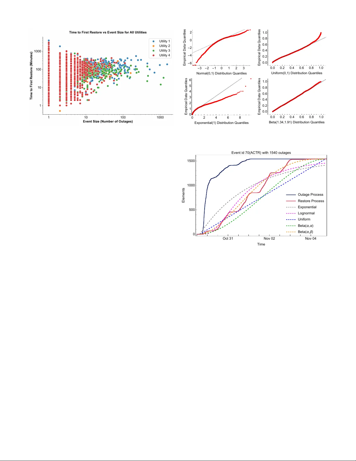
Author preprint March 2026 T ypical models of the distrib ution system restoration process Arslan Ahmad Iow a State Univ ersity arslan@iastate.edu Ian Dobson Iow a State Univ ersity dobson@iastate.edu Abstract —Accurate probabilistic modeling of the power system restoration pr ocess is essential for resilience planning, operational decision-making, and realistic simulation of resilience ev ents. In this work, we dev elop data-driven probabilistic models of the restoration process using outage data from four distribution utilities. W e decompose re storation into three components: normalized restore time progr ession, total r estoration duration, and the time to first restor e. The Beta distribution provides the best-pooled fit for restore time progr ession, and the Uniform distribution is a defensible, parsimonious approximation for many e vents. T otal duration is modeled as a heteroskedastic Lognormal process that scales superlinearly with event size. The time to first restore is well described by a Gamma model for moderate and large events. T ogether , these models provide an end-to-end stochastic model for Monte Carlo simulation, probabilistic duration forecasting, and resilience planning that moves beyond summary statistics, enabling uncertainty-aware decision support grounded in utility data. Index T erms —Resilience, distribution, restoration, pr obability I . I N T R O D U C T I O N Power restoration after an outage event is a complex time- ev olving process in which customers and components are progressiv ely restored as switching, repairs, and crew actions unfold. Y et more often, restoration is represented by a sin- gle summary statistic (e.g., an a verage restoration time) or by con venient assumptions (e.g., exponential repair), which obscures how restoration unfolds during an event and limits the modeling of restoration uncertainty in planning studies. Restoration process models matter because they (i) provide a probabilistic description of how restoration progresses in time rather than a single estimate, (ii) enable Monte Carlo simulations that require realistic restoration dynamics, and (iii) support restoration and resilience planning using data-driven models rather than ad hoc assumptions. In this paper , we use unscheduled outage data from four dis- tribution utilities to model the restoration process of resilience ev ents as three complementary components: (1) the normalized progression of restore times (restore process shape), (2) the total restoration duration, and (3) the time to first restore. Our emphasis is on identifying model classes that fit consistently Support from USA NSF grants 2153163 and 2429602, Argonne National Laboratory , and PSerc project S110 is gratefully acknowledged. across utilities under a common e vent definition, while also separating what is common from utility-specific aspects of restoration behavior . These models provide a practical foun- dation for simulation, benchmarking, and decision support, and they also allo w a direct comparison of distribution-system restoration process behavior with analogous models dev eloped for transmission-system resilience ev ents. The questions we answer in this work are: • What probabilistic model class best represents restoration times of distribution system outage events across multiple utilities, under a consistent ev ent definition, and with statistical evidence? • What is stable vs utility-specific about restoration-time behavior? • What do the “best-fit” probabilistic models enable that common practice (means/medians, or ad hoc assumptions like exponential) do not? I I . R E L AT E D W O R K Recent work on transmission resilience events has empha- sized e vent-based modeling and metrics that characterize how outages occur, progress, and reco ver over time, providing a useful analog for process-based modeling in distribution systems [1]. Complementary work has also shown how outage and restore process statistics can be extracted from utility data to compute events, processes, and metrics in distribution sys- tems [2]. In distribution systems, early statistical studies ana- lyzed outage restoration times and their dependence on factors such as time, consequence, and environment, establishing the value of empirical restoration-time modeling using utility data [3]. More recent approaches frame restoration time prediction using probabilistic models with cov ariates and operational factors; for example, accelerated failure-time and related sur - viv al models have been used to predict restoration time while accounting for spatial effects [4], and probabilistic restoration models ha ve been proposed for wide-area outages with links to repair resources and planning applications [5]. T an et al. [6] model the post-disaster repair and restoration process of distribution system outages as a scheduling problem. W ang et al. [7] use a sum of constants and double e xponentials to model ev ent restoration duration vs. number of outages after dividing the distribution system area into different weather zones. In contrast to existing work, this work focuses on utility- data-driven modeling of the r estoration pr ocess for events in distribution systems . I I I . U T I L I T Y D A TA W e use real-world data of unscheduled power outages from four different distribution utilities. Summary of the data is giv en in T able I. W e group indi vidual outages into events, where an ev ent is a set of outages that o verlap in time. W e calculate the restore process of each e vent as the cumulati ve number of outages restored during the ev ent. More details about the ev ents and processes are in [2], [8]. T ABLE I U T IL I T Y D AT A Utility-1 Utility-2 Utility-3 Utility-4 T ime period (years) 6 11 10 11 T otal outages 32278 6371 22371 13340 T otal events 5716 3832 7000 6485 # of events of size ≥ 30 132 13 71 17 I V . M E T H O D S Consider an event with n outages. Let r 1 , r 2 , ..., r n be the absolute restore times of outages sorted in ascending order , and ∆ r 1 , ∆ r 2 , ..., ∆ r n be the normalized restore times of outages relativ e to the first restore time, i.e., ∆ r i = ( r i − r 1 ) /D , with ∆ r i ∈ [0 , 1] , and D = r n − r 1 being the total duration of the restoration process. Let the time to first restore in the event be D r 1 = r 1 − o 1 , where o 1 is the start time of the first outage in the e vent. Our goal is to model the typical restoration process (1) by modeling D , D r 1 , and ∆ r i . The absolute restoration times can then be recov ered using r i = o 1 + D r 1 + D ∆ r i for i = 1 , 2 , 3 , ..., n (1) A. Modeling the Restore T imes Once the restoration process starts, the normalized restore times ∆ r i in an ev ent can be treated as an observed sample from a random variable R . W e w ant to estimate the distribution of R using the empirical data from many e vents. W e ev aluate the follo wing candidate distributions to find a distribution that best fits the observations of R : • Lognormal, Lognormal( µ, σ 2 ) • Exponential, Exp( λ ) , λ > 0 • Uniform, U (0 , 1) • Beta (with 1 parameter), Beta( α, α ) , α > 0 • Beta (with 2 parameters), Beta( α, β ) , α, β > 0 W e model the ev ent restore times in two dif ferent ways: 1) Global Model : W e normalize and combine the restore times of all the ev ents together to make a single set of observations and fit different candidate distributions to that set. The results are shown in Figs. 4 and 6. Estimated parameters for the best-fit of each distribution using this pooled-fit method are tabulated in T able III. 2) Individual Model : W e fit candidate distributions to the restore times of each individual e vent and ev aluate the Fig. 1. V ariation of Event Restoration Duration with Event Size (log-log scale). number of cases in which one candidate distribution giv es a better fit than the other . The results for these comparisons are given in T able IV. This method giv es us a range of fitted parameters for each distribution. The model parameters are estimated via MLE. Goodness-of- fit is ev aluated qualitativ ely using CDF and quantile plots and quantitativ ely using K olmogorov-Smirnov (KS) distance. For comparison between distributions, we use the AICc (2) and the Likelihood Ratio T est (for nested models only) to determine the best-fitting model while accounting for model comple xity . AICc = AIC + 2 k 2 + 2 k n − k − 1 , AIC = 2 k − 2ln[ ˆ L ] (2) Here k is the number of parameters in the model, n is the sample size, and ˆ L is the likelihood estimate. AICc adjusts AIC for small sample sizes. B. Modeling the Event Restoration Duration T o model the restoration duration D (in minutes) of ev ents, we consider strictly positive values; hence, only e vents with 2 or more outages are considered, as single-outage ev ents hav e a restoration duration of 0. W e start by analyzing the empirical distribution of restoration duration across all utilities and observe heavy tails (see Fig. 2). The slope magnitudes 1 of the distribution’ s CCDF tails on log-log plots range from 1.6 to 1.9, as indicated in T able II. For descriptiv e statistics, the distribution of restoration duration can be modeled using a spliced distrib ution where the tail is modeled using a Pareto distribution with parameter α p and cutof f values giv en in T able II, and the body of the distribution is modeled using a Lognormal distribution. Howe ver , a detailed model with a generativ e explanation is introduced below . Fig. 1 shows a scatter plot of ev ent restoration duration D and event size n on a log-log scale, clearly sho wing that, for each fixed ev ent size, restoration durations span orders 1 The slope magnitudes α p and the cutof f values D cutoff are determined automatically using Clauset’ s methods from [9] Empirical Distribution Fitted ( T a i l ) Distribution 1 10 100 1000 10 4 0.001 0.010 0.100 1 Restoration Duration D ( minutes ) Probability of Exceeding D Utility 1 D c u t o f f Empirical Distribution Fitted ( T a i l ) Distribution 0.01 0.10 1 10 100 1000 0.001 0.010 0.100 1 Restoration Duration D ( minutes ) Probability of Exceeding D Utility 2 D c u t o f f Empirical Distribution Fitted ( T a i l ) Distribution 0.1 1 10 100 1000 0.001 0.010 0.100 1 Restoration Duration D ( minutes ) Probability of Exceeding D Utility 3 D c u t o f f Empirical Distribution Fitted ( T a i l ) Distribution 0.01 0.10 1 10 100 1000 0.001 0.010 0.100 1 Restoration Duration D ( minutes ) Probability of Exceeding D Utility 4 D c u t o f f Fig. 2. Empirical CCDF of Ev ent Restoration Duration D of events with n ≥ 2 . The straight line shows a Pareto fit to the distribution tail starting at D cutoff . T ABLE II F I TT E D PA RA M E T ER S O F T H E R I G H T TA I L O F T H E D I S T RI B U TI O N O F E V EN T R E S TO R A T I O N D U RAT IO N Utility-1 Utility-2 Utility-3 Utility-4 D cutoff 360 280 330 429 Slope Magnitude α p 1.60 1.58 1.89 1.90 of magnitude across all utilities 2 . This approximately linear relationship between restoration duration and ev ent size on a log-log scale suggests power -law scaling, i.e., D ∝ n β . This means that the restoration duration is not generated by a single process; rather , it is a conditional outcome dependent on the underlying event size, which has two regimes: small and large ev ents. These regimes differ in causes (equipment failure vs. systematic vulnerability), response protocols (local repair vs. coordinated restoration and prioritization), and resource requirements (single crew vs multiple crews and mutual aid). Therefore, we model the ev ent restoration duration condition- ally on the ev ent size, explained as follows: D n = D | N = n ∼ Lognormal( µ ( n ) , σ 2 ( n )) (3) W e choose the lognormal distribution because of its positive support, right skewness (most ev ents resolve quickly), and heavy right tail (which captures rare but extreme v alues). W e model the mean structure E[ln( D n )] quadratically in ln( n ) as: µ ( n ) = ln( α 0 ) + β 1 ln( n ) + β 2 (ln( n )) 2 (4) The quadratic term in (4) allo ws the model to capture non- linear growth in restoration time and the saturation effects at very large e vent sizes. (A simple linear model was also tested, b ut the diagnostic plots sho wed systematic curv ature in µ ( n ) estimates, which is resolved by the quadratic model.) The intercept term α 0 is the baseline restoration duration, β 1 is the primary power law exponent (slope of linear trend on log-log plot), and β 2 is the quadratic coefficient to control the curvature. Since D n is lognormal, Median[ D n ] = e µ ( n ) = α 0 n β 1 n β 2 ln( n ) (5) which means that the median has a power -law relationship with e vent size, with its exponent changing with e vent size depending on the quadratic term exponent β 2 . 2 W e find that e vent size and restoration duration have a statistically significant (p-value < 0.05) positive correlation, with both Pearson and Spearman correlation coefficients exceeding 0.5. W e note in Fig. 1 that the variability in restoration dura- tion is not constant across ev ent sizes. In particular , relative variability appears to decrease with increasing event size. Assuming a constant variance (homoskedastic errors) in such a situation distorts both the tail behavior and uncertainty estimates. Therefore, we use a heteroskedastic variance model [10] to allow v ariance to decay exponentially with ev ent size: σ ( n ) = γ 0 + γ 1 e − δ n (6) The e xponential decay model (6) aligns with the change in variability sho wn in empirical data for all utilities in Fig. 1. It captures the rapid initial decay in variability via the decay rate parameter δ , allows additional variability γ 1 for small ev ents, and ensures a minimum asymptotic variability γ 0 . Th e coefficient of variation of D n can be calculated from the fact that it is a lognormal distribution as: CV = p e σ 2 − 1 (7) As n becomes large, (7) becomes p e γ 2 0 − 1 . The marginal distribution of D is obtained by integrating out N as: f D ( x ) = ∞ X n =2 f D n ( x ) · P ( N = n ) (8) = ∞ X n =2 P ( N = n ) xσ ( n ) √ 2 π exp( − (ln( x ) − µ ( n )) 2 2 σ 2 ( n ) ) (9) Since ev ent size N is discrete, the marginal distribution of D is a mixture of lognormals (9), naturally generating the heavy tails seen in Fig. 2. C. Modeling the T ime to F irst Restor e The time to first restore D r 1 = r 1 − o 1 of an event is the difference between the time when a restore happens for the first time r 1 in that ev ent and the start time o 1 of the first outage in the event. If we exclude outages restored by the automatic operation of the distribution protection system, the time to first restore comprises the cre w response time, trav el time, and the time to repair the faulted component. Unlike restoration durations, the empirical distributions of the time to first restore do not exhibit heavy tails 3 , except for utility 2. Also, the time to first restore does not sho w a statistically significant dependence on ev ent size; Fig. 3 visualizes the relationship. Howe ver , we observe two regimes 3 Slope magnitudes of the distribution tails on log-log plots are 2.76, 1.78, 4.40, 3.52 for utilities 1 to 4, respecti vely . Fig. 3. V ariation of Time T o First Restore with Event Size (log-log scale). with distinct variance trends: ev ents with fewer than ≈ 10 outages hav e significantly higher variability (1 minute to 2.7 days), which decreases with event size, whereas ev ents with ≈ 10 or more outages ha ve relati vely lower , more consistent variability (values centered around 100 minutes). Small events inherently ha ve higher v ariability because they may in volve simple fixes such as breaker resets or fuse replacements, as well as slower cases inv olving hard-to-find problems, remote locations, and complex diagnosis/repair . In contrast, the time to first restore for large e vents is relativ ely consistent because of defined procedures and protocols for responding to them. Continuous distributions, including Lognormal, Gamma, and W eibull, are tested, b ut none provided a statistically significant best fit for the time to first restore across all e vents. Therefore, e vents with at least 10 outages are selected, and the Gamma distribution is found to provide the best fit. For ev ents with fewer than 10 outages, the Lognormal and Gamma distributions giv e good fits for different utilities. V . R E S U L T S A N D D I S C U S S I O N A. Restore T imes - Global Model Fig. 4 shows the quantile plots of restore times of e vents in Utility 1 data. T o ensure a sufficient number of data points, we select events with at least 30 outages for restore times modeling. The results show that exponential and lognormal distributions are poor fits for the restore times, and the uni- form and beta distributions are good candidates; the uniform provides a poor fit in the tails, while the beta pro vides a good fit overall. T o substantiate this further , we look at the fits of these candidate distributions to the largest e vent in the data in Fig. 5. W e can see that, according to the lognormal model, the restore times slo w down significantly to wards the end of the ev ent, thereby failing to accurately model the restore process. The exponential distribution performs poorly in modeling both the start and the end of the restore process. The uniform distribution giv es a good fit in an av erage sense, whereas the restore times per the beta distribution nicely align with the empirical restore times. This is because the beta distribution - 3 - 2 - 1 0 1 2 3 - 6 - 4 - 2 0 2 Normal ( 0,1 ) Distribution Quantiles Empirical Data Quantiles 0.0 0.2 0.4 0.6 0.8 1.0 0.0 0.2 0.4 0.6 0.8 1.0 Uniform ( 0,1 ) Distribution Quantiles Empirical Data Quantiles 0 2 4 6 8 0 1 2 3 4 5 6 Exponential ( 1 ) Distribution Quantiles Empirical Data Quantiles 0.0 0.2 0.4 0.6 0.8 1.0 0.0 0.2 0.4 0.6 0.8 1.0 Beta ( 1.34,1.91 ) Distribution Quantiles Empirical Data Quantiles Fig. 4. Quantile–quantile plots comparing empirical normalized restore times ∆ r i (Utility 1, events with n ≥ 30 ) against candidate distributions. Outage Process Restore Process Exponential Lognormal Uniform Beta ( α , α ) Beta ( α , β ) Oct 31 Nov 02 Nov 04 0 500 1000 1500 T i m e Elements Event id 70 ( ACTR ) with 1540 outages Fig. 5. Example event restore process. Empirical outage and restore processes are compared with fitted restore time process models. fits the upper and lower tails of the data better (due to its in verted U shape, it giv es low probability in the tails). Based on these qualitative results, we rule out the lognormal and exponential distrib utions and proceed to test the beta and uni- form distributions quantitatively . W e note in passing that the beta distrib ution captures the diurnal patterns in which repairs sharply decrease at night in Fig. 5 only in an averaged sense. Fig. 6 shows the global models with uniform and beta distributions overlaid on the restore curves for all ev ents (with at least 30 outages) across the four utilities. T able III shows the best fit parameters along with goodness-of-fit metrics. A more negati ve AICc v alue indicates a better model, based on both the likelihood and the model comple xity . Based on these results, we conclude that the uniform distribution and the single-parameter beta distribution giv e comparable fits across all four cases, whereas the two-parameter beta distrib ution provides an overall superior fit, especially in tail regions. W e note that in the two-parameter beta model, β > α for all utilities, indicating that the restoration process is “front-loaded” with the probability density more concentrated at the beginning. F or example, the mean is α/ ( α + β ) ≈ 0 . 40 Restore Processes Beta ( 1.34,1.91 ) Beta ( 1.43,1.43 ) Uniform ( 0,1 ) 0.0 0.2 0.4 0.6 0.8 1.0 0.0 0.2 0.4 0.6 0.8 1.0 Proportion of T o t a l Restoration Duration Proportion of Outages Restored Utility 1 Restore Processes Beta ( 1.22,1.3 ) Beta ( 1.25,1.25 ) Uniform ( 0,1 ) 0.0 0.2 0.4 0.6 0.8 1.0 0.0 0.2 0.4 0.6 0.8 1.0 Proportion of T o t a l Restoration Duration Proportion of Outages Restored Utility 2 Restore Processes Beta ( 1.47,2.16 ) Beta ( 1.54,1.54 ) Uniform ( 0,1 ) 0.0 0.2 0.4 0.6 0.8 1.0 0.0 0.2 0.4 0.6 0.8 1.0 Proportion of T o t a l Restoration Duration Proportion of Outages Restored Utility 3 Restore Processes Beta ( 0.97,1.79 ) Beta ( 1.,1. ) Uniform ( 0,1 ) 0.0 0.2 0.4 0.6 0.8 1.0 0.0 0.2 0.4 0.6 0.8 1.0 Proportion of T o t a l Restoration Duration Proportion of Outages Restored Utility 4 Fig. 6. Global fitted models of restore times overlaid on the normalized empirical restore processes of e vents with size n ≥ 30 . T ABLE III R E SU LT S O F G L O BA L M O D EL S O F R E S TO R E T I ME S Utility-1 Utility-2 Utility-3 Utility-4 Standard Uniform KS Distance 0.16 0.07 0.19 0.28 Beta( α, α ) Parameters (1.4,1.4) (1.3,1.3) (1.5,1.5) (1.0,1.0) KS Distance 0.15 0.05 0.18 0.28 AICc -834 -19 -741 2 Beta( α, β ) Parameters (1.3,1.9) (1.2,1.3) (1.5,2.2) (1.0,1.8) KS Distance 0.01 0.05 0.02 0.07 AICc -2198 -20 -1863 -236 for utility 1, indicating that a significant portion of the components are restored within the first 40% of the total restoration duration window , while the remaining customers take disproportionately longer to fix. This implies that the repair rate decreases ov er time, likely because the easy fixes and automatic restorations are done first, leaving the complex ones for the tail end. B. Restore T imes - Individual Model The goodness-of-fit of the uniform and beta distrib utions is tested for the restore process of each event with 30 or more outages. Since these are nested distributions with increasing complexity , the likelihood ratio test is used instead of AICc to quantify the goodness-of-fit and its trade-off with complexity . The comparison of Uniform(0,1) and Beta( α, α ) in T able IV shows that the Beta distribution gives better AICc scores for all utilities. Howe ver , this better fit is due to an additional model parameter, as reflected in the Likelihood ratio test results (except for Utility 3). The LR T sho ws that, at the 0.05 significance le vel, in most cases the more comple x Beta( α, α ) model is unnecessary and the Uniform distribution is sufficient to model restore times for individual ev ents. T ABLE IV R E SU LT S O F I N D I VI D UA L M O D E LS O F R E S TO R E T I ME S , S H OW I N G F O R H OW M A N Y E V E NT S ( E X P RE S S E D A S P E R C EN TAG E O F T OTA L E V E NT S ) D I ST R I BU T I O N - A S C O R ED B E T TE R T H A N D I S TR I B UT I O N -B A S P E R D I FFE R E N T G O F C R I TE R I A Utility-1 Utility-2 Utility-3 Utility-4 Dist. A = Beta ( α, α ) , Dist. B = Uniform (0 , 1) KS Distance 67% 83% 77% 69% LR T 49% 42% 61% 31% Dist. A = Beta ( α, β ) , Dist. B = Beta ( α, α ) KS Distance 94% 92% 94% 100% LR T 55% 50% 63% 75% The LR T results in the lower half of T able IV suggest that the additional complexity of the Beta( α, β ) distrib ution is statistically significant as it fits the data better than the Beta( α, α ) distribution for more than 50% of the ev ents. C. Event Restoration Duration W e use maximum likelihood to estimate parameters of (3), (4), and (6). Given the data { ( x 1 , n 1 ) , ... ( x j , n j ) } and the parameter vector θ = ( α 0 , β 1 , β 2 , γ 0 , γ 1 , δ ) , we substitute the lognormal density of (3) in the following log-likelihood and maximize it over θ to estimate the parameters subjected to α 0 > 0 , γ 0 ≥ 0 , γ 1 ≥ 0 : l ( θ ) = j X i =1 ln f D n ( x i , n i ; θ ) (10) The estimated parameter values are tabulated in T able V. Utility 2 has the minimum baseline restoration duration α 0 for ev ents with 2 outages. All utilities ha ve β 1 > 1 , which means restoration duration scales superlinearly with e vent size. This suggests coordination and scalability challenges during large ev ents. The small, negati ve quadratic curv ature coefficient β 2 indicates that scaling becomes slightly less steep for large ev ents, and the marginal effect of additional outages on the restoration duration decreases. A lo wer γ 0 value is better as it gov erns the irreducible uncertainty for very large events. For example, for utility 4, the coefficient of v ariation (7) is 98%, indicating that very large ev ents exhibit high variability , which makes it more difficult to accurately estimate the restoration duration. Additional v ariability for small ev ents, in addition to the minimum variability γ 0 , is captured by γ 1 . Utility two has the smallest ratio of γ 1 /γ 0 = 1 . 6 , which means the small and large ev ents hav e similar variability in restoration duration. The variability decay rate δ is the largest for utility 4, which means that the small event v ariability is gone by n = 10 , i.e., 2 . 58 e − 0 . 65 × 10 ≈ 0 . T ABLE V P A R A M ET E R E S T IM ATE S O F T H E E V E N T R E S TO R A T I O N D U R A T I O N M O D E L Utility-1 Utility-2 Utility-3 Utility-4 α 0 (minutes) 26.14 14.03 17.04 20.16 β 1 1.45 1.35 1.60 1.92 β 2 -0.10 -0.05 -0.13 -0.20 γ 0 0.42 0.74 0.48 0.85 γ 1 1.89 1.18 1.29 2.58 δ 0.42 0.25 0.26 0.65 Empirical Distribution Fitted Distribution 5 10 50 100 500 10 - 4 0.001 0.010 0.100 1 T i m e to First Restore D r1 ( minutes ) Probability of Exceeding D r1 Utility 1 Empirical Distribution Fitted Distribution 20 50 100 200 0.005 0.010 0.050 0.100 0.500 1 T i m e to First Restore D r1 ( minutes ) Probability of Exceeding D r1 Utility 2 Empirical Distribution Fitted Distribution 5 10 50 100 0.001 0.010 0.100 1 T i m e to First Restore D r1 ( minutes ) Probability of Exceeding D r1 Utility 3 Empirical Distribution Fitted Distribution 5 10 50 100 0.01 0.05 0.10 0.50 1 T i m e to First Restore D r1 ( minutes ) Probability of Exceeding D r1 Utility 4 Fig. 7. Empirical CCDF (red) along with the fitted Gamma Distribution (blue) of Time T o First Restore of events with at least 10 outages. D. T ime to F irst Restor e Fig. 7 shows the empirical CCDF of the time to first restore for ev ents with at least 10 outages, along with the fitted Gamma distributions. Restricting to events with at least 10 outages reduces the high-variance regime visible in Fig. 3 and yields a more stable distrib ution across utilities. The fitted Gamma parameters are shown in T able VI. Utilities 1–3 hav e similar scale parameters ( θ ≈ 32 − 38 minutes) and moderate shape parameters ( k ≈ 2 . 4 − 3 . 4 ), which correspond to typical times to first restore, k θ , on the order of 1–2 hours. Utility 4 differs primarily in its variability: its fitted shape, k = 1 . 2 , implies substantially higher dispersion, and its larger scale ( θ ≈ 104 minutes) shifts the distribution to longer times. The coefficient of variation is 1 / √ k , which is lowest for Utility 1 (more consistent time to first restore) and highest for Utility 4 (least predictable time to first restore). T ABLE VI E S TI M A T E D PA RA M E T ER S O F T I ME T O F I RS T R E ST O R E ( M I N UT E S ) FI T Utility-1 Utility-2 Utility-3 Utility-4 Gamma Shape k 3.35 2.95 2.43 1.24 Gamma Scale θ 38.25 31.58 35.97 103.63 V I . C O N C L U S I O N This paper de velops data-dri ven probabilistic models for three components of the distribution-system restoration pro- cess: the normalized restore time progression, the total restora- tion duration, and the time to first restore. Using outage-e vent data from four utilities, we identify model classes that fit reliably across utilities. Beyond identifying best-fit distribution classes, the mod- els provide an operationally interpretable representation of restoration. In practice, once the outage process of an event ends, the utility soon kno ws the number of outages (the ev ent size). The conditional lognormal duration model (3) of restoration duration enables probabilistic forecasting of total restoration duration from e vent size, supporting early resource allocation, escalation decisions, and communication of expected do wntime. The restore-time process model for ∆ r i provides a typical “shape” of restoration progression within the e vent window , which is not captured by common practice that relies on means/medians or assumes exponential repair beha vior . By presenting the uniform distrib ution as a parsimonious alternati ve and the Beta( α, β ) distribution as the best-fit model for restore times of ev ents with n ≥ 30 , the results support selecting a model for low- and high-fidelity simulations that remains statistically defensible. These results on typical restore times in distribution systems differ from those in transmission systems [1], where a lognormal model is used rather than a uniform or beta distribution. T ime to first restore of moderate and lar ge ev ents shows a weaker dependence on event size than total restoration duration, but it exhibits a clear variance-regime change: small events hav e much higher v ariability than lar ge e vents. Utility-to-utility differences in the Gamma parameters indicate that the time to first restore is more utility-specific than the normalized restore-time process shape, which is comparativ ely stable across utilities. T ogether, these models provide a practical basis for realistic Monte Carlo simulation, benchmarking, and planning studies that require restoration dynamics considering uncertainty rather than single-point restoration estimates. R E F E R E N C E S [1] I. Dobson and S. Ekishev a, “How long is a resilience event in a transmission system?: Metrics and models driven by utility data, ” IEEE T rans. P ower Systems , vol. 39, no. 2, pp. 2814– 2826, 2024. [2] N. K. Carrington, I. Dobson, and Z. W ang, “Extracting re- silience metrics from distribution utility data using outage and restore process statistics, ” IEEE T rans. P ower Systems , vol. 36, no. 6, pp. 5814–5823, 2021. [3] M.-Y . Chow, L. T aylor , and M.-S. Chow, “Time of outage restoration analysis in distrib ution systems, ” IEEE T rans. P ower Delivery , vol. 11, no. 3, pp. 1652–1658, 1996. [4] T . B. Jamal and S. Hasan, “A generalized accelerated failure time model to predict restoration time from po wer outages, ” Intl. J. Disaster Risk Sci. , v ol. 14, no. 6, pp. 995–1010, 2023. [5] N. W illems et al., “Probabilistic restoration modeling of wide- area power outage, ” IEEE Access , vol. 12, pp. 184 431– 184 441, 2024. [6] Y . T an et al., “Scheduling post-disaster repairs in electricity distribution networks, ” IEEE T rans. P ower Systems , vol. 34, no. 4, pp. 2611–2621, 2019. [7] D. W ang et al., “Data-driven quantification and visualization of resilience metrics of po wer distrib ution systems, ” Scientific Reports , 2026. [8] A. Ahmad and I. Dobson, “Extracting resilience events from utility outage data based on overlapping times and locations, ” arXiv preprint , 2025, arXiv:2511.12685 [eess.SY] https://arxiv .org/abs/2511.12685. [9] A. Clauset, C. R. Shalizi, and M. E. J. Ne wman, “Power -law distributions in empirical data, ” SIAM Review , v ol. 51, no. 4, pp. 661–703, 2009. [10] R. J. Carroll, D. Ruppert, and L. A. Stefanski, Measurement err or in nonlinear models . CRC press, 1995, vol. 105.