Robust multi-scale leader-follower control of large multi-agent systems

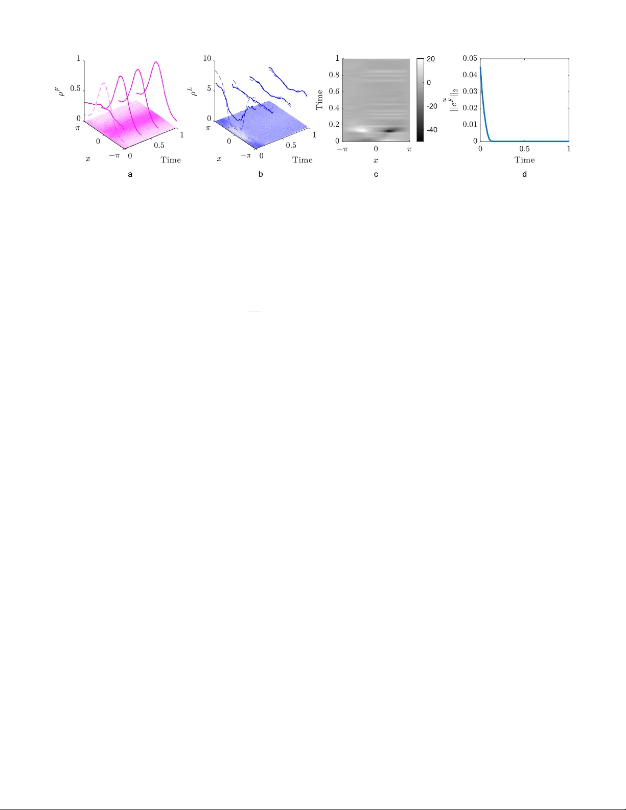
Rob ust multi-scale leader–f ollower contr ol of lar ge multi-agent systems Davide Salzano, Gian Carlo Maffettone and Mario di Bernardo Abstract — In many multi-agent systems of practical interest, such as traffic networks or cro wd e vacuation, control actions cannot be exerted on all agents. Instead, controllable lead- ers must indirectly steer uncontrolled f ollowers through local interactions. Existing r esults address either leader–follower density contr ol of simple, unperturbed multi-agent systems or rob ust density control of a single directly actuated population, but not their combination. W e bridge this gap by deriving a coupled continuum description for leaders and followers subject to unknown bounded perturbations, and designing a macroscopic feedback law that guarantees global asymptotic con vergence of the followers’ density to a desired distribution. The coupled stability of the leader–follower system is analyzed via singular perturbation theory , and an explicit lower bound on the leader-to-f ollower mass ratio required for feasibility is derived. Numerical simulations on heterogeneous biased random walkers validate our theor etical findings. I . I N T R O D U C T I O N Controlling the collectiv e beha vior of lar ge groups of inter - acting agents is a central challenge in domains ranging from traffic management [1] to crowd ev acuation [2] and swarm robotics [3]. When the number of agents is large, designing individual controllers becomes intractable [4]. Macroscopic approaches overcome this limitation by reformulating the control problem at the density lev el, describing collectiv e behavior through partial differential equations (PDEs) whose complexity is independent of the number of agents [5], [6]. A particularly effecti ve multi-scale approach [7] bridging microscopic (agent-lev el) and macroscopic (density-lev el) descriptions of multi-agent systems is continuification (or continuation) [8], [9]. In this approach, a continuum descrip- tion is derived from the agent-based model, the controller is designed at the PDE lev el, and the resulting control field is mapped back to agent-le vel inputs. The link between the two lev els of description relies on two operations: (i) a micr o-to- macr o bridge , which estimates the macroscopic density from the agents’ positions (e.g., via kernel density estimation), and (ii) a macr o-to-micr o bridge , which maps the control field computed at the PDE lev el back to individual agent inputs (e.g., via spatial sampling of the control field). This pipeline has been successfully applied to swarm robotics [10], traffic [11], and networks of lasers [12]. Davide Salzano and Gian Carlo Maffettone contributed equally to this work. Corresponding author: Mario di Bernardo. Davide Salzano and Mario di Bernardo are with the Department fo Electrical Engineering and Information T echnologies of the Univ ersity of Naples Federico II, Naples, Italy . ( davide.salzano@unina.it, mario.dibernardo@unina.it ) Gian Carlo Maffettone and Mario di Bernardo are with the Modeling and Engineering Risk and Complexity program of the Scuola Superiore Merid- ionale, Naples, Italy ( giancarlo.maffettone@unina.it ) In many scenarios of practical interest, howe ver , control actions cannot be exerted on all agents. In traffic networks, only autonomous vehicles are controllable [1]; in crowd ev acuation, only robotic guides can be actuated [2]. This motiv ates the leader–follower paradigm, where a population of controllable leaders steers uncontrolled followers through local interactions. A continuification-based solution to this problem was proposed in [13] and extended to shepherding [14] and bio-inspired plasticity [15]. A separate line of work [16] proposed a robust continuification strategy to counteract unknown bounded perturbations, b ut only for a single, directly actuated population. The combination of these two directions, rob ustness and indirect actuation, poses challenges that neither framew ork addresses when operating in isolation. This gap is tackled in this work. When both populations are subject to unknown bounded perturbations, the followers’ conv ergence depends on the ability of the leaders to track a time-varying reference density , generated by the robust controller . This couples the two populations’ dynamics in a way that requires a dedicated stability analysis. In this paper , we address this problem by deriving a coupled continuum description for leaders and followers subject to bounded perturbations, and designing a macroscopic feedback control law that guarantees global asymptotic con ver gence of the followers’ density to a desired distribution. W e deriv e an explicit lower bound on the leader mass required for the control problem to admit a solution, and, using singular perturbation theory , we analyze the stability of the coupled system. Numerical simulations on heterogeneous biased random walkers v alidate our findings and illustrate robustness to increasing levels of population heterogeneity and finite populations size. I I . M A T H E M A T I C A L M O D E L I N G A. Microscopic model W e consider two populations of interacting agents, leaders and follo wers, ev olving on the unit circle Ω = [ − π , π ] . The dynamics of N L leaders and N F followers are d x L i ( t ) =  u i ( t ) + h i ( t , X L ( t ))  d t , i = 1 , . . . , N L , (1a) d x F i ( t ) = " N L ∑ j = 1 f ( { x F i ( t ) , x L j ( t ) } π ) + g i ( t , X F ( t )) # d t + √ 2 D d W i ( t ) , i = 1 , . . . , N F , (1b) where x L i , x F i ∈ Ω are the states of the i -th leader and follo wer, X L ∈ Ω N L and X F ∈ Ω N F are the stack vectors containing the states of all leaders and follo wers, h i : R × Ω N L → R and g i : R × Ω N F → R are internal dynamics characterizing each Follo wers control Leaders’ controller Macro-to-micro bridge Multi-agent dynamics Micro-to-macro bridge ¯ ρ F − e F ¯ ρ L − e L u ( x , t ) u i x i ρ F ρ L ρ F Fig. 1. Block diagram of the multi-scale leader-follower control architecture. An outer loop regulates the followers’ density by comparing the reference ¯ ρ F with the estimated density ρ F , generating a reference density ¯ ρ L for the leaders. An inner loop tracks this reference, producing the macroscopic control field u ( x , t ) . The macr o-to-micro bridge maps u ( x , t ) to individual leader inputs u i via spatial sampling. The multi-agent dynamics produce leader and follower positions x i , which the micr o-to-macro bridge conv erts back to estimated densities ρ L and ρ F via density estimation, closing both feedback loops. population, u i ∈ R is the control input acting on leaders, and W i is a standard W iener process with dif fusion coefficient D . The interaction kernel f : Ω → R is the odd kernel [13] f ( x ) = sgn ( x ) e 2 π /ℓ − 1 h e 2 π −| x | ℓ − e | x | ℓ i . (2) It describes ho w leaders influence followers, with ℓ being the characteristic interaction length. The internal dynamics h i and g i are unknown and uniformly bounded, that is, | h i ( t , X L ( t )) | < r , ∀ i ∈ 1 , . . . , N L , ∀ t ∈ R ≥ 0 , (3a) | g i ( t , X F ( t )) | < k , ∀ i ∈ 1 , . . . , N F , ∀ t ∈ R ≥ 0 , (3b) with r , k ≥ 0. B. Macroscopic model Since the perturbations are unknown but bounded, we ap- ply the comparison principle to construct bounding systems that replace h i and g i with their worst-case v alues ± r and ± k [16]. T aking the mean-field limit of the bounding system of both populations yields the coupled PDEs ρ L t ( x , t ) +  ρ L ( x , t )( u ( x , t ) ± r )  x = 0 , (4a) ρ F t ( x , t ) +  ρ F ( x , t )( v F L ( x , t ) ± k )  x = D ρ F xx ( x , t ) , (4b) where x ∈ Ω , the ± signs correspond to the upper and lower bounding systems, and v F L ( x , t ) = Z Ω f ( { x , y } π ) ρ L ( y , t ) d y = ( f ∗ ρ L )( x , t ) . (5) A control law that stabilizes both bounding systems guaran- tees stabilization of the original system (1) for an y realization of the perturbations. Model (4) is complemented with initial conditions and periodic boundary conditions ensuring mass conservation  Z Ω ρ i ( x , t ) d x  t = M i t ( t ) = 0 , i = L , F , (6) where M L , M F are the mass of leaders and followers. C. Problem statement Giv en a time-in variant desired density profile ¯ ρ F : Ω → R > 0 , such that R Ω ¯ ρ F d x = M F , we seek for a periodic u in (4) such that lim t → ∞ ∥ e F ( · , t ) ∥ 2 = 0 , (7) where e F = ¯ ρ F − ρ F and ∥ · ∥ 2 is the L 2 ( Ω ) -norm. I I I . C O N T R O L D E S I G N W e design a control field u : Ω × R → R that guarantees asymptotic conv ergence of the control error . The strategy proceeds in two stages. First, we treat the velocity field v F L as a free design variable and deri ve stability conditions for the followers’ dynamics. Then, we constrain v F L = f ∗ ρ L to recov er a physically meaningful reference density for the leaders via decon volution, and we construct a feedback law steering the leaders towards such a desired density . The resulting coupled system is analyzed using singular perturbation theory [17]. Our strate gy is complemented with micro-to-macro and macro-to-micro bridges as illustrated in Fig. 1: the micro-to-macro bridge consists in a density estimation procedure, while the macro-to-micro bridge is implemented via a spatial sampling. A. F ollower s contr ol design As mentioned abo ve, to study the stability properties of the follower population, we assume it is possible to arbitrarily choose their drift. Under this assumption, we choose v F L as the con ve x combination v F L ( x , t ) = [ 1 − α ( t )] v F F ( x ) + α ( t ) v F B ( x , t ) , (8) where α : R ≥ 0 → [ 0 , 1 ] is a design function, v F F is a feedforward action and v F B is a feedback correction. More precisely , v F F is chosen as in [13], that is v F F ( x ) = D ¯ ρ F x ( x ) ¯ ρ F ( x ) . (9) This choice ensures that, in absence of any disturbance and unmodeled dynamics, when v F B = 0, the followers displace according to the desired density profile if ∥ g 1 ∥ ∞ < 2, with g 1 ( x ) =  ¯ ρ F x ( x ) ¯ ρ F ( x )  x . (10) For more details on this result, see [13]. Theor em 1: W e choose v F L in (8), with v F B such that  ρ F ( x , t ) v F B ( x , t )  x = q F ( x , t ) . (11) Here q F ( x , t ) = − k F p e F ( x , t ) − k F s ( t ) sign  e F ( x , t )  + β ( t ) , (12) where β is a bounded function of time. If ∥ g 1 ∥ ∞ < 2, k F p > 0, k F s ( t ) > α ( t ) D ∥ ¯ ρ F xx ( · ) ∥ ∞ + k ∥ ¯ ρ F x ( · ) ∥ ∞ α ( t ) , (13) then e F globally asymptotically con verges to 0 in L 2 ( Ω ) , ∀ α ∈ ( 0 , 1 ] . Pr oof: W e substitute (8) with (11) into (4b), yielding (dropping dependence from space and time for compactness) ρ F t + ( 1 − α ) D  ρ F ¯ ρ F xx ¯ ρ F  x + α q F ± k ρ F x = D ρ F xx . (14) Recalling that e F = ¯ ρ F − ρ F , we can rephrase (14) in terms of the error function, resulting in e F t = − α D ¯ ρ F xx − ( 1 − α ) D  e F ∇ ¯ ρ F ¯ ρ F  x + α q F ± k ¯ ρ F x ∓ ke F x + De F xx . (15) Initial and periodic boundary conditions of the error system can be recovered from those of (4). W e introduce the L yapunov functional V F = 1 2 ∥ e F ∥ 2 2 and compute its time deriv ativ e V F t = Z Ω e F e F t d x = − D α Z Ω e F ¯ ρ F xx d x + D Z Ω e F e F xx d x − ( 1 − α ) D Z Ω e F  e F ¯ ρ F x ¯ ρ F  x d x ± k Z Ω e F ¯ ρ F x d x ∓ k Z Ω e F e F x d x + α Z Ω e F q F d x , (16) where we used (15). Let us establish the following relations: D Z Ω e F e F xx d x = − D Z Ω  e F x  2 d x = − D ∥ e F x ∥ 2 2 ≤ − 2 D V F , (17a) α D     Z Ω e F ¯ ρ F xx d x     ≤ α D ∥ e F ¯ ρ F xx ∥ 1 ≤ α D ∥ e F ∥ 1 ∥ ¯ ρ F xx ∥ ∞ , (17b) − ( 1 − α ) D Z Ω e F  e F ¯ ρ F x ¯ ρ F  x d x = ( 1 − α ) D 2 Z Ω  ( e F ) 2  x ¯ ρ F x ¯ ρ F d x = − ( 1 − α ) D 2 Z Ω ( e F ) 2 g 1 d x ≤ ( 1 − α ) D 2     Z Ω ( e F ) 2 g 1 d x     ≤ ( 1 − α ) D 2 ∥ e F e F g 1 ∥ 1 ≤ ( 1 − α ) D ∥ g 1 ∥ ∞ V F , (17c) ± k Z Ω e F ¯ ρ F x d x ≤ k     Z Ω e F ¯ ρ F x d x     ≤ k ∥ e F ¯ ρ F x ∥ 1 ≤ k ∥ ¯ ρ F x ∥ ∞ ∥ e F ∥ 1 (17d) ± k Z Ω e F e F x d x = ± k 2 Z Ω  ( e F ) 2  x d x = ± k 2  ( e F ) 2  π − π = 0 , (17e) in which we used integration by parts (boundary terms v anish due to boundary conditions), Poincar ` e-W irtinger [18] and H ¨ older inequality [19], and the identity [( e F ) 2 ] x = 2 e F e F x . Note that the last relation is true due to periodic boundaries, and the function g 1 is defined in (10). Applying the bounds in (17) to (16) yields V F t ≤ [ D ( 1 − α ) ∥ g 1 ∥ ∞ − 2 D ] V F +  α D ∥ ¯ ρ F xx ∥ ∞ + k ∥ ¯ ρ F x ∥ ∞  Z Ω | e F | d x + α Z Ω e F q F d x . (18) Substituting the expression of q F in (12) into (18) yields V F t ≤  D ( 1 − α ) ∥ g 1 ∥ ∞ − 2 D − α k F p  V F +  α D ∥ ¯ ρ F xx ∥ ∞ + k ∥ ¯ ρ F x ∥ ∞ − α k F s  Z Ω | e F | d x . (19) Under the theorem hypotheses, the right-hand side is negativ e proving the claim. Remark 1: The function β ( t ) in (12) does not play any role for stability properties. Howe ver , it needs to be chosen to ensure the control flux fulfills boundary conditions; see [16, Sec. VI.4] Remark 2: The presence of discontinuous terms in (12) and (31) (i.e., sign ( · ) ) implies that the solutions of the closed- loop PDEs (4) must be interpreted in a weak sense. Existence of such solutions under discontinuous flux is guaranteed by [20, Definition 1]; see also [16, Remark 2] for a detailed discussion in our setting. B. Deconvolution and choice of α ( t ) Since v F L = f ∗ ρ L , we now recov er a reference density ¯ ρ L for the leaders that produces v F L as defined in (8). Using the kernel (2), any velocity field v can be deconv olved to retriev e the generating density as ρ ( x , t ) = v x ( x , t ) 2 − 1 2 ℓ 2 Z v ( x , t ) d x + I ( t ) , (20) where I : R → R is an arbitrary function of time; see [13, App. B]. Since v F L is a con ve x combination of feedforward and feedback contributions and con volution is linear, the generating density takes the form ¯ ρ L ( x , t ) = [ 1 − α ( t )] ρ F F ( x ) + α ( t ) ρ F B ( x , t ) + G ( t ) , (21) where G : R ≥ 0 → R is an arbitrary function of time, and ρ F F , ρ F B are obtained by deconv olving v F F and v F B , respectively . As noted in [13], the decon volution operation does not guarantee that the obtained densities are physically meaningful (i.e. that they are non negati ve and that they sum to the mass of av ailable leaders). T o guarantee pos- itiv eness, we choose G ( t ) = − ( 1 − α ( t )) min x ( ρ F F ( x , t )) − α ( t ) min x ( ρ F B ( x , t )) + C ( t ) that guarantees ¯ ρ L ( x , t ) > 0 for any C ( t ) ≥ 0. Instead, to guarantee that the density integrates to the available mass of leaders M L , we choose suitable values of α and C . Specifically , it holds that Z Ω ¯ ρ L d x = [ 1 − α ] M F F + α M F B + | Ω | C , (22) where M F B = R Ω ρ F B d x and we recall M F F = R Ω ρ F F d x . W e need to choose α that guarantees [ 1 − α ] M F F + α M F B ( t ) + | Ω | C ≤ M L . (23) This allows choosing a non-neg ativ e C such that R Ω ¯ ρ L d x = M L . Note that (23) is equiv alent to α [ M F B − M F F ] + | Ω | C ≤ M L − M F F . (24) Assuming M L − M F F > 0, which is guaranteed under the feasibility conditions reported in [13], we choose α = ( M L − M F F M F B ( t ) − M F F if M F B ( t ) > M F F 1 , otherwise (25) and C = max  0 , M L − M F F − α ( M F B − M F F )  . (26) This ensures that ¯ ρ L is a physically meaningful density . C. Minimum leader mass for feasibility The choice of α in (25) maximizes the feedback weight giv en the available leader mass, but can violate (13). T o guarantee simultaneously a feasible ¯ ρ L and global asymptotic stability , we combine (13) and (25), yielding k ∥ ¯ ρ F x ∥ ∞ k F s − D ∥ ¯ ρ F xx ∥ ∞ ≤ M L − M F F M F B − M F F , if M F B > M F F (27a) k ∥ ¯ ρ F x ∥ ∞ k F s − D ∥ ¯ ρ F xx ∥ ∞ ≤ 1 , if M F B ≤ M F F . (27b) When M F B ≤ M F F , the action is purely feedback and (27b) reduces to k F s > D ∥ ¯ ρ F xx ∥ ∞ + k ∥ ¯ ρ F x ∥ ∞ . When M F B > M F F , inequality (27a) provides an explicit lo wer bound on the leader mass M L for the control problem to admit a solution M L ≥ sup t ∈ R ≥ 0  M F F + k ∥ ¯ ρ F x ∥ ∞ ( M F B − M F F ) k F s − D ∥ ¯ ρ F xx ∥ ∞  . (28) Since q F is linear in k F s and M F B maps to q F through linear operators, we write M F B = k F s M s + M , where M s and M are the mass contributions from the switching term − sign ( e ) and the remaining terms in q F , respectiv ely . In the limit k F s → ∞ , the minimum leader mass becomes M L ≥ sup t ∈ R ≥ 0  M F F + k ∥ ¯ ρ F x ∥ ∞ M s  (29) Remark 3: The lo wer bound (29) can be interpreted as a herdability condition [21] in a continuum setting, as it quantifies the minimum leader resources required to steer the follo wer population to a prescribed density . Additionally , condition (29) shows that this requirement grows linearly with the perturbation bound k . D. Leaders’ control W e choose u in (4a) such that leaders track the time- varying reference ¯ ρ L in (21) with α and C as in Sec. III-B. T o reject the bounded perturbations on the leaders, we select u such that  ρ L ( x , t ) u ( x , t )  x = q L ( x , t ) , (30) where q L ( x , t ) = − k L p e L ( x , t ) − k L s sign  e L ( x , t )  + ¯ ρ L t ( x , t ) + δ ( t ) , (31) e L = ¯ ρ L − ρ L , k L p ( t ) > 0, k L s > k ∥ ¯ ρ L ( · , t ) ∥ ∞ , and δ is chosen to satisfy boundary conditions. This control law guarantees global exponential stability in L 2 ( Ω ) , since we can write V L t ( t ) ≤ − k L p V L ( t ) , (32) where V L = 1 2 ∥ e L ∥ 2 2 ; the proof follows from [16, Theorem 1]. E. Coupled stability analysis The analysis in Secs. III-A and III-D treats leaders and followers independently . W e no w account for the coupling: the followers’ L yapunov deriv ative depends on the leaders’ tracking error e L through the interaction kernel. Specifically , the L 2 ( Ω ) norms of the density errors are given by V F t ≤  D ( 1 − α ) ∥ g 1 ∥ ∞ − 2 D − α k F p  V F − Z Ω e F  ¯ ρ F ( f ∗ e L )  x d x − Z Ω e F  ρ F ( f ∗ e L )  x d x , (33a) V L t ≤ − k L p V L . (33b) The two additional terms in (33a) capture the effect of the leaders’ transient on the followers. W e bound them as     Z Ω e F  ¯ ρ F ( f ∗ e L )  x d x     ≤ J √ V F √ V L , (34a)     Z Ω e F  e F ( f ∗ e L )  x d x     ≤ S V F √ V L , (34b) where J = 2 ∥ ¯ ρ F x ∥ 2 ∥ f ∥ 2 + 2 ∥ ¯ ρ F ∥ 2 ∥ f x ∥ 2 , (35a) S = √ 2 ∥ f ∥ 2 . (35b) T o recover such bounds we proceed similarly to (17) bound- ing con volutions with Y oung’ s inequality [19]. Theor em 2: Consider the leader–follower system (4) with the followers’ control law (8)–(12) and the leaders’ control law (31), under the hypotheses of Theorem 1. If k L p is chosen suf ficiently large, then the followers’ density error e F globally asymptotically con ver ges to zero in L 2 ( Ω ) . Pr oof: Substituting the bounds (34) into (33a) yields V F t ≤  D ( 1 − α ) ∥ g 1 ∥ ∞ − 2 D − α k F p  V F + J √ V F √ V L + S V F √ V L . (36) Letting ε = 1 / k L p , the coupled system becomes V F t =  D ( 1 − α ) ∥ g 1 ∥ ∞ − 2 D − α k F p  V F + J √ V F √ V L + S V F √ V L , (37a) ε V L t = − V L , (37b) where, with an abuse of notation, V F and V L denote the v ari- ables of the bounding system. This is a singularly perturbed system in standard form [17]. The boundary-layer system (37b) has a unique globally exponentially stable equilibrium at V L = 0. Substituting it into the reduced system (37a) yields V F t =  D ( 1 − α ) ∥ g 1 ∥ ∞ − 2 D − α k F p  V F , which is globally asymptotically stable under the hypotheses of Theorem 1. By Tikhono v’ s theorem, for sufficiently small ε (equiv alently , sufficiently large k L p ), the trajectories of the full system con ver ge to those of the reduced system, completing the proof. Remark 4: The timescale separation requires k L p to be large relativ e to the followers’ con ver gence rate. Since V L decays as e − k L p t and the coupling enters through √ V L , a practical guideline is k L p ≫ 2 ( 2 D + α k F p ) , ensuring that the leaders’ transient is negligible on the followers’ timescale. Fig. 2. Control of biased random walkers moving on a ring . a . Evolution in time and space of all the followers in the ensemble (x- and y-axes). On the z-axis the estimated (solid) and desired (dashed) densities are displayed in four representative time instants. b . Evolution in time and space of all the leaders in the ensemble (x- and y-axes). On the z-axis the estimated (solid) and desired (dashed) densities are displayed in four representativ e time instants. c . Evolution in time and space of the velocity field u ( x , t ) generated by the controller and used to steer the leaders tow ards their desired density . d . Evolution of the L 2 ( Ω ) norm of the followers control error in time. I V . N U M E R I C A L V A L I D A T I O N For validation, we control an ensemble of biased random walkers with heterogeneous drifts on the unit circle d x F i = b i + N L ∑ j = 1 f ( { x F i ( t ) , x L j ( t ) } π ) ! d t + √ 2 D d W i (38) for i = 1 , . . . , N F , with N F = 5000. With respect to (1), g i ( x i ( t )) = b i is a constant drift drawn from U ([ − 2 , 2 ]) . W e set D = 0 . 1, ℓ = π , and assign each follower a mass 1 / N F , yielding M F = 1. Leaders are unperturbed single integrators, d x L i ( t ) = u i ( t ) d t , (39) for i = 1 , . . . , N L , with N L = 5000 and mass 30 / N L each, so that M L = 30. The target follower density is the V on Mises distribution ¯ ρ F = e ( κ cos ( x − µ )) with µ = 0, κ = 1. Since leaders are unperturbed, we set k = 1, r = 0, and choose k F s = 5 ( D ∥ ¯ ρ F xx ∥ ∞ + k ∥ ¯ ρ F x ∥ ∞ ) , k F p = 2, k L s = 0 . 1. The choice k L p = 50 enforces the timescale separation required by Theorem 2. The deriv ati ve ¯ ρ L t is approximated via backward differences on an exponential moving average of ¯ ρ L . T o suppress chattering, we regularize sign ( x ) as tanh ( η x ) with η = 10 2 . The densities ρ F and ρ L are estimated from agents’ positions using a micro-to-macro bridge: a normal- ized histogram on a grid of 150 points, filtered with a Gaussian kernel of length of approximately π / 30. The same filter is applied to ¯ ρ L to reduce numerical instabilities. The macro-to-micro bridge assigns each leader u i ( t ) = u ( x L i , t ) by spatial sampling. Simulations are run in MA TLAB using forward Euler (leaders, step 2 · 10 − 6 ) and Euler–Maruyama (followers, step 2 · 10 − 4 ). Fig. 2a sho ws that the followers con verge to the desired density in approximately 0 . 2 time units. Fig. 2b displays the leaders tracking the time-v arying reference ¯ ρ L ; the residual error is due to the regularization of the switching action and the numerical approximation of ¯ ρ L t . The control field is shown in Fig. 2c. ∥ e F ∥ 2 decreases monotonically to zero (Fig. 2d). The numerically computed minimum leader mass is M L ≥ 17, which is satisfied with M L = 30. T o assess rob ustness to increasing heterogeneity , we re- peated the simulations with b i ∼ U ([ − B , B ]) for B ∈ [ 2 , 20 ] , setting k F s = 5 ( D ∥ ¯ ρ F xx ∥ ∞ + B ∥ ¯ ρ F x ∥ ∞ ) and k F p = 2. As shown in Fig. 3a, the steady-state error remains zero as long as (29) is satisfied. When heterogeneity makes the minimum mass required higher than the av ailable mass, asymptotic con ver - gence is lost and the error grows with B . A representative case with B = 20 is shown in Fig. 3b, where leaders fail to steer followers to the target profile. A. Finite population effects Our architecture rests on a mean-field assumption that requires populations to be suf ficiently large. T o quantify the minimum population sizes for the micro-to-macro bridges to operate reliably , we simulated system (4) under the control law of Sec. III, using the same scheme and gains as in Fig. 2. The total masses are held fixed at M F = 1 and M L = 30 across all runs, so that varying N L or N F does not change the leader-to-follo wer mass ratio. N L ( N F ) were sampled in the interval [ 10 , 5000 ] using 30 samples equally spaced in logarithmic scale. Fig. 4 (orange line) shows the residual error as a function of the number of leaders N L , with the number of follo wers fixed at N F = 1000. A clear threshold emerges: below the critical v alue of N L ≈ 130, the leaders are too sparse for the macro-to-micro bridge to faithfully reproduce the control field, and the error consistently settles at a high value. Abov e this threshold, the error norm on the followers density decreases below 10 − 2 , identifying this value as the minimum amount of leaders required to correctly reconstruct densities from agents’ positions. Con versely , Fig. 4 (blue line) reports the error as a function of N F with N L = 1000 fixed. W e find that, ev en in the presence of a large number of leaders, a minimum number of followers ( N F ≈ 400) is required to reduce the norm of the error to v alues less than 10 − 2 . These observations are in line with the herdability conditions recently reported in [21]. V . C O N C L U S I O N S W e proposed a robust multi-scale leader -follower control strategy for large-scale multi-agent systems in which both populations can be affected by unknown bounded pertur- bations. The control architecture consists of a macroscopic Fig. 3. Robustness to heter ogeneity . a . L 2 ( Ω ) norm of the followers control error for increasing heterogeneity in the follower population. The red shaded area represents the conditions where (29) is not satisfied. T = 1 is the terminal instant of the simulation. b . Evolution in time and space of all the followers in the ensemble when b i ∼ U ([ − 20 , 20 ]) . On the z axis the estimated (solid) and desired (dashed) densities are displayed in four representativ e time instants. Fig. 4. Effects of finite population size . L 2 ( Ω ) norm of the followers control error when (a) varying the number of leaders N L ∈ [ 10 , 5000 ] when N F = 1000, and (b) varying the number of followers N F ∈ [ 10 , 5000 ] when N L = 1000 (vertical dashed lines denote the threshold above which the error norm is belo w 10 − 2 ). T = 1 . 5 is the terminal instant of the simulation. N L ( N F ) were sampled in the interval with [ 10 , 5000 ] using 30 samples equally spaced in logarithmic scale. feedback law that guarantees global asymptotic con vergence of the followers’ density to a prescribed profile, and maps it to individual leader inputs via spatial sampling. A minimum leader mass and a timescale separation between leaders and followers dynamics are required to guarantee global asymptotic stability of the followers closed loop dynamics. Numerical v alidation on heterogeneous biased random walk- ers confirms the theoretical findings and illustrates rob ustness to increasing levels of population heterogeneity . Furthermore, we study the effects of a finite population sizes on the performance of the control architecture. Current limitations include the mean-field assumption ( N F , N L → ∞ ), the assumption of having global kno wledge of both density profiles (centralized control), and the restriction to one-dimensional domains. Future work will address con- ver gence guarantees in the presence of finite population sizes, distributed density estimation algorithms [22], and higher - dimensional settings. A C K N O W L E D G E M E N T S AI tools were used for language editing. All technical content is entirely the authors’ own. R E F E R E N C E S [1] S. Siri, C. Pasquale, S. Sacone, and A. Ferrara, “Freeway traffic control: A survey , ” Automatica , vol. 130, p. 109655, 2021. [2] M. Zhou, H. Dong, P . A. Ioannou, Y . Zhao, and F .-Y . W ang, “Guided crowd ev acuation: approaches and challenges, ” IEEE/CAA Journal of Automatica Sinica , vol. 6, no. 5, pp. 1081–1094, 2019. [3] M. Dorigo, G. Theraulaz, and V . Trianni, “Swarm robotics: Past, present, and future [point of view], ” Proceedings of the IEEE , vol. 109, no. 7, pp. 1152–1165, 2021. [4] R. M. D’Souza, M. Di Bernardo, and Y .-Y . Liu, “Controlling complex networks with complex nodes, ” Natur e Reviews Physics , vol. 5, no. 4, pp. 250–262, 2023. [5] C. Sinigaglia, A. Manzoni, and F . Braghin, “Density control of large- scale particles swarm through PDE-constrained optimization, ” IEEE T ransactions on Robotics , vol. 38, no. 6, pp. 3530–3549, 2022. [6] K. Elamvazhuthi and S. Berman, “Density stabilization strategies for nonholonomic agents on compact manifolds, ” IEEE T ransactions on Automatic Contr ol , vol. 69, no. 3, pp. 1448–1463, 2024. [7] M. di Bernardo, “Multi-scale control of large agent populations: From density dynamics to indi vidual actuation, ” , 2026. [8] D. Nikitin, C. Canudas-de W it, and P . Frasca, “ A continuation method for large-scale modeling and control: from ODEs to PDE, a round trip, ” IEEE T ransactions on Automatic Contr ol , vol. 67, no. 10, pp. 5118–5133, 2022. [9] G. C. Maffettone, A. Boldini, M. Di Bernardo, and M. Porfiri, “Continuification control of large-scale multiagent systems in a ring, ” IEEE Control Systems Letters , vol. 7, pp. 841–846, 2023. [10] G. C. Maffettone, L. Liguori, E. Palermo, M. Di Bernardo, and M. Por - firi, “Mixed reality environment and high-dimensional continuification control for swarm robotics, ” IEEE T ransactions on Contr ol Systems T echnology , 2024. [11] S. Fueyo and C. C. de Wit, “ A continuation-based control strategy for stabilizing second-order macroscopic traffic flo w on circular roads, ” Pr oceedings of the 64th IEEE Confer ence on Decision and Control , 2025. [12] D. Nikitin, C. Canudas-de Wit, and P . Frasca, “Boundary control for stabilization of large-scale networks through the continuation method, ” Pr oceedings of the 60th IEEE Conference on Decision and Control (CDC) , pp. 4792–4797, 2021. [13] G. C. Maffettone, A. Boldini, M. Porfiri, and M. di Bernardo, “Leader- follower density control of spatial dynamics in large-scale multi-agent systems, ” IEEE T ransactions on Automatic Contr ol , vol. 70, no. 10, pp. 6783–6798, 2025. [14] B. Di Lorenzo, G. C. Maffettone, and M. Di Bernardo, “ A continuification-based control solution for large-scale shepherding, ” Eur opean Journal of Contr ol , vol. 86, p. 101324, 2025. [15] G. C. Maffettone, A. Boldini, M. di Bernardo, and M. Porfiri, “Bio-inspired density control of multi-agent swarms leader-follower plasticity , ” Automatica (in pr ess) , 2026. [16] G. C. Maffettone, D. Salzano, and M. di Bernardo, “Rob ust macro- scopic density control of heterogeneous multi-agent systems, ” arXiv pr eprint arXiv:2602.09695 , 2026. [17] P . Kok otovi ´ c, H. K. Khalil, and J. O’ reilly , Singular perturbation methods in contr ol: analysis and design . SIAM, 1999. [18] J. Heinonen, Lectur es on analysis on metric spaces . Springer , 2001. [19] S. Axler , Measure , integration & r eal analysis . Springer Nature, 2020. [20] A. Cristof aro, “Robust distributed control of quasilinear reaction– diffusion equations via infinite-dimensional sliding modes, ” Automat- ica , vol. 104, pp. 165–172, 2019. [21] A. Lama and M. di Bernardo, “Shepherding and herdability in complex multiagent systems, ” Physical Revie w Research , vol. 6, no. 3, p. L032012, 2024. [22] B. Di Lorenzo, G. C. Maffettone, and M. di Bernardo, “Decentralized continuification control of multi-agent systems via distributed density estimation, ” IEEE Contr ol Systems Letters , vol. 9, pp. 1580–1585, 2025.