Consensus in Multi-Agent Systems with Uniform and Nonuniform Communication Delays

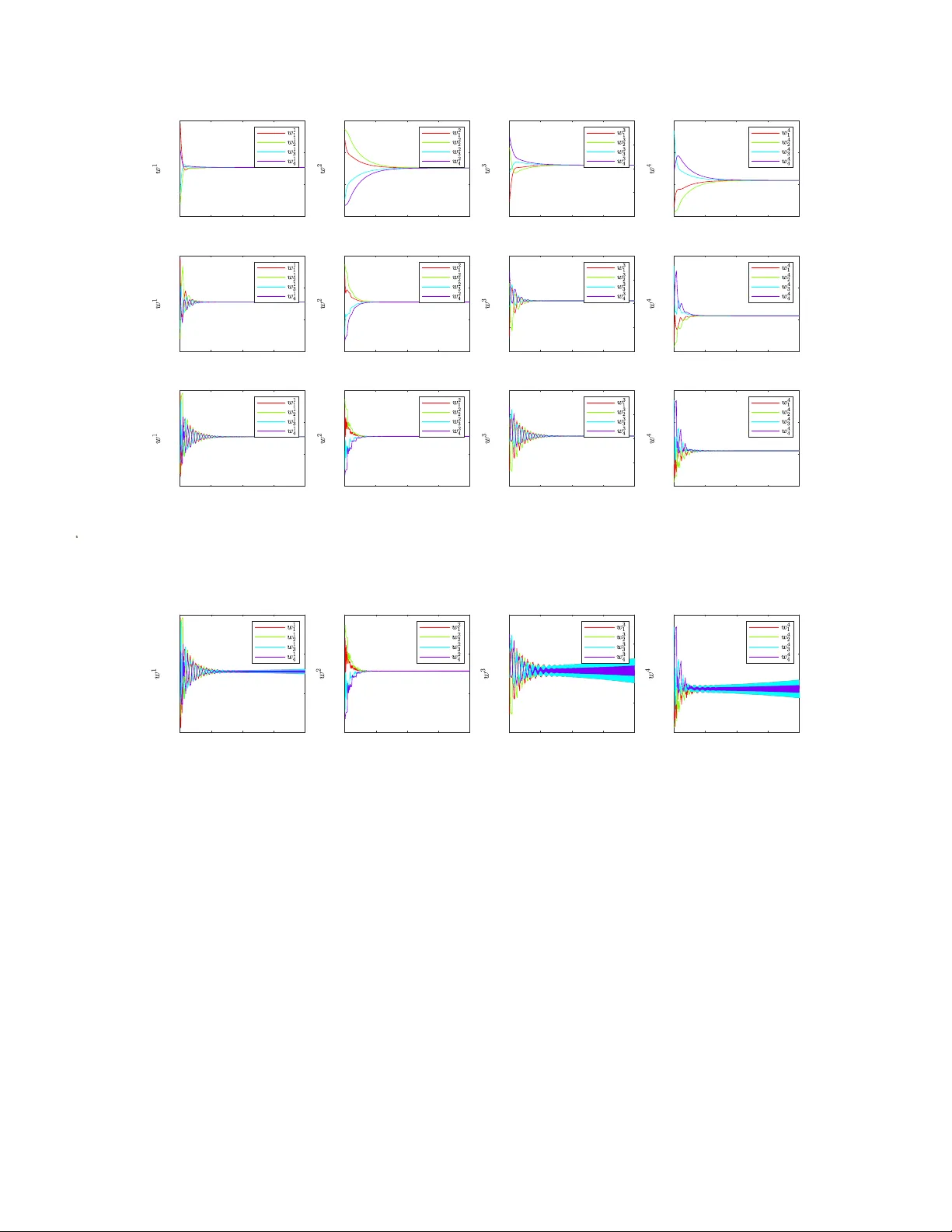
1 Consensus in Multi-Agent Systems with Uniform and Nonuniform Communication Delays Shokoufeh Naderi, Maude J. Blondin, Member , IEEE , S ´ ebastien Roy Abstract —This paper analyzes consensus in multi-agent sys- tems under uniform and nonuniform communication delays, a key challenge in distributed coordination with applications to robotic swarms. It inv estigates the conver gence of a consensus algorithm accounting for delays across communication links in a connected, undirected graph. Novel con vergence results are derived using Rouch ´ e’ s theorem and L yapunov-based stability analysis. The system is shown to reach consensus at a steady- state value giv en by a weighted av erage determined by the delay distribution, with stability ensured under explicit parameter bounds. Both uniform and nonunif orm delay scenarios are analyzed, and the corresponding con vergence v alues are explicitly derived. The theor etical r esults ar e validated through simulations, which explore the impact of delay heterogeneity on consensus outcomes. Furthermore, the algorithm is implemented and ex- perimentally tested on a swarm of QBO T3 ground robots to solve the rendezvous problem, demonstrating the agents’ ability to con verge to a common location despite realistic communication constraints, thus confirming the algorithm’s robustness and practical applicability . The results provide guidelines for de- signing consensus pr otocols that tolerate communication delays, offer insights into the relationship between network delays and coordination performance, and demonstrate their applicability to distributed robotic systems. Index T erms —Multi-Agent Systems, Consensus Algorithms, Nonuniform Delays, Distrib uted Optimization, Robotic Swarms, Rendezvous Problem I . I N T R O D U C T I O N Multi-agent systems ha ve become a po werful approach for solving complex optimization and consensus problems in a distributed manner . In recent years, researchers have extended distributed optimization methods to handle multi- objectiv e problems, in which agents seek to optimize mul- tiple objectiv e functions simultaneously . One such example is the algorithm proposed by Blondin and Hale [1], which enables a network of agents to collaborati vely explore Pareto- optimal solutions by e xchanging information weighted by each agent’ s prioritization of others’ objectives. That algorithm was prov en to con verge under ideal, delay-free communication. In practical networks, howe ver , communication delays are unav oidable due to transmission and processing latencies. These delays can degrade or ev en prev ent the con vergence of distributed algorithms if not properly accounted for . This paper All authors are with the Department of Electrical Engineering and Computer Engineering, Uni versit ´ e de Sherbrooke, Sherbrooke, QC, Canada. Contacts for the authors: Shokoufeh.Naderi@USherbrooke.ca, Maude.Blondin2@USherbrooke.ca, Sebastien.Roy13@USherbrooke.ca. This work has been submitted to the IEEE for possible publication. Copyright may be transferred without notice, after which this version may no longer be accessible. extends the algorithm of Blondin and Hale by analyzing its con vergence properties under constant communication delays. T wo delay scenarios are considered: uniform delays, where all communication links hav e the same constant delay , and nonuniform delays, where different links may have dif ferent (but fixed) delays. The focus is on establishing rigorous con- ver gence guarantees under these delays and quantifying how delays af fect the algorithm’ s performance and final outcomes. The effect of communication delays on consensus and distributed optimization has been extensi vely studied in the control and multi-agent systems (MASs) literature. Early works showed that consensus (agreement to a common v alue) can still be achieved in the presence of bounded time de- lays, though under more restrictive conditions. For instance, Olfati-Saber and Murray sho wed in [2] that for continuous- time consensus, if the interaction topology remains connected ov er time, the agents can reach agreement despite uniform communication delays. Subsequent studies in discrete-time systems provided more quantitativ e conditions. Bliman and Ferrari-T recate [3] obtained exact delay bounds for av erage consensus on fixed networks, showing how large a single delay , or multiple constant delays, can be before consensus on the av erage of the initial states is lost. Similarly , W ang et al. derived an upper bound on delay tolerance for consensus of identical agents [4]. These works, howe ver , generally assumed a uniform delay on all communication links for analytical tractability . Researchers hav e gradually relaxed the uniform-delay as- sumption, recognizing that equal delays on all links are an unrealistic simplification. For instance, Reh ´ ak and L ynnyk [5] showed that for consensus of identical agents with heteroge- neous input delays, exact synchronization cannot, in general, be achieved; instead, a bounded steady-state disagreement remains. Similarly , Lin and Jia [6] analyzed second-order consensus protocols in discrete-time systems with nonuniform communication delays and dynamically changing topologies, deriving con ver gence conditions using properties of nonnega- tiv e matrices. The increased comple xity of nonuniform delays often ne- cessitates more advanced analytical tools, such as L yapunov methods or spectral analysis, to establish stability guarantees. T o analyze the conv ergence of the multi-objective algorithm under delays, this paper employs two complementary ana- lytical techniques: Rouch ´ e’ s theorem from complex analysis and L yapunov-based stability analysis. In the uniform-delay case, an application of Rouch ´ e’ s theorem to the multi-agent domain is presented. Rouch ´ e’ s theorem has been used in stability analysis of time-delay differential equations [7], but 2 to our knowledge, it has not been applied to prov e con ver- gence of distributed optimization or consensus algorithms. By expressing the algorithm’ s delayed-update dynamics as a characteristic equation in the complex domain, Rouch ´ e’ s theorem is used to show that all eigen values of the update mapping remain inside the unit circle under a certain step-size condition. This approach yields an exact stability condition for the uniform delay case. For the more general nonuniform-delay scenario, a L yapunov-based analysis is used. L yapunov stability theory is a common tool for handling time-varying delays in networked systems [2]. A L yapunov function is designed to account for the delayed information at each communication link, and a L yapunov-based linear matrix inequality (LMI) condition is used to show that the consensus error decays to zero. Another key contribution of this work is determining the exact non-average conv ergence value of the algorithm under delays. In classical average consensus algorithms without delays, all agents conv erge to the uniform average of their initial values [1], [3]. Under delays, prior work typically still prov es con ver gence to an average of the initial values [2], [8]– [12] due to the self-delays considered in their update rules. In reality , an agent has essentially zero delay in accessing its own state, while communication delays occur only on links between different agents. Removing this artificial self- delay—while more realistic—breaks the symmetry that pre- serves the uniform average, making the analysis significantly more challenging and typically resulting in con ver gence to a weighted (non-uniform) av erage. In contrast to prior studies that often retain self-delays, this work explicitly models zero self-delays. This modeling choice preserves con vergence while providing a more realistic delay model. The exact (weighted) con vergence v alue is then rigorously deriv ed for both uniform and nonuniform delay cases. For the uniform-delay case on a regular graph, an explicit and constructiv e upper bound on the step size is deri ved that guarantees con vergence. While many prior works on consensus and distributed optimization require the step size to be sufficiently small for stability , the resulting conditions are typically implicit — expressed in terms of the spectral radius of the iteration matrix [13], [14], the maximum eigen value of the Laplacian [15], [16], or Lipschitz constants of local objectiv es [17], [18] — and require eigen value computations or iterati ve verification. In contrast, our bound is closed- form, depends only on easily computable graph in variants (maximum and average degree) and the delay , and does not require solving eigen values, making it suitable for analysis and implementation in large-scale networks. Finally , all theoretical results are validated through simula- tions and physical experiments on a multi-robot testbed. The delayed-information consensus algorithm is implemented on a set of Quanser QBot3 mobile robots that communicate over W i-Fi with induced constant latency to solve the rendezvous problem. The experimental results confirm robustness to com- munication delays. The rest of the paper is or ganized as follo ws. Section II revie ws the multi-objective multi-agent optimization algorithm from [1] and introduces our delay models and problem formu- lation. Section III presents the conv ergence analysis for the uniform delay case using Rouch ´ e’ s theorem, the nonuniform delay case using a L yapunov-based analysis, and the deriv a- tion of explicit con vergence v alues and the step size bound. Section IV provides simulation and experimental results that validate the theoretical findings. Finally , Section V concludes the paper and outlines future directions. I I . P R E L I M I N A R I E S A N D P R O B L E M D E S C R I P T I O N Consider a MAS comprising n agents that interact ov er a connected, undirected graph G = ( V , E ) , where V = { 1 , . . . , n } represents the set of agents, and E ⊆ V × V denotes the set of communication links. An edge ( i, j ) ∈ E indicates that agents i and j are neighbors and can exchange information directly . The graph has no self-loops, i.e., ( i, i ) / ∈ E for all i ∈ V , though each agent has access to its own data. The adjacency matrix H ( G ) = [ h i j ] ∈ R n × n is defined with entries h i j = 1 if ( i, j ) ∈ E , and 0 otherwise. The degree of agent i , denoted deg( i ) , is the number of its neighbors, given by deg( i ) = P n j =1 h i j . The degree matrix ∆( G ) ∈ R n × n is diag- onal, with ∆ i i = deg ( i ) for i = 1 , . . . , n , and the maximum degree is ∆ max = max i ∈ [ n ] deg( i ) . The Laplacian matrix of the graph is defined as L ( G ) = ∆( G ) − H ( G ) , capturing the network’ s connectivity properties. For the remainder of this paper , the graph notation G is omitted, and the Laplacian, degree, and adjacency matrices are simply denoted as L , ∆ , and H , respecti vely . Throughout the paper , for a matrix M = [ m i j ] , the notation m i j (or [ M ] i j ) denotes the entry in the i -th row and j -th column of M . Each agent i maintains a priority vector w i ( k ) = [ w i 1 ( k ) , w i 2 ( k ) , . . . , w i n ( k )] ∈ R 1 × n at time step k , which ev olves according to the update rule w i ( k + 1) = w i ( k ) + c n X j =1 h i j ( w j ( k − τ ij ) − w i ( k )) (1) for k ≥ τ max , with initial conditions w i ( k ) = w i (0) ∈ R n for k = 0 , 1 , . . . , τ max − 1 . Here, τ max = max ( i,j ) ∈E τ ij is the maximum communication delay , and τ ij is the nonnegati ve integer delay from agent j to agent i , satisfying τ ij = τ j i (due to the undirected nature of the graph) and τ ii = 0 . The priority vectors are used to weigh local objective functions in a multi-objectiv e optimization (MOO) problem, formulated as min x ∈ A f ( x ) = n X i =1 w i f i ( x ) , (2) where f ( x ) is the global objective function, f i : R m → R is the local objecti ve function known only to agent i , and m is the number of decision variables. A ⊆ R m is the feasible region defined by the problem constraints, and x ∈ A represents a feasible solution. The weight w i = [ w i ] i reflects the priority of f i . The objecti ve is to achiev e consensus on the priority vectors, such that w i ( k ) → α ∈ R 1 × n for all i , enabling the agents to collaboratively solve the optimization problem (2) with agreed-upon weights. Ho wever , the presence of nonuniform communication delays τ ij , which vary across edges, poses 3 a significant challenge to the consensus process, as delayed information exchange disrupts coordination among agents. T raditional consensus algorithms often assume uniform delays or instantaneous communication, which limits their effecti ve- ness in practical scenarios like robotic swarms, where delays are heterogeneous due to network constraints. This paper addresses the problem of achie ving consensus in MASs under uniform and nonuniform delays, analyzing the con vergence properties and steady-state behavior of the system defined by (1), with practical validation through the rendezvous problem in a swarm of QBOT3 ground robots. I I I . M A I N R E S U LT S This section presents the core theoretical findings on the consensus behavior of the MAS described in the pre vious section, focusing on the effects of communication delays. The following theorems establish the exact consensus value and its properties. T o enhance clarity and simplify the analysis, the most basic case in volving a uniform delay of τ = d on a regular graph is first presented in Theorem 1. This result is then extended to handle nonuniform delays in Theorem 2. Prior to stating the theorems, Lemma 1 and Lemma 2 pro- vide foundational results that are essential for the subsequent proofs. Lemma 1. Consider the MAS described in the pr evious section, where each agent i updates its priority vector w i ( k ) accor ding to (1) . Define the network state matrix W ( k ) = [ w 1 ( k ); w 2 ( k ); . . . ; w n ( k )] ∈ R n × n . Then, the update rule in matrix form is W ( k + 1) = ( I − c ∆) W ( k ) + c τ max X m =1 H m W ( k − m ) , (3) wher e I is the n × n identity matrix, and H m = [ h i j · 1 { τ ij = m } ] is the adjacency matrix for edges with delay m , for m = 1 , . . . , τ max , with 1 { τ ij = m } = 1 if τ ij = m , and 0 otherwise. Pr oof. T o deri ve the matrix form of the update rule, the agent-lev el dynamics are transformed into a network-le vel representation, utilizing the adjacenc y structure defined by H m and the degree matrix ∆ . Begin with the agent-lev el update rule defined in (1). Since w i ( k ) is independent of j , the second term inside the summation, − c P n j =1 h i j w i ( k ) , simplifies to n X j =1 h i j w i ( k ) = w i ( k ) n X j =1 h i j = deg( i ) w i ( k ) , (4) where deg( i ) = P n j =1 h i j is the degree of node i , quantifying the number of neighbors. h i j = 1 if ( i, j ) ∈ E and 0 otherwise (noting that h i i = 0 ). In matrix form, this term across all agents becomes − c ∆ W ( k ) , where ∆ is the diagonal matrix with ∆ i i = deg( i ) , and the i -th row of ∆ W ( k ) is deg ( i ) w i ( k ) . Now , consider the delayed term c P n j =1 h i j w j ( k − τ ij ) , which aggregates contributions from neighbors with v arying delays τ ij . Since τ ij ranges from 1 to τ max , this sum is partitioned by delay values. For each delay m from 1 to τ max , the contrib ution from neighbors with τ ij = m is c P j : τ ij = m h i j w j ( k − m ) 1 . The total delayed influence is thus c n X j =1 h i j w j ( k − τ ij ) = c τ max X m =1 X j : τ ij = m h i j w j ( k − m ) . (6) This double summation groups the neighbor contributions by their respective delay lags. In matrix notation, the inner sum P j : τ ij = m h i j w j ( k − m ) corresponds to the i -th row of H m W ( k − m ) , where H m = [ h i j · 1 { τ ij = m } ] is the adjacency matrix isolating edges with delay m , and 1 { τ ij = m } is an indi- cator function ensuring only the appropriate j contribute. The outer sum over m from 1 to τ max aggregates all delayed terms, yielding c P τ max m =1 H m W ( k − m ) , where each H m W ( k − m ) represents the influence from neighbors at lag m , weighted by the network structure at that delay . Combining these terms, the agent-lev el update becomes w i ( k + 1) = w i ( k ) + c τ max X m =1 [ H m W ( k − m )] i − c [∆ W ( k )] i . (7) Aggregating across all agents, the netw ork state matrix W ( k ) = [ w 1 ( k ); w 2 ( k ); . . . ; w n ( k )] , where W ( k ) i j = [ w i ( k )] j is the j -th component of agent i ’ s priority vector , ev olves according to W ( k + 1) = W ( k ) + c τ max X m =1 H m W ( k − m ) − c ∆ W ( k ) . (8) This can be equiv alently expressed as W ( k + 1) = ( I − c ∆) W ( k ) + c τ max X m =1 H m W ( k − m ) . (9) Lemma 2. F or the system described in (3) , define the aug- mented state vector z i ( k ) ∈ R n ( τ max +1) × 1 as z i ( k ) = [ w i ( k ) T , w i ( k − 1) T , . . . , w i ( k − τ max ) T ] T . The system dynamics ar e governed by z i ( k + 1) = Az i ( k ) , wher e the state transition matrix A ∈ R n ( τ max +1) × n ( τ max +1) is A =        I − c ∆ cH 1 cH 2 · · · cH τ max I 0 0 · · · 0 0 I 0 · · · 0 . . . . . . . . . . . . . . . 0 0 · · · I 0        , wher e H = P τ max l =1 H l the adjacency matrix, and H l the adjacency matrix for edges with delay l (i.e ., ( H l ) i j = 1 if 1 P j : τ ij = m h i j w j ( k − m ) includes only those neighbors j of i where the delay τ ij = m . For example, cH 1 W ( k − 1) represents the influence from neighbors with delay τ ij = 1 . The i -th row of H 1 W ( k − 1) is [ H 1 W ( k − 1)] i = n X j =1 [ H 1 ] i j w j ( k − 1) = X j : τ ij =1 h i j w j ( k − 1) . (5) This is the weighted sum of the previous state w j ( k − 1) for all j connected to i with a delay of 1. 4 τ ij = l , and 0 otherwise). Define the vector V ∈ R n ( τ max +1) as V = " β 1 T , β c 1 T τ max X l =1 H l , β c 1 T τ max X l =2 H l , . . . , β c 1 T H τ max # T , (10) wher e β  = 0 is a scalar , and 1 = [1 , . . . , 1] T ∈ R n is the column vector of ones. In the rest of the paper , as is the case her e, 1 denotes a column vector of ones with dimension n unless otherwise specified. Then, V is a left eigen vector of A with eigen value 1 (i.e., V T A = V T ), and the quantity V T z i ( k ) = β 1 T w i ( k ) + β c τ max X m =1 1 T τ max X l = m H l ! w i ( k − m ) is conserved, implying that V T z i ( k ) = V T z i (0) for all k ≥ 0 . Pr oof. T o establish conservation, it is first verified that V is a left eigenv ector of A with eigen value 1. This means V T A = V T , implying that applying A to z i ( k ) does not change the projection along V T . Expressing V T in block form, where each block is a row vector in R 1 × n , giv es V T = " β 1 T , β c 1 T τ max X l =1 H l , β c 1 T τ max X l =2 H l , . . . , β c 1 T H τ max # . The matrix A has τ max + 1 block rows and columns, where each block is of size n × n . W e can then determine V T A by multiplying each block of V T by the corresponding column blocks of A , as follows: V T A = [ β 1 T , β c 1 T τ max X l =1 H l , . . . , β c 1 T τ max X l = τ max − 1 H l , β c 1 T H τ max ]        I − c ∆ cH 1 cH 2 · · · cH τ max I 0 0 · · · 0 0 I 0 · · · 0 . . . . . . . . . . . . . . . 0 0 · · · I 0        . • First component (block 1) : This corresponds to the first block column of A , [ I − c ∆ , I , 0 , . . . , 0] T : β 1 T ( I − c ∆) + β c 1 T τ max X l =1 H l ! I = β 1 T − β c 1 T ∆ + β c 1 T τ max X l =1 H l . Since H = P τ max l =1 H l (the de gree matrix counts all edges incident to each node, aggregated across all delays), we hav e 1 T ∆ = 1 T H = 1 T P τ max l =1 H l . Thus, − β c 1 T ∆ + β c 1 T P τ max l =1 H l = 0 . So, the first component is β 1 T , matching the first block of V T . • Second component (block 2) : This corresponds to the second block column of A , [ cH 1 , 0 , I , 0 , . . . , 0] T : β 1 T ( cH 1 ) + β c 1 T τ max X l =2 H l ! I = β c 1 T H 1 + τ max X l =2 H l ! = β c 1 T τ max X l =1 H l , which matches the second block of V T . • Third component (block 3) : This corresponds to the third block column, [ cH 2 , 0 , 0 , I , 0 , . . . , 0] T : β 1 T ( cH 2 ) + β c 1 T τ max X l =3 H l ! I = β c 1 T H 2 + β c 1 T τ max X l =3 H l = β c 1 T H 2 + τ max X l =3 H l ! = β c 1 T τ max X l =2 H l , matching the third block of V T . • General m -th component ( m = 2 , . . . , τ max ) : The m -th block column of A has cH m − 1 in the first block, I in the ( m − 1) -th block (if m − 1 ≥ 2 ), and zeros elsewhere: β 1 T ( cH m − 1 ) + β c 1 T τ max X l = m H l ! I = β c 1 T H m − 1 + β c 1 T τ max X l = m H l = β c 1 T τ max X l = m − 1 H l , which matches the m -th block of V T . • Final component (block τ max + 1 ) : The last block column of A is [ cH τ max , 0 , . . . , 0] T , so β 1 T ( cH τ max ) + 0 + · · · + 0 = β c 1 T H τ max , matching the last block of V T . Thus, V T A = V T , confirming that V is a left eigen vector of A with eigen value 1. Giv en the system dynamics z i ( k + 1) = Az i ( k ) , apply V T to both sides V T z i ( k + 1) = V T ( Az i ( k )) = ( V T A ) z i ( k ) . Since V T A = V T , this becomes V T z i ( k + 1) = V T z i ( k ) . This recurrence holds for all k . Starting at k = 0 , we hav e V T z i (1) = V T z i (0) , V T z i (2) = V T z i (1) = V T z i (0) , . . . , so by induction, V T z i ( k ) = V T z i (0) for all k ≥ 0 . The quantity V T z i ( k ) is therefore conserved. The conserved quantity is V T z i ( k ) = β 1 T w i ( k ) + β c 1 T τ max X l =1 H l ! w i ( k − 1) + β c 1 T τ max X l =2 H l ! w i ( k − 2) + · · · + β c  1 T H τ max  w i ( k − τ max ) , which can be written as V T z i ( k ) = β 1 T w i ( k ) + β c τ max X m =1 1 T τ max X l = m H l ! w i ( k − m ) . This expression weighs the current state and delayed states by factors that depend on the graph structure and delays, reflecting 5 the influence of delayed interactions in the consensus process. In the next two subsections, the con ver gence proofs and con- sensus v alues for MASs with uniform delays and non-uniform delays are presented. The uniform delay proof (Lemma 3) assumes a regular graph, where all agents have the same degree, enabling spectral analysis via Rouch ´ e’ s theorem to deriv e a precise step size condition for stability . This assump- tion simplifies the eigen value analysis by ensuring the degree matrix ∆ commutes with the Laplacian’ s eigen vectors, making V T ∆ V diagonal, which is particularly applicable to structured networks such as rings or grids. The non-uniform delay proof (Lemma 4) applies to general graph topologies without requiring regularity and employs L yapunov theory to establish asymptotic stability . While this approach cov ers uniform delays as a special case, it does not use the structural properties of regular graphs to provide an explicit step size condition. Presenting both proofs offers complementary insights: the uniform-delay proof pro vides a precise design parameter for regular graphs, while the non- uniform-delay proof ensures robustness for arbitrary graphs and heterogeneous delays, addressing a broader range of practical scenarios in distributed systems. A. Uniform delays Lemma 3. Consider the MAS in Lemma 1 with a uniform delay τ ij = d for all ( i, j ) ∈ E and k ≥ 1 . The system evolves accor ding to the dynamics W ( k + 1) = ( I − c ∆) W ( k ) + cH W ( k − d ) , (11) wher e w i ( k ) = w i (0) for k = − d + 1 , . . . , − 1 , 0 , and δ 1 = 1 n P n k =1 deg( k ) is the avera ge degr ee of the graph. If 0 < c < min  1 dδ 1 , 2 ∆ max  , then the system con verges to a consensus, i.e., for each component j = 1 , . . . , n and some α j ∈ R , w j ( k ) → α j 1 as k → ∞ . Here , w j ( k ) = [ w 1 j ( k ) , w 2 j ( k ) , . . . , w n j ( k )] T ∈ R n denotes the j -th column of the state matrix W ( k ) , so w j ( k ) → α j 1 means that, as k → ∞ , all agents shar e the same value α j for the j -th objective (i.e., w 1 j ( k ) = w 2 j ( k ) = · · · = w n j ( k ) = α j ). Pr oof. See Appendix I. 1) Effect of step size c and comparison of stability bounds: The step size c in the consensus algorithm update rule, giv en by (1) plays a critical role in balancing con ver gence speed and stability . The term P n j =1 h i j ( w j ( k − τ ij ) − w i ( k )) in (1) computes a weighted sum of dif ferences between node i ’ s current state w i ( k ) and the delayed states of its neighbors w j ( k − τ ij ) , where h i j represents the connection weight from node j to node i . This sum acts as a correcti ve signal: if w i ( k ) is less than its neighbors’ delayed states, the sum is positiv e, increasing w i ( k + 1) ; if greater , the sum is negativ e, decreasing w i ( k + 1) . The step size c directly scales this correctiv e signal, determining the magnitude of the adjustment applied to w i ( k ) . A larger c , makes the update bigger , pushing the node’ s state more aggressiv ely toward its neighbors, while a smaller c makes the update smaller , adjusting the node’ s state more gradually . Howe ver , because the updates rely on delayed information, a large c might cause nodes to overshoot their targets. For example, if two nodes are adjusting based on each other’ s past states, they could overcorrect and oscillate instead of settling down. In extreme cases, this could prevent con vergence altogether . Thus, c controls how aggressi vely node i responds to discrepancies with its neighbors, balancing the trade-of f between rapid alignment and the risk of instability introduced by relying on delayed information. A larger bound on c accelerates con vergence, thereby de- creasing the number of steps required to reach consensus. Con versely , a smaller c limits the adjustment per step, which comes at the cost of slower con vergence, necessitating more iterations. The seminal work by [9] introduced a bound on c using the Gershgorin Circle Theorem, yielding c < 1 ∆ max , which is more conservati ve than the Rouch ´ e bound. Adopting the Rouch ´ e bound thus allows for larger step sizes, optimizing con vergence speed while still guaranteeing stability , offering a practical advantage over the one found through the Gershgorin Circle Theorem, especially in systems where rapid consensus is prioritized. Theorem 1. Consider the MAS in Lemma 3, wher e the system con verg es to a consensus value α j . The consensus value is given by α j = P n i =1 (1 + cd deg( i )) w i j (0) n + 2 cd | E | , (12) wher e | E | is the number of edges in G . This is a weighted averag e of the initial conditions with weights 1+ cd deg( i ) n +2 cd | E | , that sum to 1. Then, α j  = 1 n P n i =1 w i j (0) (the uniform avera ge) unless G is r e gular (all de gr ees equal), and the consensus value satisfies min i w i j (0) ≤ α j ≤ max i w i j (0) . Pr oof. The proof is performed by modeling the delayed sys- tem in an augmented state space, using the dynamics from Lemma 1. The system’ s update rule, with uniform delay τ ij = d for all ( i, j ) ∈ E , is W ( k + 1) = ( I − c ∆) W ( k ) + cH W ( k − d ) . At con vergence to consensus, w i j ( k ) → α j for all i and each j , implying w i ( k ) → α T = [ α 1 , . . . , α n ] , and thus W ( k ) → W ∗ = 1 α T , where W ∗ = [ α T ; α T ; . . . ; α T ] has all rows equal to α T . At steady state, W ( k − d ) → W ∗ , so W ∗ = ( I − c ∆) W ∗ + cH W ∗ . (13) Substituting W ∗ = 1 α T into (13) and rearranging terms, we get ( I − c ∆) W ∗ = 1 α T − c ∆ 1 α T , H W ∗ = H 1 α T , where ∆ 1 = [deg(1) , deg (2) , . . . , deg( n )] T and H 1 = ∆ 1 (since [ H 1 ] i = P n j =1 h i j = deg( i ) for an undirected graph). Thus W ∗ = 1 α T − c ∆ 1 α T + cH 1 α T = 1 α T , confirming the steady-state condition. T o find α j , define the augmented state z i ( k ) = [ w i ( k ) , w i ( k − 1) , . . . , w i ( k − d )] T ∈ R ( d +1) n for agent i , that 6 stacks the current and previous priority vectors as columns, with dynamics z i ( k + 1) =      ( I − c ∆) w i ( k ) + cH w i ( k − d ) w i ( k ) . . . w i ( k − d + 1)      = Az i ( k ) , A =         I − c ∆ 0 · · · 0 cH I 0 · · · 0 0 0 I . . . . . . . . . . . . . . . . . . 0 0 0 0 · · · I 0         , (14) where A is ( d + 1) n × ( d + 1) n . At consensus, z i ( k ) → [ α, α, . . . , α ] T (length d + 1 ), and A [ α, α , . . . , α ] T = [ α, α, . . . , α ] T , since ( I − c ∆) α + cH α = α . From Lemma 2, the left eigen vector for the non-uniform delay case is expressed as in (10), satisfying V T A = V T . For uniform delay τ ij = d , all edges have delay d , so τ max = d , and H l = 0 for l  = d , H d = H . Thus, the sums simplify to 1 T P τ max l = k H l = 1 T H = [deg (1) , . . . , deg( n )] for k ≤ d , and 0 otherwise. The eigen vector becomes V T = [ β 1 T , cβ [deg (1) , . . . , deg ( n )] , . . . , cβ [deg (1) , . . . , deg ( n )]] , with d copies of cβ [deg(1) , . . . , deg ( n )] . The lemma estab- lishes that V T z i ( k ) = V T z i (0) for all k ≥ 0 . This conserved quantity is computed to find α j . Compute V T z i ( k ) as follows: V T z i ( k ) = β 1 T w i ( k )+ cβ d X m =1 [deg(1) , . . . , deg ( n )] w i ( k − m ) . At consensus, w i ( k − m ) → α , and V T [ α, α, . . . , α ] T = β 1 T α + cβ d X m =1 [deg(1) , . . . , deg ( n )] α = β nα j + cβ dα j n X i =1 deg( i ) = β α j ( n + 2 cd | E | ) , (15) using the handshaking lemma P n i =1 deg( i ) = 2 | E | . Initially , w i ( − m ) = w i (0) for m = 1 , . . . , d and we have V T z i (0) = β 1 T w i (0) + cβ d X m =1 [deg(1) , . . . , deg ( n )] w i (0) = β n X j =1 w i j (0) + cβ d n X i =1 deg( i ) w i j (0) . (16) From (15) and (16), we hav e: β α j ( n + 2 cd | E | ) = β n X i =1 (1 + cd deg( i )) w i j (0) , α j = P n i =1 (1 + cd deg( i )) w i j (0) n + 2 cd | E | , thus proving (12). The weights are 1+ cd deg( i ) n +2 cd | E | , which are positiv e since c > 0 , deg( i ) ≥ 1 (as G is connected), and n + c · 2 | E | > 0 (with | E | ≥ n − 1 ). Their sum is: P n i =1 (1 + cd deg( i )) n + 2 cd | E | = n + cd · 2 | E | n + 2 cd | E | = 1 . For α j  = 1 n P n i =1 w i j (0) , compute α j − 1 n n X i =1 w i j (0) = P n i =1 (1 + cd deg( i )) w i j (0) n + 2 cd | E | − P n i =1 w i j (0) n = 1 n ( n + 2 cd | E | ) n n X i =1 (1 + cd deg( i )) w i j (0) − ( n + 2 cd | E | ) n X i =1 w i j (0) ! = cd n + 2 cd | E | n X i =1 deg( i ) w i j (0) − 2 | E | n n X i =1 w i j (0) ! , where 2 | E | n = ¯ d (mean degree). This is zero if n X i =1 deg( i ) w i j (0) = ¯ d n X i =1 w i j (0) , which holds when deg( i ) = ¯ d for all i (regular graph), otherwise it is non-zero due to degree variation. For the last part of the theorem, since 1+ cd deg( i ) n +2 cd | E | > 0 and P n i =1 1+ cd deg( i ) n +2 cd | E | = 1 , α j is a con ve x combination 2 . Let m j = min i w i j (0) and M j = max i w i j (0) . Then α j ≥ n X i =1 1 + cd deg( i ) n + 2 cd | E | m j = m j , α j ≤ n X i =1 1 + cd deg( i ) n + 2 cd | E | M j = M j , thus m j ≤ α j ≤ M j , completing the proof. B. Nonuniform delays Building on the uniform delay case, the next lemma and theorem extend the analysis to the general scenario of nonuni- form delays, where τ ij varies across edges, addressing the challenges posed by heterogeneous communication lags in practical networks. Lemma 4 (L yapunov Stability with LMI) . Consider the MAS in Lemma 1. The dynamics ar e w j ( k + 1) = ( I − c ∆) w j ( k ) + c τ max X m =1 H m w j ( k − m ) , wher e L 1 = 0 . The augmented state z ( k ) ∈ R n ( τ max +1) is z ( k ) = [ w j ( k ) T , w j ( k − 1) T , . . . , w j ( k − τ max ) T ] T , with dynamics z ( k + 1) = Az ( k ) , 2 A con vex combination is a linear combination of points where all coefficients are non-negati ve and add up to 1 [19]. 7 A =        I − c ∆ cH 1 cH 2 · · · cH τ max I 0 0 · · · 0 0 I 0 · · · 0 . . . . . . . . . . . . . . . 0 0 · · · I 0        . (17) The system conver ges to consensus, i.e., w i j ( k ) → α j for all i as k → ∞ and for some α j ∈ R , if ther e exists a positive definite matrix P ∈ R n ( τ max +1) × n ( τ max +1) satisfying the LMI A T QP QA − QP Q < 0 , wher e Q ∈ R n ( τ max +1) × n ( τ max +1) , defined as Q = I − 1 n ( τ max + 1) 1 n ( τ max +1) 1 T n ( τ max +1) , pr ojects onto the subspace orthogonal to the consensus dir ec- tion. A candidate P is given by P = τ max X d =0 C d ( L + δ I n ) C T d with δ > 0 small to ensur e P is positive definite and C d = [0 , . . . , I , . . . , 0] with I in the ( d + 1) -th bloc k and zer os elsewher e. This LMI pr ovides a suf ficient condition for consensus con verg ence and serves as a numerical feasibility test for a given step size c . Although it does not yield an explicit analytical bound on c , it can be used to compute the lar gest admissible c numerically . Pr oof. See Appendix II. Theorem 2. Consider the MAS in Lemma 4, wher e the system con verg es to a consensus value α j . The consensus value is given by α j = P n i =1  1 + c P j ∈N i τ ij  w i (0) n + 2 c P ( i,j ) ∈ E τ ij , (18) wher e P j ∈N i τ ij is the total delay incoming to agent i , and P ( i,j ) ∈ E τ ij is the total delay over all edges (counting each edge once due to undirectedness). This is a weighted average of initial conditions with weights 1+ c P j ∈N i τ ij n + c P ( i,j ) ∈ E τ ij , which sum to 1. Then, α j  = 1 n P n j =1 w i j (0) (the uniform average) unless P j ∈N i τ ij is equal for all i , and the consensus value satisfies min i w i j (0) ≤ α j ≤ max i w i j (0) . Pr oof. At steady state, the system con ver ges to consensus, where W ( k ) → W ∗ = 1 α T , with α T = [ α 1 , . . . , α n ] repre- senting the consensus v alues across all agents and components. Substituting this into the update rule W ( k + 1) = ( I − c ∆) W ( k ) + c P τ max m =1 H m W ( k − m ) , and noting that at steady state all delayed states also equal W ∗ (since W ( k − m ) → W ∗ for all m ), one can obtain W ∗ = ( I − c ∆) W ∗ + c τ max X m =1 H m W ∗ . T o determine α , define the augmented state vector z i ( k ) = [ w i ( k ) T , w i ( k − 1) T , . . . , w i ( k − τ max ) T ] T ∈ R n ( τ max +1) , which stacks the current and all delayed priority vectors for agent i . The dynamics are governed by z i ( k + 1) = Az i ( k ) , (19) where the state transition matrix A is as in (17). From Lemma 2, the vector V in (10) is a left eigenv ector of A with eigen value 1, satisfying V T A = V T . The lemma also establishes that the quantity V T z i ( k ) is conserved, i.e., V T z i ( k ) = V T z i (0) for all k ≥ 0 . This conserved quantity is computed to find the consensus value α j . The expression for V T z i ( k ) from the lemma is V T z i ( k ) = β 1 T w i ( k ) + β c τ max X m =1 1 T τ max X l = m H l ! w i ( k − m ) . (20) At consensus, w i ( k ) → α j 1 for all i and all delayed states w i ( k − m ) → α j 1 (since the system has conv erged and delays are finite). Substituting this into (20), we hav e V T z i ( k ) → β 1 T ( α j 1 ) + β c τ max X m =1 1 T τ max X l = m H l ! ( α j 1 ) . Since 1 T 1 = n , the first term is β 1 T ( α j 1 ) = β nα j . The sum in the abov e can be rewritten as τ max X m =1 1 T τ max X l = m H l ! 1 = τ max X m =1 τ max X l = m 1 T H l 1 . Since 1 T H l 1 = P n i =1 P n j =1 ( H l ) i j = 2 P ( i,j ) ∈ E : τ ij = l 1 (each edge with delay l is counted twice in an undirected graph), the summation can be reordered as follows: 3 : τ max X m =1 τ max X l = m 1 T H l 1 = τ max X l =1 l · 1 T H l 1 = 2 τ max X l =1 l X ( i,j ) ∈ E : τ ij = l 1 = 2 X ( i,j ) ∈ E τ ij . The equality P τ max l =1 l P ( i,j ) ∈ E : τ ij = l 1 = P ( i,j ) ∈ E τ ij holds because the left-hand side computes the total delay across all edges. For each delay l , P ( i,j ) ∈ E : τ ij = l 1 counts edges with τ ij = l , and multiplying by l gives their delay contrib ution. Summing over l from 1 to τ max , each edge ( i, j ) contributes its delay τ ij exactly once, so P τ max l =1 l P ( i,j ) ∈ E : τ ij = l 1 = P ( i,j ) ∈ E τ ij . Thus, P τ max m =1  1 T P τ max l = m H l  1 = 2 P ( i,j ) ∈ E τ ij , and V T z i ( k ) → β nα j + 2 β cα j X ( i,j ) ∈ E τ ij . (21) 3 The equality P τ max m =1 P τ max l = m 1 T H l 1 = P τ max l =1 l · 1 T H l 1 holds as follows: • The left-hand side sums 1 T H l 1 over l from m to τ max for each m from 1 to τ max , counting 1 T H 1 1 once, 1 T H 2 1 twice, ..., 1 T H τ max 1 τ max times. • The right-hand side sums l · 1 T H l 1 over l from 1 to τ max , where l weighs the edge count by the delay , matching the left-hand side’s counting. Thus, both sides are equal due to the reordering of the summation according to the alignment of the delay contributions. 8 Initially , assuming w i ( − m ) = w i (0) for m = 1 , . . . , τ max , we hav e V T z i (0) = β 1 T w i (0) + β c τ max X m =1 1 T τ max X l = m H l ! w i (0) . Since w i (0) is the same for each m under this assumption, we hav e τ max X m =1 1 T τ max X l = m H l ! w i (0) = τ max X m =1 τ max X l = m 1 T H l !! w i (0) . The first term is β 1 T w i (0) = β P n i =1 w i (0) . Define ψ ( i ) = P j ∈N i τ ij . Then, τ max X m =1 1 T τ max X l = m H l = [ ψ (1) , . . . , ψ ( n )] , and V T z i (0) = β n X i =1 w i (0) + β c n X i =1 ψ ( i ) w i (0) . (22) Equating (21) and (22) and solving yields β n X i =1 w i (0) + β c n X i =1 ψ ( i ) w i (0) = nβ α j + 2 β cα j X ( i,j ) ∈ E τ ij . Since β  = 0 , both sides can be divided by β , leading to α j = P n i =1 (1 + cψ ( i )) w i (0) n + 2 c P ( i,j ) ∈ E τ ij . I V . S I M U L A T I O N S A N D E X P E R I M E N T S A. Simulations Before conducting real-world experiments, the proposed consensus algorithm is ev aluated through numerical simula- tions. The kinematic model of the QBot3 robot, along with the rele vant motion dynamics, terminology used on the QBot3 platform, and the control structure, are detailed in [20]. Each simulated agent follo ws the same update rule as described in Section III, interacting ov er a predefined commu- nication graph that includes nonuniform constant delays. These simulations allow us to verify the theoretical con ver gence guarantees in a controlled en vironment, visualize the dynamic behavior of the agents, and inv estigate the influence of delay parameters and step size on conv ergence speed and final values. For the simulation parameters and initial conditions, the same values as reported in [20] are adopted. The communica- tion delays between agents are modeled by the delay matrix τ =     0 7 1 5 7 0 5 5 1 5 0 6 5 5 6 0     . Figure 1 illustrates the time ev olution of the priority matrix columns for 4 agents over 4 seconds under three different step sizes. Each subplot sho ws the evolution of one column of W , with the curves corresponding to the values held by T ABLE I C O N V E R G E N C E T I M E A N D FI NA L C O N S E N S U S V A L U E S F O R D I FF E R E N T S T E P S I Z E S c ( 4 A G E N T S , N O N U N I F O R M D E L A Y S ) . c Con vergence time (s) α 1 α 2 α 3 α 4 0.05 3.65 0.2537 0.3046 0.2151 0.2266 0.15 1.78 0.2545 0.3083 0.2127 0.2245 0.25 1.43 0.2548 0.3102 0.2114 0.2235 0.35 1.82 0.2551 0.3113 0.2107 0.2229 0.45 2.26 0.2552 0.3120 0.2103 0.2225 0.55 2.69 0.2553 0.3125 0.2099 0.2223 the four agents. As observed in the simulations and consistent with the analysis, the step size c exhibits a non-monotonic effect on conv ergence speed. A small step size ( c = 0 . 05 ) yields smooth, monotonic con vergence b ut requires a long settling time. An intermediate value ( c = 0 . 25 ) provides the fastest conv ergence with only mild oscillations. A larger step size ( c = 0 . 55 ) significantly increases oscillatory behavior due to ov ercorrection based on delayed neighbor information, resulting in a long overall settling time despite faster initial correction. T able I reports the con ver gence times for the different step sizes. Con vergence time is defined as the first time instant when the maximum dif ference within each column falls below 10 − 4 and remains below thereafter . The values in the table show that an intermediate step size ( c = 0 . 25 ) yields the fastest con vergence, while o verly small or large v alues result in longer settling times due to slow adaptation or oscillatory behavior , respectiv ely . T o further validate the observed con vergence behavior , a reduced form of the LMI from Lemma 4 was numerically solved. By projecting the dynamics onto the disagreement sub- space (i.e., removing the consensus mode), numerical issues associated with the marginal eigen value at 1 were av oided, and a discrete-time L yapunov LMI was solved on the resulting reduced system. A bisection search ov er the step size c was performed to determine the lar gest value ensuring feasibility of the strict LMI on the reduced system. This yielded a maximum admissible step size of c max = 0 . 58 . This bound is consistent with the simulation results and provides a quantitati ve stability reference for the step-size selection reported in T able I. Fig- ure 2 illustrates the system beha vior for a step size slightly abov e this bound. When c = 0 . 59 , the trajectories no longer con verge to consensus and instead exhibit growing oscillations, indicating div ergence of the disagreement dynamics. This observation agrees with the LMI-based analysis and confirms that step sizes exceeding the admissible limit lead to loss of con vergence. B. Experiments T o validate the theoretical conv ergence results in a real- world setting, the proposed consensus algorithm is imple- mented on a swarm of four Quanser QBot3 mobile ground robots. Each QBot3 is equipped with onboard computing, differential-dri ve motors, and wireless communication capa- bilities, enabling decentralized interaction in physical en viron- ments. 9 0 1 2 3 4 Time 0.1 0.2 0.3 0.4 0 1 2 3 4 Time 0 0.2 0.4 0.6 0 1 2 3 4 Time 0 0.1 0.2 0.3 0.4 0 1 2 3 4 Time 0 0.2 0.4 0.6 0 1 2 3 4 Time 0.1 0.2 0.3 0.4 0 1 2 3 4 Time 0 0.2 0.4 0.6 0 1 2 3 4 Time 0 0.1 0.2 0.3 0.4 0 1 2 3 4 Time 0 0.2 0.4 0.6 0 1 2 3 4 Time 0.1 0.2 0.3 0.4 0 1 2 3 4 Time 0 0.2 0.4 0.6 0 1 2 3 4 Time 0 0.1 0.2 0.3 0.4 0 1 2 3 4 Time 0 0.2 0.4 0.6 Fig. 1. Time ev olution of the priority matrix columns for 4 agents ov er 4 seconds. Each row corresponds to a different step size c : c = 0 . 05 (first row), c = 0 . 25 (second row), and c = 0 . 55 (third ro w). 0 1 2 3 4 Time 0.1 0.2 0.3 0.4 0 1 2 3 4 Time 0 0.2 0.4 0.6 0 1 2 3 4 Time 0 0.1 0.2 0.3 0.4 0 1 2 3 4 Time 0 0.2 0.4 0.6 Fig. 2. Time evolution of the priority matrix columns for c = 0 . 59 , slightly abov e the LMI-certified bound c max = 0 . 58 . The algorithm was deployed using the QU ARC Simulink library , which interfaces with MA TLAB/Simulink to compile and run control code directly on the robots. Robot positions were tracked using a motion capture system composed of Op- tiT rack infrared cameras and Motiv e software, which provided estimates of each robot’ s position and orientation. These data were streamed into the Simulink environment for logging and ev aluation. In the experiments, each robot is dri ven by a simple tracking controller that con verts the consensus reference points generated by the algorithm into linear and angular velocity commands. The linear v elocity is determined from the distance to the reference using a bounded sigmoid mapping, while the angular velocity is generated by a proportional–deriv ativ e con- troller acting on the heading error . The consensus update law and the controller were implemented in MA TLAB/Simulink. At each simulation step, the consensus algorithm updated the rendezv ous reference points for each agent. The control signals were then generated and applied to the QBot3’ s inv erse kinematic model. While no artificial or predefined delays were introduced in the implementation, delays naturally arise in the physical system due to factors such as communication latency , asyn- chronous processing times, and Wi-Fi transmission variability . These real-time ef fects result in nonuniform delays across agents, e ven though the algorithm itself does not explicitly incorporate or measure them. The exact values of these delays are unknown during experiments, pre venting us from com- puting the theoretical con vergence value for direct compari- son. Nonetheless, experimental observations confirm that the agents’ priority vectors conv erge consistently , demonstrating the algorithm’ s robustness under practical communication con- ditions. Figure 3 illustrates the experimental time ev olution of the priority matrix columns for c = 0 . 20 . The agents start from 10 0 5 10 Time 0.1 0.2 0.3 0.4 0 5 10 Time 0.2 0.25 0.3 0.35 0.4 0.45 0 5 10 Time 0 0.1 0.2 0.3 0 5 10 Time 0.2 0.3 0.4 0.5 Fig. 3. Experimental time ev olution of the priority matrix columns for c = 0 . 20 . the randomly generated initial priority matrix W (0) =     0 . 1000 0 . 4189 0 . 0587 0 . 4224 0 . 3513 0 . 2000 0 . 0548 0 . 3939 0 . 2165 0 . 2407 0 . 3000 0 . 2427 0 . 2205 0 . 2451 0 . 0344 0 . 5000     . Despite these different initial values, all trajectories con verge to a common v alue, demonstrating consensus among the agents. The transient oscillations observed in the first seconds are consistent with the delayed update dynamics predicted by the analysis and gradually v anish as the system approaches the steady state. V . C O N C L U S I O N This paper analyzed the con vergence of a distributed multi- objectiv e optimization algorithm under constant communica- tion delays in MASs. For the uniform delay case, Rouch ´ e’ s theorem was used to derive exact stability conditions, while a L yapunov-based approach was employed for the nonuniform delay case. These analyses provide rigorous conv ergence guar- antees and explicit expressions for the consensus value and admissible step-size bounds. Simulation results and experi- ments on QBot3 robots validated the theoretical findings and demonstrated robustness to communication delays. Future work will consider extensions to time-v arying delays and fully asynchronous update schemes, in which agents operate on dif ferent clocks or update at dif ferent rates, beyond the communication-level asynchrony considered in this work. A P P E N D I X A P R OV I N G T H E C O N V E R G E N C E O F L E M M A 3 For each component j , the columns w j ( k ) = [ w 1 j ( k ) , . . . , w n j ( k )] T hav e the structure w j ( k + 1) = ( I − c ∆) w j ( k ) + cH w j ( k − d ) . Define the augmented state z j ( k ) = [ w j ( k ) T , w j ( k − 1) T , . . . , w j ( k − d ) T ] T ∈ R n ( d +1) , so the dynamics become z j ( k + 1) = Az j ( k ) , with A having the structure given in (14). Con vergence to consensus requires that the eigen value λ = 1 , corresponding to the consensus state, be on the unit circle ( | λ | = 1 ) and that all other eigen values of A be of magnitude less than 1 ( | λ | < 1 ). The characteristic polynomial is λ A I − A =        ( λ A − 1) I n + c ∆ 0 · · · 0 − cH − I λ A I n · · · 0 0 0 − I · · · 0 0 . . . . . . . . . . . . . . . 0 0 · · · − I λ A I n        . Using the block determinant formula for a matrix  A 11 A 12 A 21 A 22  , if A 22 is in vertible, det = det( A 22 ) det( A 11 − A 12 A − 1 22 A 21 ) . Here, A 11 = ( λ A − 1) I n + c ∆ ( n × n ), A 12 = [0 , · · · , 0 , − cH ] ( n × nd ), A 21 = [ − I , 0 , · · · , 0] T ( nd × n ), and A 22 =      λ A I n 0 · · · 0 − I λ A I n · · · 0 . . . . . . . . . . . . 0 · · · − I λ A I n      ( nd × nd ). The matrix A 22 is lo wer-triangular with λ A I n on the diagonal ( d times). Thus det( A 22 ) = det( λ A I n ) d = λ nd A . The in verse A − 1 22 (with n × n blocks) is upper-triangular: A − 1 22 =      λ − 1 A I n 0 · · · 0 λ − 2 A I n λ − 1 A I n · · · 0 . . . . . . . . . . . . λ − d A I n λ − d +1 A I n · · · λ − 1 A I n      , which is obtained by solving A 22 A − 1 22 = I . Then A − 1 22 A 21 = [ − λ − 1 A I n , − λ − 2 A I n , · · · , − λ − d A I n ] T , A 12 A − 1 22 A 21 = [0 , · · · , 0 , − cH ]      − λ − 1 A I n − λ − 2 A I n . . . − λ − d A I n      = cλ − d A H , A 11 − A 12 A − 1 22 A 21 = ( λ A − 1) I n + c ∆ − cλ − d A H . The determinant is det( λ A I − A ) = det( A 22 ) det( A 11 − A 12 A − 1 22 A 21 ) = λ nd A det  ( λ A − 1) I n + c ∆ − cλ − d A H  = det  λ d A ( λ A − 1) I n + cλ d A ∆ − cH  = det  λ d +1 A I n − λ d A ( I n − c ∆) − cH  . By substituting H = ∆ − L , define D ( λ A ) := ( λ d +1 A − λ d A ) I + c ( λ d A ∆ − ∆ + L ) . 11 The eigenv alues of L satisfy Lv i,L = λ i,L v i,L , where 0 = λ 1 ,L < λ 2 ,L ≤ · · · ≤ λ n,L ≤ 2∆ max . Moreo ver , since L is symmetric, it has an orthogonal eigen vector matrix V = [ v 1 ,L , . . . , v n,L ] , with V T V = I , meaning the eigenv ectors are orthonormal: each eigenv ector v i,L is normalized ( v T i,L v i,L = 1 , i.e., ∥ v i,L ∥ 2 = 1 ) and orthogonal to the others ( v T i,L v j,L = 0 for i  = j ). Specifically , for the first eigenv ector, v 1 ,L = 1 √ n 1 , which is the normalized form of 1 (since L 1 = 0 , and ∥ 1 ∥ 2 = √ n , so 1 √ n 1 has norm 1). For any matrix D , if V is orthogonal, det( V T D V ) = det( D ) . Thus, det( D ( λ A )) = det( V T D ( λ A ) V ) , and V T D ( λ A ) V =( λ d +1 A − λ d A ) I + c ( λ d A V T ∆ V − V T ∆ V + V T LV ) , where V T LV = diag ( λ 1 ,L , . . . , λ n,L ) and it is assumed that V T ∆ V = diag ( δ 1 , . . . , δ n ) , where δ i = v T i,L ∆ v i,L . This assumption states that the matrix V T ∆ V has no off-diagonal elements. This holds when the graph is regular , i.e., all nodes hav e the same degree deg i , so ∆ = deg i I and V T ∆ V = deg i I ; otherwise, V T ∆ V generally has non-zero off-diagonal elements, though these terms are smaller when the degrees are more uniform (e.g., when the variance in node degrees is low), making the approximation V T ∆ V ≈ diag ( δ 1 , . . . , δ n ) more accurate. The stability analysis focuses on the diagonal terms δ i , as the characteristic equation is ev aluated along each eigenspace of L , leading to a decoupled per-mode analysis. Thus V T D ( λ A ) V = diag  λ d +1 A − λ d A + c ( λ d A δ i − δ i + λ i,L )  n i =1 , det( D ( λ A )) = n Y i =1  λ d +1 A − (1 − cδ i ) λ d A − c ( δ i − λ i,L )  . The characteristic equation per each λ i,A is p i ( λ i,A ) = λ d +1 i,A − (1 − cδ i ) λ d i,A − c ( δ i − λ i,L ) = 0 . (23) For stability , roots must satisfy | λ i,A | < 1 except for the consensus mode. For i = 1 , λ 1 ,L = 0 , and it follows that p 1 ( λ 1 ,A ) = λ d +1 1 ,A − (1 − cδ 1 ) λ d 1 ,A − cδ 1 = 0 . Factoring p 1 ( λ 1 ,A ) using synthetic division yields p 1 ( λ 1 ,A ) = ( λ 1 ,A − 1)( λ d 1 ,A + cδ 1 λ d − 1 1 ,A + · · · + cδ 1 λ 1 ,A + cδ 1 ) . Letting q ( λ 1 ,A ) = λ d 1 ,A + cδ 1 ( λ d − 1 1 ,A + · · · + λ 1 ,A + 1) , and assuming a root | λ 1 ,A | ≥ 1 , we have λ d 1 ,A = − cδ 1 ( λ d − 1 1 ,A + · · · + λ 1 ,A + 1) , | λ 1 ,A | d ≤ cδ 1 d − 1 X k =0 | λ 1 ,A | k ≤ cδ 1 d | λ 1 ,A | d − 1 ≤ cδ 1 d. If c < 1 dδ 1 , then | λ 1 ,A | < 1 , contradicting | λ 1 ,A | ≥ 1 . Thus, all roots of q ( λ 1 ,A ) satisfy | λ 1 ,A | < 1 , so p 1 ( λ 1 ,A ) has one root at λ 1 ,A = 1 and d roots inside | λ 1 ,A | < 1 . Since Lv i,L = λ i v i,L , v T i,L (∆ − H ) v i,L = λ i,L = ⇒ δ i − h i = λ i,L . (24) Thus, For i > 1 , consider p i ( λ i,A ) = λ d +1 i,A − (1 − cδ i ) λ d i,A − ch i , where h i = δ i − λ i,L = v T i,L H v i,L > 0 . Rouch ´ e’ s theorem can be applied on the unit circle | λ A | = 1 to find the bound on c that ensures stability . Rouch ´ e’ s theorem states that if h ( λ i,A ) and g ( λ i,A ) are analytic inside and on | λ i,A | = 1 , and | g ( λ i,A ) | < | h ( λ i,A ) | on | λ i,A | = 1 , then p i ( λ i,A ) = h ( λ i,A ) + g ( λ i,A ) has the same number of roots inside | λ i,A | = 1 as h ( λ i,A ) . The goal is to choose h ( λ i,A ) with all d + 1 roots inside | λ i,A | = 1 , and ensure the magnitude of g ( λ i,A ) is strictly less than that of h ( λ i,A ) on the unit circle. Consider that p i ( λ i,A ) = h ( λ i,A ) + g ( λ i,A ) , where h ( λ i,A ) = λ d +1 i,A − (1 − cδ i ) λ d i,A , g ( λ i,A ) = − ch i . Roots of h ( λ i,A ) = λ d i,A ( λ i,A − (1 − cδ i )) are 0 ( d times) and 1 − cδ i , inside | λ i,A | = 1 if c < 2 δ i . On | λ i,A | = 1 , λ i,A = e iθ , and | h ( λ i,A ) | = | e idθ ( e iθ − (1 − cδ i )) | = | e iθ − (1 − cδ i ) | = q sin 2 θ + cos 2 θ + (1 − cδ i ) 2 − 2 cos θ (1 − cδ i ) = q 2 + c 2 δ 2 i − 2 cδ i − 2 cos θ (1 − cδ i ) = q (1 − cδ i )(2 − 2 cos θ ) + c 2 δ 2 i = p 2(1 − cos θ )(1 − cδ i ) + ( cδ i ) 2 , which ranges from cδ i (at cos θ = 1 ) to p 4(1 − cδ i ) + ( cδ i ) 2 (at cos θ = − 1 ). Meanwhile, | g ( λ i,A ) | = ch i . The minimum of | h ( λ i,A ) | is cδ i , and since δ i > h i = δ i − λ i,L for i > 1 (as λ i,L > 0 ), we have cδ i > ch i , ensuring | h ( λ i,A ) | > | g ( λ i,A ) | ev erywhere on the circle for i > 1 . Rouch ´ e’ s theorem applies if | g | < | h | on | λ i,A | = 1 , which is satisfied. Since h ( λ i,A ) has d + 1 roots inside | λ i,A | < 1 when c < 2 δ i , p i ( λ i,A ) has all d + 1 roots inside the unit circle. For i = 1 , the inequality fails ( δ 1 = v T 1 ,L H v 1 ,L ) since λ 1 ,L = 0 , but we do not apply Rouch ´ e’ s theorem here, as the roots of p 1 ( λ 1 ,A ) were computed directly (one root at λ 1 ,A = 1 and d roots inside | λ 1 ,A | < 1 ), and the consensus mode is handled separately to ensure λ 1 ,A = 1 is on the unit circle while cdδ 1 < 1 . T o find the bound on δ i , note that since V T V = I , we hav e P n j =1 ( v i,L ( j )) 2 = 1 , and since δ i = v T i,L ∆ v i,L = P n j =1 deg( j )( v i,L ( j )) 2 , we ha ve 0 ≤ δ i ≤ ∆ max , as deg( j ) ≤ ∆ max . Combining conditions, for i = 1 , c < 1 dδ 1 ensures one root at 1 and others inside the unit circle. For i > 1 , c < 2 δ i , and since δ i ≤ ∆ max , c < 2 ∆ max suffices. Thus, the system con verges to consensus if 0 < c < min  1 dδ 1 , 2 ∆ max  . A P P E N D I X B P R OV I N G T H E C O N V E R G E N C E O F L E M M A 4 Consider the following L yapunov-Krasovskii function for each component j : V j ( k ) = z ( k ) T QP Qz ( k ) , (25) with total L yapunov function gi ven by V ( k ) = P m j =1 V j ( k ) . The L yapunov stability conditions are verified analytically using the proposed L yapunov function. Specifically , it is shown that the function is zero at consensus, prove the positiv e 12 definiteness of V j ( k ) in the disagreement subspace, and sho w that the L yapunov difference ∆ V ( k ) is negati ve. At consensus, where all agents’ states are equal (i.e., w i j ( k − d ) = α j for all i and d = 0 , . . . , τ max ), the augmented state is z ( k ) = [ w j ( k ) T , w j ( k − 1) T , . . . , w j ( k − τ max ) T ] T = [ α j 1 T , α j 1 T , . . . , α j 1 T ] = α j 1 n ( τ max+1) . Qz ( k ) = 0 because z ( k ) lies in the consensus direc- tion, and its projection onto the disagreement subspace would result in zero. This occurs because Q = I − 1 n ( τ max +1) 1 n ( τ max+1) 1 T n ( τ max+1) projects any vector onto the subspace orthogonal to 1 n ( τ max+1) . At consensus, Qz ( k ) = Q ( α j 1 n ( τ max+1) ) = α j Q 1 n ( τ max+1) . Dev eloping Q 1 n ( τ max+1) , we hav e Q 1 n ( τ max+1) = 1 n ( τ max+1) − 1 n ( τ max + 1) 1 n ( τ max+1) 1 T n ( τ max+1) 1 n ( τ max+1) = 1 n ( τ max+1) − 1 n ( τ max + 1) · n ( τ max + 1) 1 n ( τ max+1) = 1 n ( τ max+1) − 1 n ( τ max+1) = 0 , so Qz ( k ) = 0 . Thus V j ( k ) = z ( k ) T QP Qz ( k ) = 0 , ensuring V ( k ) = 0 . T o prove the positi ve definiteness, consider V j ( k ) = z ( k ) T QP Qz ( k ) , with P = τ max X d =0 C d ( L + δ I n ) C T d , (26) and δ a positi ve scalar chosen to ensure P is positive definite. T o show QP Q is positi ve definite in the orthogonal subspace, note that L + δ I n has eigen values shifted by δ , making it positiv e definite. The matrix C d extracts the d -th block, so C d ( L + δ I n ) C T d places L + δ I n in the ( d + 1 , d + 1) -th block, and summing gi ves P = diag ( L + δ I n , . . . , L + δ I n ) . For z  = 0 , z T P z = τ max X d =0 z T d ( L + δ I n ) z d > 0 unless all z d are proportional to 1 . Applying Q , Qz = 0 if z = α 1 n ( τ max +1) , and for Qz  = 0 , z T QP Qz > 0 since P > 0 and Q projects onto a subspace where Lz d  = 0 unless z d = α 1 , indicating disagreement among agents. Thus, V j ( k ) > 0 for Qz ( k )  = 0 , and V ( k ) > 0 . T o prov e the negati ve difference, compute V j ( k + 1) = z ( k + 1) T QP Qz ( k + 1) = ( Az ( k )) T QP Q ( Az ( k )) = z T ( k ) A T QP QAz ( k ) , so the difference ∆ V j ( k ) is ∆ V j ( k ) = z T ( k ) A T QP QAz ( k ) − z ( k ) T QP Qz ( k ) = z T ( k )( A T QP QA − QP Q ) z ( k ) , ∆ V ( k ) = m X j =1 ∆ V j ( k ) = mz ( k ) T ( A T QP QA − QP Q ) z ( k ) , At consensus, Az ( k ) = z ( k ) , so ∆ V ( k ) = 0 . For L yapunov stability , it is required that ∆ V ( k ) < 0 when Qz ( k )  = 0 (i.e., outside consensus). This implies the LMI condition A T QP QA − QP Q < 0 in the disagreement subspace, which must hold for all z ( k ) such that Qz ( k )  = 0 , where P is defined in (26) with δ > 0 ensuring positi ve definiteness. R E F E R E N C E S [1] M. J. Blondin and M. Hale, “ An algorithm for multi-objective multi- agent optimization, ” in 2020 American Contr ol Conference (A CC) . IEEE, 2020, pp. 1489–1494. [2] R. Olfati-Saber and R. M. Murray , “Consensus problems in networks of agents with switching topology and time-delays, ” IEEE T ransactions on automatic control , vol. 49, no. 9, pp. 1520–1533, 2004. [3] P .-A. Bliman and G. Ferrari-Trecate, “ A verage consensus problems in networks of agents with delayed communications, ” Automatica , vol. 44, no. 8, pp. 1985–1995, 2008. [4] X. W ang, A. Saberi, A. A. Stoorvogel, H. F . Grip, and T . Y ang, “Consensus in the netw ork with uniform constant communication delay , ” Automatica , vol. 49, no. 8, pp. 2461–2467, 2013. [5] B. Reh ´ ak and V . L ynnyk, “Consensus of a multi-agent systems with heterogeneous delays, ” K ybernetika , vol. 56, no. 2, pp. 363–381, 2020. [6] P . Lin and Y . Jia, “Consensus of second-order discrete-time multi- agent systems with nonuniform time-delays and dynamically changing topologies, ” Automatica , v ol. 45, no. 9, pp. 2154–2158, 2009. [7] D. Breda, S. Maset, and R. V ermiglio, “Pseudospectral differencing methods for characteristic roots of delay differential equations, ” SIAM Journal on Scientific Computing , vol. 27, no. 2, pp. 482–495, 2005. [8] S. Liu, T . Li, and L. Xie, “Distributed consensus for multiagent systems with communication delays and limited data rate, ” SIAM Journal on Contr ol and Optimization , vol. 49, no. 6, pp. 2239–2262, 2011. [9] R. Olfati-Saber , J. A. Fax, and R. M. Murray , “Consensus and coop- eration in networked multi-agent systems, ” Pr oceedings of the IEEE , vol. 95, no. 1, pp. 215–233, 2007. [10] D. P . Spanos, R. Olfati-Saber , and R. M. Murray , “Dynamic consensus on mobile networks, ” in IF AC world congress , 2005, pp. 1–6. [11] Z. W ang, H. Zhang, X. Song, and H. Zhang, “Consensus problems for discrete-time agents with communication delay , ” International Journal of Contr ol, Automation and Systems , vol. 15, no. 4, pp. 1515–1523, 2017. [12] X. Li, J.-C. Liu, and X.-G. Li, “Consensus of first-order discrete-time multi-agent systems with time delays, ” Journal of the F ranklin Institute , vol. 356, no. 10, pp. 5315–5331, 2019. [13] A. Olshevsky and J. N. Tsitsiklis, “Conv ergence speed in distributed consensus and av eraging, ” SIAM journal on contr ol and optimization , vol. 48, no. 1, pp. 33–55, 2009. [14] ——, “Con vergence speed in distributed consensus and averaging, ” SIAM r eview , vol. 53, no. 4, pp. 747–772, 2011. [15] L. Xiao and S. Boyd, “Fast linear iterations for distributed av eraging, ” Systems & Control Letters , v ol. 53, no. 1, pp. 65–78, 2004. [16] A. Nedic, A. Ozdaglar, and P . A. Parrilo, “Constrained consensus and optimization in multi-agent networks, ” IEEE T ransactions on Automatic Contr ol , vol. 55, no. 4, pp. 922–938, 2010. [17] A. Nedic and A. Ozdaglar , “Distributed subgradient methods for multi- agent optimization, ” IEEE T ransactions on Automatic Contr ol , vol. 54, no. 1, pp. 48–61, 2009. [18] W . Shi, Q. Ling, G. W u, and W . Y in, “Extra: An exact first-order algorithm for decentralized consensus optimization, ” SIAM J ournal on Optimization , v ol. 25, no. 2, pp. 944–966, 2015. [19] R. T . Rockafellar, Con vex analysis . Princeton university press, 1997, vol. 28. [20] S. Naderi and M. Blondin, “ A distributed multi-objectiv e optimization algorithm with time-varying priorities for multi-agent systems, ” https: //doi.org/10.21203/rs.3.rs- 7292808/v1, Aug. 2025, preprint (V ersion 1) av ailable at Research Square.