A Complete Graphic Statics for Rigid-Jointed 3D Frames. Part 3: Loops for Kinematics
In Part 3 of this sequence of papers, the kinematic behaviour of 3D frame structures is described using the loop formalism that was developed in Part 2 to describe equilibrium. There, the notions of polygons, polyhedra and polytopes that form the geo…
Authors: Allan McRobie
A Complete Graphic Statics for Rigid-Join ted 3D F rames. P art 3: Lo ops for Kinematics Allan McRobie, fam20@cam.ac.uk Dept. of Engineering, Cam bridge Universit y , CB2 1PZ h ttps://orcid.org/0000-0002-6610-5927 Marc h 18, 2026 Abstract In P art 3 of this sequence of pap ers, the kinematic b eha viour of 3D frame structures is describ ed using the lo op formalism that w as dev elop ed in P art 2 to describ e equilibrium. There, the notions of p olygons, polyhedra and p olytop es that form the geometric toolb o x underlying graphic statics were replaced by the more general concept of CW-complexes from algebraic homology . The six components of the stress resultant acting on any cut face of a bar in a rigidly-join ted framework were represen ted b y the orien ted biv ector areas of the six pro jections of a lo op in a 4D-space, with three components represen ting the force and three components representing the moment. In this paper, pro jected areas of lo ops in 4D will represent kinematic v ariables, with three pro jected areas represen ting the displacement of a p oin t on the frame, and three other pro jected areas representing the rotation of the structure at that p oin t. The 4D setting for the theory consists of the usual three dimensions of ph ysical space together with a fourth dimension for the stress function. Virtual W ork then manifests as a top form (an oriented 4-v olume) in this 4D setting, b eing the in tegral o ver the structure of the wedge pro duct of biv ectors represen ting the lo cal equilibrium and kinematic v ariables. 1 In tro duction Previous parts of this sequence of pap ers [4, 5] hav e b een concerned with the equilibrium of forces and moments in structural frames. Here we consider the kinematics of such structures, extending the McRobie et al . [6] description of the kinematics of pin-jointed trusses to the case of moment-resisting frames. The starting point is the recognition of the obvious similarity betw een the equations describing the equilibrium of a rigid b ody and its infinitesimal motion. F or example, equilibrium of a bar sub ject to end forces F and moments M 1 and M 2 (see Fig. 1), requires M 2 = M 1 + X × F (1) Similarly , for a rigid b ody undergoing an infinitesimal displacement inv olving a rotation θ , the dis- placemen ts u 1 , u 2 at any tw o p oin ts may be written (again in traditional vector notation) as u 2 = u 1 + X × θ (2) 1 M 2 M 1 F F X a) u 2 u 1 Θ X b) rigid body bar 1 2 1 2 Figure 1: a) A bar sub ject to end forces and moments. b) A rigid b ody motion. Ev en though the frames that we shall consider ma y b e more generally flexible b odies, it is clear that there is some similarity in the w ay that moments and displacements are treated, and likewise for forces and rotations. This may b e somewhat counterin tuitive at first, when there may b e a suspicion that p erhaps rotations and momen ts are someho w similar, and that displacemen ts and forces someho w resem ble each other. W e no w take these ideas from the 3D description to the 4D Legendre transform description dev elop ed in the earlier pap ers here [4, 5], where an additional dimension has b een added to carry v arious forms of stress function. 1.1 Notation Since the v ector cross pro duct is not defined in 4D we use instead the wedge pro duct of exterior algebra, which works in any dimension. The wedge pro duct of vectors u and v is the bivector u ∧ v , whic h corresp onds to the oriented area of the parallelogram sw ept out when the vector v is swept along u (see Fig. 2a). The orientation is defined by tra versing the b oundary first along side u and then along the side created by the swept v . In b oth the b ody space and the stress space, we shall c ho ose an orthonormal set of basis vectors e 0 , e 1 , e 2 , e 3 , with the e 0 direction asso ciated with the stress functions F and Φ of the Legendre transformation b et ween the tw o spaces. F or notational conv enience w e may write the w edge pro duct of basis vectors e i and e j as the Clifford pro duct e i e j whenev er i and j are differen t. This follows from the Clifford pro duct definition e i e j = e i . e j + e i ∧ e j with the dot pro duct b eing zero by orthonormality . W e mak e no use of the v a) u v (swept) u ∧ v e 1 e 3 e 0 e 2 e 1 e 2 e 1 e 2 b) Figure 2: a) The wedge pro duct of general vectors u and v . b) The unit bivector e 1 e 2 2 e 1 e 2 e 3 e 0 FORCE DIAGRAM IN STRESS SP ACE e 1 e 2 e 3 e 0 Three projections give moment M M = M 1 e 0 e 1 + M 2 e 0 e 2 + M 3 e 0 e 3 e 1 e 2 e 3 ( e 0 ) Three projections give force F F = F 1 e 2 e 3 + F 2 e 3 e 1 + F 3 e 1 e 2 a) EQUILIBRIUM REPRESENT A TION T otal stress resultant R = F + M e 1 e 2 e 3 e 0 DISPLACEMENT DIAGRAM e 1 e 2 e 3 e 0 Three projections give translation U U = u 1 e 0 e 1 + u 2 e 0 e 2 + u 3 e 0 e 3 e 1 e 2 e 3 ( e 0 ) Three projections give rotation Θ Θ = θ 1 e 2 e 3 + θ 2 e 3 e 1 + θ 3 e 1 e 2 b) KINEMA TICS REPRESENT A TION Generalised displacement Y = Θ + U Figure 3: The lo op represen tation for: a) equilibrium; b) kinematics. Clifford pro duct other than to sav e writing wedge sym b ols. It is difficult to draw four dimensional ob jects. Nevertheless unit biv ectors and their orientations can b e readily represented diagrammatically , as shown in Fig. 2b for e 1 e 2 . 1.2 Extension of 4D lo op formalism to kinematics In the 4D description of the equilibrium of frame structures, a general stress resultant R (i.e. the forces and the moments) at any cut face of a bar is represented by the six indep enden t orthogonal comp onen ts of the orien ted bivector area of a general loop or set of lo ops in the 4D stress space (see Fig. 3a). That is, we write R = F + M = F + e 0 m (3) where F = F 1 e 2 e 3 + F 2 e 3 e 1 + F 3 e 1 e 2 (4) and M = M 1 e 0 e 1 + M 2 e 0 e 2 + M 3 e 0 e 3 (5) Here, R , F and M are biv ectors. W e may later wish to make use of the (p ossibly more familiar) 3-v ectors m = M 1 e 1 + M 2 e 2 + M 3 e 3 and f = F 1 e 1 + F 2 e 2 + F 3 e 3 . An analogous kinematic description ma y b e obtained b y writing the generalised infinitesimal dis- placemen t Y of any point on the frame as the six biv ector comp onen ts of a general lo op or set of lo ops, using Y = Θ + U = Θ + e 0 u (6) where Θ = θ 1 e 2 e 3 + θ 2 e 3 e 1 + θ 3 e 1 e 2 (7) and U = u 1 e 0 e 1 + u 2 e 0 e 2 + u 3 e 0 e 3 (8) Similar to the equilibrium description, Y , Θ and U are bivectors. Again. the more familiar 3- v ectors would be u = u 1 e 1 + u 2 e 2 + u 3 e 3 and θ = θ 1 e 1 + θ 2 e 2 + θ 3 e 3 . These ob jects lie in the 4D displacemen t space, which may b e iden tified with the b o dy space. 3 This all accords with F elix Klein’s observ ation that “All considerations that apply to forces that act on a rigid b o dy can be applied in a completely analogous form to the infinitely small rotations that suc h a rigid b o dy p erforms, and con versely” [1]. Here, though, we are extending the idea to non-rigid b odies, and will make a similar analogy b et ween momen ts and translations. As already noted, this is the conv erse of any seemingly more natural temptation to pair moments with rotations, and forces with displacements. e 1 e 2 e 3 e 0 U DISPLACEMENT e 1 e 2 e 3 e 0 e 1 e 2 e 3 e 0 Coordinates X FORM DIAGRAM IN BODY SP ACE Projections give six components of total stress resultant R FORCE DIAGRAM IN STRESS SP ACE Force Loop dual to Form Loop The structure Displacement Loop dual to Force Loop Six projections give the components of displacement and rotation of the positive cut face e 1 e 2 e 3 e 0 e 1 e 2 e 3 e 0 Coordinates X Loop for T OT AL stress resultant R = F+M total FORCE positive cut face total stress resultant R Loop whose projections give the LOCAL stress resultant F+M local on positive cut face FORM a) b) Figure 4: a) A lo op of a simple moment-resisting frame structure and its dual force lo op whose six pro jections giv e the comp onen ts of the total stress resultant R acting on any cut face of the structural lo op. The total momen t includes the con tribution from the force acting at a lev er arm about the origin. By elemen tary equilibrium, this is the same at all positive cut faces. b) Given a p ositiv e cut face on the structural lo op, an adjusted force lo op can b e defined whose pro jections giv e the lo cal stress resultan t where the moments are the lo cal b ending and torsional moments ab out the cut face. These moments v ary around the structural lo op. Dual to any suc h lo cal force lo op a generalised displacement lo op U can b e defined whose six pro jections give the rotation and displacement of the structure at the cut. The v arious geometric ob jects are illustrated in Fig. 4. The frame structure is decomp osed in to a set of orien ted loops, as described in McRobie [4], and one such lo op is shown in Fig. 4a. Dual to this form lo op there is a force loop in the stress space whic h defines the state of stress on an y p ositive 4 cut face of the form lo op. The six independent pro jections of the force lo op define the six comp onen ts of the stress resultan t at an y positive cut face. The momen ts so represented are the total moments, whic h include the con tribution of the forces and their lever arms ab out the origin. Since there are no forces applied externally to the bar, it follows from elemen tary equilibrium that the total moment is the same at an y p ositiv e cut face on the form lo op, such that there is just a single force lo op dual to each form lo op. It is explained in McRobie [4, 5] ho w the lo cal b ending moments and torsions ma y be represented by the pro jections of a con tin uum of related lo ops in the stress space. These are obtained by plotting the original Maxwell-Rankine stress function F in the e 0 direction ab ov e the stress space ξ , η , ζ , rather than the Legendre dual stress function Φ. There is such an adjusted force lo op, as illustrated in Fig. 4b, corresp onding to any cut face of the form lo op. Unlike the unique lo op whic h represents force and total moment at any cut, there is th us a con tinuum of adjusted force lo ops whic h capture how the b ending and torsional moments v ary around the lo op. Dual to eac h adjusted force lo op there is a displacemen t lo op whose pro jections giv e the translation and rotation of the cut face on the structural lo op. One suc h displacemen t lo op is sho wn in Fig. 4b. The structure is not a rigid b o dy and thus, similar to the adjusted force lo ops, there is an infinite set of displacement lo ops, one for each p ossible cut through the form loop. These lo ops do not necessarily form a con tinuum: it is p ossible to ha ve discon tin uities in displacement and rotation. Nev ertheless, there is such a lo op for eac h cut. W e no w hav e all the elemen ts required for a geometric treatment of Virtual W ork. The Principle of Virtual W ork is arguably the fundamental ob ject in structural analysis, and we no w illustrate how it is manifested in the lo op formalism. 2 Virtual W ork An oriented loop R in the 4D stress space represents the six comp onen ts of the general stress resultant of force and momen t at any cut on the structural lo op. W e may also asso ciate an oriented lo op Y in the bo dy space to represen t the six indep enden t comp onen ts of the generalised infinitesimal translation and rotation. The Virtual W ork W asso ciated with the stress resultants undergoing that infinitesimal motion is then W = R ∧ Y = ( F + M ) ∧ (Θ + U ) = W e 0 e 1 e 2 e 3 where W = f . u + m . θ (9) That is, the Virtual W ork is a top form, the oriented volume of a four dimensional region. The magnitude of this volume is giv en b y the sum of the 3-vector dot pro ducts f . u + m . θ . This is a familiar quantit y in traditional structural mechanics, but here it has b een given a new realisation as an orien ted 4-volume. There is a rather pleasing neatness to the w ay that the cross terms F ∧ Θ and M ∧ U disapp ear, and the wa y that the remaining terms eac h deliver a 4-volume e 0 e 1 e 2 e 3 whose magnitude is given b y the familiar vector dot pro ducts. The explicit working is as follows: the w edge pro duct α ∧ β of multiv ectors α = e i 1 ∧ . . . ∧ e i p and β = e j 1 ∧ . . . ∧ e j q is given by α ∧ β = e i 1 ∧ . . . ∧ e i p ∧ e j 1 ∧ . . . ∧ e j q if the indices i 1 , . . . i p , j 1 , . . . j q are distinct, and equals zero otherwise (due to the presence of terms, after re-ordering, of the form e k ∧ e k = 0). It follows that the wedge pro duct of the generalised force comp onen t F 1 e 2 e 3 is zero with all comp onen ts of the generalised displacement Y except for the com- p onen t u 1 e 0 e 1 . This giv es the con tribution F 1 u 1 e 0 e 1 e 2 e 3 to the Virtual W ork. The other generalised force comp onen ts similarly pick out just their conjugate comp onen ts of the generalised displacement, leading to equation (9). Since the four basis vectors are distinct and orthogonal, equation (9) uses the Clifford pro duct notation e i e j as shorthand for the wedge pro duct e i ∧ e j . 5 2.1 Relation to the Mink owski sum of truss diagrams The Mink owski sum [3] has prov en to be a useful visualisation to ol for illustrating a range of important topics in graphic statics. In its simplest form, it allo ws the form and force diagrams of 2D trusses to b e com bined in a wa y that allows the load path to b e visualised. The p olygonal elemen ts of each diagram are conjoined by a set of interv ening rectangles. Since the rectangle side lengths are tension T and length L , the area represents the con tribution T .L of that bar to the structure’s load path. It follows trivially from the geometry of the construction that the total orien ted area of all rectangles must b e zero, and this corresp onds to Maxw ell’s Load P ath Theorem [2]. The concept generalises readily to 3D trusses and their Rankine recipro cals [3], with the Load Path now represented by right prisms of length L and cross-sectional area T separating the p olyhedral cells of the form diagram from those of the Rankine recipro cal force diagram. In McRobie et al . [6] the idea w as extended to allow Virtual W ork to be visualised for 2D and 3D trusses. A new ob ject was defined, being the assemblage of the Minko wksi sum of corresp onding comp onen ts of the force diagram and the ve ctor displac ement diagr am (rather than the form diagram). The graph of the displacement diagram has the same topology as the structural form diagram, but the no dal lo cations are given by the no dal displacemen t v ectors u rather than the structural co ordinates X . Since no dal displacemen ts are not orthogonal to bar tensions, the comp onents of the displacemen t and force diagrams are separated, for the 2D case, b y parallelograms rather than rectangles, and for the 3D case, b y skew prisms. The area (in 2D) or volume (in 3D) of these sk ewed ob jects give that bar’s con tribution to the in ternal Virtual W ork of the system. In this ansatz, there is no external virtual w ork as there are no external forces, an y suc h having been replaced b y a set of additional mem b ers aligned along their lines of action, such that the external forces are now subsumed within a state of self-stress of a larger system. It follo ws trivially from the geometry of the construction that the sum of the oriented areas (in 2D) or oriented volumes (in 3D) that separate the tw o diagrams must b e zero and this is a geometric represen tation of the Principle of Virtual W ork for trusses. Here w e consider ho w this visual approac h to Virtual W ork may b e manifested in the loop formalism. A t first, the representation of rotations by the orien ted areas of lo ops ma y seem an un usual starting p oin t. Ho wev er, as w e shall describ e, one p ossible approac h is to consider the case of linear elastic material b ehaviour and to in terpret the (scaled) bending momen t diagram (BMD) as a loop. Scaled b y the flexural rigidit y , the BMD giv es a graph of the curv ature due to flexure. The area under this graph corresp onds to the change of slope along the beam caused by the bending. That is, the beam end rotations are naturally related to the orien ted area of a loop (the scaled BMD). This is the link b et w een rotations and lo op areas. What follows is simply an alternative geometric description, using the lo op formalism, of the F orce Metho d which is a familiar mainsta y of structural analysis, wherein the Principle of Virtual W ork is used to dot a real displacemen t system with a virtual equilibrium system. 2.2 Virtual W ork for b eam flexure: A geometric statemen t of integration b y parts (Dec 2018) The expression of Virtual W ork that we shall develop will contain terms of the form Z M κ ds (10) where M is some bending moment from an equilibrium system and κ is some conjugate curv ature from a compatibility system. W e illustrate how this is replicated in the new paradigm with some simple examples, starting with the 2D case of an Euler-Bernoulli beams undergoing small lateral deformations. 2.2.1 The structure and the equilibrium system Consider a straigh t beam orien ted along the e 1 axis, parameterised by the coordinate x , from x = 0 at the start no de J to x = L at the end no de K . This b eam is sub ject to end moments and end 6 shears, as shown in Fig. 5a. The loop representation of the form diagram is sho wn in Fig. 5b, where an arbitrary return path has b een added b et ween the b eam ends to create the closed lo op. The lo cation of the cut on this lo op is chosen to b e just along the b eam at no de J , whic h is also the origin of the co ordinate system. The positive face is selected as that facing along e 1 , to wards no de K . This defines the orientation of the form lo op. e 1 e 3 e 2 ( M 0 +S 0 L ) e 3 S 0 e 2 S 0 e 2 e 1 M ( x ) e 3 e 2 M 0 -M 0 e 3 M 0 M 0 + S 0 L S 0 S 0 BMD L S 0 S 0 Positive face at cut J Positive face at cut K e 3 e 2 e 1 M 0 + S 0 L L x 0 a) b) c) d) Applied forces and moments at beam ends Internal bending moment ORIENTED FORM LOOP R K e 3 e 2 e 1 R J stress resultant at cut Positive face at cut J defines loop orientation Figure 5: a) A b eam sub ject to applied end shears and end momen ts. b) The form diagram is an orien ted lo op created b y connecting the b eam ends with an arbitrary return path. The c hoice of p ositiv e face at cut J defines the lo op orientation. c) T raditionally the bending moment diagram (BMD) is drawn in the plane of b ending, e 1 e 2 here. d) The internal bending moment M ( x ) v aries along the beam, and is plotted as a v ector in the direction e 3 normal to the plane of the frame. This is p erpendicular to the traditional BMD representation, but accords with the usual v ector notation for a moment. F or the force diagram, we need to select a force lo op which represents the total force and total momen t ab out the origin of the stresses acting at the p ositiv e cut face at no de J . Among the infinity of p ossibilities w e select the simple triangular loop shown in Fig. 6a. Its co ordinates are defined b y the v alues of S 0 , M 0 and u , where u is a quantit y with units of force, and here w e hav e c hosen u = 2 units in order to simplify calculations by cancelling with the leading half in the formula for triangular areas. As p er McRobie [4], lo cal b ending moments are given by pro jections of the hybrid lo op ( F , ξ , η , ζ ) whic h uses the original stress function F rather than the dual ϕ . This is shown at length in Fig. 6b, with areas pro jected on the e 0 e 3 plane rising from M 0 at J to M 0 + S 0 L at K . This then is the geometric picture of the state of equilibrium: the forces and moments are rep- resen ted by a triangular lo op in 4D, and for the lo cal moments, there is a triangle which gro ws in area along the bar. The b ook-keeping necessary to quantify all information may hav e b een somewhat in volv ed, but the final geometric picture of an evolving triangle is actually rather simple. As we pro ceed to in tro duce kinematics in the next section, we shall require the full 4D picture. In order to simplify matters and to k eep the diagrams readily intelligible, we shall treat the bending momen t at an y p oin t x as the v ector ( M 0 + S 0 x ) e 3 , this b eing merely a conv enient surrogate for the larger geometrical, triangular ob ject pro jected onto the e 0 e 3 plane. Essentially , the simple trap ezoidal momen t diagram of Fig. 5d is used as shorthand for the full geometrical picture of Fig. 6. The wedge 7 φ ξ η ζ Ι M 0 0 0 0 ΙΙ 0 S 0 0 0 ΙΙΙ M 0 0 0 u e 1 e 3 e 0 u FORCE LOOP M 0 S 0 I II III a) b) FORCE LOOP COORDINA TES Form stress function F ( x,y ,z ) = − φ + x ξ + y η + z ζ F Ι - M 0 F II S 0 x F ΙΙΙ - M 0 + uz - M 0 - M 0 - M 0 - M 0 e 2 e 1 0 S 0 L 0 e 2 e 1 I S 0 L II III - M 0 - M 0 - M 0 - M 0 e 2 e 1 F ξ η ζ Ι - M 0 0 0 0 ΙΙ 0 S 0 0 0 ΙΙΙ - M 0 0 0 u Local moment coordinates: at J: ( x , y , z ) = (0,0,0) F ξ η ζ Ι - M 0 0 0 0 ΙΙ S 0 L S 0 0 0 ΙΙΙ - M 0 0 0 u at K: ( x , y , z ) = ( L ,0,0) gradient u in Z direction e 1 e 3 e 0 u - M 0 S 0 I II III e 1 e 3 e 0 u - M 0 S 0 I II III S 0 L e 1 e 3 e 0 u - M 0 S 0 I II III Force = -S 0 e 3 e 1 e 1 e 3 e 0 u - M 0 S 0 I II III BM = M 0 e 0 e 3 e 1 e 3 e 1 e 3 Signs: e 0 e 3 e 0 e 3 e 1 e 3 e 0 u - M 0 S 0 I III Force = -S 0 e 3 e 1 e 1 e 3 e 0 u - M 0 S 0 I III BM = ( M 0 + S 0 L ) e 0 e 3 II S 0 L II S 0 L ( F , ξ. η , ζ) ( F , ξ. η , ζ) Figure 6: a) The force diagram is any orien ted lo op in stress space ( ϕ, ξ , η , ζ ) whose six pro jections giv e the total stress resultant at J. Here we choose a simple triangular lo op. The co ordinate η is zero for all p oints on the loop, thus the e 2 dimension is suppressed, simplifying the diagram. b) The lo cal b ending moments are given b y the pro jected areas on the e 0 e 3 plane of the lo ops in the h ybrid ( F , ξ , η , ζ ) space. The appropriate pro jected area v aries from M 0 at J to M 0 + S 0 L at K , as desired. 8 pro duct of e 0 with that simpler diagram giv es the same vector and biv ector quantities as the fuller picture (see Fig. 7). e 1 e 3 e 0 u - M 0 S 0 I III II S 0 x e 1 e 3 1 M 0 +S 0 x ( M 0 +S 0 x ) e 0 e 3 e 0 ( M 0 +S 0 x ) e 0 e 3 = Figure 7: The flag bivector e 0 ∧ ( M 0 + S 0 x ) e 3 that will be used as shorthand for the b ending moment. 2.2.2 The compatibilit y system Consider now the following compatibility system. Let the b eam hav e a small lateral displacement v ( x ) e 2 , such that the deformed b eam is a curve lying in the xy plane with bases e 1 and e 2 . e 1 e 2 e 3 0 L x κ( x ) θ( x ) θ J Compatibility ( θ( x )−θ J ) e 1 e 2 = ∫ d x e 1 ∧ κ( x ) e 2 = ∫ κ d x e 1 e 2 e 1 e 2 e 3 0 L x θ( x ) θ J θ K Slope θ = dv/dx e 1 e 2 e 3 0 L x κ( x ) Curvature κ = d 2 v/dx 2 e 1 e 2 e 3 0 L x v ( x ) v K v J Displacement v K J Figure 8: The kinematic v ariables of displacement, slop e and curv ature shown as graphs along the b eam. Slop es θ may also b e represented as oriented areas under the curv ature graph. The initial slop e θ I at end I ma y b e represented b y an oriented area θ I e 1 e 2 to the left of the origin. W e may plot the curv ature κ ( x ) = d 2 v /dx 2 as a graph on the xy plane, as sho wn in Fig. 8. Let the slop e of the beam b e dv /dx = θ ( x ), and let the beam hav e slop e θ (0) = θ J at the left-hand no de J where x = 0. W e represent this initial slop e geometrically by a rectangle of oriented area Θ J = θ J e 1 e 2 on the xy plane, lo cated just to the left of the origin. In Fig. 8, this rectangle has b een drawn so as to neatly adjoin the κ ( x ) graph at x = 0, even though such neatness is not necessary . The slope θ ( x ) at any general p oint x along the beam is then giv en b y the in tegral of the graph of the curv ature κ = d 2 v /dx 2 , plus the initial slop e θ J . The geometric representation as a biv ector 9 e 1 e 2 κ( x ) M ( x ) Oriented 3-V olume W 3D = ∫ M ( x ) κ ( x ) dx e 1 e 2 e 3 e 3 Figure 9: The w ork integral R L 0 M ( x ) κ ( x ) dx represented as a 3-volume along the b eam. Θ ( x ) = θ ( x ) e 1 e 2 is shown in Fig. 8, this b eing the oriented area b elo w the curv ature graph, together with the adjoining initial rectangle. The slope of the beam will thus b e represen ted b y an e 1 e 2 biv ector. The sign conv en tion is defined in the statement Θ ( x ) − Θ J = Z x 0 { dx ′ e 1 ∧ κ ( x ′ ) e 2 } = Z x 0 κ ( x ′ ) dx ′ e 1 e 2 (11) F or the equilibrium system, there is a b ending moment m ( x ) = M ( x ) e 3 = ( M 0 + S 0 x ) e 3 ab out the z axis. As explained in the previous section, in the full lo op representation this will be represented by a bivector on the e 0 e 3 plane, but we use the v ector in direction e 3 for shorthand here (Fig. 7). 2.2.3 The Virtual W ork Fig. 9 sho ws ho w the momen t-curv ature in tegral ma y now b e constructed b y summing thin rectangular slices having side lengths M ( x ) by κ ( x ) and thic kness dx . The integral R M κdx along the b eam is th us giv en b y the orien ted v olume in 3-space sho wn in Fig. 9. W e may define the orientation of this 3-v olume representation of the Virtual W ork as W 3 D = Z L 0 { dx e 1 ∧ κ ( x ) e 2 ∧ M ( x ) e 3 } = Z L 0 M ( x ) κ ( x ) dx e 1 e 2 e 3 (12) This 3-volume forms part of the geometrical realisation of the Virtual W ork due to b ending in the beam. Strictly , though, a dimension is missing. The momen t M ( x ) has been sho wn here as the v ector M e 3 as a shorthand for the more fundamental ob ject, the biv ector comp onen t M e 0 e 3 of the lo op in 4D. If w e represen t this comp onen t b y the simple flag bivector e 0 ∧ M e 3 , then the 3-v olume in tegral may b e pre-multiplied by e 0 to giv e the full representation of the Virtual W ork as an oriented 4-v olume: W 4 D = Z L 0 { dx e 1 ∧ κ ( x ) e 2 ∧ [ e 0 ∧ M ( x ) e 3 ] } = Z L 0 M ( x ) κ ( x ) dx e 0 e 1 e 2 e 3 (13) F or the presen t, we retain the 3-volume description of the Virtual W ork. Fig. 10 shows ho w the outermost 3-volume M K θ K e 1 e 2 e 3 corresp onding to the external virtual work in volving the end momen t and rotation at no de K may b e decomposed in to three sub-v olumes. One of these has orien ted v olume − M J θ J e 1 e 2 e 3 asso ciated with the initial (external) end moment and rotation at no de J , one is asso ciated with the (in ternal) moment curv ature in tegral R M κdx and the third can b e shown to in volv e the interaction of shear and lateral displacement. Fig. 11 illustrates that the third sub-volume may b e determined by summing slices of thickness − S dx and of area θ ( x ), such that the oriented volume is − S ( v K − v J ) e 1 e 2 e 3 . 10 e 1 e 2 e 3 θ K M K T otal volume = θ K e 1 e 2 M K e 3 = M K θ K e 1 e 2 e 3 e 1 e 2 κ( x ) M ( x ) e 2 θ J e 3 V olume = ∫ M κ dx e 1 e 2 e 3 V olume = ( θ J e 1 e 2 ) M (0) e 3 = - M J θ J e 1 e 2 e 3 M (0) e 3 J Figure 10: Geometric decomposition of the work integrals. The o verall volume represents the external virtual work M K θ K due to momen t and rotation at the righ t-hand end of the b eam. The lo wer figures sho w this decomp osed in to three subv olumes: one represents the external virtual work M J θ J due to momen t and rotation at the left hand end of the b eam. Another is the internal virtual work due to flexure, given by the moment curv ature in tegral R L 0 M ( x ) κ ( x ) dx along the beam. The third v olume represen ts the external virtual work due to the shear forces and lateral displacements at the b eam ends, as will b e demonstrated. Equating the o verall volume (in its 4-volume form) with the sum of its three sub-volumes, we th us obtain M K θ K e 0 e 1 e 2 e 3 = − M J θ J + Z L 0 M ( x ) κ ( x ) dx − S ( v K − v J ) ! e 0 e 1 e 2 e 3 (14) whic h rearranges to ( M K θ K + M J θ J + S K v K + S J v J ) e 0 e 1 e 2 e 3 = Z L 0 M ( x ) κ ( x ) dx e 0 e 1 e 2 e 3 (15) where the left-hand side is associated with the external actions and the righ t hand side is asso ciated with the internal actions. This is of course the familiar statement of Virtual W ork for a b eam loaded at its ends, but here w e giv e geometric expression to the statemen t that is usually only written algebraically . 11 e 1 M ( x ) dx dM = dM dx = -Sdx dx e 3 e 3 θ( x ) -Sdx e 2 e 1 V olume = ∫ θ ( x ) e 1 e 2 ( -S dx ) e 3 -SL 0 0 L L = -S ∫ θ ( x ) dx e 1 e 2 e 3 = -S ( v K -v J ) e 1 e 2 e 3 Figure 11: The third sub-volume represents the external virtual work due to the shear forces and lateral displacements at the beam ends. This follo ws by taking thin slices parallel to the e 1 e 2 plane. These slices hav e area θ ( x ) and thickness dM = − S dx . Since no forces are applied within the span of the b eam, the shear force is constan t. The volume integral is th us − S R θ dx = − S ( v K − v J ) where v J and v K are the lateral displacements in the e 2 direction at the ends J and K . It is, of course, also merely a geometric statement of integration b y parts Z L 0 M ( x ) κ ( x ) dx = Z L 0 M dθ dx dx = [ M θ ] L 0 − Z L 0 dM dx θ dx = [ M θ ] L 0 + S Z L 0 θ dx = M K θ K + M J θ J + S K v K + S J v J (16) θ J θ K e 2 e 3 e 1 e 1 e 0 M K θ K M K M J θ J θ K e 2 EXTERNAL e 3 INTERNAL -M J θ J -S ( v K -v J ) ∫ M κ dx M κ e 1 e 1 e 0 = 1 Figure 12: A geometric statemen t of Virtual W ork for beam flexure, expressed as the equiv alence of 4D v olumes. The b eam is initially directed along the e 1 axis, and flexes in to the e 2 direction. Key to the compatibilit y system is the curv ature graph, dra wn in the e 2 direction, whose in tegrals giv e rotation biv ectors of the form θ e 1 e 2 . Key to the equilibrium system are the moments, expressed as vectors of magnitude M in the e 3 direction, but pre-multiplied b y the unit vector e 0 to create moment bivectors of the form M e 0 e 3 . The v arious element of the Virtual W ork are colour-co ded, with Red, Green and Blue for external con tributions and Y ellow for the In ternal Virtual W ork. Care m ust be taken with signs. Here, Internal (Y ellow) equals External (Red minus Green minus Blue). 12 This states that in ternal virtual work must equal external virtual w ork, and there is no requiremen t that the equilibrium system M ( x ) causes the curv atures κ ( x ) of the compatibility system. The geometry of the Principle of Virtual W ork for 2D b eam flexure is encapsulated in Fig. 12. The v olume asso ciated with the in ternal virtual w ork in tegral is coloured yello w and the v arious positive and negativ e con tributions to the external virtual work are coloured red, green and blue. The e 0 e 1 e 2 e 3 4-v olumes are created b y the wedge pro ducts of the e 0 e 3 biv ectors represen ting momen t with the e 1 e 2 biv ectors representing rotation. 2.3 Canonical Examples of Flexure (Jan 2019) Fig. 13 shows the geometry of Virtual W ork asso ciated with t wo canonical configurations of b eam flexure - a cantilev er with end momen t and with tip load. In each case, the partition of the Virtual W ork in to the v arious external and in ternal volumes is illustrated. At this stage, as in the previous section, no particular Material Law has b een adopted, and the curv ature graphs that define the compatibilit y systems are completely general. M K e 3 M K θ K e 1 θ K e 2 M K M J θ J = 0 S v K = 0 ∫ M κ dx = e 3 e 1 e 2 S e 3 M K θ K =0 e 1 θ K e 2 M J θ J = 0 S v K ∫ M κ dx = e 3 e 1 e 2 κ κ J K J K Figure 13: The geometry of Virtual W ork b ehind tw o canonical configurations of b eam flexure - a can tilever with end moment and with tip load. In Fig. 14, an elastic material law has b een assumed, with flexural rigidity E I constan t along the b eam. The compatibility and equilibrium systems are now linked, with the curv ature given b y κ = M /E I . In eac h case, the volume integrals are eviden t. F or the applied end momen t (Fig. 14a), there is a cub oid of Internal Virtual W ork having side lengths ( M /E I ) × M × L . This must equal the v olume M K θ K of the External Virtual W ork cuboid, leading immediately to the familiar result that θ K = M K L/E I . F or the cantilev er with tip load (Fig. 14b), the volumes are p yramidal. The In ternal Virtual W ork is th us one third of the enclosing cub oid of sides ( S L/E I ) × S L × L . This m ust equal the External Virtual W ork v olume S v K , leading to the tip deflection v K = S L 3 /E I . 13 M J K vol = M θ K θ K = vol = ∫ M κ dx e 3 e 1 e 2 κ = M / EI e 3 e 1 e 2 M VW : Equating volumes gives M θ K = ( M/EI ) .M.L whence θ K = ML/EI M L S J K = V W: Equating volumes gives S v K = ( SL/EI ) .SL.L/3 whence v K = SL 3 /3EI vol = ∫ M κ dx e 3 e 1 e 2 κ = M / EI = St/EI L SL t e 3 e 1 e 2 SL vol = S v K SL/EI EI EI a) b) Figure 14: Tw o familiar canonical configurations of flexure of a uniform elastic b eam. a) shows a can tilever with end moment and b) sho ws a can tilever carrying a transv erse end load. In each case, the F orce Metho d equates the 4-volumes of internal and external Virtual W ork, with the equilibrium and compatibility systems b eing the same. In eac h case, the (trivial) e 0 con tribution to the moment biv ector has not b een shown. In these diagrams, the factor e 0 in the momen t bivector has b een omitted for brevity . W e thus obtain a reduced (3D) geometrical description whic h is easier to visualise, but lac ks the more general p o w er of the full 4D description, where the moment is represented by some more general oriented biv ector. 2.4 The Γ frame A loaded Γ frame, p erhaps a rudimentary crane, pro vides a simple example of flexure (see Fig. 15a). A typical question would b e, given the v ertical load F at the tip, find the vertical comp onen t δ of the deflection there. F ollowing the F orce Metho d, as usual, a virtual system is en visaged which has a unit vertical load to pluc k out the displacemen t comp onen t at the tip. The Virtual W ork integrals are sho wn in Fig. 15c. Graphs of the real curv atures are plotted on the e 1 e 2 plane. The traditional Bending Moment Diagram for virtual momen ts is shown in Fig. 15b, but for the volume integrals of Fig. 15c, this has b een rotated so that the virtual moments plot as vectors in the e 3 direction. This is a notational shorthand for the virtual momen t lo op on the e 0 e 3 plane. As in Fig. 14 earlier, the external and internal w ork volumes coincide, and equating them leads to δ C = F L 2 E I H + L 3 This is the usual result as w ould b e obtained b y more traditional metho ds, but here w e hav e added a graphical representation of the v arious con tributions to the Virtual W ork W = W e 0 e 1 e 2 e 3 as 4-volumes in the full space. 14 M = 1 L e 3 ( θ C − θ B ) e 1 e 2 FL/EI θ B e 1 e 2 e 2 L F H e 1 e 3 B C A 1 δ C Real displacement system V irtual equilibrium system M = 1 L T raditional BMD drawn on e 1 e 2 plane BMD rotated so virtual moment vector points in e 3 direction Real Real Real V irtual 1. δ C = 1 . ( θ B L + δ BC ) = θ B L + δ BC = cuboid + pyramid = F L . 1 L.H + 1 . FL . 1 L.L External Internal EI 3 EI b) a) c) Figure 15: The geometry underlying the Virtual W ork calculation giving the tip deflection of a loaded Γ frame. a), b) show the real displacement and virtual equilibrium systems resp ectiv ely . c) shows the volume integrals which lead to the result. The unit vector in the direction e 0 of the lo op on e 0 e 3 represen ting the virtual moment is not shown. 3 Summary and Conclusions It has b een demonstrated how the lo op formalism previously applied to describ e the equilibrium of forces and momen ts in 3D rigid-jointed frame structures [4, 5] could b e applied in an analogous manner to describe their displacements and rotations. The structural state is then given by three sets of loops in 4D: form lo ops, force lo ops and displacement lo ops. Although it may at first seem unusual and p erhaps ev en awkw ard to describ e a rotation as the pro jected bivector area of a lo op in 4D, it was sho wn ho w this may corresp ond to the common practice of integrating graphs of b eam curv atures to obtain changes in end rotations. F or b eam structures with a linear elastic material la w, the graph of the Bending Moment Diagram may b e interpreted as a lo op, and b eam curv atures are scaled versions of this. The Principle of Virtual W ork then manifests itself as an equiv alence of 4-volumes giv en b y the wedge pro duct of the force lo op with the displacement loop. References [1] F. Klein. Notice on the connection b et ween line geometry and the mec hanics of rigid bo dies. Math. A nnalen , 4:226–238, 1871. [2] J. C. Maxwell. On recipro cal figures, frames and diagrams of forces. T r ansactions of the R oyal So ciety of Edinbur gh , XXVI, Pt.1:1–40, 1870. [3] A. McRobie. Maxwell and Rankine reciprocal diagrams via Mink owski sums for tw o-dimensional and three-dimensional trusses under load. Int. J. Sp ac e Structur es , 31(2-4):203–216, 2016. [4] A. McRobie. A complete graphic statics for rigid-jointed 3D frames. Part 1: Legendre transforms for moments. arXiv , (2411.05719), 2024. [5] A. McRobie. A complete graphic statics for rigid-jointed 3D frames. Part 2: Homology of lo ops. arXiv , (2603.12093), 2026. 15 [6] A. McRobie, M. Konstan tatou, G. A thanasop oulos, and L. Hannigan. Graphic kinemat- ics, visual virtual w ork and elastographics. R So c Op en Scienc e, 4 , 170202, 2017. doi: h ttps://doi.org/10.1098/rsos.170202. 16
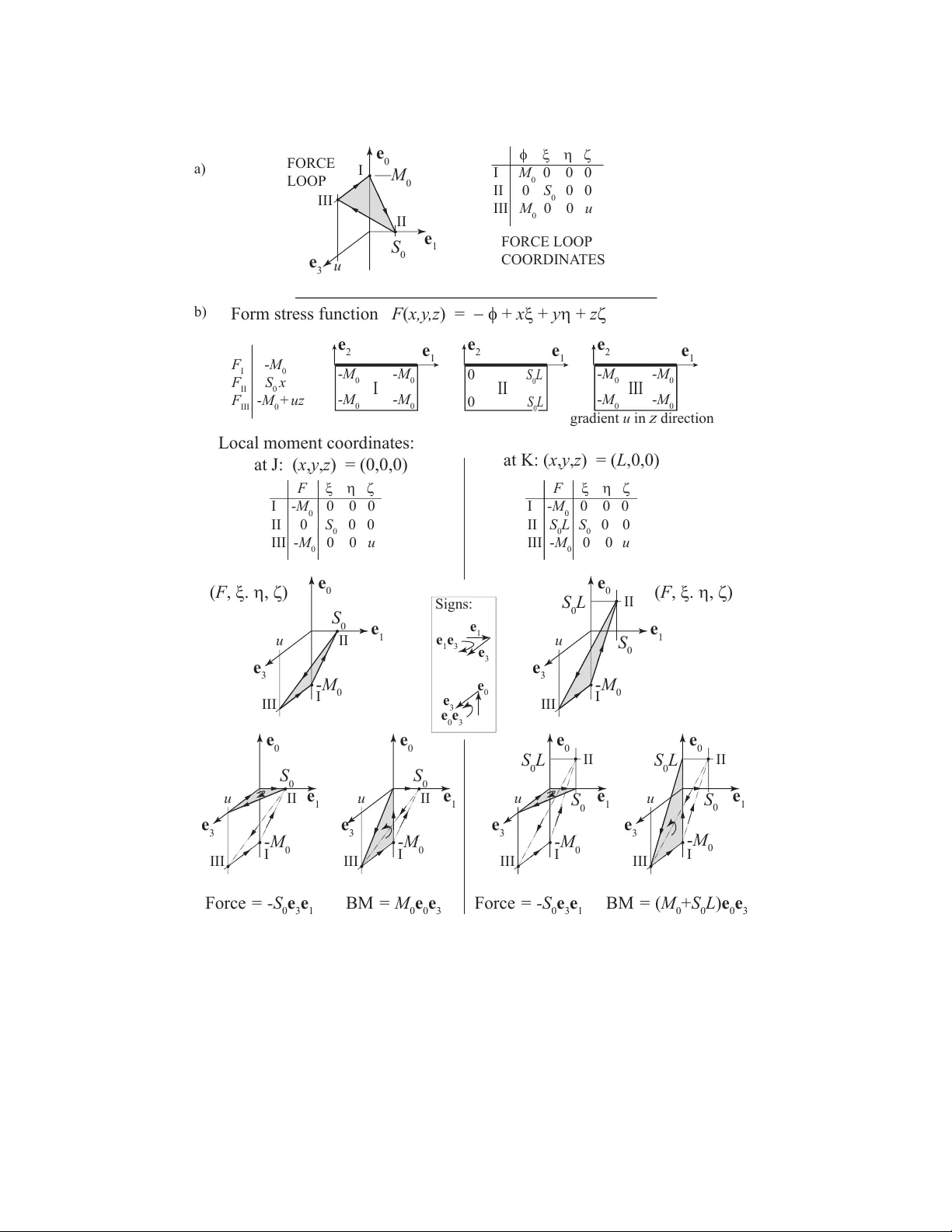
Original Paper
Loading high-quality paper...
Comments & Academic Discussion
Loading comments...
Leave a Comment