Multi-Agent Reinforcement Learning Counteracts Delayed CSI in Multi-Satellite Systems

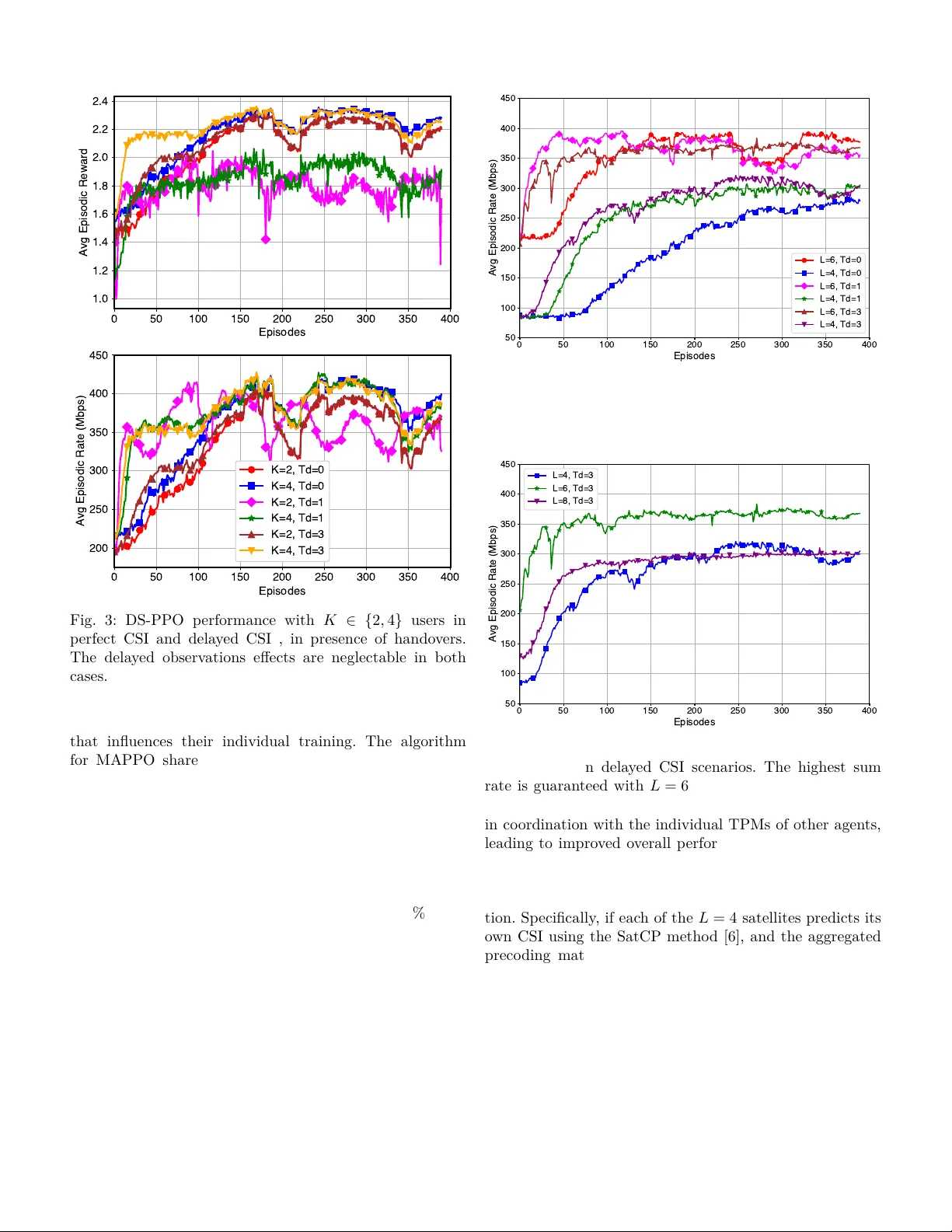
1 Multi-Agen t Reinforcemen t Learning Coun teracts Dela y ed CSI in Multi-Satellite Systems Marios Aristo demou § , Y asaman Omid ∗ , Sangarapillai Lam b otharan † , Mahsa Derakhshani ∗ , La jos Hanzo ‡ § Departmen t of Computer Science, Univ ersit y of Y ork, Y ork, U.K. ∗ W olfson Sc ho ol of Mec hanical, Electrical and Man ufacturing Engineering, Lough b orough Univ ersit y , Lough b orough, U.K. † Institute for Digital T ec hnologies, Lough b orough Univ ersit y (London Campus), London, U.K. ‡ Sc ho ol of Electronics and Computer Science, Univ ersit y of Southampton, Southampton, U.K. Abstract—The in tegration of satellite communication net- w orks with next-generation (NG) tec hnologies is a promising approac h to wards global connectivit y . Ho wev er, the quality of services is highly dep endan t on the av ailability of accurate c hannel state information (CSI). Channel estimation in satellite comm unications is c hallenging due to the high propagation dela y b et w een terrestrial users and satellites, whic h results in outdated CSI observ ations on the satellite side. In this paper, w e study the do wnlink transmission of m ultiple satellites acting as distributed base stations (BS) to mobile terrestrial users. W e propose a m ulti-agent reinforcement learning (MARL) algorithm which aims for maximising the sum-rate of the users, while coping with the outdated CSI. W e design a nov el bi-lev el optimisation, pro cedure themes as dual stage proximal policy optimisation (DS-PPO), for tac kling the problem of large contin uous action spaces as well as of indep endent and non-iden tically distributed (non-I ID) en vironments in MARL. Sp ecically , the rst stage of DS-PPO maximises the sum-rate for an individual satellite and the second stage maximises the sum-rate when all the satellites coop erate to form a distributed m ulti-antenna BS. Our n umerical results demonstrate the robustness of DS-PPO to CSI imp erfections as well as the sum-rate improv emen t attached b y the use of DS-PPO. In addition, we pro vide the conv ergence analysis for the DS-PPO along with the computational com- plexit y . Index T erms—LEO Satellite Comm unication, Non-terrestrial Net works, Outdated CSI, Multi-Agen t Reinforcemen t Learning, Distributed MIMO I. Introduction N ON-TERRESTRIAL net w orks (NTN) and particu- larly satellite communications (SatComs) are emerg- ing tec hnologies that are exp ected to nd their w ay in the next-generation (NG) comm unication systems. Low- earth orbit (LEO) satellites provide extended co verage for n umerous devices, while main taining a relativ ely lo w latency compared to geostationary satellites [ 1 ]. Examples lik e the Starlink mega-constellation are already pro viding a dense netw ork of satellites, enabling users roaming in o- the-grid areas to stay connected [ 2 ], [3]. The high-altitude platforms, such as unmanned aerial vehicles, are unable to provide contin uous, long-term connectivity . Thus, the in tegration of terrestrial netw orks with satellites is a vital step for NG systems. In tegrating SatComs with terrestrial net w orks poses signican t c hallenges in ac hieving high-throughput con- nectivit y . Some of these challenges include high Doppler shifts, frequen t satellite hando vers, and long propagation dela ys [ 4 ]. Specically , propagation delays p ose challenges for the channel estimation pro cess in the uplink, as the dela y exceeds the c hannel’s coherence in terv al. T o estimate the CSI, users transmit unique pilot sequences, allowing the satellites to estimate the c hannels betw een the tw o parties. How ev er, the propagation dela y results in a mis- matc h betw een the estimated c hannel state information (CSI) and the actual CSI. This issue is kno wn as the “outdated/dela y ed CSI problem,” whic h we aim to address. In the literature, several authors ha ve considered the eect of delay ed CSI in downlink satellite-user transmis- sion. The authors of [ 5 ] prop osed a deep learning (DL)- based satellite channel predictor that used long short-term memory units for eliminating the detrimen tal impact of the outdated CSI. In [ 6 ], a pair of deep neural netw orks (DNN) w ere prop osed, one for satellite channel prediction (SatCP) and another for satellite hybrid b eamforming (SatHB). In SatCP , the correlation b etw een the uplink and the do wnlink CSI w as exploited for predicting the downlink CSI b y a DNN. By feeding the output of the SatCP netw ork in to the SatHB net w ork, the SatHB maps the predicted CSI to a desired h ybrid b eamformer. F urthermore, in [7], an RL algorithm using the deep deterministic p olicy gradien t (DDPG) tec hnique is introduced for coping with the eects of delay ed CSI. Unlike previous researc h, in [ 7 ], the delay ed CSI is directly mapp ed to the optimised transmit preco d- ing matrix (TPM), skipping ov er the channel prediction en tirely . In LEO satellite netw orks, the dense constellation of satellites ensures that multiple satellites are visible to terrestrial users at an y given time [ 8 ]. This allows the satel- lites to op erate as a distributed m ultiple-input multiple- output (MIMO) base station (BS), providing signicant div ersit y gain to improv e the throughput, enhance reli- abilit y , and mitigate fading eects. These satellites are connected b y inter-satellite links, enabling them to share 2 their information eectiv ely [ 9 ]. T o maximise throughput, the satellites m ust collab oratively form a distributed TPM, while accoun ting for the challenges of outdated CSI. T o the b est of our knowledge, the consideration of outdated CSI in a co op erative multi-satellite system has only b een dis- cussed in [10], where the authors harnessed the statistical information of the channel estimation errors to cop e with the deleterious eects of outdated CSI. The simplicit y of the tec hnique mak es it compatible with systems having lo w op erating frequencies of up to 1 GHz. While it is theoret- ically p ossible to model such dela ys probabilistically and apply robust or sto c hastic optimisation [11], in practice, high user/satellite mobilit y and the increasing carrier fre- quency (e.g., ab ov e 1 GHz) introduce rapidly time-v arying c hannels. As shown in [10], the error induced b y delay ed CSI under these conditions becomes excessive to model accurately via a simple statistical distribution. This renders con v entional conv ex optimisation approac hes ineectiv e due to high statistical uncertaint y . F or higher op erating frequencies, the current literature of multi-satellite systems either considers the unrealistic scenario of perfect CSI or they only rely on statistical CSI. T o ll the knowledge gaps, we aim for directly mapping the delay ed CSI to an optimised TPM in a m ulti-satellite system. How ever, the tec hnique conceived in [ 7 ] cannot b e applied here due to the indep endent and non-identically distributed (non-iid) nature of the environmen t, where eac h satellite’s path uniquely determines its CSI. Hence, the RL agen t(s) must track and adapt to the dynamic c hanges across multiple channels, signicantly increasing the complexity of the task. In this pap er, we explore the p oten tial of multi-agen t reinforcemen t learning (MARL) in counteracting the outdated CSI challenge in co op erative m ulti-satellite systems, where satellites act as distributed agen ts. Our contributions are as follows: 1) W e address the c hallenge of c hannel aging in multi- satellite downlink comm unication to mobile devices. In constrast to [ 5 ], [ 6 ], our w ork bypasses channel prediction altogether by directly mapping the de- la y ed CSI to the TPMs. F urthermore, in contrast to [10], our approac h is sp ecically designed for high- frequency scenarios and incorp orates distributed TPM optimisation. This eliminates the reliance on a high- p erformance net w ork con troller and eectiv ely dis- tributes the pro cessing load across satellites. 2) W e propose a no v el algorithm termed as Dual-Stage Pro ximal Policy optimisation (DS-PPO). Unlike the metho d in [ 7 ], the DS-PPO algorithm is sp ecically de- signed for co op erative multi-satellite communications with non-iid en vironmen ts. W e introduce a bi-level optimisation framework for handling the complexity of the environmen t: In a given satellite, the rst pro ximal p olicy optimisation (PPO) optimises the satellite’s TPM to maximise its individual sum-rate. The second PPO lev erages the singular v alues of the rst stage TPM across other satellites to optimise its TPM as part of a distributed satellite system. Sharing these singular v alues limits the information exchanged among satellites, enabling them to handle the non-iid en vironmen t through distributed learning. 3) W e provide the computational complexity and the con v ergence analysis of the DS-PPO, proving that DS-PPO provides a performance impro vemen t to the global sum-rate, and that DS-PPO can b e considered as a light weigh t algorithm. 4) W e demonstrate the robustness of DS-PPO to CSI dela ys and its sup erior p erformance in handling com- plex multi-satellite scenarios through numerical ev al- uations. As for the rest of this paper, the system mo del and problem form ulation are presen ted in Section II. Section IV explains the prop osed algorithm in details. The numerical results are giv en in Section VI I, and Section VI II concludes the pap er. I I. System Mo del and Problem F orm ulation In this pap er, w e consider a dense LEO satellite con- stellation where L satellites are collab orating with each other through their in tersatellite links to provide connec- tivit y for K single-antenna mobile users on the ground. Eac h satellite is equipp ed with a uniform planar array (UP A) of M = M x × M y an tennas. Since in SatComs the c hannels mostly consist of line of sight (LOS) links, this collaboration among satellites increases the diversit y o v erall, which can enhance the system throughput. At eac h time instant, these satellites aim for transmitting a v ector of sym bols s ( t ) = [ s [1] ( t ) , ..., s [ K ] ( t )] T to the users, and they precode this data via a TPM formulated by V ( t, f ) = [ v [1] ( t, f ) , ..., v [ K ] ( t, f )] ∈ C M L × K . Note that eac h M rows of this matrix is in fact a preco ding sub-matrix for an individual satellite. In other w ords, V l ( t, f ) ∈ C M × K is a sub-TPM for the l th satellite, whic h con tains the rows [( l − 1) M + 1] to ( M l ) of the matrix V ( t, f ) . A cluster is referred to as the set of satellites that are collab orating with eac h other for data transmission and form a distributed MIMO system. W e use a LEO constellation of satellites similar to Starlink. As in any other LEO constellation, the satellites orbit the earth with a high sp eed (in the range of 7 km/sec for Starlink). This means that a given satellite has a short window of connection to a given ground user (in the range of 5 minutes). W e say a satellite is visible to a ground user when it is within the user’s 30 degree elev ation angle. At any given time, for a user lo cated in the UK, around 40 satellites are in sight. A t a giv en time t , w e select L satellites from the set of satellites that are visible to a certain cov erage region on earth, to form a cluster. These L satellites are selected based on their distance to the centre of the cov erage area, i.e. the L satellites that are closest to the cen tre of the co v erage area at time instan t t are selected to form the cluster. Ho w ev er, 3 Fig. 1: System mo del: a cluster of L satellites pro viding service for K users. due to satellites’ mobilit y , these satellites mov e aw ay from the cov erage region and they are replaced in the cluster by satellites with shorter distances to the users. This is called a satellite handov er. W e use the distance metric for satellite hando v ers rather than the received pow er or channel gain, to av oid p erforming a handov er due to short-term channel uctuations. Instead we base our handov er mechanism on the free-space path-loss (FSPL). The satellites in a cluster are aiming for optimising their lo cal TPMs in order to maximise the ov erall sum- rate. Th us, w e form our problem with the ob jectiv e of maximising the sum-rate of the users, as max V ( t,f ) K X k =1 log  1 + | h [ k ] H ( t, f ) v [ k ] ( t, f ) | 2 P K i  = k | h [ k ] H ( t, f ) v [ i ] ( t, f ) | 2 + σ 2  s.t. T r  V l ( t, f ) V H l ( t, f )  ≤ P l , l ∈ { 1 , ..., L } , (1) where h [ k ] ( t, f ) ∈ C M L × 1 is the CSI of user k , σ 2 is the v ariance of the additive white Gaussian noise at the user side, and P l is the p ow er budget for the l th satellite. In order to solve this optimisation problem, we need accurate CSI at the satellite side. The users transmit pilot sequences, so that the satellites can estimate the channels, but due to the large propagation delay , the CSI that the satellites estimate b ecome outdated. The propagation delay betw een a given user k and a satellite l is τ d ( k , l ) = d k,l c where d ( k , l ) is the distance of the tw o nodes and c is the speed of ligh t. Assuming that the pilots are transmitted every ∆ T seconds, w e could say that the CSI is delay ed for T d ( k , l ) time instances where T d ( k , l ) = ⌈ τ d ( k,l ) ∆ T ⌉ is the discrete v ersion of the delay . No w, at a given time instant t the satellite l has the CSI at t − T d ( k , l ) . by dening the dela y of the cluster of satellites as T d = max k,l ( T d ( k , l )) , we aim to design the TPMs V l ( t, f ) , ∀ l by having access to the c hannels at t − T d , e.g. h [ k ] ( t − T d , f ) , ∀ k . This is referred to as the delay ed CSI problem with constant delay . In addition, the global sum-rate optimisation problem is non-con v ex due to the structure of the rate expression. Sp ecically , the TPM v [ i ] ( t, f ) (which is an M L × 1 preco ding v ector from all satellites to the user i ) appears in b oth the n umerator and the denominator of the SINR expression, and the sum-rate is calculated across users not across the satellites, introducing coupling b et w een agen ts and dep endencies that are hard to isolate. Also, as mentioned ab ov e, the CSI a v ailable to each satellite is outdated, which can be in terpreted as a statistical p erturbation of the actual channel (similar to [10]). While it is theoretically possible to mo del such dela ys proba- bilistically and apply robust or sto chastic optimisation, in practice, high user/satellite mobility and the increasing carrier frequency (e.g., ab o v e 1 GHz) in tro duce rapidly time-v arying c hannels. As sho wn in [10], the error induced b y delay ed CSI under these conditions becomes excessiv e to mo del accurately via a simple statistical distribution. This renders conv entional conv ex optimisation approaches ineectiv e due to high statistical uncertaint y . I I I. Background and Preliminaries In the follo wing sub-sections w e review the basic prelim- inaries of our prop osed algorithm, namely the Augemen ted Mark o v Decision Pro cess (MDP) in order to tac kle the Dela y ed CSI, and the Pro ximal Policy Optimisation (PPO). Then, we discuss the limitations of other no vel algo- rithms in Multi Agen t Reinforcement Learning (MARL) in comparison to our problem formulation and enviromen tal constrain ts. A. Augmen ted Mark ov Decision Pro cess for Dela yed CSI T o address the c hallenge of dela yed information, we emplo y an augmented MDP instead of the traditional MDP . The concept of an augmented MDP w as introduced in [12], where the authors prop ose solutions for managing MDPs with constan t dela ys. Sp ecically , the authors sug- gested that, to construct an equiv alent MDP with p erfect state information, the agent’s previous actions should b e included in the state information, as { s ( t − T d ) , a ( t − T d ) , a ( t − T d + 1) , ..., a ( t − 1) } ∈ S ′ , (2) where s ( t − T d ) is the dela y ed observ ation, and a ( t − T d ) , a ( t − T d + 1) , ..., a ( t − 1) are the previous actions during the delay p erio d. B. Proximal Policy Optimisation PPO is an on-p olicy , mo del-free RL algorithm designed to take smaller steps using the most recent a v ailable data [13]. PPO addresses tw o key c hallenges: determining the appropriate step size for p olicy up dates and main taining training stability . It builds up on concepts used in trust region policy optimisation [14]. The core idea b ehind PPO is to mak e gradual impro vemen ts during p olicy up dates [13]. It has the abilit y to optimise the policy using smaller steps and conv erging faster than other methodologies, th us, 4 it is deemed for our problem formulation with a non-iid distribution and delays. PPO has a critic netw ork ( V ϕ ) to estimate the v alue function and an actor netw ork ( π θ ) that represents the p olicy that selects actions. During each iteration, the algorithm go es through a phase known as ”rollout,” where the current policy samples actions ov er T time steps and computes the rewards. At the end of the rollout, PPO calculates the adv antage using generalized adv antage estimation (GAE), which is given by ˆ A π t = δ t + ( γ λ ) δ t +1 + · · · + ( γ λ ) ( T − 1) δ T − 1 , (3) where r t is the rew ard function, γ is the discoun t factor, λ is the GAE discoun t factor and δ t is the adv antage function that estimates the adv antage of an action a in state s under p olicy π and is given by , A π ( s, a ) = Q π ( s, a ) − V π ( s ) (4) where Q π ( s, a ) = r ( s, a ) + γ E s ′ ∼ P ( ·| s,a ) [ V π ( s ′ )] is the action-v alue function. Next, the rollout data is divided into small mini-batches, whic h PPO iterates ov er for K ep o chs. During the update ep o c hs, w e calculate the ratio b etw een the new p olicy and the old policy . This ratio is then used to compute the loss for the clipp ed surrogate ob jective, which is given by L clip ( θ ) = ˆ E t [ min ( r t ( θ )) ˆ A π t , clip ( r t ( θ ) , 1 − ϵ, 1 + ϵ ) ˆ A π t ] (5) where, ϵ balances the exploration and exploitation of the clipp ed surrogate function. Then, the total loss is computed as the sum of three comp onents: the clipp ed surrogate ob jectiv e, the v alue function loss, and the entrop y b on us, whic h is given by L total = ˆ E t [ L clip ( θ ) − c 1 · L V F ( θ ) + c 2 · H ( π θ | s t )] , (6) where, c 1 , c 2 are the coecients, and H ( · ) is the entrop y function and L V F is given by L V F = ( V θ ( s t ) − V targ et t ( s t )) 2 , where V θ and V targ et are the current v alue function and the target v alue, resp ectively . W e use the combined loss in (6) in order to up date the parameters using the Adam optimiser. With this tec hnique, PPO balances exploration, stabilit y , and learning eciency . C. Limitations of Existing MARL Approaches There are sev eral prominent multi-agen t reinforcement learning algorithms, which are not directly applicable to our problem form ulation due to fundamen tal arc hitectural and en vironmen tal constrain ts [15], [16]. F or example, Multi Agen t Deep Deterministic P olicy Gradien t (MADDPG) [17] emplo ys a centralised training with decentralised execution, where eac h agent’s critic requires access to the observ ations and actions from all agen ts during training. In our LEO satellite netw ork, this would necessitate gath- ering O ( LM K ) dimensional state and action information from all L satellites at a central lo cation, incurring a large in ter-satellite communication o verhead. This becomes more problematic considering the large action space in our system. Similarly the Multi Agent Proximal P olicy Optimisation [18] relies on a centralised v alue function that conditions on global state, whic h is infeasible when satellites cannot share their full CSI in a timely manner. In QMIX (Monotonic V alue F unction F actorisation) [19] and Counterfactual Multi-Agent Policy Gradients (COMA) [20], it is assumed that there is access to a mixing net work or a centralised critic that combines individual agent util- ities, requiring sync hronous global information exchange that violates the distributed nature of our system. More- o v er, these algorithms assume stationary environmen ts where the global p olicy conv erges to a xed equilibrium. F or example, recent w ork on fully decen tralised MARL with net w ork ed agen ts [21] has established con v ergence guaran tees for actor-critic algorithms with linear function appro ximation, but assumes stationary environmen ts whic h do not apply to our scenario. In contrast, our satellite net w ork exhibits inherent non-stationarity environmen ts due to the satellite mobilit y with con tin uous hando vers and cluster reconguration, the time-v arying delay ed c hannels, and user mobility , in troducing unpredictable interference patterns. IV. Prop osed DS-PPO Algorithm In this section, we discuss the metho dology used for solving the problem in ( 1 ). By exploiting the adv an tages of PPO, we conceiv e a bi-level optimisation pro cedure for rst optimising each satellite’s individual sum rate and then optimise the ov erall sum rate for the scenario when the satellites work as a distributed MIMO. By taking into accoun t that the CSI observ ations are dela y ed, this problem b ecomes a constan t dela y Marko v decision pro cess (MDP), whic h is discussed in the follo wing sub-section. Note that the v alue of this constan t delay in observ ations is dep endent on b oth the propagation delay and on the pilot transmission rate, whic h determines the duration of each time step. A. Algorithm In our MARL mo del, each agen t represents a satellite and it is tasked with calculating the preco ding sub-matrix sp ecic to its satellite. This computation is p erformed using information shared b y other satellites within the cluster, enabling co ordinated and ecient operation. The DS-PPO MARL algorithm w e develop is a deriv ation of the PPO RL algorithm dened in [13]. Again, the prop osed algorithm op erates in t wo stages to optimise the TPM based on the dela y ed CSI for a distributed m ulti-satellite comm unication system, as shown in Figure 2 . This DS- PPO MARL algorithm is particularly useful for distributed learning scenarios where agents are dealing with non-I ID en vironmen ts. In the rst stage, the algorithm determines the initial TPM for eac h satellite, assuming that eac h satellite is transmitting to the users indep endently . W e emplo y PPO RL of [13] to optimise each satellite’s sum-rate based on its 5 Fig. 2: DS-PPO for enhanced TPM generation. o wn CSI and rew ard structure. Next, the algorithm calcu- lates the singular v alues of the individual TPMs obtained in the rst stage. These singular v alues are then shared among the satellites in the cluster, pro viding compact and meaningful information ab out each satellite’s transmission c haracteristics. This stage helps reduce the dimensionality of the information exc hanged among satellites, making the pro cess more ecient. Additionally , in the rst stage of DS-PPO, sharing singular v alues enables eac h satellite to assess how muc h p ow er other satellites are allo cating to eac h user individually . This helps the agents to track the pattern of changes in the CSI of each satellite. In the second stage, the algorithm up dates the TPMs by incorp orating the shared singular v alues and the dela yed CSI, treating the satellites as part of a distributed MIMO system. An additional agent is trained for each satellite using the second stage of PPO, aiming for maximising the global sum-rate for the en tire satellite net w ork. This co op erativ e update allows the system to trac k satellite mo v ements and adapt to c hanges in the CSI, impro ving the o v erall transmission p erformance. The DS-PPO metho d is giv en in Algorithm 1 . B. State Space Due to the fact that there are t w o dierent stages in DS-PPO, w e dene tw o dieren t state spaces and rew ard functions. The state space in the rst stage uses the augmented state from Section I I I-A. T o reduce b oth the computational complexity and the resources in each satellite, w e hav e selected the pilot transmission rate for ensuring that the CSI observed would hav e only a single time step transmission delay . In other words, the time duration b et w een tw o consecutive CSI observ ations matc hes the propagation delay of the environmen t. Thus, the state space of the rst stage s l t, 1 at time step t for the l -th satellite is s l t, 1 = { H l ( t − T d , f ) , V l ( t − T d , f ) } where H l ( t − T d , f ) ∈ C M × K , is the outdated CSI of the l th satellite, while, the V l ( t − T d , f ) is its TPM. Algorithm 1: DS-PPO Algorithm for MARL Input : CSI H Output: Optimal TPMs V ′ 1 for iteration = 1, 2, ... do 2 for t = 1, ..., T do 3 V ← First Stage Agen ts ( H ) 4 Calculate Reward for ( V , H ) 5 Find the singular v alues of V to form Λ 6 V ′ ← Second Stage Agents ( V , Λ) 7 end 8 P erform PPO T raining for b oth stages 9 end The second stage uses the action from the previous stage and the singular v alues from the other satellites. Therefore, the state space s t, 2 of the second stage is dened as, s l t, 2 = { V l ( t − T d , f ) , Λ l } , Λ l = L [ j  = l λ j , λ j ∈ R 1 × K where Λ l is the set of all singular v alues of V ′ l ( t − T d , f ) , ∀ l ′  = l gleaned from the other satellites in the cluster. C. Action Space The action space is a contin uous space, dened by the real and imaginary comp onents of the TPM co ecients. Th us, its dimensionalit y is determined b y 2 K M . The action spaces for the rst and second stages at time step t for the l th satellite are denoted by , Stage 1: a l t, 1 = { V l ( t, f ) } Stage 2: a l t, 2 = { V ′ l ( t, f ) } D. Reward function F or each stage we use t wo dieren t rew ard function. The rst stage reward function is aiming to help the agen ts to learn and optimise the TPM individually in order to maximise their sum rate and the second stage rew ard function to incorp orate the optimisation ob jectiv e to optimise the TPM collab oratively . 1) First Stage: Our rew ard function consists of three comp onen ts: f ( · ) , which is associated with the curren t sum- rate; g ( · ) , which considers b oth the current and past sum- rates; and a term represen ting the p ow er constrain t. The rew ard r l t for the rst stage of PPO, at time step t for the l -th satellite is giv en by r l t = f ( c t ) + g ( c t , c t − 1 ) − p l (7) 6 where c t is the sum rate of users at time t in case only the satellite l is providing service for the users individually . The functions f ( c t ) , g ( c t , c t − 1 ) , and p l are denoted by f ( c t ) =                          − 2 , c t ≤ ξ 1 − 1 , ξ 1 < c t ≤ ξ 2 0 , ξ 2 < c t ≤ ξ 3 1 , ξ 3 < c t ≤ ξ 4 2 , ξ 4 < c t ≤ ξ 5 2 + ⌈ c t ⌉ − ξ 5 , c t > ξ 5 (8) g ( c t , c t − 1 ) = sign ( c t − c t − 1 ) · 1 . 5 − 0 . 5 , (9) p l = 3 10   tr  V l ( t, f ) · V l ( t, f ) H  − P l   , (10) with P l represen ting the p ow er budget for the l th satellite. Note that in order for the agent in satellite l to calculate c t for the second stage, all satellites in the cluster need to share their CSI observ ations and their nal preco ding matrices with each other. The rst part of the reward function f ( c t ) is designed in a quan tized form to support the learning pro cess of the RL agen ts. The c hoice of h yp erparameters for this quan tization was guided b y the target sum-rate we wan ted to ac hieve. In particular, our goal w as to ensure a minim um guaran teed sum-rate of around 300 Mbps, and thus the follo wing parameters in T able I . Besides fo cusing on the sum-rate itself, w e also tak e into account whether the sum-rate has improv ed during training. F or this, we use the function g ( c t , c t − 1 ) which simply adds or subtracts a constan t from the reward dep ending on whether the sum- rate has increased compared to the previous time step. Finally , to regulate the p ow er consumption of the TPM, w e include the term p l . ξ 1 ξ 2 ξ 3 ξ 4 ξ 5 120 5 ξ 1 4 = 150 7 ξ 1 4 = 210 9 ξ 1 4 = 270 3 ξ 1 = 360 T ABLE I: P arameters used in f ( c t ) , that ensure a minim um guaran teed sum-rate of around 300 Mbps Note that in (4), with the P l , we represen t the pow er budget for the l th satellite to regulate the p ow er consump- tion of the TPM. The addition of p ow er constrain t p l aims to optimise the TPM suc h that to main tain the TPM inside the feasibilit y region. T o guaran tee this w e hav e project the predicted TPM V l in to a sphere of radius P [ 7 ]. Prop osition 1 (P o wer Budget Projection). Given the TPM V l , the pro jection of V l in to a set S is given by , min P ∈ S ∥ V l − P ∥ (11) Giv en that S is a sphere centred at the origin with radius P , such that ( S = { V l |∥ V l ∥ ≤ P } ) , the pro jection of V l is obtained b y P × V l ∥ V l ∥ + max(0 , P − ∥ V l ∥ ) (12) 2) Second Stage: The reward function for the second stage is a simplied representation of our ob jective, in- corp orating the logarithm of the sum-rate of users b eing serv ed by the satellite cluster, denoted as c ′ t , and the p ow er constrain t p l , giv en by r t = ( log ( c ′ t ) − p l − 1 , c ′ t − 1 > c ′ t , log ( c ′ t ) − p l + 1 , c ′ t − 1 < c ′ t . . (13) Note that the logarithmic function is used here to constrain the v ariations in the rew ard function, ensuring more stable and manageable up dates during optimisation. V. Conv ergence Analysis In this section, we provide the con v ergence analysis for the DS-PPO. Our conv ergence analysis builds upon the p olicy mirror descent framework [22], which establishes linear conv ergence rates for p olicy optimisation metho ds. Giv en the fact that capacit y depends on the state of Stage 1, and action of State 2, we ha v e considered how the action of Stage 2 conv erged to the optimal solution T o recap, we mo del each satellite’s decision pro cess as a Marko v Decision Process (MDP) M = (S , A , P , r, γ , ρ 0 ) where S is the state space, A is the action space, P : S × A → ∆(S) is the transition kernel, r : S × A → R is the rew ard function, γ ∈ [0 , 1) is the discount factor, and ρ 0 ∈ ∆(S) is the initial state distribution [23]. Also, note that π 1 and π 2 are the policies for the rst and second stage, resp ectively . Our analysis follows the framework established in [24] for analysing p olicy gradient conv ergence. The following denitions are imp ortant for the conv ergence analysis and pro v e that stage 2 conv erges to an optimal solution. Denition 1 (P olicy Performance). The exp ected cumula- tiv e discounted reward under p olicy π is: η ( π ) = E τ ∼ π " ∞ X t =0 γ t r ( s t , a t ) # = E s 0 ∼ ρ 0 [ V π ( s 0 )] (14) where V π ( s ) = E π [ P ∞ t =0 γ t r ( s t , a t ) | s 0 = s ] is the v alue function. Denition 2 (Adv an tage F unction). The adv antage of ac- tion a in state s under p olicy π is: A π ( s, a ) = Q π ( s, a ) − V π ( s ) (15) where Q π ( s, a ) = r ( s, a ) + γ E s ′ ∼ P ( ·| s,a ) [ V π ( s ′ )] is the action-v alue function. W e make the following assumptions in order establish sev eral technical lemmas that will b e used in order to pro vide the upp er b ound the p olicy improv ement. Assumption 1 (Bounded Rewards). There exists R max > 0 suc h that | r ( s, a ) | ≤ R max for all ( s, a ) ∈ S × A . Assumption 2 (Lipschitz Policy). Given the p olicy π θ is Lipsc hitz contin uous in parameters, there exists L π > 0 suc h that for all s ∈ S : ∥ π θ 1 ( ·| s ) − π θ 2 ( ·| s ) ∥ 1 ≤ L π ∥ θ 1 − θ 2 ∥ (16) 7 Assumption 3 (Learning Rate Conditions). The learning rates { α n } n ≥ 0 and { β n } n ≥ 0 for Stage 1 and Stage 2 satisfy the following conditions: • α n , β n > 0 for all n • P ∞ n =0 α n = P ∞ n =0 β n = ∞ • P ∞ n =0 α 2 n < ∞ and P ∞ n =0 β 2 n < ∞ Based on the ab ov e assumptions, we hav e express the follo wing. Theorem 1 (Stage 2 P erformance Improv emen t). Let π 1 b e the conv erged Stage 1 p olicy and π 2 the Stage 2 p olicy obtained by DS-PPO. Under Assumptions 1 – 2 : η ( π 2 ) ≥ η ( π 1 ) − 4 ϵ max γ (1 − γ ) 2 · D max T V ( π 1 , π 2 ) 2 (17) where ϵ max = max s,a | A π 1 ( s, a ) | ≤ 2 R max 1 − γ is the maximum adv antage, and D max T V ( π , π ′ ) = max s D T V ( π ( ·| s ) ∥ π ′ ( ·| s )) is the maximum total v ariation divergence. The ab ov e theorem is consistent with recent results on p olicy gradien t metho ds [25] A. Preliminaries Before expressing the upp er b ound for conv ergence analysis [26], we hav e established the following lemmas. Lemma 1 (Bounded V alue F unction [25], [26]). Under Assumption 1 , for any p olicy π : | V π ( s ) | ≤ R max 1 − γ , | Q π ( s, a ) | ≤ R max 1 − γ , (18) | A π ( s, a ) | ≤ 2 R max 1 − γ for all s ∈ S and a ∈ A . Lemma 2 (Performance Dierence Lemma [27]). F or an y t w o p olicies π and ˜ π : η ( ˜ π ) = η ( π ) + E τ ∼ ˜ π " ∞ X t =0 γ t A π ( s t , a t ) # (19) where the exp ectation is o v er tra jectories τ = ( s 0 , a 0 , s 1 , a 1 , . . . ) with s 0 ∼ ρ 0 , a t ∼ ˜ π ( ·| s t ) , and s t +1 ∼ P ( ·| s t , a t ) . Lemma 3 (Discounted State Visitation). Dene the dis- coun ted state visitation frequency under p olicy π as: ρ π ( s ) = (1 − γ ) ∞ X t =0 γ t P ( s t = s | π, s 0 ∼ ρ 0 ) (20) Then ρ π is a v alid probability distribution o ver S , and the p erformance dierence can b e written as: η ( ˜ π ) − η ( π ) = 1 1 − γ X s ρ ˜ π ( s ) X a ˜ π ( a | s ) A π ( s, a ) (21) Lemma 4 (Coupling Lemma [28]). F or an y t w o probabilit y distributions p and q ov er a nite set X with total v ariation distance D T V ( p ∥ q ) = 1 2 P x | p ( x ) − q ( x ) | = α , there exists a join t distribution ( X , Y ) with marginals X ∼ p and Y ∼ q suc h that: P ( X  = Y ) = α = D T V ( p ∥ q ) (22) B. Pro of of Theorem 1 The pro of follows the approach of Sch ulman et al. [14] with detailed exp osition. W e rst b egin to dene the surrogate ob jective from the PPO. F rom Lemma 2 , the p erformance of π 2 relativ e to π 1 is: η ( π 2 ) = η ( π 1 ) + E τ ∼ π 2 " ∞ X t =0 γ t A π 1 ( s t , a t ) # (23) The dicult y is that the exp ectation is ov er tra jectories from π 2 , whic h we are trying to optimise. W e instead dene a surrogate ob jective that uses tra jectories from π 1 : L π 1 ( π 2 ) = η ( π 1 ) (24) + E τ ∼ π 1 " ∞ X t =0 γ t π 2 ( a t | s t ) π 1 ( a t | s t ) A π 1 ( s t , a t ) # Using Lemma 3 , this can b e written as: L π 1 ( π 2 ) = η ( π 1 ) (25) + 1 1 − γ X s ρ π 1 ( s ) X a π 2 ( a | s ) A π 1 ( s, a ) Here the key observ ation is when π 2 = π 1 , meaning that there is no improv ement o v er the baseline p olicy (Stage 1), by denition, adv an tage b ecomes zero, b ecause the exp ected adv antage of a p olicy o v er itself is alwa ys zero. Therefore, L π 1 ( π 1 ) = η ( π 1 ) (26) Also, at this p oint, the gradient will match as b elow, ∇ π 2 L π 1 ( π 2 )    π 2 = π 1 = ∇ π 2 η ( π 2 )    π 2 = π 1 (27) This means the surrogate L π 1 is a rst-order appro xima- tion to η around π 1 . The next step in the pro of is to b ound the gap b etw een η ( π 2 ) and L π 1 ( π 2 ) . The gap arises b ecause the η ( π 2 ) uses state visitation ρ π 2 and the L π 1 ( π 2 ) uses state visitation ρ π 1 . W e rst need to dene the exp ected adv an tage under π 2 at state s : ¯ A π 1 ( s ) = E a ∼ π 2 ( ·| s ) [ A π 1 ( s, a )] (28) = X a π 2 ( a | s ) A π 1 ( s, a ) F rom Lemma 3 we can express the dierence b etw een t w o p olicies such as: η ( π 2 ) − L π 1 ( π 2 ) = (29) 1 1 − γ X s ( ρ π 2 ( s ) − ρ π 1 ( s )) ¯ A π 1 ( s ) 8 W e no w b ound | ρ π 2 ( s ) − ρ π 1 ( s ) | using coupling argu- men ts. First, let α = D max T V ( π 1 , π 2 ) = max s D T V ( π 1 ( ·| s ) ∥ π 2 (30) By Lemma 4, at each state s , w e can couple the actions under π 1 and π 2 suc h that they dier with probability at most α . W e consider that there are tw o tra jectories: • τ (1) = ( s 0 , a 0 , 1 , s 1 , 1 , a 1 , 1 , . . . ) with a t, 1 ∼ π 1 ( ·| s t, 1 ) • τ (2) = ( s 0 , a 0 , 2 , s 1 , 2 , a 1 , 2 , . . . ) with a t, 2 ∼ π 2 ( ·| s t, 2 ) starting from the same initial state s 0 . Using the coupling, w e can ensure that at each step, given the tra jectories hav e not div erged: P ( a t, 1  = a t, 2 | s t, 1 = s t, 2 ) ≤ α Let T be the rst time the tra jectories div erge (i.e., a t, 1  = a t, 2 or equiv alently s (1) T +1  = s (2) T +1 ). Then: P ( T > t ) = P ( tra jectories identical up to time t ) ≥ (1 − α ) t Therefore, the probability that the trajectories hav e div erged by time t is: P ( T ≤ t ) ≤ 1 − (1 − α ) t (31) Using the inequality 1 − (1 − α ) t ≤ tα for α ∈ [0 , 1] : P ( s t, 1  = s t, 2 ) ≤ tα (32) No w we need to nd a relationship in order to b ound correctly the state visitation dierence. F or any function f : S → R with | f ( s ) | ≤ f max : | E s t ∼ π 2 [ f ( s t )] − E s t ∼ π 1 [ f ( s t )] | = | E [ f ( s t, 2 ) − f ( s t, 1 )] | = | E [ f ( s t, 2 ) − f ( s t, 1 ) | s t, 1  = s t, 2 ] · P ( s t, 1  = s t, 2 ) | + | E [ f ( s t, 2 ) − f ( s t, 1 ) | s t, 1 = s t, 2 ] · P ( s t, 1 = s t, 2 ) | ≤ 2 f max · P ( s t, 1  = s t, 2 ) + 0 (33) ≤ 2 f max · tα (34) Applying this with f ( s ) = ¯ A π 1 ( s ) and f max = ϵ max = max s,a | A π 1 ( s, a ) | :   E s t ∼ π 2 [ ¯ A π 1 ( s t )] − E s t ∼ π 1 [ ¯ A π 1 ( s t )]   ≤ 2 ϵ max · tα (35) If w e go through the summation o ver time w e can nd a b ound. | η ( π 2 ) − L π 1 ( π 2 ) | =      ∞ X t =0 γ t  E s t ∼ π 2 [ ¯ A π 1 ( s t )] − E s t ∼ π 1 [ ¯ A π 1 ( s t )]       ≤ ∞ X t =0 γ t · 2 ϵ max · tα = 2 ϵ max α ∞ X t =0 tγ t (36) W e compute the sum P ∞ t =0 tγ t . Let S = P ∞ t =0 tγ t . Then: S = 0 + γ + 2 γ 2 + 3 γ 3 + · · · γ S = γ 2 + 2 γ 3 + 3 γ 4 + · · · S − γ S = γ + γ 2 + γ 3 + · · · = γ 1 − γ S = γ (1 − γ ) 2 Therefore if substitute the ab ov e into 35 | η ( π 2 ) − L π 1 ( π 2 ) | ≤ 2 ϵ max α · γ (1 − γ ) 2 = 2 ϵ max γ α (1 − γ ) 2 (37) The b ound (37) is linear in α , and while mathematically v alid, a linear b ound is insucient for guaran teeing p olicy impro v ement, thus we need rene α for a quadratic. F ollowing [14], we use the fact that for small α : 1 − (1 − α ) t ≤ min(1 , tα ) (38) F or the coupled trajectories, the probability of div ergence b y time t satises: P ( T ≤ t ) = 1 − (1 − α ) t +1 ≤ ( t + 1) α (39) A more careful analysis in [14] (Appendix) shows that w e can obtain a quadratic form of α th us: | η ( π 2 ) − L π 1 ( π 2 ) | ≤ 4 ϵ max γ (1 − γ ) 2 α 2 (40) The PPO’s up date maximises the surrogate ob jective L π 1 ( π 2 ) o ver p olicies π 2 . Since the Stage 2 up date seeks to impro v e the surrogate: L π 1 ( π 2 ) ≥ L π 1 ( π 1 ) = η ( π 1 ) (41) Com bining with (40): η ( π 2 ) ≥ L π 1 ( π 2 ) − 4 ϵ max γ (1 − γ ) 2 α 2 (42) ≥ η ( π 1 ) − 4 ϵ max γ (1 − γ ) 2 α 2 (43) With substituting α = D max T V ( π 1 , π 2 ) completes the pro of. C. Remarks The analysis ab o v e inv olv es A π 1 ( s, a ) rather than A π 2 ( s, a ) . This follows directly from the P erformance Dif- ference Lemma, which states that for any t w o p olicies π and ˜ π : η ( ˜ π ) = η ( π ) + E τ ∼ ˜ π " ∞ X t =0 γ t A π ( s t , a t ) # . (44) Th us, the adv antage function is alwa ys ev aluated with resp ect to the baseline p olicy π , not the new p olicy ˜ π . This is b ecause A π ( s, a ) = Q π ( s, a ) − V π ( s ) measures how muc h b etter action a is compared to the av erage p erformance under π . T o ev aluate the improv ement of π 2 o v er π 1 , we m ust use π 2 ’s actions against π 1 ’s v alue function which 9 quan ties the impro v emen t relativ e to π 1 . Using A π 2 will pro vide no information ab out the improv ement of π 2 o v er π 1 . Thus, ¯ A π 1 ( s ) captures the exp ected b enet of following π 2 ’s action selection while measuring p erformance gains relativ e to the Stage 1 baseline. Also, note that the ab ov e analysis is to pro v e that there is a low er b ound of π 2 ’s improv ement o v er π 1 and it has not implemented as describ ed ab ov e. VI. Computational Complexity This section analyses the oating-p oint operations (FLOPS) required by DS-PPO. W e follow standard con- v en tions for counting op erations in neural net works and matrix computations [29], [30]. F or matrix op erations, w e use established results from n umerical linear algebra [30]. The matrix multiplication of C = AB where A ∈ R m × n and B ∈ R n × p requires 2 mnp FLOPS. Eac h of the mp output elemen ts requires n m ultiplications and n − 1 additions). F or a neural netw ork la y er with input dimension d in , output dimension d out , and batc h size B , the forward pass requires 2 B · d in · d out FLOPS, while the backw ard pass for computing the gradients with resp ect to b oth weigh ts and inputs, requires double the amoun t of the forward pass computation [29]. Th us, for an MLP with ℓ hidden lay ers, input dimension d in , and output dimension d out , the total forward pass FLOPS are: F MLP forward = 2 d in · d h 1 + ℓ − 1 X i =1 d h i · d h i +1 + d h ℓ · d out ! (45) The backw ard pass requires appro ximately 2 × the forward pass FLOPS [29], giving a total of F MLP train ≈ 3 · F MLP forward for one training iteration. In our implemen tation, the actor net w ork uses three la yers with 64 neurons each, while the critic netw ork uses lay ers of 128, 64, and 64 neurons. F or DS-PPO, the input/output dimensions are deter- mined by system parameters: Stage 1: d (1) in = 4 M K, d (1) out = 2 M K (46) Stage 2: d (2) in = 2 M K + ( L − 1) K , d (2) out = 2 M K (47) where the Stage 1 input is the complex CSI (real and imag- inary parts) and the past action, and Stage 2 additionally receiv es ( L − 1) K singular v alues Λ l from other satellites. The SVD of a complex M × K matrix requires appro xi- mately F SVD ≈ 8 M K 2 FLOPS [30]. The complexit y for eac h time and single satellite F step is giv en by , F step = F (1) actor + F (1) critic + F SVD + F (2) actor + F (2) critic F (1) = F (1) actor + F (1) critic F (2) = F (2) actor + F (2) critic where, F (1) actor is the Stage 1 actor netw ork, F (1) critic is the Stage 2 critic netw ork, F SVD is singular v alues decomp osi- tion, F (2) actor is the Stage 2 actor netw ork, F (2) critic is the Stage 1 critic net w ork, F (1) is the Stage 1 net w orks and F (2) is the Stage 2 netw orks. F or the total episo de that combines rollout and training is given by , F epis = T · L · F step | {z } rollout + 3 · T · L ·  E (1) · F (1) + E (2) · F (2)  | {z } training (fwd + b wd) (48) where T is the total amount of time steps, and E (1) , E (2) are the lo cal ep o c hs for stage 1 and stage 2 resp ectively . Com bining all comp onents, the total training complexit y scales as: F total = O ( N ep · T · L · ( d h · M K + d h · LK + ℓ · d 2 h + M K 2 )) (49) where N ep is the n um b er of episo des. F or xed netw ork arc hitecture ( d h , ℓ constant), this simplies to: F total = O ( N ep · T · L · K · ( M + L + K )) (50) The dominant terms are: linear in L (satellites), linear in M (antennas), and quadratic in K (users) due to SVD. F or small K , the neural netw ork terms O ( M K + LK ) dominate; for large K , the SVD term O ( M K 2 ) becomes signican t. In T able II, we summarise the FLOPS for dieren t congurations, sho wing how complexit y scales with L and K . The dominant cost is neural netw ork training (forward + bac kward passes), accounting for o ver 99% of total FLOPS. The SVD computation contributes less than 1%. T ABLE II: FLOPS Analysis for DS-PPO ( M = 9 , T = 512 , 389 episo des, 200K samples) L K Per-Episode (GFLOPS) T otal T raining (TFLOPS) 4 2 1.7 0.66 4 4 2.9 1.13 4 6 4.3 1.67 6 2 2.6 1.01 6 4 4.5 1.75 6 6 6.7 2.61 20 30 368 143.2 VI I. Numerical Results In this section, we presen t our n umerical results to ev aluate the p erformance of the prop osed DS-PPO MARL algorithm. W e incorp orate a four-la y er constellation of 4236 LEO satellites modelled after Starlink, eac h equipped with a UP A of M = 9 antennas. The constellation details are provided in [7]. In this constellation, at each instan t, sev eral satellites are visible to an y user on the ground. The cen ter of the cov erage area on Earth has the latitude of 54 . 5260000 ◦ and the longitude of − 3 . 3000000 ◦ , and the radius of the area is 50 km. A num b er of K ∈ { 2 , 4 , 6 } single-an tenna users are randomly lo cated, and they mov e in arbitrary directions with v arious sp eeds of up to 3 m/s. W e select the L ∈ { 4 , 6 , 8 } nearest satellites to the centre of the cov erage area to form a cluster. As time passes and the satellites mo v e in their orbit, some of the satellites in 10 the cluster may distance themselves from the users and giv e their p osition in the cluster to another satellite. The transmission frequency is set to f = 2 GHz, the bandwidth is set to B W = 0 . 02 f , and the channel mo del is the same as in [ 7 ]. The propagation delay is in the range of 2 . 5 msec based on the sp ecic frequency and constellation used. Note that, the delay is given by the satellite that has the longest distance from the users, b ecause the signal transmission should be p erformed sync hronously . In our study , the pilots are transmitted ev ery ∆ t = 1 ms; thus, the environmen t exp eriences a delay of T d = 3 time steps. Both stages of PPO are run with identical parameters for all agents. The actor netw ork uses the default neural net- w ork arc hitecture for PPO, and a Multi-La y er P erceptron (MLP) consisting of three lay ers with 64 neurons each. The critic netw ork has b een mo died to include three la y ers of 128, 64, and 64 neurons, respectively . Both stages share this net w ork structure and they use the ADAM optimiser. The h yp erparameters for the rst and second stages of PPO are listed in T able I I I, and they closely follow the guidelines of [31] with minimal deviations. T ABLE I I I: PPO Hyp er Parameters Parameters Symbol First Stage Second stage Discount F actor γ 0.99 0.95 GAE λ 0.95 0.9 Learning Rate η 0.003 0.004 Minibatches γ 32 6 Clip co ecien t ϵ 0.1 0.01 Maximum Gradient Norm ∥∇ s,a ∥ 1 0.6 V alue function co ecient c 1 0.1 0.01 Entrop y co ecient c 2 0.001 0.1 Epo chs N 30 10 Time steps T 512 512 A. DS-PPO Performance In order to understand and ev aluate the performance of DS-PPO, w e ha v e run experiments in four dierent settings. Sp ecically , we ev aluate the p erformance of the DS-PPO in a system of L = 4 satellites supporting K ∈ { 2 , 4 } users and in the context of p erfect CSI with no observ ation delays ( T d = 0 ) and delay ed CSI ( T d = 1 and T d = 3 ). Fig. 3 shows the av erage episo dic rate and demonstrates that the episo dic rate in the p erfect CSI scenario is that for the dela y ed CSI. Ho w ev er, the gap b et w een the perfect and delay ed CSI scenarios is negligible, whic h shows the robustness of the algorithm to the delays in CSI observ ations. In addition, for all the scenarios, the algorithm provides a minimum guaranteed sum rate of 300m bps just after the 100th episo de. The eect of hando v ers is also shown in this gure, represen ted b y the p erio dic dips in p erformance. The hando v er eect on throughput is studied in [ 7 ] in more details. Note that as more users are served, the in ter-user in terference increases, leading to a reduction in the rate p er user. How ever, this is oset by an o v erall increase in the sum-rate of all users. In the algorithmic design, though, there are signicant implications that ha v e to be considered, such as the size of the action space, which grows by 2M with the addition of eac h user. B. DS-PPO with v arying amoun t of satellites Another imp ortant study constructed for multi-satellite systems is understanding the impacts of increasing the n um b er of satellites on the sum-rate. In Fig. 4 , we c haracterize the p erformance of DS-PPO in p erfect CSI ( T d = 0 ) and dela y ed CSI ( T d = 1 , 3 ) scenarios along with L ∈ { 4 , 6 } satellites. It is evident that in b oth the scenarios of p erfect and delay ed CSI, the additional satellites hav e helped increase the a v erage episo dic sum rate due to the increased diversit y . In addition, in the scenarios of L ∈ { 4 , 6 } satellites, the delay ed CSI scenarios ha v e achiev ed a similar av erage episo dic sum rate as in the case of p erfect CSI, recording evidence that DS-PPO can cop e with the delay ed environmen t. In the case of p erfect CSI with L = 4 satellites, the agent displays shallow learning, resulting in a degraded p erformance, but, at the con v ergence stage w e can see that all three cases ac hiev e almost the same sum rate. This phenomenon is eviden tly asso ciated with the PPO’s sensitivit y to the h yp erparam- eters [31], meaning that the second stage migh t require tuning the hyperparameters to achiev e b etter results. C. DS-PPO’s empirical degree of freedom In this section, w e wan t to understand where DS-PPO ac hiev es its maximum p erformance and identify what im- pro v ements are needed to further enhance its eectiveness. In Fig. 5 , w e ev aluate the p erformance of DS-PPO in the delay ed CSI ( T d = 3 ) scenario in a system with L = 4 , 6 , 8 satellites and K = 6 users. The sum rate is generally exp ected to increase b y having more satellites in the system, due to the added div ersit y . This is shown when w e increase L = 4 to L = 6 . How ever, as shown in this gure, w e see a 25% fall in the sum rate when w e increase the num b er of satellites to L = 8 . This is as a result of the added complexit y to the agents. As we increase L , the patterns of change in the ov erall CSI, driven b y the mo vemen ts of the satellites, b ecome more signican t, making the en vironmen t increasingly non- iden tically distributed. Our DS-PPO algorithm is capable of handling this added complexity up to a certain p oint. Ho w ever, b eyond that, the complexity b ecomes to o great to manage eectiv ely . In other words, as the num b er of satellites grows, the optimisation problem faced by each agen t b ecomes more c hallenging, which in turn impacts the p erformance of the second stage of PPO. D. DS-PPO vs Other Algorithms Finally , we compare the prop osed DS-PPO MARL metho d, to other algorithms suc h as MARL with individual learning PPO (IPPO) [18]. The agents in IPPO share only rew ards betw een eac h other but no other information 11 0 50 100 150 200 250 300 350 400 Episodes 1.0 1.2 1.4 1.6 1.8 2.0 2.2 2.4 Av g Episodic Reward 0 50 100 150 200 250 300 350 400 Episodes 200 250 300 350 400 450 A g Episodic Rat e (Mb ps) K=2, Td=0 K=4, Td=0 K=2, Td=1 K=4, Td=1 K=2, Td=3 K=4, Td=3 Fig. 3: DS-PPO p erformance with K ∈ { 2 , 4 } users in p erfect CSI and delay ed CSI , in presence of handov ers. The delay ed observ ations eects are neglectable in b oth cases. that inuences their individual training. The algorithm for MAPPO shared information b etw eeen the actor and critic v alues whic h we deemed that this can increase the comm unication o verhead b etw een the agen ts, and thus, we ha v e used the IPPO which shares only the rewards. In Figure 6 , we show the results for a system of L = 4 satellites and K = 4 users. It is apparent from this gure that the DS-PPO MARL scheme ac hiev es more than 75% higher sum rate than the IPPO MARL, with an ac hiev ed a v erage sum rate of 350 Mbps and v ariance of 15%. This v ariation of the sum rate is caused by the o ccurrence of hando v ers. The results pro ve the expectation that MARL- IPPO will ha v e diculties in optimising the netw ork due to the very large action space ( 2 M K = 72 ) without the help of bi-level optimisation. Even though we use a global rew ard, whic h we exp ect to assist the PPO to learn and increase the sum-rate, the sum-rate is low er than the exp ectation. The DS-PPO oers an adv an tage by enabling the sharing of not only the rewards but also the singular v alues of the individual TPMs. This shared information allo ws the second stage of eac h agent to optimise its TPM 0 50 100 150 200 250 300 350 400 Episodes 50 100 150 200 250 300 350 400 450 Avg Episodic Ra te (Mbps) L=6, Td=0 L=4, Td=0 L=6, Td=1 L=4, Td=1 L=6, Td=3 L=4, Td=3 Fig. 4: Comparativ e results with L ∈ { 4 , 6 } satellites and K = 6 users in p erfect CSI and delay ed CSI scenarios.The incremen t in satellites clearly increases the sum rate by 20% 0 50 100 150 200 250 300 350 400 Episodes 50 100 150 200 250 300 350 400 450 Avg Episodic Ra te (Mbps) L=4, Td=3 L=6, Td=3 L=8, Td=3 Fig. 5: Comparative results with L ∈ [4 , 8] satellites and K = 6 users in delay ed CSI scenarios. The highest sum rate is guaranteed with L = 6 in co ordination with the individual TPMs of other agen ts, leading to improv ed ov erall p erformance. In this gure, we also compare our prop osed DS-PPO metho d—whic h b ypasses explicit channel estimation—with other approaches that rely on CSI prediction and estima- tion. Specically , if each of the L = 4 satellites predicts its o wn CSI using the SatCP metho d [ 6 ], and the aggregated preco ding matrix is calculated using the metho d of [10], the resulting sum rate is approximately 100 Mbps. This is only ab out one-third of the performance ac hiev ed by our DS-PPO metho d. VI I I. Conclusions W e hav e prop osed a nov el multi-agen t reinforcemen t learning algorithm termed as DS-PPO, which aims for maximising the sum-rate of a distributed multi-satellite 12 50 100 150 200 250 300 Episodes 50 100 150 200 250 300 350 400 450 500 Avg. Episodic Sum-Rate (Mbps) MARL, DS-PPO, delayed CSI MARL, IPPO, delayed CSI Channel prediction in [6] and multi-satellite precoding in [8], Perfect CSI Channel prediction in [6] and multi-satellite precoding in [8], Imperfect CSI Fig. 6: Comparative results with other algorithms. system. Our approach aims to enhance MARL algorithms to eectively handle complex environmen ts c haracterized b y div erse dynamic patterns, non-i.i.d. b eha vior, and large con tin uous action spaces, as commonly found in m ulti- satellite systems. A dditionally , we hav e pro vided a poten- tial solution for handling the outdated CSI observ ations in m ulti-satellite systems, where traditional metho ds strug- gle to comp ensate for the delay . The n umerical results demonstrate the capability of DS-PPO to achiev e a high a v erage sum-rate of 350 Mbps, exceeding the sp ecications of current state-of-the-art satellite systems. F urthermore, w e show that DS-PPO is resilient to dela yed CSI, with minor drops in performance compared to the p erfect CSI scenario. In addition, we show that the computational complexit y of the DS-PPO is minimal, and based on con- v ergence analysis, there is performance impro v emen t on the second stage’s action from the rst stage’s action. W e also ev aluate the p erformance of DS-PPO for dierent n um b ers of users, v arying n umbers of satellites, in comparisons to other algorithms. Our future work will fo cus on further enhancing DS-PPO to develop a more robust algorithm capable of eectiv ely managing handov ers, and extending its ev aluation to other systems suering from delay ed observ ations. References [1] Z. Xu, G. Chen, R. F ernandez, Y. Gao, and R. T afazolli, “Enhancement of Direct LEO Satellite-to-Smartphone Commu- nications by Distributed Beamforming,” IEEE T ransactions on V ehicular T echnology , vol. 73, no. 8, pp. 11 543–11 555, 2024. [2] C.-H. Lin, S.-C. Lin, and L. C. Ch u, “A Low-Overhead Dynamic F ormation Metho d for LEO Satellite Swarm Using Imp erfect CSI,” IEEE T ransactions on V ehicular T ec hnology , vol. 73, no. 5, pp. 6923–6936, 2024. [3] Y. Omid, Z. M. Bakhsh, F. Kayhan, Y. Ma, and R. T afazolli, “Space MIMO: Direct Unmo died Handheld to Multi-Satellite Communication,” in GLOBECOM 2023 - 2023 IEEE Global Communications Conference, 2023, pp. 1447–1452. [4] S. Mahbo ob and L. Liu, “Revolutionizing F uture Connectivit y: A Contemporary Survey on AI-Empowered Satellite-Based Non- T errestrial Netw orks in 6G,” IEEE Comm unications Surv eys and T utorials, vol. 26, no. 2, pp. 1279–1321, 2024. [5] Y. Zhang, Y. W u, A. Liu, X. Xia, T. Pan, and X. Liu, “Deep Learning-Based Channel Prediction for LEO Satellite Massiv e MIMO Comm unication System,” IEEE Wireless Communica- tions Letters, vol. 10, no. 8, pp. 1835–1839, 2021. [6] Y. Zhang, A. Liu, P . Li, and S. Jiang, “Deep Learning (DL)-Based Channel Prediction and Hybrid Beamforming for LEO Satellite Massive MIMO System,” IEEE Internet of Things Journal, v ol. 9, no. 23, pp. 23 705–23 715, 2022. [7] Y. Omid, M. Aristo demou, S. Lambotharan, M. Derakhshani, and L. Hanzo, “Reinforcement learning-based downlink transmit precoding for mitigating the impact of dela yed csi in satellite systems,” IEEE T ransactions on Communications, pp. 1–1, 2025. [8] Z. M. Bakhsh, Y. Omid, G. Chen, F. Kayhan, Y. Ma, and R. T afazolli, “Multi-Satellite MIMO Systems for Direct Satellite- to-Device Communications: A Survey ,” IEEE Communications Surveys & T utorials, vol. 27, no. 3, pp. 1536–1564, 2025. [9] M. Y. Ab delsadek, G. K. Kurt, and H. Y anikomeroglu, “Dis- tributed Massive MIMO for LEO Satellite Networks,” IEEE Open Journal of the Communications So ciety , vol. 3, pp. 2162– 2177, 2022. [10] Y. Omid, S. Lam b otharan, and M. Derakhshani, “T ackling De- lay ed CSI in a Distributed Multi-Satellite MIMO Communication System,” in 2024 19th International Symp osium on Wireless Communication Systems (ISWCS), 2024, pp. 1–6. [11] Y. Shi, J. Zhang, and K. B. Letaief, “Optimal stochastic coor- dinated b eamforming for wireless coop erativ e netw orks with csi uncertaint y ,” IEEE T ransactions on Signal Pro cessing, vol. 63, no. 4, pp. 960–973, 2015. [12] E. Altman and P . Nain, “Closed-Lo op Control with Dela yed Information,” A CM sigmetrics performance ev aluation review, vol. 20, no. 1, pp. 193–204, 1992. [13] J. Sc hulman, F. W olski, P . Dhariw al, A. Radford, and O. Klimov, “Proximal policy optimization algorithms,” ArXiv, vol. abs/1707.06347, 2017. [14] J. Sch ulman, S. Levine, P . Moritz, M. I. Jordan, and P . Abbeel, “T rust region p olicy optimization,” ArXiv, vol. abs/1502.05477, 2015. [15] S. V. Albrech t, F. Christianos, and L. Schäfer, Multi-Agent Reinforcement Learning: F oundations and Mo dern Approaches. MIT Press, 2024. [16] K. Zhang, Z. Y ang, and T. Başar, “Multi-agent reinforcement learning: A selective ov erview of theories and algorithms,” Hand- bo ok of Reinforcement Learning and Control, pp. 321–384, 2021. [17] R. Low e, Y. I. W u, A. T amar, J. Harb, P . Abb eel, and I. Mordatch, “Multi-agent actor-critic for mixed co op erativ e- competitive environmen ts,” Adv ances in Neural Information Processing Systems, v ol. 30, 2017. [18] C. Y u, A. V elu, E. Vinitsky , J. Gao, Y. W ang, A. Baez, B. Bhosale, and H. Claure, “The surprising eectiveness of pp o in coop erative m ulti-agen t games,” A dv ances in Neural Information Processing Systems, v ol. 35, pp. 24 611–24 624, 2022. [19] T. Rashid, M. Sam v elyan, C. Sc hro eder, G. F arquhar, J. F o erster, and S. Whiteson, “Qmix: Monotonic v alue function factorisation for deep multi-agent reinforcement learning,” in Proceedings of the 35th International Conference on Mac hine Learning (ICML), 2018, pp. 4295–4304. [20] J. F o erster, G. F arquhar, T. Afouras, N. Nardelli, and S. White- son, “Coun terfactual m ulti-agent p olicy gradien ts,” in Pro ceed- ings of the AAAI Conference on Articial Intelligence, vol. 32, no. 1, 2018. [21] K. Zhang, Z. Y ang, H. Liu, T. Zhang, and T. Başar, “F ully decentralized multi-agen t reinforcement learning with netw orked agents,” in International Conference on Mac hine Learning. PMLR, 2018, pp. 5872–5881. [22] G. Lan, “Policy mirror descent for reinforcemen t learning: Linear conv ergence, new sampling complexit y , and generalized problem classes,” Mathematical Programming, vol. 198, pp. 1059–1106, 2023. [23] R. S. Sutton and A. G. Barto, Reinforcement learning: an in tro- duction, 2nd edn. A daptive computation and machine learning. The MIT Press, Cambridge, 2018. [24] A. Agarw al, S. M. Kakade, J. D. Lee, and G. Mahajan, “On the theory of p olicy gradient metho ds: Optimality , approximation, and distribution shift,” vol. 22, no. 98, 2021, pp. 1–76. 13 [25] Y. Lin, G. Qu, Y. Lin, and Y. W ei, “On the conv ergence rates of policy gradien t metho ds,” Journal of Machine Learning Researc h, vol. 23, no. 282, pp. 1–36, 2022. [26] V. R. Konda and J. N. T sitsiklis, “On actor-critic algorithms,” SIAM Journal on Control and Optimization, vol. 42, no. 4, pp. 1143–1166, 2004. [27] S. Kakade and J. Langford, “Approximately optimal approxi- mate reinforcemen t learning,” in Pro ceedings of the 19th Interna- tional Conference on Machine Learning (ICML). San F rancisco, CA, USA: Morgan Kaufmann Publishers Inc., 2002, pp. 267–274, introduces the p erformance dierence lemma. [28] D. A. Levin, Y. Peres, and E. L. Wilmer, Marko v Chains and Mixing Times. Pro vidence, RI: American Mathematical Society , 2009. [29] I. Go o dfello w, Y. Bengio, and A. Courville, Deep Learning. Cambridge, MA: MIT Press, 2016. [30] G. H. Golub and C. F. V an Loan, Matrix Computations, 4th ed. Baltimore, MD: Johns Hopkins Universit y Press, 2013. [31] S. Huang, R. F. J. Dossa, A. Ran, A. Kanervisto, and W. W ang, “The 37 implementation details of proximal p olicy optimization,” in ICLR Blog T rac k, 2022.