Learning to Jointly Optimize Antenna Positioning and Beamforming for Movable Antenna-Aided Systems

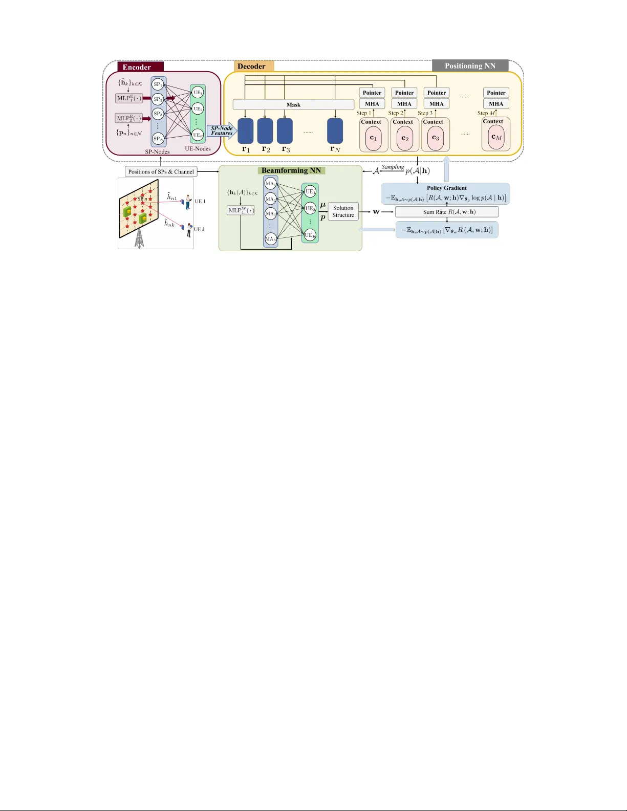
Learning to Jointly Optimize Antenna Positioning and Beamforming for Mo v able Antenna-Aided Systems Y ikun W ang ∗ † , Y ang Li † , Zeyi Ren ∗ , Jingreng Lei ∗ † , Y ik-Chung W u ∗ , and Rui Zhang ‡ ∗ Department of Electrical and Electronic Engineering, The University of Hong Kong, Hong Kong † School of Computing and Information T echnology , Great Bay Uni versity , Dongguan, China ‡ Department of Electrical and Computer Engineering, National University of Singapore, Singapore Emails: { ykwang, renzeyi, leijr , ycwu } @eee.hku.hk, liyang@gbu.edu.cn, elezhang@nus.edu.sg Abstract —The recently emerged movable antenna (MA) and fluid antenna technologies offer promising solutions to enhance the spatial degrees of freedom in wireless systems by dynamically adjusting the positions of transmit or recei ve antennas within given regions. In this paper , we aim to address the joint optimization problem of antenna positioning and beamforming in MA-aided multi-user downlink transmission systems. This problem inv olves mixed discrete antenna position and continuous beamforming weight variables, along with coupled distance con- straints on antenna positions, which pose significant challenges for optimization algorithm design. T o overcome these challenges, we propose an end-to-end deep learning framework, consisting of a positioning model that handles the discrete variables and the coupled constraints, and a beamforming model that handles the continuous variables. Simulation results demonstrate that the proposed framework achieves superior sum rate performance, yet with much reduced computation time compared to existing methods. Index T erms —Antenna positioning, combinatorial optimiza- tion, encoder-decoder model, graph neural networks, movable antenna. I . I N T R O D U C T I O N Mov able antenna (MA) [1] and fluid antenna (F A) [2] tech- nologies have garnered significant attention in recent years. Unlike traditional fixed-position antennas, MAs and F As can dynamically change their positions within a designated area. This flexibility allows antennas to move away from deep- fading positions, thereby improving the channel state and creating more fav orable conditions for wireless transmissions. The MA-aided system achiev es its optimum performance through antenna positioning [3]. Prior research has explored the antenna positioning problem in continuous space [3]–[6]. They aim to maximize v arious utility functions, e.g., sum rate, minimum signal-to-interference-plus-noise ratio (SINR), The work of Y ikun W ang, Y ang Li, and Jingreng Lei was supported in part by the National Natural Science Foundation of China (NSFC) under Grant 62571086, in part by Guangdong Basic and Applied Basic Research Foundation under Grant 2025A1515011658, and in part by Guangdong Research T eam for Communication and Sensing Integrated with Intelligent Computing (Project No. 2024KCXTD047). The codes for generating the simulation results in this paper are av ailable at: https://github .com/Y ikunW ang-EEE/RL-MA-joint-APS-and-BF . by optimizing the MA positions within a continuous des- ignated area. Additionally , some studies ha ve focused on the discrete antenna positioning problem [7]–[10], where the designated area is sampled into multiple position points. As such, the original positioning optimization in continuous space is transformed to a sampling point (SP) selection problem. This approach simplifies the hardware implementation b ut brings additional challenges for optimization algorithm design: the problem becomes combinatorial, and constrained by the coupled distance requirements between antennas. In [7], [8], graph theory-based approaches were proposed by modeling the problem as a fixed-hop shortest path problem. Howe ver , they are only applicable for the single-user scenario, limiting their applicability in multi-user systems when inter -user interference exists. While [9] proposed a generalized Bender’ s decom- position method to find the optimal antenna positions and beamformers that minimize the transmit power while ensuring the minimum SINR, this method suffers from exponential complexity in the worst case, which is practically hard for real-time implementation. Moreover , discrete antenna position and rotation joint design has been studied in six-dimensional mov able antenna (6DMA) aided systems [10]. Deep learning (DL) has been successfully applied to solve numerous optimization problems in communication systems, owing to its capacity to model complex functions and its af fordable real-time deployment compared to iterati ve- optimization algorithms. Howe ver , the joint design of discrete positioning and beamforming poses distincti ve challenges. First, the underlying optimization problem encompasses mixed discrete and continuous variables, where the discrete variables induce zero-gradient issues during backpropagation, rendering them difficult to handle within neural network (NN) architec- tures. Furthermore, the NN is required to generate discrete po- sitioning solutions that satisfy the coupled distance constraints, yet ensuring consistent fulfillment of these constraints in the NN’ s outputs remains inherently challenging. T o fill this gap, we propose a nov el DL framework com- prising two distinct NN models that handle positioning and beamforming sequentially . The positioning NN incorporates a graph neural network (GNN)-and-attention-based encoder- decoder architecture, which outputs the joint distribution of the positioning solutions. Through a judicious mask design, the generated positioning solutions are guaranteed to satisfy the coupled distance constraints, without any post-processing. Then, a GNN-based beamforming NN is employed to optimize the beamformers, leveraging an optimal solution structure to simplify the mapping to be learned. Furthermore, we introduce an end-to-end training algorithm, where the positioning NN and the beamforming NN are jointly trained in an unsupervised manner . Simulation results demonstrate that the proposed DL framew ork achieves superior sum rate performance than all baselines, while exhibiting significantly faster inference speed. I I . S Y S T E M M O D E L Consider an MA-aided downlink system with one base station (BS) serving K user equipments (UEs). The BS is equipped with M MAs and each UE is equipped with a single fixed-position antenna. The positions of the M MAs can be adjusted simultaneously within a predefined two-dimensional rectangular area, which is divided into N ≫ M SPs for placing the M MAs. The coordinate of the n -th SP is denoted by p n = [ x n , y n ] T , where x n and y n represent the coordinates along the x-axis and y-axis, respectiv ely , in the Cartesian coordinate system. Let ˜ h k ≜ [ ˜ h 1 k , ˜ h 2 k , . . . , ˜ h N k ] T denote the channel between the N SPs and UE k ∈ K ≜ { 1 , 2 , . . . , K } , which is assumed to be known [7]. Define the selected SP set as A ≜ { a 1 , a 2 , . . . , a M } , where a m ∈ N ≜ { 1 , 2 , . . . , N } . The receiv ed SINR of the k -th UE is given by SINR k =   h k ( A ) H w k   2 P K l =1 ,l  = k | h k ( A ) H w l | 2 + σ 2 k , (1) where h k ( A ) ∈ C M is the channel between the selected M SPs and the k -th UE, w k ∈ C M represents the trans- mit beamformer for the k -th UE, and σ 2 k is the power of the additiv e-white-Gaussian-noise. In this paper , we aim to maximize the sum rate by jointly optimizing A and w ≜ [ w T 1 , w T 2 , . . . , w T K ] T , which is formally formulated as max A , w R ( A , w ; h ) ≜ K X k =1 log 2 (1 + SINR k ) (2a) s.t. a m ∈ N , ∀ m ∈ M ≜ { 1 , 2 , . . . , M } , (2b) ∥ p a m − p a m ′ ∥ ≥ d min , ∀ m, m ′ ∈ M , m  = m ′ , (2c) K X k =1 ∥ w k ∥ 2 ≤ P max , (2d) where h ≜ [ ˜ h T 1 , ˜ h T 2 , . . . , ˜ h T K , p T 1 , p T 2 , . . . , p T N ] T denotes the known system parameters, d min is the minimum distance between two MAs, and P max is the maximum transmit power of the BS. Problem (2) is combinatorial, making it NP-hard to find the optimal solution. Furthermore, dev eloping a DL-based approach poses two key challenges: (a) the coupling between discrete and continuous variables; and (b) the highly non- con vex discrete constraints in (2c). In the subsequent section, we introduce a novel end-to-end DL framew ork that addresses these issues by handling the variables A and w sequentially through two distinct NN models. I I I . P R O P O S E D D L F R A M E W O R K The proposed end-to-end DL framework comprises two NN models: a positioning NN and a beamforming NN. Specifi- cally , the positioning NN takes the system parameter h as the input, and outputs the selected SP set A , i.e., A = F p ( h ) . Then, the beamforming NN takes A and h as the input, and outputs the beamformer w , i.e., w = F w ( A , h ) . These models are cascaded and trained jointly to pro vide near - optimal solutions while satisfying the constraints at the same time. W e then detail the design of F p ( · ) , F w ( · , · ) , and the joint training algorithm, respectiv ely . A. Design of F p ( · ) Since A consists of discrete variables, to avoid the zero- gradient due to a hard decision, we treat the elements in A as random variables, and striv e to learn the conditional probabil- ity of A giv en any h . Furthermore, due to the coupled distance constraints in (2c), each element of A depends on each other . Consequently , we factorize this conditional probability as p ( A | h ) = M Y t =1 p ( a m ( t ) | A t − 1 , h ) , (3) where a m ( t ) denotes the selected SP at the t -th step, A t − 1 ≜ { a m ( t ′ ) } t − 1 t ′ =1 represents all the SPs that hav e already been selected up to the ( t − 1 )-th step, and A 0 ≜ ∅ . Next, we construct an encoder-decoder model to learn the conditional probability (3), which also guarantees the coupled distance constraints in (2c). 1) Design of the encoder: The encoder G E ( · ) aims to build the mapping function from the system parameter h to the embeddings of all SPs denoted as R ≜ [ r 1 , r 2 , . . . , r N ] ∈ R n emb × N , capturing their suitability of antenna positioning, where n emb denotes the embedding dimension. T o this end, we model the MA-aided system as a graph, which includes two types of nodes, i.e., K UE-nodes and N SP-nodes, and there exists an edge between each UE-node and each SP-node. W e first show a desired permutation inv ariance (PI)-permutation equiv ariance (PE) property of G E ( · ) in the following property . Pr operty 1 (PI-PE Property of G E ( · ) ): Let ˆ h nk ≜ ˜ h π 2 ( n ) π 1 ( k ) , ˆ p n = p π 2 ( n ) , where π 1 ( · ) and π 2 ( · ) are permu- tations of the indices in K and N , respectiv ely . The mapping function G E ( · ) satisfies ˆ R = G E ( ℜ{ ˆ h } , ℑ{ ˆ h } ) , ∀ π 1 ( · ) : K → K , ∀ π 2 ( · ) : N → N , (4) if and only if R = G E ( ℜ{ h } , ℑ{ h } ) holds, where ˆ h ≜ [ ˆ h T π 1 (1) , ˆ h T π 1 (2) , . . . , ˆ h T π 1 ( K ) , p T π 2 (1) , p T π 2 (2) , . . . , p T π 2 ( N ) ] T , ˆ h k ≜ [ h π 2 (1) k , h π 2 (2) k , . . . , h π 2 ( N ) k ] T , and ˆ R ≜ [ r π 2 (1) , r π 2 (2) , . . . , r π 2 ( N ) ] . T o ensure Pr operty 1 , we design an edge-node GNN (EN- GNN) [11] as the foundation architecture of G E ( · ) , where the k -th UE-node feature and n -th SP-node feature of the l E -th hidden layer are expressed as f [ l E ] UE ,k and f [ l E ] SP ,n , and the corresponding edge feature is represented by e [ l E ] nk . The edge features and SP-node features are initialized as e [0] nk = MLP E 1  ℜ{ ˜ h nk } , ℑ{ ˜ h nk }  , ∀ k ∈ K , n ∈ N , (5a) f [0] SP ,n = MLP E 2 ( p n ) , ∀ n ∈ N , (5b) where MLP E 1 ( · ) and MLP E 2 ( · ) are 2 multi-layer perceptrons (MLPs), and the UE-node features { f [0] UE ,k } k ∈K are initialized as zero. After that, the encoder updates its node and edge features by a node-edge update mechanism, which is expressed as f [ l E ] UE ,k = MLP [ l E ] 2 f [ l E − 1] UE ,k , 1 N N X n =1 MLP [ l E ] 1  f [ l E − 1] SP ,n , e [ l E − 1] nk  ! , ∀ k ∈ K , (6) f [ l E ] SP ,n = MLP [ l E ] 4 f [ l E − 1] SP ,n , 1 K K X k =1 MLP [ l E ] 3  f [ l E − 1] UE ,k , e [ l E − 1] nk  ! , ∀ n ∈ N , (7) e [ l E ] nk = MLP [ l E ] 7 e [ l E − 1] nk , 1 N N X n ′ =1 MLP [ l E ] 5  e [ l E − 1] n ′ k , f [ l E − 1] UE ,k  , 1 K K X k ′ =1 MLP [ l E ] 6  e [ l E − 1] nk ′ , f [ l E − 1] SP ,n  ! , ∀ k ∈ K , n ∈ N , (8) where MLP [ l E ] 1 ( · ) - MLP [ l E ] 7 ( · ) are 7 MLPs. After L E layers’ update, the final SP-node feature f [ L E ] SP ,n serves as the required embedding r n . 2) Design of the decoder: The decoder obtains the condi- tional probability p ( A | h ) in M steps. At the t -th step, the decoder firstly extracts the current system state information, i.e., A t − 1 and h , by a conte xt embedding . Then, the multi-head attention (MHA) is applied between the context vector and R , to further extract deeper-le vel features. Finally , a P ointer [12] module is applied to capture the compatibilities between the context vector and R , so as to output the conditional probability p ( a m ( t ) |A t − 1 , h ) . The next SP a m ( t ) is sampled from this conditional probability . The aforementioned step is repeated for M times, until A is fully determined. The decoding process is illustrated in Fig. 1, where the detailed steps are presented as follows. Context Embedding: When t ≥ 2 , the context embedding is computed as c t = MLP X 1 1 t − 1 t − 1 X t ′ =1 MLP X 4 ( r a m ( t ′ ) ) , 1 N N X n =1 MLP X 2 p n , 1 K K X k =1 MLP X 3  ℜ{ ˜ h nk } , ℑ{ ˜ h nk }  !! , (9) Fig. 1. The illustration of the decoding process. where c t is a d h -dimensional vector , and MLP X 1 ( · , · ) -MLP X 4 ( · ) are 4 MLPs. When t = 1 , as A t − 1 = ∅ , we use a trainable parameter r ∗ ∈ R d h to replace the first input term of MLP X 1 ( · , · ) . MHA: For ease of expression, the index t is omitted. Let N h denote the number of attention heads. The query q [ h ] , the key k [ h ] n , and the value v [ h ] n at the h -th head are computed as follows: q [ h ] = W [ h ] Q c , ∀ h = 1 , 2 , . . . , N h , (10a) k [ h ] n = W [ h ] K r n , ∀ n ∈ N , ∀ h = 1 , 2 , . . . , N h , (10b) v [ h ] n = W [ h ] V r n , ∀ n ∈ N , ∀ h = 1 , 2 , . . . , N h , (10c) where q [ h ] , k [ h ] n , and v [ h ] n are all d v -dimensional vectors, d v = d h /N h , and W [ h ] Q , W [ h ] K , and W [ h ] V are trainable matrices. After that, we compute the relev ance scores be- tween the query and all ke ys. For each decoding step t , we define an av ailable SP set as ¯ N ≜ n n ∈ N       p n − p a m ( t ′ )    ≥ d min , ∀ t ′ < t o . As such, the rele- vance score with respect to the n -th SP is obtained as u [ n h ] n =    ( q [ n h ] ) T k [ n h ] n √ d v , if n ∈ ¯ N , −∞ , otherwise , (11) where we mask the SPs that have already been chosen or violate the distance constraint (2c) by setting their score as minus infinity . Consequently , we update the context vector by aggregating the v alue of each SP with the normalized rele v ance score serving as the corresponding weight: ˆ c = N h X h =1 " W [ h ] O N X n =1 e u [ h ] n P N n ′ =1 e u [ h ] n ′ v [ h ] n !# , (12) where the trainable matrix W [ h ] O ∈ R d h × d v maps the multiple aspects generated by MHA back to a unified space. Pointer: In the P ointer module, we first adopt a single-head attention mechanism to compute the compatibilities between the updated context vector ˆ c and all the SPs as u n = ( C · tanh  q T k n √ d h  , if n ∈ ¯ N , −∞ , otherwise , (13) where q = W Q ˆ c and k n = W K r n with trainable matrices W Q ∈ R d h × d h and W K ∈ R d h × d h , and the compatibili- ties are clipped within [ − C , C ] with a hyper-parameter C . Again, we use minus infinity to mask the SPs that have been already selected or violate the distance constraints. Finally , the conditional probability is obtained by normalizing the compatibilities as p ( a m ( t ) = n | A t − 1 , h ) = e u n P N n ′ =1 e u n ′ , ∀ n ∈ N . (14) Correspondingly , a m ( t ) is sampled from (14) during the train- ing process to enhance exploration. B. Design of F w ( · , · ) W e first exploit the optimal solution structure [13]: w k = √ p k  I M + K P i =1 µ i σ 2 k h i ( A ) h i ( A ) H  − 1 h k ( A )       I M + K P i =1 µ i σ 2 k h i ( A ) h i ( A ) H  − 1 h k ( A )      , ∀ k ∈ K , (15) where µ ≜ [ µ 1 , µ 2 , . . . , µ K ] T ∈ R K + and p ≜ [ p 1 , p 2 , . . . , p K ] T ∈ R K + are unknown parameters and should satisfy P K k =1 µ k = P K k =1 p k = P max such that (2d) can be satisfied. Exploiting this solution structure can simplify the mapping to be learned by the NN, by decreasing the number of unknown parameters from 2 K M to 2 K . The remaining task is to predict these lo w-dimensional parameters. For this purpose, we adopt the ENGNN, which consists of two types of nodes, i.e., M MA-nodes and K UE- nodes, and there exists an edge between each MA-node and each UE-node. The edge features are initialized as ˆ e [0] mk = MLP W 1 ( ℜ{ [ h k ( A )] m } , ℑ{ [ h k ( A )] m } ) , ∀ k ∈ K , m ∈ M , (16) and the node features { ˆ f [0] MA ,m } m ∈M and { ˆ f [0] UE ,k } k ∈K are initialized as zero. Similar to (6)-(8), after L W layers’ update, we obtain µ and p by [ µ k , p k ] T = FC ( ˆ f [ L W ] UE ,k ) , ∀ k ∈ K , (17a) µ ← P max · softmax ( µ ) , (17b) p ← P max · softmax ( p ) , (17c) where FC ( · ) is a fully-connected layer , and the softmax activ ation is employed to normalize µ and p . Finally , µ and p are substituted to (15) to get w . C. Joint T raining of F p ( · ) and F w ( · , · ) Based on the probabilistic modeling of p ( A| h ) in F p ( · ) , the joint training problem can be formulated as max θ p , θ w J ( θ p , θ w ) = E h , A∼ p ( A| h ) [ R ( A , w ; h )] , (18) where θ p and θ w denote the trainable parameters of F p ( · ) and F w ( · , · ) , respectiv ely , and the original constraints in (2b)-(2d) Algorithm 1 Joint Training of F p ( · ) and F w ( · , · ) 1: Input number of epochs N e , steps per epoch N s , and batch size B 2: Initialize θ p and θ w 3: for epoch = 1 , 2 , . . . , N e do 4: for step = 1 , 2 , . . . , N s do 5: Select a batch of input { h } from the training dataset 6: Output p ( A| h ) , A , and w corresponding to each training sample h 7: θ w ← Adam ( θ w , −∇ θ w J ( θ p , θ w )) 8: θ p ← Adam ( θ p , −∇ θ p J ( θ p , θ w )) 9: end for 10: end for are satisfied through the design of F p ( · ) and F w ( · , · ) . Next, we show how to update θ p and θ w . 1) Update of θ p : Since A is sampled according to p ( A| h ) , R ( A , w ; h ) is non-differentiable with respect to θ p . Howe ver , since p ( A| h ) itself is differentiable with respect to θ p , we can calculate the gradient of J ( θ p , θ w ) with respect to θ p using the P olicy-Gradient strategy [14]: ∇ θ p J ( θ p , θ w ) = E h   X A∼ p ( A| h ) R ( A , w ; h ) ∇ θ p p ( A | h )   = E h   X A∼ p ( A| h ) R ( A , w ; h ) p ( A| h ) ∇ θ p log p ( A | h )   = E h , A∼ p ( A| h )  R ( A , w ; h ) ∇ θ p log p ( A | h )  . (19) Then, θ p is updated to maximize (18) by a mini-batch stochas- tic gradient ascent algorithm, which can be implemented with the Adam optimizer [15]. 2) Update of θ w : Since R ( A , w ; h ) is differentiable with respect to w and consequently with respect to θ w , we can compute the gradient of J ( θ p , θ w ) with respect to θ w by ∇ θ w J ( θ p , θ w ) = E h , A∼ p ( A| h ) [ ∇ θ w R ( A , w ; h )] . (20) Consequently , θ w is updated to maximize (18) by a mini-batch stochastic gradient ascent algorithm using the Adam optimizer . The joint training algorithm is summarized in Algorithm 1, where the negati ve gradient is adopted in lines 7 and 8 to set a gradient ascent update in the Adam optimizer . After training, F p ( · ) and F w ( · , · ) with parameters θ p and θ w are used to predict A and w giv en any h . The proposed overall DL framework is summarized in Fig. 2. I V . N U M E R I C A L R E S U LT S In this section, we ev aluate the performance of the proposed DL framew ork via numerical results. W e consider an MA- aided system where the BS is equipped with [4 , 9] MAs to serve 4 single-antenna UEs. The size of the 2D rectangular transmit area is 2 λ × 2 λ , where each side is uniformly sampled with [5 , 8] points, resulting in { 25 , 36 , 49 , 64 } SPs, and the wa velength λ = 60 mm. The minimum distance between Fig. 2. Structure of our proposed DL framework. ev ery two MAs is set as d min = 30 mm. The distance between the k -th UE and the BS, denoted as D k , is uniformly distributed within [100 , 200] in meters. The noise power is set as − 100 dBm. W e consider the field-response channel model (see (3)-(6) in [1]) where { ˜ h k } k ∈K is determined by the positions of SPs, the path-response matrix Σ k ≜ diag n [ η 1 k , η 2 k , . . . , η L r k ] T o , the elev ation angle of departure (AoD) { θ k,l t } K,L t k =1 ,l t =1 , and the azimuth AoD { ϕ k,l t } K,L t k =1 ,l t =1 , where L t = L r = 16 are the numbers of transmit paths and recei ve paths, re- spectiv ely , and η l r k follows complex Gaussian distribution C N  0 , L 0 D − α k  with L 0 = 34 . 5 dB and α = 3 . 67 . Besides, the probability density function of AoDs is f AoD ( θ k,l t , ϕ k,l t ) = cos θ k,l t / 2 π , θ k,l t ∈ [ − π / 2 , π/ 2] , ϕ k,l t ∈ [ − π / 2 , π/ 2] . For the proposed NN model, all the MLPs are implemented by 2 linear layers, each followed by a ReLU activ ation function. The encoder of F p ( · ) has L E = 3 layers, with n emb = 128 and d h = 256 . The number of heads in the MHA model is N h = 8 . The clipping logit is set to C = 8 . Moreov er , F w ( · , · ) has L W = 3 hidden layers, each with a hidden dimension of 64. In the training procedure, the number of epochs is set to 100, where each epoch consists of 50 mini- batches with a batch size of 1024 . A learning rate 10 − 4 is adopted to update the trainable parameters θ p and θ w through Algorithm 1 using the Adam optimizer . After training, we test the performance of the proposed DL framew ork on a testing set comprising 1000 samples. The implementation of the experiment is under the PyT orch version 2.1.2+cu12, operating on an NVIDIA GeForce GTX 4090 GPU. W e consider four baselines for comparison: W e assume that the ele vation AoD { θ k,l t } K,L t k =1 ,l t =1 , azimuth AoD { ϕ k,l t } K,L t k =1 ,l t =1 , and the path response coefficients { η l r k } K,L r k =1 ,l r =1 are perfectly estimated [16], enabling the perfect recovery of the channel h . • Random+WMMSE: This method in volv es randomly se- lecting M elements from N to construct A . If A violates the constraints in (2c), the selection is repeated until the constraints are satisfied. Subsequently , with the MA positions determined, w is computed using the WMMSE algorithm [17]. • Str ongest+WMMSE: For this approach, the average channel gain of each SP with respect to all K UEs is first calculated and treated as the equiv alent channel gain for that SP . The SPs exhibiting the strongest channel gains are then selected iteratively over M steps, with SPs violating (2c) masked in each step. Follo wing the positioning, w is obtained via the WMMSE algorithm. • Str ongest+ZF: This method combines strongest-channel- based positioning with the zero-forcing beamforming [18]. • FP-C: W e modify an approach that jointly optimizes continuous antenna positioning and beamforming for MA-aided systems [6]. T o obtain discrete antenna posi- tions that satisfy the discrete constraints in (2c), in each iteration of FP-C we project the position of each MA to its nearest discrete SP that satisfies (2c) sequentially . W e first compare the sum rate performance under different power budgets. In Fig. 3, with M = 6 and N = 49 , it can be observed that Random+WMMSE and Str ongest+ZF perform badly due to their heuristic antenna positioning and beamforming strategies, respectively . Moreover , the proposed DL framework outperforms all baselines particularly at higher transmit power . This demonstrates the great capability of the proposed framew ork in mitigating interference, particularly when inter-user interference becomes stronger . Next, we compare the average computation time across various approaches. It can be observed from T able I that the computation time of the proposed DL framework is substan- tially shorter than the iterative optimization-based methods, including WMMSE and FP-C . Fig. 3. The sum rate performance comparison under different power budgets when M = 6 and N = 49 . T ABLE I C O MPA R IS O N O F A V E RA G E C OM P U T ATI O N T I M E Method T ime (ms) Strongest+ZF 3.26 Random+WMMSE 644.37 Strongest+WMMSE 644.66 FP-C 3682.82 Proposed 7.89 (a) Under different M ’s. (b) Under different N ’s. Fig. 4. The sum rate performance of our proposed DL framework under different M ’s and N ’ s. Finally , we ev aluate the performance of the proposed DL framew ork across a range of system settings. W e first set P max = 20 dBm and N = 49 , and plot the sum rate against M in Fig. 4(a). As observed, the proposed DL framework achiev es highest sum rates across different values of M . Next, in Fig. 4(b), we plot the sum rate against N when P max = 20 dBm and M = 6 . As observed from Fig. 4(b), the proposed DL framew ork achieves superior performance across different values of N . In contrast to heuristic positioning methods such as Strong est and Random which perform poorly , our proposed method achieves the best performance no matter when the number of SPs is limited, or when the number of SPs is sufficient but with more challenging constraints. V . C O N C L U S I O N In this paper, we have proposed a nov el DL frame work for solving the discrete antenna positioning and beamforming design problem in MA-aided multi-user systems. First, an encoder-decoder -based positioning NN has been de veloped to determine the MA positions, incorporating a sequential decoding strategy with a mask design to handle the discrete variables and the coupled distance constraints. Subsequently , the continuous variables are optimized using a beamforming NN, which lev erages an ENGNN model informed by an optimal solution structure. Furthermore, we have introduced a joint training algorithm to jointly optimize the positioning NN and the beamforming NN. Numerical results hav e shown that the proposed end-to-end DL framew ork outperforms baseline approaches with much faster computation speed. R E F E R E N C E S [1] L. Zhu, W . Ma, and R. Zhang, “Modeling and performance analysis for movable antenna enabled wireless communications, ” IEEE T rans. on W ireless Commun. , vol. 23, no. 6, pp. 6234–6250, 2024. [2] K.-K. W ong, A. Shojaeifard, K.-F . T ong, and Y . Zhang, “Fluid antenna systems, ” IEEE T rans. on Wir eless Commun. , vol. 20, no. 3, pp. 1950– 1962, 2021. [3] W . Ma, L. Zhu, and R. Zhang, “MIMO capacity characterization for mov able antenna systems, ” IEEE Tr ans. on W ir eless Commun. , vol. 23, no. 4, pp. 3392–3407, 2024. [4] L. Zhu, W . Ma, B. Ning, and R. Zhang, “Movable-antenna enhanced multiuser communication via antenna position optimization, ” IEEE T rans. on W ir eless Commun. , vol. 23, no. 7, pp. 7214–7229, 2024. [5] Y . Jin, Q. Lin, Y . Li, and Y .-C. W u, “Handling distance constraint in mov able antenna aided systems: A general optimization framew ork, ” in IEEE Int. W orkshop Signal Pr ocess. Advances W ireless Commun. (SP A WC) , 2024. [6] Z. Cheng, N. Li, J. Zhu, X. She, C. Ouyang, and P . Chen, “Sum- rate maximization for fluid antenna enabled multiuser communications, ” IEEE Commun. Letters , vol. 28, no. 5, pp. 1206–1210, 2024. [7] W . Mei, X. W ei, B. Ning, Z. Chen, and R. Zhang, “Movable-antenna po- sition optimization: A graph-based approach, ” IEEE Wir eless Commun. Letters , vol. 13, no. 7, pp. 1853–1857, 2024. [8] W . Mei, X. W ei, Y . Liu, B. Ning, and Z. Chen, “Movable-antenna position optimization for physical-layer security via discrete sampling, ” in IEEE Globe Commun. Conf. (GLOBECOM) , 2024. [9] Y . Wu, D. Xu, D. W . K. Ng, W . Gerstacker , and R. Schober, “Mov able antenna-enhanced multiuser communication: Jointly optimal discrete antenna positioning and beamforming, ” in IEEE Globe Commun. Conf. (GLOBECOM) , 2023. [10] X. Shao, R. Zhang, Q. Jiang, and R. Schober, “6D movable antenna en- hanced wireless network via discrete position and rotation optimization, ” IEEE J. Sel. Areas Commun. , vol. 43, no. 3, pp. 674–687, 2025. [11] Y . W ang, Y . Li, Q. Shi, and Y .-C. Wu, “ENGNN: A general edge- update empowered GNN architecture for radio resource management in wireless networks, ” IEEE T rans. on W ir eless Commun. , vol. 23, no. 6, pp. 5330–5344, 2024. [12] I. Bello, H. Pham, Q. V . Le, M. Norouzi, and S. Bengio, “Neural combinatorial optimization with reinforcement learning, ” in Int. Conf. on Learn. Repr esentations (ICLR) , 2017. [13] E. Bj ¨ ornson, M. Bengtsson, and B. Ottersten, “Optimal multiuser trans- mit beamforming: A difficult problem with a simple solution structure, ” IEEE Signal Pr ocess. Mag. , vol. 31, no. 4, pp. 142–148, 2014. [14] R. W illiams, “Simple statistical gradient-following algorithms for con- nectionist reinforcement learning, ” Mach. Learn. , 1992. [15] D. P . Kingma and J. Ba, “ Adam: A method for stochastic optimization, ” arXiv:1412.6980 , 2014. [16] W . Ma, L. Zhu, and R. Zhang, “Compressed sensing based channel esti- mation for movable antenna communications, ” IEEE Commun. Letters , vol. 27, no. 10, pp. 2747–2751, 2023. [17] S. S. Christensen, R. Agarwal, E. De Carvalho, and J. M. Ciof fi, “W eighted sum-rate maximization using weighted MMSE for MIMO- BC beamforming design, ” IEEE T rans. on W ireless Commun. , vol. 7, no. 12, pp. 4792–4799, 2008. [18] Q. Spencer, A. Swindlehurst, and M. Haardt, “Zero-forcing methods for downlink spatial multiplexing in multiuser mimo channels, ” IEEE T rans. on Signal Pr ocess. , vol. 52, no. 2, pp. 461–471, 2004.