Near-Optimal Constrained Feedback Control of Nonlinear Systems via Approximate HJB and Control Barrier Functions

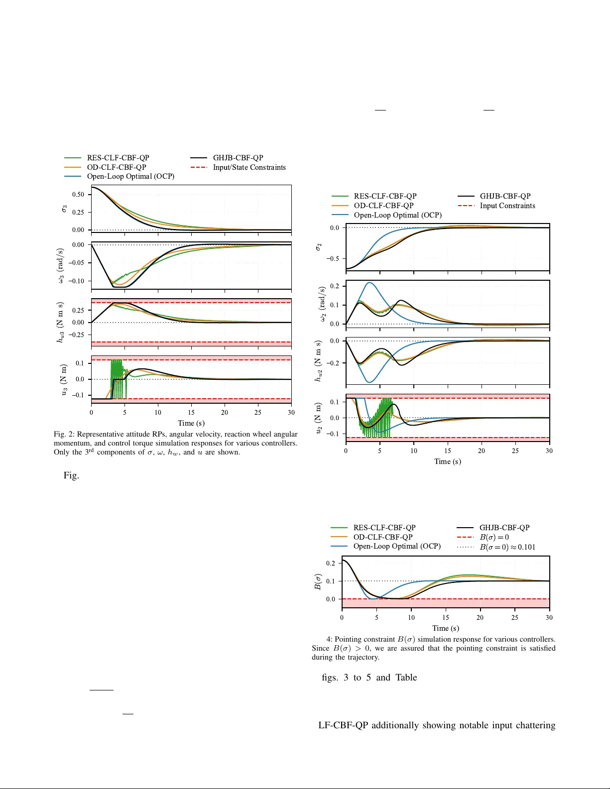
Near -Optimal Constrained F eedback Control of Nonlinear Systems via A pproximate HJB and Contr ol Barrier Functions Milad Alipour Shahraki and Laurent Lessard Abstract — This paper presents a two-stage framew ork for constrained near -optimal feedback control of input-affine non- linear systems. An approximate v alue function for the un- constrained contr ol problem is computed offline by solving the Hamilton–Jacobi–Bellman equation. Online, a quadratic program is solved that minimizes the associated approximate Hamiltonian subject to safety constraints imposed via control barrier functions. Our proposed architecture decouples per- formance fr om constraint enf orcement, allowing constraints to be modified online without recomputing the value function. V alidation on a linear 2-state 1D hovercraft and a nonlinear 9-state spacecraft attitude control problem demonstrates near - optimal performance r elative to open-loop optimal control benchmarks and superior performance compared to control L yapunov function-based controllers. I . I N T R O D U C T I O N The optimal feedback control problem for general nonlin- ear systems remains a central challenge in control theory . The Hamilton–Jacobi–Bellman (HJB) equation provides the theoretical foundation for optimal control; howe ver , its non- linear partial dif ferential equation (PDE) structure renders analytical solutions generally unavailable, while the curse of dimensionality makes numerical solutions intractable for high-dimensional systems [1]. In practice, control systems must also satisfy safety-critical constraints, such as actuator limits, state bounds, and geometric exclusion zones, further complicating the design of optimal controllers. Model predicti ve control (MPC) addresses both optimality and safety via receding-horizon optimization, b ut solving a nonlinear program online limits real-time applicability for fast or high-dimensional systems. Alternativ ely , one can address optimality and safety sep- arately . On the optimization side, approximate dynamic programming methods solve relaxed forms of the HJB equation: the Successiv e Galerkin Approximation (SGA) [2] projects the Generalized HJB (GHJB) PDE onto polynomial bases, while Sum-of-Squares (SOS) programming [3], [4] re- places intractable non-neg ativity conditions with semidefinite constraints. Policy iteration schemes [5], [6] then produce monotonically impro ving v alue function approximations with global stability guarantees. Ho wev er, these methods typically address unconstrained problems; embedding constraints into these methods is nontri vial, as it can significantly increase the M. Alipour Shahraki is with the Department of Electrical and Com- puter Engineering, Northeastern University , Boston, MA 02115, USA alipourshahraki.m@northeastern.edu L. Lessard is with the Department of Mechanical and Indus- trial Engineering, Northeastern Univ ersity , Boston, MA 02115, USA l.lessard@northeastern.edu problem size, require higher-order approximation to maintain feasibility , or render the problem infeasible altogether . On the constraint enforcement side, Control Barrier Functions (CBFs) [7] and their high-order extensions (HOCBFs) [8] translate state constraints into linear inequali- ties on the control input, enabling real-time enforcement via quadratic programs (QPs). CBFs hav e been combined with Control L yapunov Functions (CLFs) in CLF-CBF-QP archi- tectures [9] for simultaneous stability and safety . Ho wev er, as observed in our prior work on spacecraft attitude control [10], CLF-based approaches hav e several limitations: (i) CLF-QP objectiv es guarantee stability b ut not optimality , and typically require hand-designed L yapunov functions via input-output linearization [10]; (ii) fixed decay rates cause input chattering at lo w sampling frequencies [10], [11]; and (iii) the pre- scribed decay rate introduces a comparison function design problem [12], where the choice of decay shape governs a feasibility/con ver gence trade-of f further complicated by actuator bounds. All three issues stem from enforcing a pointwise decay rate and require nontrivial design choices. Sev eral recent works couple safety and performance by incorporating CBF conditions directly into the value function computation [13]–[15], but some guarantee only ultimate boundedness rather than asymptotic stability [13], and all require a full problem re-solve if the safe set changes, eliminating the flexibility to modify constraints online. This work bridges the gap between the two described lines of work. In contrast to [13]–[15], we propose a two-stage architecture that decouples performance optimization from safety constraint enforcement. The ke y idea is to replace the hand-designed CLF with a near-optimal value function computed offline via policy iteration, and to enforce con- straints online through a CBF-QP that requires only the value function gradient and is agnostic to ho w it was obtained. The contributions of this paper are as follo ws: 1. W e propose the GHJB-CBF-QP , a con vex QP that uses the gradient of a precomputed value function to driv e the system toward near -optimal trajectories, while CBF constraints enforce state safety and input bounds. Unlike CLF-CBF-QP [9], [10], the objectiv e reflects optimality rather than mere stability , and the controller is inherently chatter-free: it a voids input-output linearization entirely and imposes no CLF decay rate constraint, eliminating all three CLF limitations discussed above. 2. W e characterize the optimality gap, decomposing it into three terms: value function approximation error , constraint projection error, and CBF conservatism, each admitting a separate mitigation strate gy , and sho w that the CBF conservatism term v anishes for integrator-state constraints (relativ e degree one with zero drift). 3. W e validate the frame work on a 1D hovercraft (linear, 2 states) and a spacecraft attitude control problem (non- linear , 9 states), demonstrating near-optimal performance relativ e to open-loop optimal control and superior perfor- mance compared to CLF-CBF-QP controllers with real- time implementability and formal safety guarantees. The remainder of this paper is organized as follo ws. Section II formulates the problem and presents the offline value function approximation via polic y iteration. Section III dev elops the online GHJB-CBF-QP controller , including its optimality and safety properties. Section IV validates the framew ork on linear and nonlinear examples, and Section V concludes with future research directions. I I . P R O B L E M F O R M U L A T I O N A. System Dynamics and Objectives Consider a nonlinear input-affine control system ˙ x = f ( x ) + g ( x ) u, x (0) = x 0 , (1) where x ( t ) ∈ R n is the state, u ( t ) ∈ R m is the control input, and f : R n → R n , g : R n → R n × m are assumed to be locally Lipschitz continuous with f (0) = 0 . The system is subject to state constraints h i ( x ) ≤ 0 , i = 1 , . . . , n h and input constraints u ∈ U : = { u | u min ≤ u ≤ u max } . W e aim to minimize the infinite-horizon cost J ( x 0 , u ( · )) = Z ∞ 0  q ( x ) + u T R u  d t s.t. (1) , (2) where q : R n → R ≥ 0 is positi ve semidefinite with q (0) = 0 (here we consider q ( x ) : = x T Qx with Q ⪰ 0 ), and R ≻ 0 , while satisfying input and state constraints. Our approach decouples this problem into two layers. First, the unconstrained optimal control problem is approxi- mately solved offline via the HJB equation. Then, constraints are enforced online via a CBF-QP . W e begin by revie wing the unconstrained problem. B. Hamilton–J acobi–Bellman (HJB) Equation Ignoring constraints for the moment, the optimal value function V ∗ ( x 0 ) = min u ( · ) J ( x 0 , u ( · )) satisfies the HJB equation H ( V ∗ ) = 0 , where the Hamiltonian is H ( V ) : = ∇ V T f ( x ) + q ( x ) − 1 4 ∇ V T g ( x ) R − 1 g ( x ) T ∇ V , (3) and the optimal feedback control is u ∗ ( x ) = − 1 2 R − 1 g ( x ) T ∇ V ∗ ( x ) . (4) Solving H ( V ∗ ) = 0 exactly is generally intractable since (3) is a nonlinear PDE due to the quadratic dependence on ∇ V . For a gi ven admissible policy u ( x ) , this nonlinearity is removed: the associated value function V satisfies the Generalized HJB (GHJB) equation, a linear PDE in ∇ V : ∇ V T  f ( x ) + g ( x ) u  + q ( x ) + u T Ru = 0 . (5) C. Relaxed HJB F ormulation Follo wing [5], we relax the HJB equality to an inequality . Let Ω ⊂ R n be a compact set containing the origin, and P denote the set of positiv e definite, proper , C 1 functions. The relaxed problem is: min V Z Ω V ( x ) d x s.t. H ( V ) ≤ 0 , V ∈ P . (6) Assumption 1: There exist V 0 ∈ P and a feedback policy u 0 such that L ( V 0 , u 0 ) ≥ 0 for all x ∈ R n , where L ( V , u ) : = −∇ V T ( f + g u ) − q ( x ) − u T Ru is the Bellman operator . Assumption 2: There exists V ∗ ∈ P satisfying the HJB equation H ( V ∗ ) = 0 . Theorem 1 (Relaxed Solution Properties [5]): Under the abov e assumptions: (i) Problem (6) has a nonempty fea- sible set. (ii) F or an y feasible V , the control ¯ u ( x ) = − 1 2 R − 1 g T ∇ V is globally asymptotically stabilizing. (iii) V upper-bounds the cost: V ( x 0 ) ≥ J ( x 0 , ¯ u ) for all x 0 . (iv) V ∗ ( x ) ≤ V ( x ) for all feasible V . (v) V ∗ is the global optimum of (6). Property (ii) is the ke y insight: any feasible V simultane- ously provides a stabilizing controller and a L yapunov certifi- cate, since ˙ V = H ( V ) − q ( x ) − ¯ u T R ¯ u ≤ − q ( x ) . Minimizing R V d x tightens this bound, dri ving V tow ard V ∗ . D. V alue Function Appr oximation Our proposed online control framew ork requires a pre- computed approximate value function ˆ V . The quality of ˆ V affects performance but not safety (Proposition 2). For our numerical examples, we used two different ap- proximation methods, which we now briefly re view . In all cases, we parameterized V as a polynomial ˆ V ( x ) = P i c i m i ( x ) in e ven-degree monomials and solved for the coefficients via policy iteration [5]: alternating be- tween e valuating the current policy (solving for V ( k ) with L ( V ( k ) , u ( k ) ) ≥ 0 ) and impro ving via u ( k +1) = − 1 2 R − 1 g T ∇ V ( k ) . Under Assumptions 1 and 2, the iterates { V ( k ) } decrease monotonically tow ard V ∗ , and each policy is globally stabilizing [5]. The policy ev aluation step requires verifying L ( V ( k ) , u ( k ) ) ≥ 0 . For our linear e xample, we used Successiv e Galerkin Approximation (SGA) [2], which re- duces the computation to solving a system of linear equations with analytically computable entries, con verging to the exact LQR solution as basis richness increases. For our second example, a nonlinear polynomial system, we used Sum-of- Squares (SOS) programming, which replaced the (NP-hard) non-negati vity check with a semidefinite program, inheriting the same con vergence guarantees [5]. E. Safety via Control Barrier Functions (CBFs) W e now revie w the (high-order) CBF tools used in the online layer . Definition 1 (Relative Degr ee [8]): A (sufficiently) dif- ferentiable function h : R n → R has relative degree r with respect to (1) if L g L k f h ( x ) = 0 for all k < r − 1 and L g L r − 1 f h ( x )  = 0 . Definition 2 (HOCBF [7], [8]): Given B ( x ) ≥ 0 with relativ e degree r and α 1 , . . . , α r > 0 , define ψ 0 ( x ) : = B ( x ) , ψ k ( x ) : = ˙ ψ k − 1 ( x ) + α k ψ k − 1 ( x ) , (7) for k = 1 , . . . , r , with C k = { x | ψ k ( x ) ≥ 0 } . Then B is a HOCBF if sup u ∈U ψ r ( x, u ) ≥ 0 for all x ∈ C 0 ∩ · · · ∩ C r − 1 . Theorem 2 (HOCBF F orwar d In variance [7], [8]): If B is a HOCBF and u ( x ) satisfies ψ r ( x, u ) ≥ 0 on C 0 ∩ · · · ∩ C r − 1 , then this set is forward in v ariant. For r = 1 , the HOCBF condition reduces to the standard CBF constraint [7]: L f B + L g B u ≥ − α 1 B , and for r = 2 , expanding (7) yields L 2 f B + L g L f B · u + ( α 1 + α 2 ) L f B + α 1 α 2 B ≥ 0 , which is af fine in u and directly incorporable into a QP . I I I . G H J B - C B F - Q P C O N T RO L L E R W e now present our main contribution, GHJB-CBF-QP , which combines the offline value function from Section II-D with the CBF machinery from Section II-E into a single QP . A. F ormulation Giv en the precomputed ˆ V ( x ) , the online QP objectiv e is deriv ed from the GHJB equation. Recall from (5) that the Hamiltonian e valuated at a control u (before minimization) is ∇ V ( x ) T ( f ( x ) + g ( x ) u ) + q ( x ) + u T R u . Since the drift terms ∇ V T f and q do not depend on u , minimizing over u is equi valent to minimizing J GHJB ( u ) = ∇ ˆ V ( x ) T g ( x ) u + u T R u, (8) which is con ve x quadratic in u . The unconstrained minimizer is u ∗ = − 1 2 R − 1 g T ∇ ˆ V , recov ering the offline polic y (4) with ˆ V in place of V ∗ . The GHJB-CBF-QP augments this objectiv e with CBFs/HOCBFs and input constraints: min u ∇ ˆ V ( x ) T g ( x ) u + u T R u s.t. ψ r ( x, u ) ≥ 0 , (CBFs/HOCBFs) u min ≤ u ≤ u max . (Input bounds) (9) By Theorem 2, any feasible solution guarantees forward in variance of all safe sets, regardless of ˆ V . Remark 1 (No comparison function): Unlike CLF-CBF- QPs, which require a decay constraint ˙ V ≤ − γ ( V ) with a carefully chosen comparison function γ [12] and a slack variable to ensure feasibility under actuator bounds, the GHJB-CBF-QP (9) imposes no decay rate constraint and requires no slack variable. The effecti ve decay is determined implicitly by ∇ ˆ V , eliminating both design choices. B. Theor etical Pr operties Proposition 1 (Optimality Recovery): In (9), if all con- straints are inacti ve, the solution recovers the unconstrained offline policy: u GHJB - CBF = − 1 2 R − 1 g T ∇ ˆ V . Pr oof: W ith no active constraints, (9) reduces to unconstrained minimization of (8). Setting ∂ J GHJB /∂ u = g T ∇ ˆ V + 2 Ru = 0 yields u ∗ = − 1 2 R − 1 g T ∇ ˆ V . Proposition 2 (Safety-P erformance Decoupling): For any value function approximation ˆ V , the online policy (9): (i) is guaranteed to be safe and (ii) recovers optimal performance as ˆ V → V ∗ when the constraints are inactive. Pr oof: (i) The CBF and HOCBF constraints in (9) are enforced as hard constraints regardless of the objectiv e. By Theorem 2, any feasible u renders the safe sets forward in variant, independent of ˆ V . (ii) As ˆ V → V ∗ , we have ∇ ˆ V → ∇ V ∗ , so the QP objecti ve approaches the true Hamil- tonian minimization. By Proposition 1, whenev er constraints are inactive the controller recovers u ∗ = − 1 2 R − 1 g T ∇ V ∗ . Remark 2 (Optimality Gap Decomposition): Let J c ( x 0 ) denote the cost achieved by the constrained optimal controller (solving (2) subject to all state and input constraints), and let J GHJB - CBF ( x 0 ) denote the cost achiev ed by the GHJB-CBF-QP controller (9). The total suboptimality J GHJB - CBF ( x 0 ) − J c ( x 0 ) can be attributed to three sources: (i) ∆ approx : error from approximating V ∗ with ˆ V ; (ii) ∆ pro j : error from projecting the unconstrained policy onto the feasible set, which is zero when constraints are inactive; and (iii) ∆ CBF : conservatism of the CBF formulation relati ve to hard state constraints, which depends on the constraint structure and the parameter α (CBF decay rate). These sources are conceptually distinct and admit separate mitigation strategies: ∆ approx by improving the value function approximation, ∆ pro j by loosening constraints, and ∆ CBF by increasing α or exploiting fa vorable constraint structure (see Proposition 3). T o our knowledge, the following observation has not been formally stated in prior work, though it follows directly from the CBF construction. Proposition 3 (Inte grator-State Constraints): Consider a box constraint x i, min ≤ x i ≤ x i, max on a state component whose dynamics satisfy ˙ x i = f i ( x ) + g i ( x ) T u with f i ( x ) = 0 for all x and t . Define ¯ B ( x ) = x i, max − x i and ¯ B ( x ) = x i − x i, min . Then each CBF has relativ e degree one with L f B = 0 , and the CBF constraints reco ver the hard state constraints exactly as α → ∞ , so ∆ CBF = 0 . Pr oof: Since f i ( x ) = 0 , the Lie deri vati ves are L f ¯ B = − f i = 0 and L g ¯ B = − g i ( x ) T , so the CBF conditions reduce to − g T i u ≥ − α ( x i, max − x i ) and g T i u ≥ − α ( x i − x i, min ) . In the interior ( x i, min < x i < x i, max ), the right-hand sides tend to −∞ as α → ∞ , so the constraints become vacuous and impose no restriction on u . At the boundary x i = x i, max , the upper constraint becomes g T i u ≤ 0 , which exactly prevents x i from increasing past the boundary (since ˙ x i = g T i u ). The lower boundary is analogous. Thus, in the limit α → ∞ , the CBF constraints are equi valent to the hard state constraints, and no conservatism is introduced. In practice, a moderately lar ge α (e.g., α = 10 ) suffices to make the CBF conservatism practically vanish, so that ∆ CBF ≈ 0 without requiring α → ∞ (see Section IV). I V . A P P L I C A T I O N E X A M P L E S W e v alidate the GHJB-CBF-QP on two examples: Exam- ple 1 on a linear system where the exact optimum is known, and Example 2 on a nonlinear system with constraints of relativ e degree one (Case 1) and two (Case 2). T ogether , the examples demonstrate (i) near-zero CBF conservatism for integrator-state constraints, (ii) the flexibility to handle different constraint types without modifying the offline value function, and (iii) the inherent suboptimality of pointwise QP-based controllers relati ve to trajectory-aware optimal control for higher-order constraints. All simulations run in Julia on an Apple M2 Pro chip with 32 GB of RAM at a sampling rate of 10 Hz. The constrained Optimal Control Problem (OCP) (2) is solved via direct transcription in JuMP/Ipopt; all QP-based controllers use JuMP/HiGHS. MPC and constrained Linear Quadratic Regulator (LQR) serve as additional benchmarks for Example 1. The Optimal-Decay (OD) and Rapidly- Exponentially-Stabilizing (RES) CLF-CBF-QP controllers for Example 2 are from [10]. All shared parameters are identical across controllers. A. Example 1 (Linear): 1D Hover craft The 1D hovercraft has state x = [ p, v ] T ∈ R 2 (position and velocity). The input u ∈ R is the thrust force. The system is a double integrator in input-affine form (1) with f ( x ) : =  v 0  , g ( x ) : =  0 1  . The SGA uses basis functions { p 2 , v 2 , pv } over Ω = [ − 1 , 1] 2 and the initial policy u 0 = − p − v . The SGA policy iteration took approximately 0 . 4 seconds and conv erged after 4 iterations. The velocity is constrained by v min ≤ v ≤ v max and the input by u min ≤ u ≤ u max . Since ˙ v = u , velocity is an integrator -state with relativ e degree one. Defining ¯ B ( x ) = v max − v and ¯ B ( x ) = v − v min , the CBF conditions (Proposition 3) reduce to − α ( v − v min ) ≤ u ≤ α ( v max − v ) . The parameters used in the simulations are x 0 = [10 , 0] T , Q = I 2 , R = 1 , α = 10 , | v | ≤ 1 m/s, and | u | ≤ 1 N. 0 5 10 p ( m ) 1 0 1 v ( m / s ) 0 5 10 15 20 25 30 T ime (s) 1 0 1 u ( N ) Constrained LQR MPC Open-Loop Optimal (OCP) GHJB-CBF-QP Input/State Constraints Fig. 1: Simulated trajectories (position, velocity , input) for the 1D hovercraft for various controllers. All trajectories are the same for this example. T ABLE I: Cost and wall clock time comparison for different controllers. For OCP , this is the offline computation time. For the other control methods, this is the total online computation time (all iterations). The corresponding state and input trajectories are shown in Fig. 1. Control Method Cost J T ime (s) Constrained LQR 398 . 3448 0 . 07 MPC 398 . 3475 1 . 07 Open-Loop Optimal (OCP) 398 . 3440 0 . 03 GHJB-CBF-QP 398 . 3448 0 . 28 The simulation results in Fig. 1 and T able I confirm that the closed-loop GHJB-CBF-QP achiev es near -identical performance (all trajectories are superimposed) to all three benchmarks for linear systems. All reported times reflect the total wall clock time to generate the full trajectory; for QP-based controllers this is the cumulative cost of all per - step solves, confirming real-time implementability . The close agreement with the open-loop OCP is consistent with Propo- sition 3, which predicts ∆ CBF ≈ 0 for the velocity constraint since it is an integrator-state with zero drift. Moreover , the relativ e-degree-one structure means the constraints reduce to instantaneous bounds on u , for which pointwise projection incurs little cost penalty ( ∆ pro j ≈ 0 ). B. Example 2 (Nonlinear): Spacecraft Attitude Contr ol W e apply the framew ork to spacecraft attitude control with reaction wheels, previously studied in [10] using CLF- CBF-QP . The state is x = [ σ T , ω T , h T w ] T ∈ R 9 , where σ ∈ R 3 denotes the Rodrigues Parameters (RPs) attitude representation, ω ∈ R 3 is the angular velocity in the body- fixed frame, and h w ∈ R 3 is the reaction wheel angular momentum. The input u ∈ R 3 is the control torque. Three identical, axially symmetric reaction wheels are assumed to be aligned with the spacecraft’ s principal axes. The system takes the input-affine form (1) with [10], [16] f ( x ) : =   G ( σ ) ω − J − 1 [ ω ] × ( J ω + h w ) 0 3 × 1   , g ( x ) : =   0 3 × 3 J − 1 − I 3   , where G ( σ ) = 1 2 ( I 3 + [ σ ] × + σ σ T ) , J ∈ R 3 × 3 is the space- craft inertia matrix, and [ · ] × denotes the ske w-symmetric cross-product matrix. The SOS approximation uses 147 ev en-degree monomials (degrees 2 and 4 ) in ( σ, ω ) ∈ R 6 with domain Ω = [ − 1 , 1] 6 enforced via the S -procedure. The initial stabilizing policy is u 0 = − σ − 3 ω . The SOS policy iteration using MOSEK took approximately 7 . 6 seconds and conv erged after 7 iterations. W e consider a r est-to-rest maneuver to the origin from x 0 =  σ 0 T 0 T 0 T  T , where σ 0 =  0 . 312 − 0 . 666 0 . 606  T corresponds to initial Euler angles  80 ° − 30 ° 60 °  T . The remaining parameters are Q = I 6 , R = I 3 , inertia matrix J = h 1 . 8140 − 0 . 1185 0 . 0275 − 0 . 1185 1 . 7350 0 . 0169 0 . 0275 0 . 0169 3 . 4320 i kg m 2 , and | u i | ≤ 0 . 123 N m. Case 1 (CBF): Reaction wheel momentum constraints: The momentum h w satisfies ˙ h w = − u , an integrator-state with zero drift under box constraints | h w,i | ≤ 0 . 4 N m s. Notably , h w enters the system exclusi vely through the CBF layer and is excluded from the SOS approximation. Extend- ing the basis to all nine states would require 540 monomials, so this separation is crucial for tractability . Defining vector - valued CBFs ¯ B ( x ) = h w, max − h w and ¯ B ( x ) = h w − h w, min , the CBF conditions (Proposition 3) reduce to − α ( h w − h w, min ) ≤ u ≤ α ( h w, max − h w ) [10], with α = 10 . 0.00 0.25 0.50 σ 3 0.10 0.05 0.00 ω 3 ( r a d / s ) 0.25 0.00 0.25 h w 3 ( N m s ) 0 5 10 15 20 25 30 T ime (s) 0.1 0.0 0.1 u 3 ( N m ) RES-CLF-CBF-QP OD-CLF-CBF-QP Open-Loop Optimal (OCP) GHJB-CBF-QP Input/State Constraints Fig. 2: Representative attitude RPs, angular velocity , reaction wheel angular momentum, and control torque simulation responses for various controllers. Only the 3 rd components of σ , ω , h w , and u are shown. Fig. 2 and T able II present the spacecraft results with reaction wheel momentum constraints active. The GHJB- CBF-QP closely tracks the OCP across all channels, while both CLF-CBF-QP controllers exhibit larger overshoots and slower con vergence. The GHJB-CBF-QP also runs signifi- cantly faster than the OCP , as shown in T able II. Consistent with Proposition 3, the momentum constraints introduce almost no CBF conservatism ( ∆ CBF ≈ 0 ). The near-optimal cost further suggests that ∆ pro j is small in this case, as the relati ve-de gree-one structure reduces the constraints to instantaneous bounds on u , for which pointwise projection suffices without trajectory-lev el lookahead. Case 2 (HOCBF): F orbidden pointing constraint: Consider an instrument with boresight direction b ∈ R 3 (body frame) that must av oid a bright celestial object in inertial direction n ∈ R 3 by at least a half-cone angle θ . The pointing constraint is B ( σ ) = cos θ − b T R ( σ ) n ≥ 0 [17], where the rotation matrix from inertial to body frame is R ( σ ) = 1 1+ σ T σ  (1 − σ T σ ) I 3 + 2 σ σ T − 2 [ σ ] ×  [16]. Since B depends only on σ and ˙ σ = G ( σ ) ω , the first deriv ativ e ˙ B = ∂ B ∂ σ G ( σ ) ω does not contain u , so L g B = 0 and the constraint has relative degree two. The HOCBF construction (Definition 2) applies with ψ 0 = B ( σ ) , ψ 1 = L f B + α 1 B , ψ 2 = L 2 f B + L g L f B · u + ( α 1 + α 2 ) L f B + α 1 α 2 B , where L f B = ∂ B ∂ σ G ( σ ) ω and L g L f B = ∂ B ∂ σ G ( σ ) J − 1 . The constraint ψ 2 ≥ 0 is affine in u and enters the QP (9) directly . W e use boresight b =  0 0 1  T (instrument along the body + z axis), bright object direction n =  − 0 . 47 − 0 . 19 0 . 86  T (normalized), half-cone angle θ = 15 °, and α 1 = α 2 = 1 . 0.5 0.0 σ 2 0.0 0.1 0.2 ω 2 ( r a d / s ) 0.2 0.0 h w 2 ( N m s ) 0 5 10 15 20 25 30 T ime (s) 0.1 0.0 0.1 u 2 ( N m ) RES-CLF-CBF-QP OD-CLF-CBF-QP Open-Loop Optimal (OCP) GHJB-CBF-QP Input Constraints Fig. 3: Representative attitude RPs, angular velocity , reaction wheel angular momentum, and control torque simulation responses for various controllers. Only the 2 nd components of σ , ω , h w , and u are shown. 0 5 10 15 20 25 30 T ime (s) 0.0 0.1 0.2 B ( σ ) RES-CLF-CBF-QP OD-CLF-CBF-QP Open-Loop Optimal (OCP) GHJB-CBF-QP B ( σ ) = 0 B ( σ = 0 ) ≈ 0 . 1 0 1 Fig. 4: Pointing constraint B ( σ ) simulation response for various controllers. Since B ( σ ) > 0 , we are assured that the pointing constraint is satisfied during the trajectory . figs. 3 to 5 and T able II present the spacecraft results with the forbidden pointing constraint activ e. The GHJB- CBF-QP closely tracks the OCP (Fig. 3), while the CLF- CBF-QP controllers exhibit larger transients, with the RES- CLF-CBF-QP additionally showing notable input chattering b (sensor) X Y Z RES-CLF-CBF-QP OD-CLF-CBF-QP Open-Loop Optimal (OCP) GHJB-CBF-QP OCP (Unconstrained) E x c l u s i o n z o n e ( θ = 1 5 ◦ ) Bright Object (n) Start End Fig. 5: Sensor boresight trajectory on the celestial sphere. The red region denotes the exclusion zone of half-angle θ = 15 ° around the bright object. All constrained controllers maintain B ( σ ) ≥ 0 throughout the maneuver . T ABLE II: Cost and wall clock time comparison for the spacecraft attitude control problem under two constraint cases. For OCP , this is the offline computation time. For the other control methods, this is the total online computation time (all iterations). Case 1: Reaction wheel momentum constraints (Fig. 2). Case 2: Forbidden pointing constraint (Fig. 3). Case 1 Case 2 Control Method Cost J T ime (s) Cost J T ime (s) RES-CLF-CBF-QP 3 . 5841 0 . 35 4 . 1937 0 . 35 OD-CLF-CBF-QP 3 . 4755 0 . 35 4 . 0626 0 . 36 Open-Loop Optimal (OCP) 3 . 2211 3 . 66 3 . 3768 5 . 49 GHJB-CBF-QP 3 . 2249 0 . 51 3 . 9842 0 . 53 due to the CLF decay rate enforcement. Fig. 4 confirms that B ( σ ) ≥ 0 holds at all times for all controllers. In Fig. 5, the open-loop OCP takes the shortest feasible path along the e xclusion zone boundary . The GHJB-CBF-QP initially follows the unconstrained OCP path to ward the exclusion zone, then con ver ges back toward the constrained OCP path after passing it, remaining closer to the OCP throughout than the CLF-CBF-QP controllers. Unlike Case 1, the HOCBF auxiliary sets C 1 ∩ C 2 are a strict subset of C 0 , so ∆ CBF > 0 . The larger cost gap relative to Case 1 (T able II) reflects both this HOCBF conservatism and the relati ve-de gree-two structure, which means optimal constraint satisfaction re- quires trajectory-level lookahead that a pointwise QP cannot replicate, making ∆ pro j a more significant source of subop- timality . The source code reproducing all figures is available at https://github.com/QCGroup/ghjbcbf . V . C O N C L U S I O N A N D F U T U R E W O R K W e presented a two-stage framew ork for constrained op- timal control of input-affine nonlinear systems, in which an approximate v alue function is computed offline via polic y iteration, and constraints are enforced online via a GHJB- based CBF-QP that is solvable in real time. The key archi- tectural adv antage is the clean decoupling of performance optimization from constraint enforcement: constraints can be added, removed, or modified without recomputing the value function. W e established conditions under which the optimality gap is small, showing that for integrator-state constraints, i.e., box constraints of relati ve degree one with zero drift, the CBF introduces zero additional conservatism. Future work includes e xtension to the finite-horizon setting with time-varying value functions, a more rigorous study of the optimality gap, and deriving tighter gap upper bounds. R E F E R E N C E S [1] F . L. Lewis, D. Vrabie, and V . L. Syrmos, Optimal contr ol . John W iley & Sons, 2012. [2] R. W . Beard, G. N. Saridis, and J. T . W en, “Galerkin approximations of the generalized hamilton-jacobi-bellman equation, ” Automatica , vol. 33, no. 12, pp. 2159–2177, 1997. [3] T . H. Summers, K. Kunz, N. Kariotoglou, M. Kamgarpour , S. Sum- mers, and J. L ygeros, “ Approximate dynamic programming via sum of squares programming, ” in Pr oc. Eur opean Contr ol Conf. , 2013, pp. 191–197. [4] L. Y ang, H. Dai, A. Amice, and R. T edrake, “ Approximate optimal controller synthesis for cart-poles and quadrotors via sums-of-squares, ” IEEE Robot. Autom. Lett. , vol. 8, no. 11, pp. 7376–7383, 2023. [5] Y . Jiang and Z.-P . Jiang, “Global adapti ve dynamic programming for continuous-time nonlinear systems, ” IEEE T rans. Autom. Contr ol , vol. 60, no. 11, pp. 2917–2929, 2015. [6] Y . W ang, B. O’Donoghue, and S. Boyd, “ Approximate dynamic pro- gramming via iterated bellman inequalities, ” Int. J. Robust Nonlinear Contr ol , vol. 25, no. 10, pp. 1472–1496, 2015. [7] A. D. Ames, S. Coogan, M. Egerstedt, G. Notomista, K. Sreenath, and P . T abuada, “Control barrier functions: Theory and applications, ” in Proc. Eur opean Control Conf. , 2019, pp. 3420–3431. [8] W . Xiao and C. Belta, “High-order control barrier functions, ” IEEE T rans. Autom. Control , vol. 67, no. 7, pp. 3655–3662, 2021. [9] A. D. Ames, X. Xu, J. W . Grizzle, and P . T abuada, “Control barrier function based quadratic programs for safety critical systems, ” IEEE T rans. Autom. Control , vol. 62, no. 8, pp. 3861–3876, 2016. [10] M. A. Shahraki and L. Lessard, “Spacecraft attitude control under reaction wheel constraints using control lyapunov and control barrier functions, ” in Proc. American Control Conf. , 2025, pp. 947–952. [11] L. Dihel and N.-S. P . Hyun, “Flexible con vergence rate for quadratic programming-based control lyapunov functions, ” in Pr oc. Conf. Deci- sion and Contr ol. , 2024, pp. 8845–8851. [12] S. Fan, G. Pan, and H. W erner , “Concave comparison func- tions for accelerating constrained lyapunov decay , ” arXiv pr eprint arXiv:2511.14626 , 2025. [13] M. H. Cohen and C. Belta, “ Approximate optimal control for safety- critical systems with control barrier functions, ” in Pr oc. Conf. Decision and Control , 2020, pp. 2062–2067. [14] N. M. Y azdani, R. K. Moghaddam, B. Kiumarsi, and H. Modares, “ A safety-certified policy iteration algorithm for control of constrained nonlinear systems, ” IEEE Control Syst. Lett. , vol. 4, no. 3, pp. 686– 691, 2020. [15] H. Almubarak, E. A. Theodorou, and N. Sadegh, “Hjb based optimal safe control using control barrier functions, ” in Pr oc. Conf. Decision and Control , 2021, pp. 6829–6834. [16] H. Schaub, J. L. Junkins et al. , “Stereographic orientation parameters for attitude dynamics: A generalization of the rodrigues parameters, ” J. Astr onaut. Sci. , vol. 44, no. 1, pp. 1–19, 1996. [17] X.-Z. W ang, F . W u, X.-N. Shi, Z.-G. Zhou, and D. Zhou, “Control barrier function-based fixed-time spacecraft attitude control under pointing constraints, ” Int. J. Control , vol. 98, no. 11, pp. 2765–2773, 2025.