Neural Control Barrier Functions for Signal Temporal Logic Specifications with Input Constraints

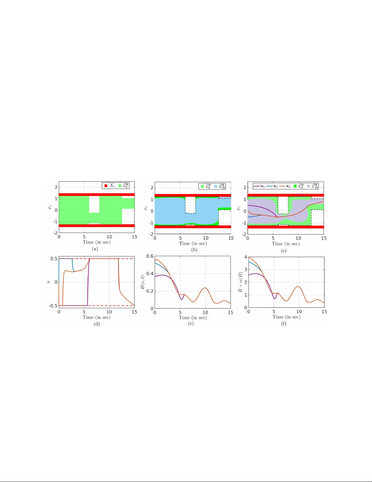
Neural Control Barrier Function s f or Signal T emporal Logic Specificat ions with Inpu t Co nstraints ∗ V aishnavi Jagabathula Centre f or Cyber-Physical Systems IISc, Bengaluru , In dia vaishnavij@i isc.ac.in Pushpak Jagtap Centre f or Cyber-Physical System s IISc, Bengaluru , In dia pushpak@iisc .ac.in March 1 8 , 2 026 A B S T R A C T Signal T emporal Log ic (STL) provides a powerful framework to d escribe complex tasks in v olving temporal and logical b ehavior in dynamical systems. This work addresses co ntroller synthe sis for continuo us-time system s subject to STL specifications and input constrain ts. W e propose a n eu- ral network-b ased framework for synthesizing time-varying co ntrol barrier fun ctions (TVCBF) and their correspon ding controller s for systems to fulfill a f r agment o f ST L specifications wh ile resp e ct- ing input constrain ts. W e f ormulate barrier condition s incor porating the spatial and tempora l logic of the given STL specification. W e also inc o rpora te a method to refin e the time-varying set that satisfies the STL specification for the given in put c o nstraints. Additionally , we introdu c e a validity condition to provid e formal safety g uarantees across the en tire state space. Finally , we d emonstrate the effectiveness of the pro posed appr o ach thro ugh several simulation studies co nsidering different STL tasks fo r various d ynamical systems (inc lu ding affine and non- affine systems). 1 Intr oduction Real-world dynamical systems requ ire co ntrol method s that en sure safety while executing inc reasingly complex tasks. Sign al T emp o ral L ogic (STL) [1] p rovides a formal lan guage for specifying such tasks along with quan titativ e robustness measures. A co mmon appro ach is to encod e STL spe cifications as mixed-integer lin ear con straints and solve them via MILP [2, 3, 4]; related methods using Bézier -curve c o nstraints achie ve similar results [5]. While effecti ve, these methods suf fer from high comp utational cost and limited scalab ility . Other appr o aches [6] successfully incorpo rated model predictive con trol with a smaller optimizatio n horizo n to solve STL tasks. Howe ver , they do not scale well in continu ous optimization p r oblems. Recen tly , reinforcem ent-learnin g-based methods [7, 8, 9] embed STL robustness in to reward f u nctions, av oiding explicit o ptimization; howe ver , they still face scalability issues an d lack f ormal safety gu arantees. Control b arrier functions (CBFs) are widely used to enforce certified safety [10, 11]. The system’ s safety is established by enfor c in g the inv ariance of a safe set, a zero superlevel set of CBF , and by designin g a con troller to keep the system trajectory inside the safe set. Since STL c ontains tem poral c o nstraints and stan dard CBFs are time-inv ariant, th ey cannot dire ctly cap ture time-varying ST L predic a tes. Time-varying CBFs have bee n propo sed for STL satisfaction [12, 13], including e xtensions to multi-agent s ystems [14]. Th ese ap proach e s ty pically req uire hand-crafted CBF templates for each STL interval and rely on quad r atic program s that m ay become infeasible unde r strict in put constraints. For instance, the system starting from a state ou tside an unsafe set would not be able to satisfy the STL specification within the specified time du e to the gi ven inp ut co nstraints. But in the existing li terature, either the states ar e presumed to be safe in itial states simp ly b e cause th ey are not explicitly in the un safe region, or a very small initial state set is co nsidered. In either case, solving the hand- crafted CBF tem plate using a quadr atic pr ogram would be infeasible un der input c onstraints. Additio nally , these works fo cus on con tr ol-affine sy stems and o n fragments ∗ This work was suppo rted by Siemens fellowship. of STL specifications that do n o t consider disjunctions. Related work in [15, 1 6 ] addresses STL satis faction for linear systems under input constraints, eith er by en coding STL into CBFs and computing least-v iolating controls [15] or by on lin e parameterization of time-varying CBFs [16]. While pr omising, these method s are lim ited to linear system dynamics. I n co ntrast, we dev elop a fr amew ork ap p licable to any general continuo us-time system (includ ing non-affine sy stems), th e r eby expanding th e class of s ystems for which STL specifications can be e n forced under bound ed inp uts. Recent dev elopmen ts in neural network-based and data-driven CBF [17, 18] hav e elim inated the need for han dcrafted CBF templates, but they focus on time- inv ariant settings and can not be trivially extended to h andle temporal STL pre d icates. T o the best o f o ur k nowledge, this is th e first work to add ress th e prob lem of contro ller synthesis for a class o f STL task s withou t relyin g on p redefined CBF temp lates and refinin g the time-varying set that satisfies the ST L task wh ile ensu r ing inp ut constrain ts. This letter considers c ontinuo us-time systems with a fr agment o f STL tasks sub jected to in p ut co nstraints. W e propo se a co ntrol strategy that ensures STL satisfaction un der input co nstraints. W e iteratively co nstruct time- varying sets that encode the STL semantics, keeping the input constrain ts into consid eration, and also formulate con trol barrier c o nditions over those sets. W e leverage the ap proxim ation c apability of neural n etworks to d ev elop a n eural network-based time-varying contro l barrier function and an associated neu r al network-based co ntroller for the given STL specifications und er input constraints. Since neur a l netw orks are trained on finite sample datasets, we also provide fo rmal g uarantees over the e ntire state spa ce by proposing a validity condition that ensures STL satisfaction. W e validate the effectiv eness of the pr oposed framework by applyin g it to various contin uous-time systems, each with different STL specifications and con trol limits. Our main contr ibutions are as follows: • W e addr ess the contro ller design proble m for a fragment of STL specificatio n s under input constrain ts. • W e pro pose a unified f ramework that (i) itera tively constructs tim e - varying sets en coding STL specification s, (ii) f ormulates a tim e-varying control bar rier fun ction (T VCBF) over the constructed sets. • W e develop a neur al network-ba sed TVCBF along with a neura l network con tr oller to enfor ce STL satisfac- tion. W e also der i ve a validity condition th at en sures STL satisfaction over the entire state space, despite training th e n e ural network s on a finite d a taset. • Finally , we demon stra te the effecti veness of our prop osed work on multiple continuo u s-time systems (includ- ing affine and n o n-affine systems) subjecte d to STL specification and input constraints. This paper is organiz e d as follows: Section 2 pr esents the class of system s we focu s on, introd uces signal temporal logic specifica tio n, and presents the p roblem we add ress in this p aper . Sectio n 3 presen ts the detailed f ormulatio n of time- varying CBF (TVCBF) fo r a contin uous state space and th en intro duces the neur a l n e twork-based TVCBF for a finite samples from the state-time space. It also provide s th e oretical guarantees for STL satisfaction u sing th e neural TVCBF designed over th e sampled points to extend it to th e continu ous state space. In Section 4, we describe the n eural ne twork ar c hitecture an d the training algorithm f o r neu r al networks (b oth TVCBF and controller network s) and th e n provide the strategy of iteratively construc ting and refining a continu ously differentiable time-varying set that encodes the ST L specifications. Finally , in Section 5, we provide simu lation r esults for various co ntinuou s-time systems. Section 6 c onclude s the paper with a summa r y . 2 Pr eliminaries and Problem Formu lation Notatio ns: The sets of real a nd non-negative real numbers are denoted by R and R ≥ 0 , resp e c ti vely . The set of natural numb ers be tween 1 to N is denoted by [1; N ] . An n -d imensional vector space is R n and a co lumn vector is x = [ x 1 , ..., x n ] ⊤ ∈ R n . Th e symb ol  deno te s elem ent-wise inequ ality of vector s. W e deno te a set of rea l matrices with n rows and m colu mns by R n × m . A con tinuous function α : ( − a, b ) → R fo r a, b > 0 is ca lled an extended class K function if it is strictly increasing, α (0) = 0 and it is denoted as K e . Th e no tation for partial d ifferentiation of a fu nction f : R n × R → R with respect to the variables x ∈ R n and t ∈ R is ∂ f ∂ x and ∂ f ∂ t , respectively . The p -nor m is represented using || · || p . An ind icator fu nction 1 x ∈ X = 1 , if x ∈ X , and 0 otherwise. A Lipschitz continu o us fu n ction f has a Lipschitz constant L ∈ R ≥ 0 if || f ( x 1 ) − f ( x 2 ) || 2 ≤ L || x 1 − x 2 || 2 . 2.1 System Descriptio n Consider a co ntinuou s-time nonlinear co ntrol system Σ : ˙ x ( t ) = f ( x ( t ) , u ( t )) , (1) where x ( t ) ∈ X , u ( t ) ∈ U are the state an d input of th e system at time t ∈ R ≥ 0 , and X ⊂ R n , U ⊂ R m are assum ed to be compact sets represen ting state and input co nstraints. Th e functio n f : X × U → R n is known a n d assumed to be a Lipschitz c ontinuo us fu nction with respect to x, u over X , U , with Lipsch itz constants L x , L u , respectiv ely . Let us define a state tra je c tory starting from x 0 with th e input signal u as x x 0 , u . 2.2 Signal T empora l Logic ( STL) Signal T emporal L ogic (STL) provides a for mal lan g uage fo r spec if ying spatial, temporal, and logical p roper ties [1]. An STL formu la is co mposed of predicates co mbined with tempor al and log ical op erators. Let x : R ≥ 0 → X ⊆ R n be a time-varying signal, and a predicate func tion h : X → R . A predica te is µ = true if h ( x ( t )) ≥ 0 , and false , otherwise. Th e b a sic STL fo rmulas are as follows: φ ::= true | µ |¬ φ | φ 1 ∧ φ 2 | φ 1 ∨ φ 2 |  [ a,b ] φ | ♦ [ a,b ] φ | φ 1 U [ a,b ] φ 2 , where µ is a predicate, the operato rs ¬ , ∧ , and ∨ represent the logical negation, co njunctio n , and disjunctio n operators, respectively . The temporal ope rators  , ♦ , and U me a n ‘ Always’, ‘Eventually ’ , an d ‘Until’ oper ators. The set [ a, b ] ⊂ R ≥ 0 is th e time interval in wh ich the temp oral operator s are activ e. T he fo rmal semantics o f can be found in [1]. Th e degree to which a signal x satisfies an STL specification φ at time t is quantified by the r obustness me a su re, denoted as ρ φ ( x , t ) ∈ R . For the STL formulae, the robustness seman tics are defined as: ρ µ ( x , t ) = h ( x ( t )) , ρ ¬ φ ( x , t ) = − ρ φ ( x , t ) , ρ φ 1 ∧ φ 2 ( x , t ) = min  ρ φ 1 ( x , t ) , ρ φ 2 ( x , t )  , ρ φ 1 ∨ φ 2 ( x , t ) = max  ρ φ 1 ( x , t ) , ρ φ 2 ( x , t )  , ρ  [ a,b ] ϕ ( x , t ) = min t ′ ∈ [ t + a,t + b ] ρ ϕ ( x , t ′ ) , ρ ♦ [ a,b ] ϕ ( x , t ) = max t ′ ∈ [ t + a,t + b ] ρ ϕ ( x , t ′ ) . W e say a signal x satisfies the STL spe cification, deno te d by ( x , 0) | = φ iff ρ φ ( x , 0) ≥ 0 . For b revity , we deno te ρ φ ( x ) ≥ 0 ≡ ρ φ ( x , 0) ≥ 0 and x | = φ ≡ ( x , 0 ) | = φ th r ough o ut the paper . For a contro l system in (1 ), an STL specification φ is satisfiable fro m the initial state x 0 ∈ X if there exists an inpu t signal u such that ρ φ ( x x 0 , u ) ≥ 0 . 2.3 Problem Formulation In this paper, we co nsider the fo llowing STL frag ment: ϕ ::= true | µ |¬ ϕ | ϕ 1 ∧ ϕ 2 | ϕ 1 ∨ ϕ 2 , (2a) φ ::=  [ a,b ] ϕ | ♦ [ a,b ] ϕ, (2b) Φ ::= N ^ i =1 φ i , (2c) where φ i , i ∈ { 1 , ..., N } are STL form u las defin ed for the in terval [ a i , b i ] is of the fo r m φ . The final STL syntax is o f the f orm Φ , su c h tha t ∪ N i [ a i , b i ] ⊆ [0 , T ] , wh e re T is the total time d uration covered by th e STL specification Φ . For the STL formu la e mentione d in (2 c), the r o bustness semantics can b e d e fined as ρ Φ ( x ) = min i ∈{ 1 ,...,N } ρ φ i ( x ) . Problem 1. Given an STL spec ification Φ of the form (2 c) for a time duration of [0 , T ] for a continuo us-time nonlin ear contr ol system Σ in (1) , ou r objec tive is to synthesize a contr oller u ( t ) = g ( x ( t ) , t ) (if it exists ) that ensures the system trajectory x x 0 , u starting a t x 0 satisfies the sp ecification Φ un der inpu t con straints U ⊂ R m . This letter prop oses a fr amework that iteratively constru cts time-varying sets enc o ding the given STL sp e c ification and co-design s a time- varying contro l barrier fun ction an d controller to keep the system with in these sets un der inp ut constraints, th ereby en suring ST L satisfaction. T o eliminate the need to prede fine the barrier and contro ller templates, we employ a neur al network (NN) app roach. 3 T ime-varying Control Barrier F unction This work designs a co n troller u sin g control barrier fu nctions to satisfy the STL task of th e fo rm (2c). Because the STL specification im p oses both tempo ral an d spatial c onstraints, time-varying co ntrol barrier fu n ctions (TVCBF) are required . This section reviews TVCBFs, wh ich gu a r antee STL satisfaction f or continuo us-time systems. 3.1 Time-V arying Control Barrier Function The time-varying control barrier fu nction-b ased a pproach is used to synthesize a con troller that ensur e s that the system trajectory stay s in sid e a time- varying set for a ll time. W e define a n augm ented set W = X × [0 , T ] , where X ⊆ R n and time in terval [0 , T ] , T ∈ R ≥ 0 . Definition 1. T ime-varyin g Contr o l Barrier Fun ction (TVCBF): A co n tinuously differ en tiable time-varying function B : W → R is a contr ol barrier fu nction for a contr ol system Σ in (1) , if for a time-va ryin g set C ( t ) ⊂ W , ther e exists a co ntinuou s function g : W → U su ch th at ∀ ( x, t ) ∈ C ( t ) , B ( x, t ) ≥ 0 , (3a) ∀ ( x, t ) ∈ W \ C ( t ) , B ( x, t ) < 0 , (3b) ∀ ( x, t ) ∈ W, ∂ B ∂ x f ( x, g ( x, t )) + ∂ B ∂ t ≥ − α ( B ( x, t )) , (3c) for some cla ss K e function α . Theorem 1. F or a co ntinuou s-time co n tr o l system Σ in (1) and a time-va ryin g set C ( t ) , supp ose th er e exist a con- tinuously differ entiable functio n B : W → R and a co ntr o ller g : W → U satisfying cond itio ns (3a) - (3c) . Then, the system trajectory x x 0 , u starting fr om ( x 0 , 0) ∈ C (0) with u ( t ) = g ( x ( t ) , t ) , will a lways stay in C ( t ) , i.e., x x 0 , u ( t ) ∈ C ( t ) , ∀ t ∈ [0 , T ] . Pr o of. Assuming that th e system starts at ( x 0 , 0) ∈ C (0) implies B ( x 0 , 0) ≥ 0 (as p er (3a)). Now , co nsidering condition (3c), there exists a co n trol signal g ( x ( t ) , t ) such that ˙ B ( x ( t ) , t ) ≥ − α ( B ( x ( t ) , t )) , where α ( · ) is a class K e function . Suppose b ( t ) = B ( x ( t ) , t ) , then ˙ b ( t ) ≥ − α ( b ( t )) . L et β be the solutio n of the equ a tio n to ˙ β ( t ) = − α ( β ( t )) , and β (0) = b (0) . Using Comp arison lemma [19, Chapter 3], b ( t ) ≥ β ( t ) , ∀ t ∈ [0 , T ] . Since b (0) ≥ 0 , and β ( t ) is non- negativ e fo r all t , we have b ( t ) = B ( x ( t ) , t ) ≥ β ( t ) ≥ 0 , ∀ t ∈ [0 , T ] . Ther efore, we conclu de that ( x ( t ) , t ) ∈ C ( t ) , ∀ t ∈ [0 , T ] (By Definition 1). 3.2 TVCBF for STL Specificatio ns Let u s consider th e STL specification Φ o f the form (2c ) be d efined over the time interval [0 , T ] , an d each φ i , i ∈ { 1 , ..., N } , is a n ev entually or always operator with th e correspo nding time in terval [ a i , b i ] . Let us denote the set of STL sub-f o rmulae with the eventually operator as Φ ♦ = { φ i | φ i = ♦ [ a i ,b i ] ϕ i } , a nd the sub- f ormulae with the a lways operator as Φ  = { φ i | φ i =  [ a i ,b i ] ϕ i } , su ch th at ∪ N i =1 I i ⊆ [0 , T ] , wh ere I i =  [ a i , b i ] , if φ i ∈ Φ  , [ t ∗ , t ∗ + δ ] ⊂ [ a i , b i ] , if φ i ∈ Φ ♦ . (4) The variables t ∗ , δ are selected such that: a i ≤ t ∗ < t ∗ + δ ≤ b i , and δ > 0 . The set of all acti ve pr e dicate componen ts of the STL for mula at time t is given by Φ a ( t ) = { ϕ i | t ∈ I i } . Assumption 1. W e a ssume that a t least one pr edicate is a ctive a t any given time, i.e., Φ a ( t ) 6 = ∅ , ∀ t ∈ [0 , T ] , on accoun t of th e state spa ce co nstraints imposed on the system. W e set one o f the STL sub-f ormulae describing state sp ace con straints for th e state x ∈ X in the entire time d uration [0 , T ] , w ith out compro mising on th e given STL task , resulting in an STL fo rmula of the form: Φ =  [0 ,T ] ( D || x − x c || p ≤ 1) ∧ Φ 1 , (5) where x c is the cen ter of the state spa c e co nstraint A ⊂ X , || · || p denotes p -no rm with p = 1 , 2 , ∞ , the con stant D = 1 / r , f or a circu lar state spac e con straint of radiu s r , D = diag (1 /w i ) is a diago nal matrix for a r ectangular state space b o und with w i as h alf the width of the constraint alo ng each state dimension of A ⊂ X , and Φ 1 is o f the for m (2c). W e n ow take the aug m ented set for finite-tim e W = X × [0 , T ] and define the time-d ependen t set of states that satisfy the STL specification as follows: S Φ ( t ) = { ( x, t ) ∈ W | min ϕ i  ρ ϕ i ( x )  ≥ 0 , ∀ ϕ i ∈ Φ a ( t ) } , (6) where ϕ i is th e non- te m poral predicate o f th e fo rm (2a). Theorem 2. F or a co ntinuou s-time contr ol system a s in (1) and an S TL specificatio n Φ of the form ( 2 c) satisfying Assumption 1 , sup p ose th a t there exist a co ntinuou sly differ entiable func tion B and a con tr oller g : X × [0 , T ] → U satisfying co nditions ( 3a) - (3c) in De fi nition 1, with so m e set C ( t ) = C Φ ( t ) ⊂ S Φ ( t ) , where S Φ ( t ) is d efined as ( 6) for STL specification Φ . Then, the system trajectory x x 0 , u starting fr om ( x 0 , 0) ∈ C Φ (0) with u ( t ) = g ( x ( t ) , t ) will alwa y s stay in C Φ ( t ) , i.e., x x 0 , u ( t ) ∈ C Φ ( t ) , ∀ t ∈ [0 , T ] , an d the STL specification Φ is satisfied by x x 0 , u , i.e., x x 0 , u | = Φ . Pr o of. By T h eorem 1, th e system tr ajectory startin g f rom ( x 0 , 0) ∈ C (0) u n der co ntroller g will always stay in C Φ ( t ) , i.e., x x 0 , u ( t ) ∈ C Φ ( t ) , ∀ t ∈ [0 , T ] . B y the constru ction of C Φ ( t ) ⊂ S Φ ( t ) in (6), we have min ϕ i  ρ ϕ i ( x ( t ))  ≥ 0 , ∀ ϕ i ∈ Φ a ( t ) , ∀ t ∈ [0 , T ] . This implies that th e robustness c o rrespon ding to acti ve STL fragmen ts at each time is positive; co nsequently , x x 0 , u | = Φ . 3.3 Neural Ne t work-based Time-V arying CBF ( N-TVCBF) In this section, we syn thesize TV CBF alon g with the con tr oller for a system to satisfy an STL specification . The set S Φ ( t ) form ed u sing (6) is not con tinuously differentiable, and the refore we still have a ma jor challenge to constru ct a set C Φ ( t ) ⊂ S Φ ( t ) in wh ich the barrier f unction B ( x, t ) is co ntinuo u sly differentiable. Ad ditionally , due to inp u t constraints, the trajector y x x 0 ,u ( t ) , starting at some x 0 ∈ S Φ (0) m ig ht leav e the STL safe set S Φ ( t ) at so m e time t ∈ [0 , T ] an d therefor e not satisfy the specification Φ . W e p r opose an iterati ve refinem e nt app roach in the n ext section to co n struct a set th at ensu r es STL satisfaction, alo ng with feasibility with respect to in put con stra ints and continuity in time . In this section, we focus on TVCBF assuming tha t the ap propr iate time-varying set C Φ ( t ) is av ailable. Lemma 1. The con tin uous-time system Σ in (1) with trajectory starting fr om ( x 0 , 0) ∈ C Φ (0) satisfies the STL specification Φ if the following co nditions hold with η ≤ 0 . max( q k ( x, t )) ≤ η , k ∈ [1; 3] , ∀ ( x, t ) ∈ W, (7) wher e q 1 ( x, t ) = −B ( x, t ) 1 ( x,t ) ∈C Φ ( t ) , q 2 ( x, t ) = ( B ( x, t ) + λ ) 1 ( x,t ) ∈ W \C Φ ( t ) , q 3 ( x, t ) = − ∂ B ∂ x f ( x, g ( x, t )) − ∂ B ∂ t − α ( B ( x, t )) , (8) and λ > 0 enforces strict ineq uality in (3b) . Pr o of. The first inequality f or q 1 with η ≤ 0 en su res that the CBF B ( x, t ) ≥ 0 in ( x, t ) ∈ C Φ ( t ) . Additionally , q 2 with η ≤ 0 ensures a strict negative value of CBF in ( x, t ) ∈ W \ C Φ ( t ) . Th e inequ ality q 3 with η ≤ 0 ensures the co nfinement of the system trajecto ry within the set C Φ ( t ) . Using Theo r em 1 an d 2, all the se in equalities togeth er ensure that a system trajectory starting fro m ( x 0 , 0) ∈ C Φ (0) with u ( t ) = g ( x ( t ) , t ) satisfies the STL specification Φ . One major cha llenge in solving these inequ a lities is the infinite n umber of con straints resulting from the continuo us state-space. T o overcom e this, w e use a finite number of samples f r om the set W . W e gener a te a set o f N samples s ( r ) = ( x, t ) ( r ) , wh e r e r ∈ [1; N ] , such that ∀ ( x, t ) ∈ W , ∃ s ( r ) ∈ W, || ( x, t ) − s ( r ) || 2 ≤ ǫ. (9) Now , we co nsider the set ˜ S Φ ( t ) = { s ( r ) | s ( r ) ∈ S Φ ( t ) , r ∈ [1; N ] } . A smaller value of ǫ ensur e s dense samplin g such th at ˜ S Φ ( t ) ∩ S Φ ( t ) 6 = ∅ . W e assume that we have the set ˜ C Φ ( t ( r ) ) ⊂ ˜ S Φ ( t ( r ) ) wh ich is a zero- superlevel set of B (( x, t ) ( r ) ) . In addition , instead of pre-d efining the TVCBF and con tr oller temp late, we ap prox im ate them with NNs and denote them as B θ 1 and g θ 2 , both p arameterized b y th e train able par a m eters θ 1 and θ 2 , respectively . Assumption 2. Th e candid ate N-TVCBF B θ 1 and its derivative a r e assumed to be Lipschitz continu o us with Lipschitz constants L b and L db , r e sp ectively [20]. Th e c o ntr oller NN g θ 2 has the Lipschitz constant L g . Addition ally , the 2- n orm of partial derivatives || ∂ B ∂ x , ∂ B ∂ t || 2 , fun ction f ( x, u ) a r e bounded by M b , M f r espectively , i.e., sup x,t || ( ∂ B ∂ x , ∂ B ∂ t ) || 2 ≤ M b , sup ( x,u ) || f ( x, u ) || 2 ≤ M f . Lemma 2 . [19, Ex. 3.3] If two functio ns h 1 and h 2 ar e Lipschitz c o ntinuo u s with constants L 1 and L 2 , r esp ectively , and ar e b ound ed by sup || h 1 || 2 ≤ M 1 and sup || h 2 || 2 ≤ M 2 , th en th eir p r o duct h 1 h 2 is also Lipschitz co ntinuou s with Lipschitz constan t M 1 L 2 + M 2 L 1 . Theorem 3. Consider a continuou s-time co n tr o l system ( 1) with comp act state and inp ut sets X a nd U , and an S TL specification Φ o f the fo rm (2c) satisfying Assumption 1. W ith Assumption 2, the system trajectory x x 0 , u starting at x 0 and u ( t ) = g θ 2 ( x ( t ) , t ) , is said to satisfy Φ under th e time-v a rying barrier B θ 1 , co ntr oller g θ 2 trained over the sampled p o ints a s in (9) if the following holds with η + L ǫ ≤ 0 : max( q k ( s ( r ) )) ≤ η , k ∈ [1; 3 ] , ∀ s ( r ) ∈ W , ∀ r ∈ [1; N ] , (10) wher e ǫ is as defi ned in (9) , q 1 , q 2 , q 3 ar e as defined in (8) . The maximum of the Lipschitz consta nts of q k , k ∈ [1; 3] in (8) is L = max { L 1 , L 2 , L 3 } , wh e r e L 1 = L 2 = L b , L 3 = L db ( M f + 1) + M b ( L x + L u L g ) + αL b , an d the class K e function is a ssumed to be of the form α ( z ) = αz , α > 0 . Pr o of. First, we show that, un der condition η + L ǫ ≤ 0 , the con structed B θ 1 via solving the inequalities in (1 0) satisfy (3a)-(3c) for the entire state space X and time space [0 , T ] . Using (9), Assumption 2 , an d L emma 2, we ob tain: ( i ) ∀ ( x ( t ) , t ) ∈ C Φ ( t ) , ∃ s ( r ) ∈ ˜ C Φ ( t ( r ) ) , r ∈ [1; N ] , s.t., || ( x ( t ) , t ) − s ( r ) || ≤ ǫ q 1 ( x ( t ) , t ) = q 1 ( x ( t ) , t ) − q 1 ( s ( r ) ) + q 1 ( s ( r ) ) = ( −B ( x ( t ) , t ) + B ( s ( r ) )) − B ( s ( r ) ) ≤ L b ǫ + η ∗ ≤ L ǫ + η ∗ ≤ 0 . ( ii ) ∀ ( x ( t ) , t ) ∈ W \ C Φ ( t ) , ∃ s ( r ) ∈ W \ ˜ C Φ ( t ( r ) ) , r ∈ [1; N ] , s.t., || ( x ( t ) , t ) − s ( r ) || ≤ ǫ q 2 ( x ( t ) , t ) = q 2 ( x ( t ) , t ) − q 2 ( s ( r ) ) + q 2 ( s ( r ) ) ≤ L b ǫ + η ∗ ≤ L ǫ + η ∗ ≤ 0 . ( iii ) ∀ ( x ( t ) , t ) ∈ W, ∃ s ( r ) ∈ W , r ∈ [1; N ] , s.t., || ( x ( t ) , t ) − s ( r ) || ≤ ǫ q 3 ( x ( t ) , t ) = q 3 ( x ( t ) , t ) − q 3 ( s ( r ) ) + q 3 ( s ( r ) ) = − ∂ B ∂ x f ( x ( t ) , g ( x ( t ) , t )) − ∂ B ∂ t − α B ( x ( t ) , t ) + ∂ B ∂ x ( r ) f ( x ( r ) , g ( s ( r ) )) + ∂ B ∂ t ( r ) + α B ( s ( r ) ) − ∂ B ∂ x ( r ) f ( x ( r ) , g ( s ( r ) )) − ∂ B ∂ t ( r ) − α B ( s ( r ) ) ≤ M f L db ǫ + M b ( L x + L u L g ) ǫ + L db ǫ + αL b ǫ + η ∗ ≤  L db ( M f + 1) + M b ( L x + L u L g ) + αL b  ǫ + η ∗ ≤ L ǫ + η ∗ ≤ 0 . This imp lies that if conditio n (10) is satisfied wit h L ǫ + η ≤ 0 , so are the conditions in continuous space in (7). Therefo re, the N-TVCBF B θ 1 satisfies (3a) -(3c) and by Theorem 2, the controller ensur es STL specification Φ is satisfied. 4 T raining of N-TVCBF and Contr oller This section p resents the n e ural network architectu r e, the construction of set ˜ C Φ ( t ) , the lo ss fun ctions designed for the TVCBF constrain ts ( 3a)-(3c), and the training pr o cess used to ensure formal g uarantees. 4.1 Neural Ne t work Architecture W e deno te the neural network ( NN) arc hitecture as { n 0 , n c , { n l } l , n o } , consisting of an inpu t layer with n 0 neuron s, a custom layer with n c neuron s, l hidden layers of width n l , and an output layer of size n o . The custom layer Figure 1: Neu ral network a r chitecture introdu c es explicit cross-couplin g between the inpu ts t and x = [ x 1 , x 2 , ..., x n ] ⊤ ∈ X , e.g., { tx 1 , tx 2 , ..., tx n } , or { e a 1 t x 1 , e a 2 t x 2 , ..., e a n t x n } (c f. Figure 1), which facilitates th e TVCBF appr o ximation during tra in ing. Each lay er uses weights w i ∈ R n i +1 × n i , biases b i ∈ R n i +1 , and a smooth activ ation σ ( · ) (e.g., Sof tplus, T anh , Sigmoid, SiLU) to enable the c o mputation of partial derivati ves of the NN with respe ct to its input ( ∂ B ∂ x , ∂ B ∂ t ). The r esulting NN fu n ction is o btained by r ecursively app ly ing the activ ation fu n ction in the hidden laye r s. The ou tput of each lay er in the NN is g iv en as z k +1 = Σ k ( w k z k + b k ) , ∀ k ∈ { 0 , 1 , ..., l − 1 } , wh ere Σ i : R n i → R n i is Σ i ( z i ) = [ σ ( z 1 i ) , ..., σ ( z n i i )] with z i denoting the con catenation of outp uts z j i , j ∈ { 1 , 2 , ..., n i } of the neu rons in the i - th lay e r . For the N-TVCBF , the output is y N N ( z l ) = w l z l + b l , whe r eas for the con troller NN, wh ich is designed to satisfy the input constraints U = { u ∈ R m | lb  u  u b } , we boun d the ou tput between ‘lb’ and ‘u b ’ u sing the HardT anh activ ation fun ction as y N N ( z l ) = HardT an h ( w l z l + b l ) ub lb . Th e outpu t o f HardT anh ( x ) ub lb is lb if x < lb, or ub if x > u b, o r x , otherwise. The overall trainable p arameter o f the NN is θ = [ w 0 , b 0 , ..., w l , b l ] . For an n -d im ensional system with m in p uts, th e architecture s are: N-TVCBF B θ 1 : { n + 1 , 2 n + 1 , { n l } l , 1 } and controller g θ 2 : { n + 1 , 2 n + 1 , { n l } l , m } with trainable p arameters θ 1 and θ 2 . 4.2 T ra ining Algo rithm with Formal Guara ntees T o solve Problem 1, we jointly train two neur al networks to appr oximate the TVCBF B θ 1 and con troller g θ 2 so that the associa ted loss fu nctions fo r constrain ts (10) converge. This section sum m arizes the train ing algo rithm. INPUTS: System d ynamics Σ satisfyin g Assumptio n 2 and an STL specification satisfying Assumption 1 . STEP 1 : Gener ate N s amples, build the dataset ˜ S Φ ( t ) u sing Φ , and initialize ˜ C Φ 0 ( t ) = ˜ S Φ ( t ) . STEP 2: Select n umber o f training ep ochs, L ipschitz bo unds ( L b , L dB , L g ), M b , NN hyperpar ameters ( l , n l , activation function , o p timizer, schedule r ), te r mination criteria (con vergence o f L cbf to zer o o r maxim um epochs). In itialize i = 0 , λ > 0 , η = − L max ǫ , th e train able par a meters θ 1 , θ 2 , Γ . STEP 3 : Training starts here: (i) Crea te batches of train in g d ata f r om ˜ C Φ i ( t ) . (ii) Fin d ba tch lo ss L cbf = k 1 L 1 + k 2 L 2 + k 3 L 3 , with k 1 , k 2 , k 3 > 0 and L 1 ( θ 1 ) = X s ( r ) ∈ ˜ C Φ i ( t ) ReLU  − B θ 1 ( s ( r ) ) − η  , (11) L 2 ( θ 1 ) = X s ( r ) ∈ W \ ˜ C Φ i ( t ) ReLU  B θ 1 ( s ( r ) ) + λ − η  , (12) L 3 ( θ 1 , θ 2 ) = X s ( r ) ∈ W ReLU  − ∂ B θ 1 ∂ x ( r ) f  x ( r ) , g θ 2 ( s ( r ) )  − ∂ B θ 1 ∂ t ( r ) − α  B θ 1 ( s ( r ) )  − η  , (13) where ReL U ( z ) = max(0 , z ) , α ( x ) = αz , α > 0 . (iii) Update θ i 1 , θ i 2 using optimizer (AD AM) [21]. STEP 4: T o ensure Assumption 2 and train NNs that are Lipschitz bound ed, we use the L e mma adopted f rom [2 0, Lemma 4.1] and satisfy the linear matrix ineq ualities ( LMIs) co r respond ing to the Lipsch itz co nstants o f different networks. W e f ormulate the lo ss fu nction L M (Θ , Γ) = − c l 1 log det( M L b ( θ 1 , γ 1 )) − c l 2 log det( M L dB ( ˆ θ 1 , ˆ γ 1 )) − c l 3 log det( M L g ( θ 2 , γ 2 )) , (14) where Θ = [ θ 1 , θ 2 ] , c l 1 , c l 2 , c l 3 > 0 are weights fo r sub-loss LMIs, Γ = [ γ 1 , ˆ γ 1 , γ 2 ] and M L b ( θ 1 , γ 1 ) , M L dB ( ˆ θ 1 , ˆ γ 1 ) , M L g ( θ 2 , γ 2 ) are matrices corr espondin g to the bou nds L b , L dB and L g respectively , com- puted as p e r [2 0, Le mma 4 .1]. Using the com puted Lipschitz constants an d L max as g iv en in Theore m 3, we update η = − L max ǫ . STEP 5 : ( STLSafeSetR efinement ) At ev ery n -th epoch, update the set ˜ C Φ i ( t ( r ) ) = ˜ C Φ i − 1 ( t ( r ) ) \ { s ( r ) ∈ ˜ C Φ i − 1 ( t ( r ) ) | B θ 1 ( s ( r ) ) < 0 or || ( ∂ B θ 1 ( s ( r ) ) ∂ x ( r ) , ∂ B θ 1 ( s ( r ) ) ∂ t ( r ) ) || ≥ M b } , (15) where M b is the ma ximum value of || ( ∂ B θ 1 ( s ( r ) ) ∂ x ( r ) , ∂ B θ 1 ( s ( r ) ) ∂ t ( r ) ) || 2 (Assumption 2 ). For rest of th e epochs, we keep ˜ C Φ i ( t ( r ) ) = ˜ C Φ i − 1 ( t ( r ) ) . In this step, we let the sample s s ( r ) ∈ ˜ C Φ i − 1 ( t ( r ) ) that have e ith er negativ e ba rrier value or large g radient be excluded from ˜ C Φ i ( t ( r ) ) in next iteration. This results in a set in which the barr ier B θ 1 is continuo usly differentiable. In Figure 2(a)-(c), we plo t the initial safe set ( ˜ C Φ 0 ) and the refinem ent don e at 2 0th and 40th epochs. W e observe that th e set ˜ C Φ 40 ( t ) ⊂ ˜ C Φ 20 ( t ) ⊂ ˜ C Φ 0 ( t ) . A t the end o f trainin g , alth ough we have the input c o nstraints, a trajectory starting at the r efined safe set ˜ C Φ E pochs (0) will be ab le to rema in in the refined safe set ˜ C Φ E pochs ( t ( r ) ) . STEP 6 : I ncremen t i a nd rep eat STEPS 3–5 un til termin ation criteria is satisfied. STEP 7 : I f lo sses co n verge to zero (app roximately to 10 − 6 to 10 − 4 ), r eturn NNs B θ 1 , g θ 2 , else restart from STEP 1 . Remark 1. Th e algorithm lacks a general conver gence guarantee, but str ate gies like r ed ucing the discr etization parameter ‘ ǫ ’ (or increasing the number of samples)[22] or adjusting NN hyper-parameters (a r chitectur e, learning rate) [23] can impr ove conver gence of loss. Algorithm 1 NN T raining Input: System dynam ics Σ , STL specification: Φ Output: B θ 1 , g θ 2 , η 1: Create dataset ˜ S Φ ( t ) u sing Φ 2: Initialize ˜ C 0 Φ ( t ) = ˜ S Φ ( t ) 3: Select: Numb er of train in g ep ochs ‘ E pochs ’, NN h y perpar ameters ( l , n l , ac tivation functio n, o ptimizer, sched- uler), desired L ip schitz b ounds ( L b , L dB , L g ) , M b , k 1 , k 2 , k 3 , train in g ter mination criteria (until loss goe s to zero or maximum epochs is attain ed). 4: Initialize: i = 0 , λ > 0 , η = − L max ǫ , Trainable para meters ( θ 1 , θ 2 , Γ ) 5: for i ≤ E poch s (T raining starts her e ) do 6: Create b a tc h es of train ing data fro m ˜ C Φ i ( t d ) 7: Find b atch loss L cbf = k 1 L 1 + k 2 L 2 + k 3 L 3 using (1 1)-(13) 8: Use optimizer (such as ADAM [21]) to u p date θ i 1 , θ i 2 9: Find th e Lip schitz co nstants of the network s using the E CLipsE to o l [2 4] 10: Find LM I loss L M using (1 4) and op timize Γ . 11: Use th e co m puted Lipschitz con stants to upd a te η = − L max ǫ 12: STLSafeSetRefinement : Update th e set ˜ C Φ i ( t ) u sing (15) 13: return B θ 1 , g θ 2 , η Theorem 4 . Consider a continu ous-time system (1) , with compact state and in p ut sets X and U , and an STL spe cifica- tion Φ o f the fo rm (2c) , satisfying Assumption 1, over the time interval [0 , T ] . Let B θ 1 ( x ( t ) , t ) be the trained N-TVCBF with the co rr esponding co ntr oller g θ 2 ( x ( t ) , t ) , such that the lo ss L cbf [in Algo rithm 1, Step 3 , Line 7 ] is minimized. If the loss L cbf goes to zer o and L M (Θ , Γ) ≤ 0 , then starting at an y point in the set C Φ (0) ⊂ S Φ (0) , th e trained contr oller NN g θ 2 ensur es that the STL specifica tion is satisfied. Pr o of. The loss L cbf = 0 implies tha t the solution to the finite in equality con ditions is ob ta in ed with η = − L max ǫ < 0 (as taken in Algo r ithm 1- lin e 4 and up dated in Line 11) . Add itionally , th e loss L M (Θ , Γ) ≤ 0 implies the satisfaction of Assumption 2 with the pre defined L ip schitz co nstants. Hence, using Theo rem 3, the co ntroller g θ 2 ensures that the STL spec ification is satisfied wh en the system is initialized in ( x 0 , 0) ∈ ˜ C Φ (0) ⊂ ˜ S Φ (0) . 5 Simulation Results In this section , we validate th e prop osed method using mecanum , p endulu m, spacecraft and a non - affine scalar system simulations fo r various STL tasks. W e use K e function α ( x ) = αx , w h ere α > 0 . T h e NNs have fixed architec- ture parameter s n 0 , l , n l , n o (input size, nu mber of hidden layers, hidden- layer width , an d o utput size) and a smooth activ ation functio n in all hidden- layers. 5.1 Non-affine Syst e m W e conside r a contro l non- affine system of the form (1) ˙ x = a (sin x + tan u ) , (16) where a = 0 . 5 , input u is bou nded within [ − 0 . 5 , 0 . 5 ] . The neural networks B θ 1 , g θ 2 are trained to satisfy the following STL spec ification: Φ 1 =  [0 , 15] ( | x | ≤ π/ 3) ∧  [6 , 8] ( − π / 3 ≤ x ≤ − π / 15) ∧  [12 . 5 , 15] π / 15 ≤ x ≤ π / 3) . (1 7) The state space is X = [ − π / 2 , π / 2] . The d iscretization parameter fo r da ta sampling is ǫ = 0 . 00 1 . The set ˜ S Φ ( t ) Figure 2: ST L Safe set refinem ent dur in g tr aining at epoch i = 0 , 20 , 40 is shown in g reen ( ˜ C Φ 0 ), light b lu e ( ˜ C Φ 20 ) and light p urple color ( ˜ C Φ 40 ), re sp ectiv ely . The system (16) satisfying Φ 1 (17) with state trajecto ry starting at x 1 (0) = 0 . 5 (purp le), x 2 (0) = − 0 . 5 ( blue), x 3 (0) = 0 . 1 (brown), N-TVCBF B θ 1 ( x ( t ) , t ) and contr o ller g θ 2 ( x ( t ) , t ) satisfies (3a)-(3c), keeping co ntrol input within limits (dotted red lines) is generated b y the p redicates f ormed usin g the STL Φ 1 (Refer to Section 3. 3 and 4. 2). For exam ple, ∀ t ∈ [6 , 8 ] , the ac tive pred icate is ρ Φ 1 ( x , t ) = min  ( − π / 15 − x ) , ( x + π / 3 ) , ( π / 3 − | x | )  , and ∀ t ∈ [12 . 5 , 15] , the active predicate is ρ Φ 1 ( x , t ) = min  ( π / 3 − x ) , ( x − π / 15) , ( π / 3 − | x | )  , whereas for th e entire time, the active p redicate is ρ Φ 1 ( x , t ) = π / 3 − | x | . W e fix the architecture o f the neural networks as NCBF: { 3 , { 64 } 3 , 1 } , and NN co ntroller: { 3 , { 64 } 3 , 1 } with Si gmoid Linear Unit (SiLU ) as ac tivation function . W e choo se a cu stom layer to represent the cross-coup ling terms as { e − t x }. The tr aining algorithm conv erges to obtain the neural n etworks with η ∗ = − 0 . 02 , satisfying Theorem 4 . In Figure 2(a)-(c), we sh ow th e initial safe set ( ˜ C Φ 0 ) in gree n color and its refinement at ep och i = 20 (ligh t blu e co lo r), and at epoch i = 4 0 ( light p urple c o lor) wh ile train in g the neur a l networks. W e observe that the set ˜ C Φ 40 ( t ) ⊂ ˜ C Φ 20 ( t ) ⊂ ˜ C Φ 0 ( t ) . A t the en d of trainin g, althoug h we have the input constraints, a trajectory starting at the re fin ed safe set ˜ C Φ E pochs (0) will be able to rem a in in the refined safe set ˜ C Φ E pochs ( t ( r ) ) . W e also observe in Figure 2(c) that f or different in itial states x 1 (0) = 0 . 5 , x 2 (0) = − 0 . 5 , x 3 (0) = 0 . 1 , the trajectories satisfy the specification Φ 1 . The con trol inpu ts for the three trajecto ries lie within the safety limits (do tted red lin es), as seen from Figure 2( d). Additionally , the barr ier cond itions (3a), (3c) are satisfied as seen in Figur es 2(e),( f ) with α = 5 . 5.2 Mobile robot-Mecanum W e conside r an example of a mo bile robo t with the following mecanum drive dynamics of the form (1): ˙ x =  ˙ x 1 ˙ x 2  =  u 1 u 2  , (18) where x 1 , x 2 are th e x, y coor dinates and u 1 , u 2 are the velocity inputs, bound e d within [ − 0 . 2 , 0 . 2] . The neu ral networks B θ 1 , g θ 2 are tr ained to satisfy the following STL specification : Φ 2 =  [0 , 15] ( || x || 2 ≤ 1 . 6 ∧ || x − x u || 2 > 0 . 3) ∧  [12 , 15] ( || x − x g || 2 ≤ 0 . 3 ) , (19) where x is the rob ot’ s p o sition, x u = [1 , 0] ⊤ is the u nsafe region which the robot sho uld alw ays avoid, and x g = -2 -1 0 1 2 -2 -1.5 -1 -0.5 0 0.5 1 1.5 2 0 5 10 15 0 0.2 0.4 0.6 0.8 0 5 10 15 0 0.5 1 1.5 2 0 5 10 15 -1 0 1 0 5 10 15 -1 0 1 0 5 10 15 -0.2 0 0.2 0 5 10 15 -0.2 0 0.2 Figure 3: Mecanum satisfying Φ 2 (19) with state trajectories starting at [ − 1 , − 1 ] ⊤ (blue), [1 . 4 , − 0 . 3] ⊤ (purp le), N- TVCBF B θ 1 ( x ( t ) , t ) and con troller g θ 2 ( x ( t ) , t ) satisfying (3a)-(3c), keeping con trol inputs within limits ( d otted red lines) [0 , 0 ] ⊤ is the goal position that th e robo t should reach in the time interval [12 , 15] seco n ds. Th e state space X = [ − 2 , 2] × [ − 2 , 2] . The discretizatio n parameter for data samplin g is ǫ = 0 . 0 2 . For every ( x, t ) ∈ W , the set ˜ S Φ 2 ( t ) is gene r ated by the predicate s for m ed using the STL Φ 2 (Refer to Sectio n 3.3 and 4.2). For examp le, ∀ t ∈ [1 2 , 1 5] , the activ e pred ica te is ρ Φ 2 ( x , t ) = min  (0 . 3 − || x − x g || 2 ) , (1 . 6 − || x || 2 ) , ( || x − x u || 2 − 0 . 3)  , wh e r eas for the rest of the time, the acti ve predicate is ρ Φ 2 ( x , t ) = min  (1 . 6 − || x || 2 ) , ( || x − x u || 2 − 0 . 3)  . W e fix the neura l network architecture s as NCBF: { 3 , { 45 } 3 , 1 } and NN controller : { 3 , { 45 } 3 , 2 } , with T a n h activ ation function s in all hidden layers. W e chose th e custom layer to repr esent th e cro ss-coupling ter m s as { t x 1 , t x 2 } . The train in g algor ithm conv erges to obtain the n eural networks with a value of η ∗ = − 0 . 0 664 , satisfying The orem 4. As seen fro m Figure 3(a)-(c ), we observe that for different initial states x (0) = [ − 1 , − 1] ⊤ , x (0) = [1 . 4 , − 0 . 3] ⊤ , the trajecto ries satisfy th e STL spec ification Φ 2 by reaching the goal p o sition and staying there within the desired time in terval [12 , 15] secon ds, while always remaining in safe region. The contr ol inputs fo r th e thre e trajectories lie within the safety lim its (dotted red lines), as seen from Figu re 3(f),(g). Additionally , the barr ier conditio ns (3 a), (3c) are satisfied as seen in Figures 3(d),( e) with α = 2 . 5 . 5.3 Pendul um W e now con sider an example o f a p e ndulum with the following dyn amics: ˙ x =  ˙ x 1 ˙ x 2  =  x 2 u ml 2 − g l sin x 1 − b ml 2 x 2  , (20) where x 1 , x 2 are the ang le and an gular velocity of the p endulu m. The mass m = 0 . 5 kg, length of the rod l = 0 . 5 m , acceleration due to gr avity g = 9 . 8 m/s, an d the damp ing coefficient b = 0 . 1 . The external input u is th e torqu e, bound ed between [ − 12 , 12] . The STL sp e c ification for the p endulu m considered is as follows: Φ 3 =  [0 , 16] (0 ≤ x 1 ≤ π / 2 ∧ | x 2 | ≤ 2) ∧  [7 , 9] ( | x 1 − π / 3 | ≤ 0 . 2 ∧ | x 2 | ≤ 0 . 2) ∧  [14 , 16] ( | x 1 − π / 4 | ≤ 0 . 2 ∧ | x 2 | ≤ 0 . 2) . (21) T o meet the STL specification Φ 3 , the pendu lum should maintain x 1 = π / 3 , x 2 = 0 in the time interval [7 , 9 ] seconds with a tolera n ce of 0 . 2 . Subseq u ently , in the time interval [1 4 , 1 6] , the pendulum should be balan ced at the ang le x 1 = π / 4 , x 2 = 0 with a tolerance o f 0.2. The state space X = [ − 0 . 15 , π / 2 + 0 . 15] × [ − 2 . 15 , 2 . 15] . The states should always rem ain within X . The discretizatio n parameter for data sampling is ǫ = 0 . 06 . For every ( x, t ) ∈ W , the set ˜ S Φ 3 ( t ) is g e n erated by the pred icates formed u sing the STL Φ 3 (Refer to Section 3 .3 and 4.2). W e fix the architec tu re of the neura l networks as NCBF: { 3 , { 100 } 5 , 1 } , an d NN contro ller: { 3 , { 128 } 5 , 1 } with T anh ac ti vation function s in all h idden lay ers. W e chose the custom lay er to intro duce the cross-cou pling terms in the fo r m o f { e t x 1 , e t x 2 } . The training algor ithm c o n verges to obtain B θ 1 , g θ 2 with an op tim al value o f η ∗ = − 0 . 04 , satisfying T heorem 4. As seen from Figure 4 ( a) and (b), we ob ser ve that the STL specification Φ 3 is satisfied by implementin g the trained controller g θ 3 starting at d ifferent initial states. Th e contro l in puts for the thre e trajectories lie within the safety limits (do tted red lines), as seen in Figure 4(e) . Furthe r more, the barr ier condition s (3a), ( 3c) are satisfied as seen fro m Figures 4 (c), (d ) with α = 5 . 0 2 4 6 8 10 12 14 16 0 0.1 0.2 0.3 0.4 0.5 0.6 0.7 0.8 0 2 4 6 8 10 12 14 16 0 0.5 1 1.5 2 2.5 3 3.5 4 0 2 4 6 8 10 12 14 16 -15 -10 -5 0 5 10 15 0 2 4 6 8 10 12 14 16 0 0.2 0.4 0.6 0.8 1 1.2 1.4 1.6 0 2 4 6 8 10 12 14 16 -2 -1.5 -1 -0.5 0 0.5 1 1.5 2 Figure 4: Pendulum satisfying Φ 3 (21) with state trajectories startin g at d ifferent i nitial states [1 . 1 , 0 . 0 1] ⊤ (blue), [0 . 6 , 0 . 1] ⊤ (purp le), [0 . 4 , 0 . 0 1 ] ⊤ (yellow), N-TVCBF B θ 1 ( x ( t ) , t ) and contro ller g θ 2 ( x ( t ) , t ) satisfying (3 a)-(3c), keep- ing control in puts within lim its (do tted red lines) W e conside r a different STL specification Φ 4 of the f o rm (2c) with a disjun ction op erator as follows: Φ 4 =  [0 , 16] (0 ≤ x 1 ≤ π / 2 ∧ | x 2 | ≤ 2 ) ∧  [7 , 9]  ( | x 1 − π / 3 | ≤ 0 . 2 ∨ | x 1 + π / 4 | ≤ 0 . 2) ∧ | x 2 | ≤ 0 . 2  ∧  [14 , 16] ( | x 1 − π / 4 | ≤ 0 . 2 ∧ | x 2 | ≤ 0 . 2) . (22) 0 5 10 15 0 0.5 1 1.5 2 0 5 10 15 0 5 10 15 0 5 10 15 -1 0 1 0 5 10 15 -2 -1 0 1 2 0 5 10 15 -12 -6 0 6 12 Figure 5: T op r ow: Pen dulum satisfying Φ 4 with state tr a je c tories starting at different initial states represented in blue, brown, purple, o r ange, Bottom row: N-TVCBF B θ 1 ( x ( t ) , t ) and controller g θ 2 ( x ( t ) , t ) satisfying (3a)-(3c), keeping control inputs within lim its ( dotted r e d lines) The state space is X = [ − π / 2 − 0 . 15 , π / 2 + 0 . 15 ] × [ − 2 . 15 , 2 . 15 ] . T o meet th e STL sp e c ification Φ 4 , the pendulu m must keep x 1 at π / 3 or − π / 4 an d x 2 at 0 with a toleran ce of 0. 2 in the interval [7 , 9 ] seconds, then main tain x 1 = π / 4 a nd x 2 = 0 with a toleran ce of 0.2 in the interval [14 , 16] , while remaining in X for all t ∈ [0 , 16] . W e use discretization ǫ = 0 . 0 6 for data sam pling. For every ( x, t ) ∈ W , the set ˜ S Φ 4 ( t ) is g e nerated using predicates of φ 1 (see Section s 3.3 and 4.2). The N-TVCBF and co ntroller networks b oth uses NN arch itectures { 3 , { 64 } 3 , 1 } with a custom layer for in tr oducin g cross-coupling terms of the form { e t x 1 , e t x 2 } and T anh activ ation fun c tions in all hidden layers. W ith the value o f η ∗ = − 0 . 03 , the tr a in ing algo rithm co n verges to ob tain B θ 1 , g θ 2 , satisfying Theor em 4. The Figures 5 (a) ,(b) sh ow that the STL specification Φ 4 is satisfied b y implementing the trained co ntroller g θ 2 starting at different in itial condition s. The contro l inputs for the thre e trajec to ries lie within th e safety limits ( d otted red lines), a s seen fr om Figure 5( e ) . Fu rthermo re, the barrier conditions (3a), (3c) a r e satisfied as seen f rom Figur es 5 (c),(d ), with α = 5 . 5.4 Rotating Spacecraft Model Consider a ro tating rig id spa c e craft mo d el [19], whose dyna mics are governed by th e fo llowing set o f eq uations: ˙ x = " ˙ x 1 ˙ x 2 ˙ x 3 # =    J 2 − J 3 J 1 x 2 x 3 + 1 J 1 u 1 J 3 − J 1 J 2 x 1 x 3 + 1 J 2 u 2 J 1 − J 2 J 3 x 1 x 2 + 1 J 3 u 3    , (23) where x 1 , x 2 , x 3 are the angles abou t the p rincipal axes, the principal mome n ts of inertia are J 1 = 200 , J 2 = 200 , J 3 = 10 0 , and u 1 , u 2 , u 3 are the torque inputs bo unded in [ − 2 0 , 2 0 ] . The state spa c e is X = [ − 0 . 25 , 0 . 25] 3 . W e validated the pr oposed fram ew ork on an STL spe c ifica tio n: Φ 5 =  [0 , 15] ( || x || ∞ ≤ 0 . 2) ∧ ♦ [5 , 8] (0 ≤ x 1 ≤ 0 . 15) ∧ ♦ [12 , 15] ( − 0 . 15 ≤ x 1 ≤ 0) (24) The d iscretization pa r ameter fo r data samp lin g is ǫ = 0 . 03 . For ev ery ( x, t ) ∈ W , the set ˜ S Φ 5 ( t ) is gener a te d by th e predicates fo rmed u sing the STL Φ 5 (Refer to Section 3.3 and 4.2). W e fix the arch itecture of the NNs as N- T VCBF: { 4 , { 50 } 4 , 1 } , and NN co ntroller: { 4 , { 50 } 4 , 3 } with T anh acti vation func tions in all h idden layers. The custom layer for introdu cing cross-couplin g terms is of the f o rm { e t x 1 , e t x 2 } . T he tr aining algorith m con verges to obtain B θ 1 , g θ 2 0 5 10 15 0 0.5 1 1.5 0 5 10 15 0 5 10 0 5 10 15 -0.2 -0.1 0 0.1 0.2 0 5 10 15 -0.2 -0.1 0 0.1 0.2 0 5 10 15 -0.2 -0.1 0 0.1 0.2 0 5 10 15 -20 -10 0 10 20 0 5 10 15 -20 -10 0 10 20 0 5 10 15 -20 -10 0 10 20 0 0.1 0.2 0.3 0.2 0.3 0.4 0 0.1 0.2 0.3 2 4 Figure 6: (a)-(c) Spacecraft satisfying Φ 5 with state trajectories starting at different initial states repr esented in blue, brown, purple, (d)- (h) N-TVCBF B θ 1 ( x ( t ) , t ) and controller g θ 2 ( x ( t ) , t ) satisfying (3a)-(3c), keeping contr ol inp uts within limits ( dotted r ed lin es) with an value of η ∗ = − 0 . 03 , satisfying Theor em 4. The Figures 6 (a)-(c) show th at the trained controller g θ 2 enforce s the STL specification Φ 5 from d ifferent initial condition s. T he co rrespond ing co n trol inputs remain within the safety limits (do tted r e d lines) in Figures 6(e) – (g). In add ition, the barr ie r co n ditions (3 a) and (3c) are satisfied, as shown in Figures 6(d) a n d (h), with α = 7 . 6 Conclusion This study d emonstrates the synthesis of a for mally verified ne ural network- based controller that satisfies signal tem- poral log ic (STL ) specifications for co ntinuou s-time systems. This was achieved b y establishing a link between the time-varying con trol barrier fun ction ( TVCBF) and the STL sema n tics. W e formula te the TVCBF co nstraints as ap- propr iate loss fun ctions f or a finite-state space, compu te and re fine time-varying safe sets for STL satisfaction under input constra in ts, an d, tog ether with a validity co ndition, p rovide guarantees for a co ntinuou s state space. W e also validated th e neural network framework for different continuou s-time systems sub ject to fra g ments of different STL specifications and inp ut co nstraints. Refer ences [1] O. Maler and D. Nickovic, “Monito ring tempor al pr operties o f continuou s signals, ” in Internationa l Sympo sium on F ormal T echniqu e s in Re a l-T ime and F a ult-T olerant Systems . Springe r, 2004, pp . 152 –166. [2] V . Raman, M. Maasoumy , and A. Donzé, “Mo del p redictive co ntrol from sign al temporal logic specifications: A case study , ” in 4 th ACM SIGB ED I nternation al W orkshop o n Desig n , Modeling, and Evalu a tion o f Cyber- Physical Systems , 2 014, pp. 52 –55. [3] B. Ba¸ spinar, H. Balakrishnan , and E. K oyuncu, “Mission plannin g and contr o l of multi-a ir craft systems with signal tem poral lo gic sp e cifications, ” IEEE Access , vol. 7, pp. 15 5 941–1 55 9 50, 2 0 19. [4] S. Sadr a ddini and C. Belta, “Robust tempor al log ic model pr edictive con trol, ” in 5 3r d Annu al Allerton Confer- ence on Commun ication, Contr ol, and Computing (Allerton) , 2015, pp . 7 72–77 9. [5] J. V erhagen, L. Lindem a n n, and J. Tumov a, “T emp orally robust multi-ag ent STL motion planning in continuou s time, ” in IEE E America n Contr ol Confer ence (ACC) . IEEE , 20 24, pp. 251 –258 . [6] S. S. Farahani, V . Raman, and R. M . Murray , “Robust mo del p redictive control for signal tempo ral lo gic syn the- sis, ” IF AC-P apersOnLine , vol. 48, no. 2 7, pp. 323– 328, 2015. [7] D. Aksaray , A. Jones, Z. K ong, M. Schwager , and C. Belta, “ Q - learning for robust satisfaction of signal tempor a l logic specifications, ” in IEEE 55 th Confer ence on Decision and Co n tr o l (CDC) . IEEE , 2016 , pp. 6565 – 6570 . [8] N. Saxena, S. Gorantla, an d P . Jagtap, “Funnel- based re ward shaping fo r signal tempor al logic tasks in rein force- ment learning, ” IEE E Ro botics an d Automation Letters , vol. 9, no. 2, pp. 1 373– 1 379, 2024. [9] Y . Men g and C. Fan, “Signal tempor al logic neu ral p r edictive co ntrol, ” IEEE Rob o tics and Automation Letters , vol. 8, no. 1 1, p p. 77 19–7 7 26, 2023. [10] A. D. Am es, S. Coogan , M. Egersted t, G. Notom ista, K. Sreenath, an d P . T abuada, “Control barrier fu nctions: Theory and ap plications, ” in 18th Eur opean Contr ol Confer ence (ECC) , 201 9, pp . 34 20–3 431. [11] E. Shak hesi, A. Katrinio k, and W . P . M. H. M. Heemels, “Co u nterexample- guided synth esis of robust discrete- time co ntrol ba rrier fu nctions, ” IE EE Contr ol Systems Letters , vol. 9, pp . 157 4 –157 9, 20 25. [12] L. Lind emann and D. V . Dimarog onas, “Control bar rier function s for signal tempor al logic tasks, ” I EEE Contr ol Systems Letters , vol. 3, no . 1, pp. 96– 101, 2018. [13] A. Ruo, L. Sabattini, a n d V . V illani, “CBF-based motion planning for socially responsible robot na vigation guaran tee ing STL spe cification, ” in Eur opean Contr o l Conference (ECC) , 2024 , pp. 122–1 27. [14] L. Lin demann and D. V . Dimaro gonas, “Barrier func tio n b ased collab orative co n trol of multiple robo ts u nder signal tem poral logic tasks, ” IEE E T ransactio ns on Contr ol of Network Systems , vol. 7, no . 4, pp. 1916 –1928 , 2020. [15] M. Charitidou and D. V . Dimar ogonas, “Barrier functio n-based mod el predictive contro l under signal temporal logic specifications, ” in 202 1 Eur opean Contr o l Confe rence (ECC) , 2021 , pp. 734–7 39. [16] ——, “Reced ing horizon co ntrol with o n line barr ier fu nction design und er signal temp oral logic specificatio n s, ” IEEE T ransactions on Automatic Contr ol , vol. 68 , no. 6, pp. 3545 – 3556 , 2 023. [17] M. Anand an d M. Zam ani, “Form a lly verified n eural network contro l b arrier cer tificates f o r u nknown system s, ” IF A C-P apersOnLine , vol. 5 6, no . 2, pp . 243 1 –243 6, 20 23. [18] A. Ne jati a nd M. Zamani, “Data-driven synthesis of safety controller s via multiple control barr ier certificates, ” IEEE Contr ol Systems Letters , vol. 7, p p. 2497– 2502 , 202 3. [19] H. K. Khalil, Nonlinear Sy stems . Upper Sadd le River , NJ: Pr e ntice Ha ll, 2002. [20] A. Basu, B. S. Dey , and J. Pushpak, “Neural increm ental input-to -state stable control Lyapu nov fun ctions for unknown continu ous-time systems, ” arXiv p r eprint arXiv:250 4.183 30 , 20 25. [21] D. P . King m a and J. Ba, “ Adam : A metho d for stochastic o ptimization, ” arXiv p r eprint arXiv:1 412.6 980 , 2 014. [22] H. Zhao, X. Zeng, T . Chen , Z. Liu, an d J. W ood cock, “Learn ing safe neural network contr ollers with barrier certificates, ” F ormal Aspects of Computing , vol. 33, no. 3, p p. 437–4 55, 2021. [23] Y . Li, C. W ei, and T . Ma, “T owards explainin g the regularizatio n effect o f initial large learning rate in train in g neural n etworks, ” Advan ces in neural info rmation pr ocessing systems , vol. 3 2, 2 019. [24] Y . Xu and S. Siv aranjani, “ECLipsE: Efficient composition al Lipschitz con stant estimation for deep neur a l n et- works, ” Advan ces in Neural In formation Pr ocessing S ystems , vol. 37, p p. 10 414– 10 441, 20 24.