Demand Response Under Stochastic, Price-Dependent User Behavior

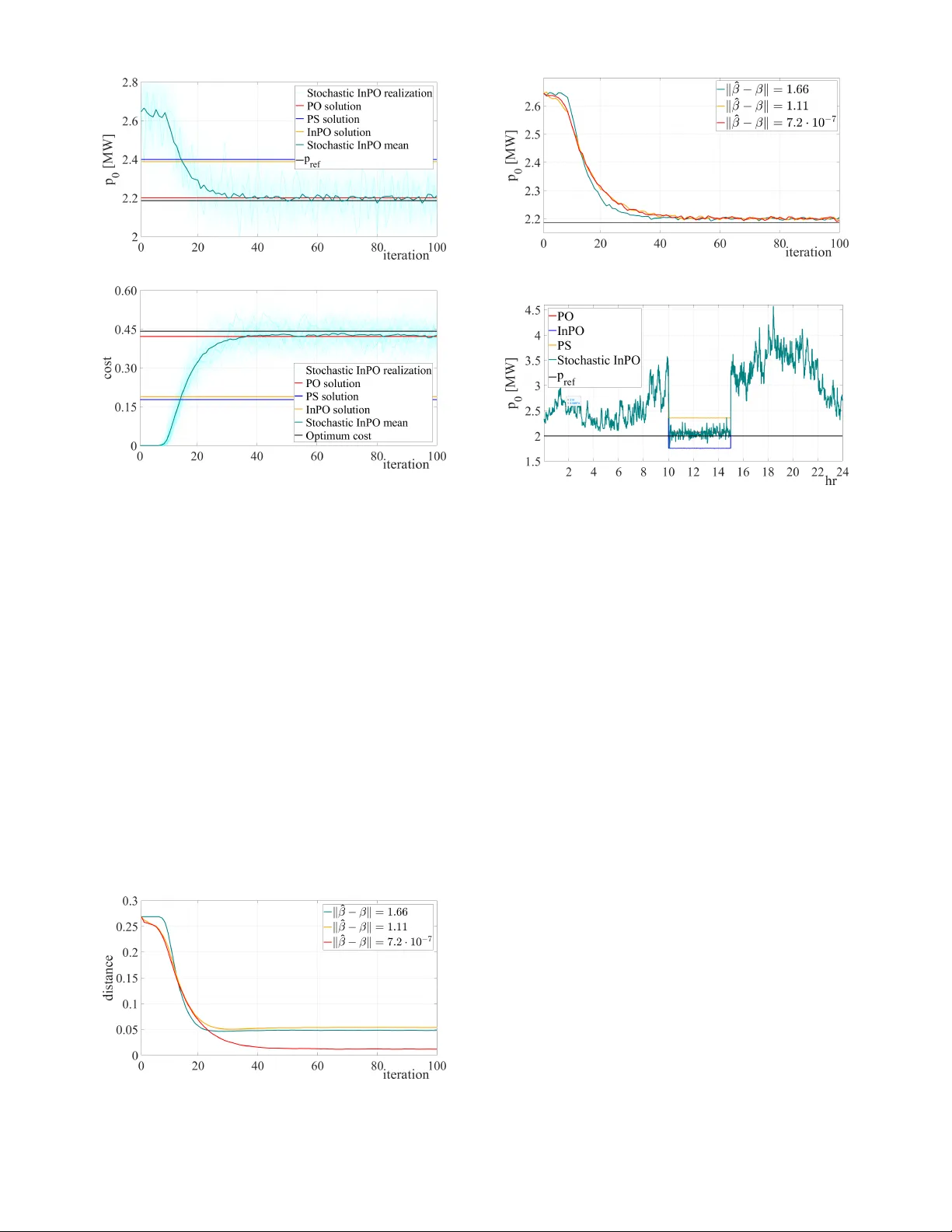
Demand Resp onse Under Sto c hastic, Price-Dep enden t User Beha vior Guido Ca vraro Andrey Bernstein Emiliano Dall’Anese Abstract— This pap er focuses on price-based residential demand resp onse (DR) implemen ted through dynamic adjust- men ts of electricity prices during DR even ts. It extends exist- ing DR mo dels to a sto chastic framework in whic h customer resp onse is represen ted b y price-dep enden t random v ariables, lev eraging models and tools from the theory of sto c has- tic optimization with decision-dependent distributions. The inheren t epistemic uncertain t y in the customers’ resp onses renders op en-loop, mo del-based DR strategies impractical. T o address this challenge, the paper prop oses to emplo y sto c hastic, feedback-based pricing strategies to comp ensate for estimation errors and uncertaint y in customer response. The paper then establishes theoretical results demonstrating the stability and near-optimality of the prop osed approach and v alidates its eectiv eness through numerical simulations. I. Introduction With the growing in tegration of diverse energy re- sources across the p o w er grid and the rapid electrication of m ultiple sectors, maintaining a reliable electricit y sup- ply has become increasingly challenging for utilities [1]. Residen tial demand response (DR) has long been a k ey instrument for system op erators (SOs) to manage extreme operating conditions, including peak load even ts and v oltage violations [2]. DR strategies v ary in b oth temp oral resolution and con trol mec hanisms, and are generally categorized into direct and indirect load control. In direct load control, SOs assume full authorit y ov er consumer loads during sp ecied p erio ds, mo difying consumption patterns in real time to address system-lev el contingencies. In contrast, indirect load con trol lev erages economic incen tiv es— either through dynamic pricing or predened monetary rew ards—to encourage consumers to volun tarily adjust their electricity usage. See, e.g., [3], for a comprehensive surv ey . Despite their p oten tial, the real-world eectiv eness of DR programs remains limited. Direct control schemes G. Ca vraro and A. Bernstein are with the Po wer Systems En- gineering Center, National Renewable Energy Lab oratory . email: guido.cavraro@nrel.go v, andrey .b ernstein@nrel.go v. E. Dall’Anese is ... This work w as authored by the National Renew able Energy Lab- oratory , operated b y Alliance for Sustainable Energy , LLC, for the U.S. Department of Energy (DOE) under Contract No. DE-A C36- 08GO28308. F unding provided by the NREL Lab oratory Directed Research and Developmen t Program. The views expressed in the article do not necessarily represen t the views of the DOE or the U.S. Gov ernment. The U.S. Gov ernment retains and the publisher, by accepting the article for publication, ac kno wledges that the U.S. Gov ernmen t retains a nonexclusiv e, paid-up, irrev ocable, w orldwide license to publish or repro duce the published form of this work, or allow others to do so, for U.S. Go vernmen t purp oses. often face lo w participation rates, as they may compro- mise user comfort or conv enience, requiring customers to accept reduced autonom y o ver their energy use [4]. Indi- rect con trol strategies, on the other hand, rely heavily on accurate mo deling of consumer b ehavior in resp onse to pricing or incentiv es. Inadequately designed price signals can inadverten tly cause adv erse eects, such as load sync hronization or system instabilit y , undermining the reliabilit y they are in tended to supp ort [5]. This pap er fo cuses on indirect load control, precisely on real-time price-based DR. Sp ecically , the SO dynam- ically mo dies electricit y prices during DR even ts. The classical approac h to mo deling user resp onse assumes a deterministic relationship b et w een price and con- sumption, often grounded in the assumption of rational user b eha vior (e.g., [6], [7]). Ho wev er, suc h assumptions are ov erly simplistic and fail to capture the inherent v ariability and uncertaint y in human decision-making. A common extension of deterministic mo dels intro- duces sto c hasticit y into the user resp onse—typically by adding xed noise terms [8]. Y et, this approach do es not account for the fact that consumer resp onsiv eness is inheren tly price-dep endent: as prices increase, a stronger reduction in demand is generally exp ected. T o address this limitation, w e propose a nov el framework that mo dels user b eha vior using price-dep endent random v ariables, drawing on to ols from the theory of stochastic optimization with decision-dep endent distributions; see the mo dels and algorithms in [9]–[14], the more recent w orks in [15], [16], and the survey [17]. One of the key challenges in implementing indirect, price-based DR strategies lies in the epistemic uncer- tain ty of user response. Specically , accurately esti- mating residential price elasticit y is dicult b ecause b eha vioral resp onses are small, confounded by many factors, and the data (price v ariation and the cor- resp onding consumption change) are limited [8], [18]. Moreo ver, factors suc h as num ber of household members, income, and o verall nancial situation aect the sensi- tivit y to prices [19]. Finally , dierent studies provide dieren t sensitivity results [20]. This inherent epistemic uncertain ty makes traditional op en-lo op, mo del-based approac hes infeasible in practice. Therefore, this paper adv o cates a sto chastic feedbac k-based pricing strategies to comp ensate for the uncertaint y in user resp onse and ensure robust p erformance. This pap er is structured as follows. In Section I I, w e presen t the pow er grid and DR mo dels. In Section I I I, w e formulate the corresp onding sto c hastic optimization problem. In Section IV, we prop ose our feedback-based DR strategy and establish theoretical results demon- strating its stability and near-optimality . In Section V, w e v alidate its practical eectiv eness through n umerical sim ulations. Finally , we conclude in Section VI. Notation: Low er- (upp er-) case b oldface letters denote column vectors (matrices). Given a set X and a vector x , the pro jection of x on to X is [ x ] X . F or a a v ector x , k x k := √ x ⊤ x . The symbol 1 represent the vector of all ones, whereas I represen t the identit y matrix, b oth of suitable dimension. E w ∼D denotes the expected v alue with resp ect to random v ariable w that is distributed according to distribution D . I I. Mo del and Demand Resp onse Even ts The pap er fo cuses on aggregations of electricity cus- tomers participating in DR programs. While the pro- p osed metho ds are applicable across dierent geographi- cal scales (e.g., one or multiple distribution circuits), for clarit y and concreteness we develop the technical narra- tiv e around a sp ecic case inv olving a feeder. Consider then a distribution feeder with N + 1 nodes, collected in the set N = { 0 , 1 , . . . , N } . The substation is lab eled as 0 . Each of the no des n = 1 , . . . , N serv es a group of electricit y users lo cated in close geographical proximit y , suc h as those within a sp ecic neighborho od (and served b y the same distribution transformer or connected to the same lateral). The aggregate load at no de n is denoted as d n ; on the other hand, distributed generation, assume to b e uncontrollable, at the same no de is denoted as r n . Users are billed for their electricity consumption under a net energy metering (NEM) tari structure [6], [21]. A ccordingly , we mo del the total pa ymen t collected from all users served at no de n as γ n ( d n ) = π ( d n − r n ) + ω n , (1) where π > 0 denotes the retail electricity rate and ω n represen ts non-volumetric surcharges, such as xed connection or service fees. Here, we emphasize the dep endence of γ n ( d n ) on d n , since we will decouple d n in to non-dispatchable and exible loads. The utility ma y initiate a demand resp onse even t (DRE), during which the electricity price is adjusted at each no de for users enrolled in the program. Before the DRE, the demand d pre n (where the sup erscript pre indicates that we are considering d n prior to the DRE) is partitioned into an inexible demand ˆ d n (e.g., loads from users that will not be adjusted during the DRE, suc h as refrigerators, etc.) and a pre-even t exible load, whose aggregate consumption is denoted by δ n (e.g., dispatc hable loads such as w ashing machines, dry ers, EV c hargers, or HV AC systems). Overall, before the even t, d pre n = ˆ d n + δ n − r n . T urning no w to the DRE, let x n denote the price adjustmen t at no de n in tro duced to induce users to lo w er their p o w er consumption. Accordingly , the cost incurred b y a user at no de n participating in the DR program is giv en by c n ( w n ) = ( π + x n )  d n − r n  + ω = ( π + x n )  ˆ d n + w n − r n  + ω , where d n has b een expressed as d n = ˆ d n + w n , (2) with w n ∈ [0 , δ n ] representing the deviation from the baseline ˆ d n implemen ted b y users in response to the price adjustmen t. A k ey question pertains to how to mo del w n . Despite b eing the classic approac h in the literature, mo deling the load resp onse to price changes deterministically— for example, by relying on user rationality [6]—is an o versimplication. In practice, the resp onsiveness of users to price signals may b e inuenced by external factors such as weather conditions, o ccupancy patterns, appliance av ailability , or individual b ehavioral prefer- ences. Therefore, the approach prop osed in this pap er is to model w n as a random v ariable whose distribution dep ends on the price signal x n . That is, w n ∼ D n ( x n ) , where D n ( x n ) is a distribution inducing map, and w n is supp orted on a complete and separable metric space, with support [0 , δ n ] . This form ulation naturally ts within the framework of sto chastic optimization with decision-dep enden t distributions [10], [12]–[14], and it eectiv ely mo dels a sto c hastic, uncertain resp onse of the users to a price x n . T o ground our mo del, similarly to [13], [14], we consider the set of Radon probabilit y measures on a complete and separable metric space M with nite rst moment, denoted as P ( M ) ; when computing expected v alues, w e utilize the probabilit y measures m ( x n ) ∈ P ( M ) that is given as the output of the distributional map D n ( x n ) for each x n ; for example, E w n ∼D ( x n ) [ w n ] = R M w m ( x n ) ( dw ) . Let µ n ( x n ) := E w n ∼D ( x n ) [ w n ] . denote the mean of w n . In this pap er, we assume a linearized mo del for µ n ( x n ) as follows. Assumption 1: F or small enough x n , µ n ( x n ) is a linearly decreasing function of the energy price change: µ n ( x n ) = δ n − β n x n , (3) where β n > 0 is the price change sensitivit y of bus n . 2 Collect all the quan tities discussed abov e in the v ectors d pre , ˆ d , δ , w ∈ R N . A couple of remarks are presented next. Remark 1: W e note that Assumption 1 is satised, for example, if the distributional map D n ( x n ) induces lo cation-scale family [22]: w n d = δ n − β n x n + ϱ n (4) where d = means “in distribution,” β n > 0 models an (unkno wn) parameter, and ϱ n is some stationary zero- mean random v ariable; see also [12], [14]. This is a mo del that captures the sensitivity to small price v ariations of customers at no de n via the distributional shift β n x n , plus an additional elemen t of randomness via ϱ n to mo del external factors. The supp orts of b oth ϱ n and w n are assumed compact, mo deling limited total load exibilit y . How ev er, Assumption 1 is more general, and captures also other (p ossibly non-linear) distribution mo dels, wherein the mean is appro ximately linear for small x n . 2 Remark 2: Assumption 1 is justied as x n is the deviation from the nominal electricit y price π , and it w ould b e small to satisfy price regulation requirements; c.f. the set X n in Section I II. Moreov er, implicitly , we assume that x n ≤ δ n /β n so that µ n ( x n ) ≥ 0 . In general, linear mo dels hav e b een often used in the literature to capture price elasticities, e.g., see [20], [23]–[25] when load adjustmen t to price changes is fast. Notably , linear elasticities arise when the interactions betw een the price mak ers and energy users is mo deled as a Stack elberg game in which user utility of consumption functions are quadratic and the energy prices are linear [6], [25]. 2 I II. A Demand Resp onse Problem F ormulation In this section, we formulate a stochastic optimization problem whose solution yields the optimal energy price adjustmen t to b e implemented b y the utility . Without loss of generalit y , w e consider the case in which the pre- ev ent p o w er o w through the substation exceeds the desired upp er b ound. Therefore, during the DRE, the system op erator aims to low er the total p o wer demand across the feeder to match a reference p ref . Let p 0 ( w ) denote the total pow er across the feeder to b e controlled b y the utility compan y . This can b e, for example, either the p o wer owing through the distribution substation or the aggregation of the p ow ers at the customers’ meters. Either wa y , w e use a mo del of the form: p 0 ( w ) = s ⊤ ( ˆ d + w − r ) , with s ∈ R N . In particular, if p 0 ( w ) represents the p o wer o wing through the distribution substation, then s ⊤ are the coecients of a linear appro ximation of the AC p ow er o w equations [26]; on the other hand, if one measures the p o w er at the distribution transformers or directly at the customers’ meters, then the expression for the total p o w er of interest can b e readily written with s = 1 . The goal is to steer p 0 b elo w a desired upp er b ound p ref . Equiv alently , b y introducing the target v ariable ξ ( w ) = p 0 ( w ) − p ref , (5) w e aim to enforce ξ ( w ) ≤ 0 . Before proceeding, a couple of remarks are in order. Remark 3: When p 0 ( w ) represents the p o w er at the substation, we utilize a linearized mo del to design the pricing strategy presen ted in the ensuing section. Ho wev er, the deploy ed algorithm will rely on actual measuremen ts of the p ow er at the substation, thereby capturing the nonlinearities of the p ow er ows. 2 Remark 4: While we consider DREs with a demand reduction, the case in which the pre-ev ent p ow er o w through the substation is b elo w a minim um desired v alue p ref can b e treated analogously . This situation ma y arise, for example, when there is excess generation in the distribution netw ork. 2 During the DRE, we prop ose to minimize a cost giv en by the weigh ted sum of tw o comp onen ts. The rst represen ts the cost incurred by the utility during the DRE, and corresp onds to the dierence b et w een the generation cost and the total paymen ts collected from users, dened as c 0 ( x , w ) := π 0 p 0 ( w ) − P n c n ( w n ) . Then, c 0 ( x , w ) can b e further written as: c 0 ( x , w ) = X n ( π 0 s n − π − x n )( ˆ d n + w n − r n ) − ω = ( π 0 s − π 1 − x ) ⊤ ( ˆ d + w − r ) − N ω (6) where π 0 is the energy cost for the utility . The second comp onen t penalizes the squared norm of x , reecting the ob jective of keeping the energy price as close as p ossible to the pre-even t price π . In addition, the price adjustmen t at eac h node, x n , is constrained to lie within a predened interv al X n = [ x min , x max ] . This constrain t protects users from excessive bill uctuations and captures regulatory limits on price v ariations. The optimization problem p osed to design the price adjust- men ts x = [ x 1 , . . . , x ⊤ N ] results in: min x ∈X E w ∼D ( x ) [ c 0 ( x , w )] + κ 2 k x k 2 (7a) s.t. E w ∼D ( x ) [ ξ ( w )] ≤ 0 . (7b) where X = × N n =1 X n , and where w ∼ D ( x ) is a short- hand notation for w n ∼ D n ( x n ) , ∀ n = 1 , . . . , N . Using Assumption 1, and noticing that E w ∼D ( x ) d ( w ) = ˆ d + δ − Bx and E w ∼D ( x ) ξ ( w ) = − s ⊤ Bx + ˜ p 0 (8a) E w ∼D ( x ) c 0 ( x , w ) = x ⊤ Bx + x ⊤  B ( π 1 − π 0 s ) − d pre  + + ( π 0 s ⊤ − π 1 ⊤ ) d pre − N ω (8b) where β = [ β 1 , . . . , β N ] ⊤ and B = diag ( β ) ∈ R N × N , and with ˜ p 0 = s ⊤ d pre − p ref for brevity , problem (7) can b e re-written as the follo wing con vex linearly constrained quadratic program (LCQC): min x ∈X x ⊤  B + κ 2 I  x + x ⊤  B ( π 1 − π 0 s ) − d pre  (9a) s.t. − s ⊤ Bx + ˜ p 0 ≤ 0 . (9b) Unfortunately , solving (9) is often impractical – if not infeasible – for the system op erator for t wo main reasons: (i) the price sensitivities β are unknown and dicult to estimate accurately [11], [15], [27]; and (ii) instead of having full knowledge of all loads (both exible and inexible) at the customer side in real time, the system op erator t ypically only has access to real-time mea- suremen ts of p 0 ( w ( t )) . These challenges are particularly critical for enforcing the constraint (7b), since inaccurate estimates of β may lead to violations, and achieving real-time full load observ ability would require p erv asive metering infrastructure. IV. Online F eedback Optimization Algorithm In this section, w e introduce a feedback-based stochas- tic algorithm to steer the price to ward an approximated solution of (7). Our proposed approach combines to ols from p erformativ e optimization [14], [17], regularized Lagrangian metho ds [28], and feedback-based primal- dual algorithms [29]. A. Online sto c hastic algorithm T o b egin, the Lagrangian function asso ciated with (7) is: L ( x , λ ) = E w ∼D ( x ) h c 0 ( x , w ) i + κ 2 k x k 2 + λ E w ∼D ( x ) h ξ ( w ) i with λ ≥ 0 the dual v ariable asso ciated with (7b). Under the current setup and assumptions, L ( x , λ ) is strongly con vex in x for any λ ≥ 0 , and conca ve in λ for any x ∈ X (in fact, linear). A common approac h to ensure linear conv ergence of primal-dual metho ds is to leverage a regularized Lagrangian [28]: ˆ L ( x , λ ) = L ( x , λ ) − η 2 λ 2 (10) with η > 0 a regularization co ecient. Hereafter, the unique saddle point of (10) is referred to as optimal p oin t of the regularized Lagrangian, is denoted as z ⋆ := [( x ⋆ ) ⊤ , λ ⋆ ] ⊤ , and it is dened as x ⋆ = arg min x ∈X max λ ∈Y ˆ L ( x , λ ) , λ ⋆ = arg max λ ∈Y min x ∈X ˆ L ( x , λ ) . where Y ⊂ R > 0 is a nite interv al that contains λ ⋆ (built as discussed in, e.g., [28]). It is known that z ⋆ deviates from the saddle p oin ts of the Lagrangian function L ( x , λ ) when the constraint is active at optimality; fortunately , a b ound on the distance b et w een z ⋆ and saddle p oin ts of L ( x , λ ) as a function of η is provided in [28, Prop. 3.1]. A standard primal-dual metho ds applied to (10) then amoun ts to the following iterative steps (where t ∈ N is the iteration index): x ( t + 1) =  x ( t ) − ϵ ∇ x ˆ L ( x ( t ) , λ ( t ))  X (11a) λ ( t + 1) =  (1 + ϵη ) λ ( t ) + ϵ E w ∼D ( x ) [ ξ ( w )]  Y (11b) where ϵ > 0 is a step size and ∇ x ˆ L ( x , λ ) = 2  B + κ 2 I  x + B ( π 1 − π 0 s ) − d pre − λ β . (12) W e will refer to (11) as Performativ e Optim um (PO) algorithm, b orrowing the terminology from [11], [14]. Fig. 1. Diagram illustrating the steps of Algorithm 1. This is a scenario where p 0 ( t ) represents a measurement of the p ow er at the point of common coupling. Algorithm 1 Sto c hastic InPO algorithm Data gathering: Compute s . Estimate ˆ β . Initialization: Set ϵ > 0 , η > 0 . Set x (0) , λ (0) . Real-time op eration: for t ≥ 1 , rep eat: [S1] Up date x ( t ) via (13a). [S2] Dispatch price adjustments to customers. [S3] Measure p 0 ( t ) . [S4] Up date λ ( t ) via (13b). [S5] Go to [S1]. As discussed in Section I I, it is infeasible to p erform the updates (11) in practice without p erv asiv e metering. The prop osed strategy is then to modify (11) by: (i) lev eraging estimates ˆ β of β [11], [15], [27] in (11a), and leveraging a single-measurement sto c hastic approx- imation of E w ∼D ( x ) [ ξ ( w )] in (11b). A ccordingly , the prop osed online algorithm amoun ts to the following iterations: x ( t + 1) =  x ( t ) − ϵ g ( x ( t ) , λ ( t ))  X (13a) λ ( t + 1) =  (1 + ϵη ) λ ( t ) + ϵ ( p 0 ( t ) − p ref )  Y (13b) where p 0 ( t ) is a measurement of p 0 ( w ( t )) at time t (and, th us, p 0 ( t ) − p ref is a measuremen t of the regulation error), and where g ( x , λ ) := 2  ˆ B + κ 2 I  x + ˆ B ( π 1 − π 0 s ) − d pre − λ ˆ β (14) where ˆ B = diag ( ˆ β ) . W e will refer to (13) as the Sto c hastic Inexact P erformative Optim um (Sto chastic InPO) algorithm, whic h is summarized as Algorithm 1 and illustrated in Figure 1. One may utilize a sto c hastic appro ximation, based on realizations of w ( t ) , also for (13a); how ev er, this would require real-time metering capabilities from eac h node of the net work; instead, we leverage estimates ˆ β to b ypass this practical c hallenge. It is also w orth p oin ting out that, if an estimate of β is not a v ailable, one can set ˆ β n = 1 for all n = 1 , . . . , N ; this represents a “sign appro ximation” . In the following sections, we pro vide a discussion to compare Algorithm 1 with alternative approaches, and then we provide results for the conv ergence to z ⋆ . B. Discussion In this section, we discuss limitations of alternative approac hes for the design of pricing strategies. Consider again the PO algorithm (11), which is a standard primal-dual strategy for identifying the saddle p oin t of (10). By using the exp ectations (8), the PO is rewritten as: x ( t + 1) =  (1 − ϵκ ) I − 2 ϵ B  x ( t ) + ϵ β λ ( t )+ − ϵ B ( π 1 − π 0 s ) + ϵ d pre )  X (15a) λ ( t + 1) = h (1 − ϵη ) λ ( t ) − ϵ s ⊤ Bx ( t ) + ϵ ˜ p 0 i Y (15b) where t is again the iteration index. If the coecients β are a v ailable, the system operator could run (15) oine to conv ergence without the need of feedback from the system to calculate the prices. How ev er, the co ecients β are not usually kno wn. Therefore, instead of β , the system op erator may rely on an estimate ˆ β and use it to run the following inexact version of (15): x ( t + 1) = h  (1 − ϵκ ) I − 2 ϵ ˆ B  x ( t )+ + ϵ ˆ β λ ( t ) − ϵ ( π − π 0 ) ˆ β + ϵ d pre )  X (16a) λ ( t + 1) = h (1 − ϵη ) λ ( t ) − ϵ s ⊤ Bx ( t ) + ϵ ˜ p 0 i Y . (16b) W e will refer to (16) as the Inexact Performativ e Opti- m um (InPO) algorithm. Algorithm (16) can be run to con vergence oine, to o. The main limitation of (16) is that its p erformance depends on the precision of the estimated sensitivities (and we will elab orate on this p oin t in the exp erimen ts in Section V). A common approach when dealing with decision de- p enden t probability distributions is to seek stable p oin ts ( x eq , λ eq ) rather than optimal p oin ts [9], [14]. Stable p oin ts (also termed equilibrium p oin ts in some prior w orks) are optimal with resp ect to the distribution they induce; that is [14]: x eq = arg min x ∈X max λ ∈Y E w ∼D ( x eq ) ϕ ( x , λ, w ) λ eq = arg max λ ∈Y min x ∈X E w ∼D ( x eq ) ϕ ( x , λ, w ) with ϕ ( x , λ, w ) = c 0 ( x , w ) + κ 2 k x k 2 + λξ ( w ) The following P erformative Stable (PS) algorithm, de- v elop ed based on [14], can b e used to conv erge to equilibrium p oin ts: x ( t + 1) = h  (1 − ϵκ ) I − ϵ B  x ( t ) + ϵ d pre i X (17a) λ ( t + 1) = h (1 − ϵη ) λ ( t ) − ϵ s ⊤ Bx ( t ) + ϵ ˜ p 0 i Y . (17b) Algorithm (17) presents tw o main limitation. The rst is that it relies on the knowledge of the sensitivities β . But, even of one uses estimates of β , the price update is decoupled from the one of the Lagrange multiplier λ . That is, the price do es not take into account violations of the op erational constraint (7b). The three algorithms presen ted in this subsections will b e used as a comparison with the proposed Sto chastic InPO in Section V. C. Conv ergence In this section, we analyze the conv ergence of the online stochastic algorithm (13). W e start with the static setup, where the non-dispatchable loads are xed during the DRE. T o state the main con vergence result, we set z := [ x ⊤ , λ, ] ⊤ and dene Z := X × Y . Also, dene the follo wing map: G ( z ) :=  ∇ x ˆ L ( x ( t ) , λ ( t )) −∇ λ ˆ L ( x ( t ) , λ ( t ))  (18) Using (18), the algorithm (15) for nding the PO can b e re-written as z ( t + 1) = [ z ( t ) − ϵG ( z ( t ))] Z . The map z 7→ G ( z ) is ν -strongly monotone and L -Lip c hitz o ver Z , where ν = min { κ + 2 min β n , η } and where L can b e computed as in [28, Lemma 3.4.]. Note that z ⋆ , by denition, satises the xed-p oin t equation z ⋆ = pro j Z { z ⋆ − ϵG ( z ⋆ ) } . Regarding the stochastic iteration (13), we ha v e the following assumption. Assumption 2: There exists ¯ e ξ < + ∞ such that E w ∼D ( x ( t )) h    ξ ( w ( t )) − E w ∼D ( x ( t )) [ ξ ( w )]    i ≤ ¯ e ξ for any x ∈ X . 2 The assumption implies that the error in incurred b y approximating the exp ected v alue of ξ ( w ) (which is computable if the distribution is known and all the loads can b e measured) with the single-observ ation estimate ξ ( w ( t )) is b ounded. Then, we ha ve the follo wing result. Prop osition 1 (Conv ergence with static nonexible loads): Consider the sto c hastic algorithm (13), and let z ( t ) , t ∈ N , b e the sequence of prices and dual v ariables generated b y (13), starting from z (0) ∈ Z . Let Assumption 2 hold. Let ϵ be such that ϵ < 2 ν /L 2 . Then, the error e ( t ) := k z ( t ) − z ⋆ k can b e b ounded as E [ e ( t )] ≤ c ( ϵ ) t E [ e (0)] + ϵ ( k ˆ β − β k B + ¯ e ξ ) 1 − c ( ϵ ) , t ∈ N (19) where c ( ϵ ) := (1 − 2 ϵν + ϵ 2 L 2 ) 1 2 < 1 and B := 2 X + | π − π 0 | + Λ , with X = max x ∈X k x k 2 and Λ = max λ ∈Y | λ | . 2 The pro of Proposition 1 can b e found in the appendix. As expected, e ( t ) exhibits, on a v erage, a deca ying trend up to an error o or that dep ends on the mismatch b e- t ween the true sensitivities β and their estimates, as well as on the sto c hastic error arising from approximating the exp ectation of the p o wer p 0 with a single measuremen t. 0 2 3 4 5 6 7 8 9 10 11 12 13 14 15 16 17 18 19 20 21 22 23 24 25 26 27 28 29 30 31 32 33 34 35 1 Fig. 2. IEEE 37-bus feeder. Bus 0 represents the grid substation. W e now turn the attention to a dynamic case, where ˆ d n ( t ) may no w b e time-v arying to reect the case where customers switc h on and o non-dispatc hable loads during the DRE even t. In this case, (7) is a parametric problem with a time-v arying parameter ˆ d n ( t ) ; accord- ingly , (10) is time-v arying and z ⋆ ( t ) is now a tra jectory . Similarly to [29], we hav e the following tracking result pro ved in the app endix. Prop osition 2 (T racking of prices with dynamic nonexible loads): Consider the sto c hastic algorithm (13), and let z ( t ) , t ∈ N , b e the sequence of prices and dual v ariables generated b y (13), starting from z (0) ∈ Z . Let z ( t ) ⋆ , t ∈ N b e the sequence of optimal p oin ts. Let Assumption 2 hold. Let ϵ be such that ϵ < 2 ν /L 2 . Then, the error e ( t ) := k z ( t ) − z ⋆ ( t ) k can b e b ounded as E [ e ( t )] ≤ c ( ϵ ) t E [ e (0)] + ∆ + ϵ ( k ˆ β − β k 2 B + ¯ e ξ ) 1 − c ( ϵ ) (20) for any t ∈ N , where ∆ := sup t ≥ 1 k z ⋆ ( t ) − z ⋆ ( t − 1) k . 2 The tracking error in this case dep ends on the max- im um v ariabilit y of the non-controllable loads via the term ∆ . V. Numerical Examples W e conducted case studies on the IEEE 37-bus feeder [30]. W e omitted the voltage regulators and con verted the netw ork to its single-phase equiv alen t, as sho wn in Fig. 2. The feeder includes 25 buses with non- zero loads. W e tested the proposed algorithms in the tw o scenarios describ ed b elow. In the rst, w e numerically v alidate the con vergence prop erties of the prop osed algorithm b y considering constan t non-exible loads. In the second, w e ev aluate the algorithm’s p erformance under a realistic condition with time-v arying non-exible loads. The sto c hastic user resp onses are mo deled as follo ws. F or each user n , w e assume that w n is drawn from a Gaussian distribution, w n ∼ N ( µ n ( x n ) , σ n ( x n )) . Here, µ n ( x n ) has the same form in (3), and σ n ( x n ) is chosen as a p ositiv e, decreasing function of x n , given by σ n ( x n ) = σ 0 n e − ζ β n x n . where σ 0 n and ζ are p ositiv e constan ts. Since the lit- erature reports a broad range of sensitivity v alues, the price sensitivities β n w ere drawn randomly from a uniform distribution ov er [0 , 2] [8]. The DREs we considered featured desired setpoints p ref that can b e ac hieved without curtailing non-exible demands, i.e., p ref ∈ [ s ⊤ ˆ d , s ⊤ ( ˆ d + δ )] . W e set κ = 5 and η = 0 . 01 , and used normalized prices π 0 = 1 and π = 2 . Notice that the PO, PS, and InPO algorithms can be run to con vergence without requiring feedback from the grid. Hence, once the DRE b egins, the system operator can simply dispatch the prices obtained after conv ergence of (15), (17), and (16). A. Constant Load Scenario F or eac h bus n , the non-exible load ˆ d n w as set equal to the nominal testbed load, whereas the exible load δ n w as randomly c hosen from a uniform distribution o ver [0 , 2 ˆ d n ] . W e rst consider the case where β is estimated as ˆ β = 1 , i.e., adopting the “sign appro ximation” . W e compared the p erformance of the Sto c hastic InPO with those of the PO, PS, and InPO algorithms, with results reported in Figures 3 and 4. The tra jectories for the Sto chastic InPO were obtained via 300 Monte Carlo simulations. Figure 3 sho ws the pow er exchanged with the external net work. Both the PS and InPO yield a verage exchanged p o w er levels far from p ref : as mentioned earlier, the PS price up date do es not account for constraint violations (see (17a)), while the InPO is aected b y mo del inaccu- racies. Con versely , b oth the PO and the Stochastic InPO successfully regulate p 0 close to p ref : the PO do es so by lev eraging full knowledge of the probabilit y distributions, and the Stochastic InPO b y exploiting feedbac k from the system. Figure 4 displa ys the op erational cost achiev ed b y eac h strategy . The PS and InPO attain the lo w est costs, which is not surprising since they b oth fail to meet the p o wer constrain t. The PO and Sto c hastic InPO instead pro duce prices close to the optimal ones. The blac k line represents the optim um of problem (9). The small gap b et w een p ref and the exchanged p ow er under the PO and Sto c hastic InPO arises b ecause they are designed to con v erge to the saddle p oin t of ˆ L ( x , λ ) rather than that of L ( x , λ ) . Finally , we tested the Sto chastic InPO under dierent v alues of ˆ β . Figure 5 shows the distance b etw een the a verage price E [ x ( t )] and the optimal price, ev aluated as k x ( t ) − x ∗ k , for dierent estimates ˆ β . P erformance deteriorates with increasing estimation error, as expected from Prop osition 1. Nevertheless, Figure 6 shows that, regardless of the chosen ˆ β , the p ow er constraint is satised. This demonstrates the b enet of a feedbac k- based approach: adopting a rough estimate of the sen- sitivities aects eciency but do es not prev ent meeting the op erational constraints. B. Time-v arying Load Scenario Eac h bus hosted 25 residential users. Min ute-lev el data collected from the Pecan Street project on January 1, 2013, w ere used as pow er proles for houses with random Fig. 3. A verage p ow er exchanged with the external netw ork. Fig. 4. A verage cost of op erating the power grid during the DRE, computed according to (7a). assignmen ts [31]. These net pow er proles corresp ond to residences b oth with and without solar generation. After aggregation, the proles w ere normalized so that the p eak demand at each bus matched the nominal testb ed loads. W e considered a DRE lasting from 10 am to 3 pm. Figures 7 and 8 show the a verage p ow er exchange and op erational cost ov er 300 Mon te Carlo simulations. Again, the op erational cost resulting from the PS is the low est, as it fails to regulate p 0 . Indeed, the PS price up dates do not accoun t for constraint violations. Unlik e in the static case, here the InPO o ver-satises the p o w er constrain t, yielding p 0 < p ref . This ov er-satisfaction leads to the highest op erational cost among all strategies. By lev eraging p erfect knowledge of the probability distri- butions, the PO ac hiev es the best o verall p erformance, resulting in the low est cost among all algorithms that Fig. 5. Distance betw een the price vector x ( t ) and the optimal prices x ∗ . The distance increases with larger estimation errors aecting ˆ β . Fig. 6. A verage p ow er exchanged with the external netw ork. Fig. 7. A verage power exchanged with the external netw ork in the time-v arying scenario. steer p 0 close to p ref . The Stochastic InPO is sligh tly less ecien t in terms of op erational cost but still regulates p 0 satisfactorily . The numerical sim ulations show the eectiv eness and robustness of the prop osed real-time pricing strategy . The Sto c hastic InPO consistently meets the exc hanged p o w er constraints under uncertain user sensitivities and v arying non-exible loads. Enforcing netw ork-lev el con- strain ts without full model kno wledge highlights the po- ten tial of feedback-based pricing mec hanisms to enhance robustness in DR mechanisms. F urther, the comparison among the dierent algo- rithms provides k ey insights into the trade-os b etw een mo del-based and feedback-based coordination. While the PO achiev es near-optimal performance when p erfect information is a v ailable, its practicalit y is limited in real- istic scenarios where such information is hard to obtain. In contrast, the Sto chastic InPO oers an alternative that can adapt to c hanging conditions and uncertain ty in user b eha vior. VI. Conclusion This paper proposed a real-time price-based DR mec h- anism for regulating pow er exc hanges in distribution net- w orks under uncertain consumer behaviors. W e prop osed a solution that integrates real-time feedback from the grid to ensure conv ergence and constrain t satisfaction ev en when user sensitivity estimates aected by errors. W e demonstrated the eectiveness and robustness of the prop osed metho d through detailed case studies on the IEEE 37-bus feeder and comparison with mo del- Fig. 8. A verage op erational cost in the time-v arying scenario. based op en-loop alternatives. The results suggest that in tegrating feedback con trol and sto chastic optimization represen ts a promising pathw ay for implemen ting resp on- siv e, grid-interactiv e energy systems. App endix This Section provides the formal proofs of the results presen ted in Section IV. Pro of: [Pro of of Prop. 1] The pro of follows steps similar to [29], but with k ey changes that p ertains to the sto chastic mo del and the errors in the gradient computation. Dene the following map: ˜ G ( z ) :=  g ( x ( t ) , λ ( t )) − ξ ( w ( t )) − η  (21) whic h allows us to rewrite the sto chastic iteration (13) as: z ( t + 1) = pro j Z n z ( t ) − ϵ ˜ G ( z ( t )) o . (22) In the following, w e will nd a b ound on e ( t ) . Compute: e ( t + 1) =     z ( t ) − ϵ ˜ G ( z ( t ))  Z − z ⋆    =     z ( t ) − ϵ ˜ G ( z ( t ))  Z −  z ⋆ − ϵG ( z ⋆ )  Z    ≤ k z ( t ) − ϵ ˜ G ( z ( t )) − z ⋆ − ϵG ( z ⋆ ) k = k z ( t ) − ϵ ˜ G ( z ( t )) + ϵG ( z ( t )) − ϵG ( z ( t )) − z ⋆ − ϵG ( z ⋆ ) k ≤ k z ( t ) − ϵG ( z ( t )) − z ⋆ − ϵG ( z ⋆ ) k + ϵ k ˜ G ( z ( t )) − G ( z ( t )) k ≤ c ( ϵ ) e t + ϵ k ˜ G ( z ( t )) − G ( z ( t )) k where c ( ϵ ) := (1 − 2 ϵν + ϵ 2 L 2 ) 1 2 [28], [29]. Next, fo cus on e G ( t ) := k ˜ G ( z ( t )) − G ( z ( t )) k . Note that: e G ( t ) =      2( ˆ B − B ) x ( t ) + ( π − π 0 )( ˆ β − β ) + λ ( t )( ˆ β − β ) − ξ ( w ( t )) + E w ∼D ( x ( t )) ξ ( w )      Recall that for z = [ x ⊤ , λ ] ⊤ ∈ R n +1 , we hav e that k z k p =  k x k p p + | λ | p  1 /p , for any p -norm. T aking p = 2 , w e also hav e that k z k 2 ≤ k x k 2 + | λ | . This is b ecause, k z k 2 = p k x k 2 2 + | λ | 2 ≤ p k x k 2 2 + p | λ | 2 = k x k 2 + | λ | . Therefore, e G ( t ) ≤ e x ( t ) + e ξ ( x ( t )) where e x ( t ) := k 2( ˆ B − B ) x ( t ) + ( π − π 0 )( ˆ β − β ) + λ ( t )( ˆ β − β ) k e ξ ( x ( t )) :=     ξ ( w ( t )) − E w ∼D ( x ( t )) ξ ( w )     . Note that: e x ( t ) ≤ k ˆ β − β k (2 k x ( t ) k + | π − π 0 | + | λ ( t ) | ) ≤ k ˆ β − β k (2 X + | π − π 0 | + Λ) where X = max x ∈X k x k , Λ = max λ ∈Y | λ | . Note that X and Λ exists because X and Y are compact. F or brevity , dene B := 2 X + | π − π 0 | + Λ . W e can then b ound e ( t + 1) as: e ( t + 1) ≤ c ( ϵ ) e t + ϵ k ˆ β − β k B + ϵe ξ ( x ( t )) . Therefore, e ( t + 1) ≤ c ( ϵ ) t +1 e (0) + ϵ k ˆ β − β k B t X i =0 c ( ϵ ) i + ϵ t X i =0 c ( ϵ ) i ϵe ξ ( x ( t − i )) . (23) Then, using the Assumption 2 in (23) and taking the exp ectation on b oth sides, we ha v e that E [ e ( t + 1)] ≤ c ( ϵ ) t +1 E [ e (0)] + ϵ ( k ˆ β − β k B + ¯ e ξ ) t X i =0 c ( ϵ ) i ≤ c ( ϵ ) t +1 E [ e (0)] + ϵ ( k ˆ β − β k B + ¯ e ξ ) 1 − c ( ϵ ) t +1 1 − c ( ϵ ) (24) If ϵ < 2 ν /L 2 , then c ( ϵ ) < 1 and the b ound follows straigh tforwardly . Pro of: [Pro of of Prop. 2] The k ey steps are as follows: e ( t + 1) =     z ( t ) − ϵ ˜ G ( z ( t ))  Z − z ⋆ ( t + 1)    =     z ( t ) − ϵ ˜ G ( z ( t ))  Z − z ⋆ ( t ) + z ⋆ ( t ) − z ⋆ ( t + 1) k ≤     z ( t ) − ϵ ˜ G ( z ( t ))  Z −  z ⋆ ( t ) − ϵ ˜ G ( z ⋆ ( t ))  Z    + k z ⋆ ( t + 1) − z ⋆ ( t ) k ≤ k z ( t ) − ϵ ˜ G ( z ( t )) + ϵG ( z ( t )) − ϵG ( z ( t )) − z ⋆ ( t )+ + ϵG ( z ⋆ ( t )) k + k z ⋆ ( t + 1) − z ⋆ ( t ) k ≤ k z ( t ) − ϵG ( z ( t )) − z ⋆ ( t ) + ϵG ( z ⋆ ( t )) k + ϵ k ˜ G ( z ( t )) − G ( z ( t )) k + k z ⋆ ( t + 1) − z ⋆ ( t ) k ≤ c ( ϵ ) e t + k z ⋆ ( t + 1) − z ⋆ ( t ) k + + ϵ k ˜ G ( z ( t )) − G ( z ( t )) k . By b ounding k z ⋆ ( t + 1) − z ⋆ ( t ) k with ∆ , using the b ound for k ˜ G ( z ( t )) − G ( z ( t )) k deriv ed in Proposition 1, and rep eatedly applying the b ound, the result follows. References [1] “2024 Summer reliability assessment. T echnical rep ort,” North American Electric Reliabilit y Corporation, 2024. [2] H. T. Haider, O. H. See, and W. Elmenreich, “A review of residential demand resp onse of smart grid,” Renewable and Sustainable Energy Reviews, vol. 59, pp. 166–178, 2016. [3] C. Silv a, P . F aria, Z. V ale, and J. Corc hado, “Demand response performance and uncertaint y: A systematic literature review,” Energy Strategy Reviews, vol. 41, p. 100857, 2022. [4] K. Stenner, E. R. F rederiks, E. V. Hobman, and S. Cook, “Willingness to participate in direct load control: The role of consumer distrust,” Applied Energy , vol. 189, pp. 76–88, 2017. [5] M. S. Nazir and I. A. Hisk ens, “A dynamical systems approac h to mo deling and analysis of transactive energy co ordination,” IEEE T ransactions on P ow er Systems, vol. 34, no. 5, pp. 4060– 4070, 2019. [6] G. Cavraro, J. Comden, and A. Bernstein, “F eedbac k opti- mization of incentiv es for distribution grid services,” IEEE Control Systems Lett., v ol. 8, pp. 1505–1510, 2024. [7] V. C. Pandey , N. Gupta, K. Niazi, A. Swarnkar, and R. A. Thokar, “An adaptive demand response framew ork using price elasticity mo del in distribution netw orks,” Electric Po wer Systems Research, vol. 202, p. 107597, 2022. [8] P . C. Reiss and M. W. White, “Household electricity demand, revisited,” The Review of Economic Studies, vol. 72, pp. 853– 883, 07 2005. [9] J. Perdomo, T. Zrnic, C. Mendler-Dünner, and M. Hardt, “Performativ e prediction,” in Pro ceedings of the 37th Inter- national Conference on Machine Learning (H. D. I I I and A. Singh, eds.), vol. 119 of Proceedings of Machine Learning Research, pp. 7599–7609, PMLR, 13–18 Jul 2020. [10] D. Drusvyatskiy and L. Xiao, “Sto chastic optimization with decision-dependent distributions,” Mathematics of Op erations Research, v ol. 48, no. 2, pp. 954–998, 2023. [11] L. Lin and T. Zrnic, “Plug-in p erformativ e optimization,” arXiv preprint arXiv:2305.18728, 2023. [12] J. P . Miller, J. C. P erdomo, and T. Zrnic, “Outside the echo cham ber: Optimizing the performative risk,” in International Conference on Machine Learning, pp. 7710–7720, PMLR, 2021. [13] K. W oo d, G. Bianc hin, and E. Dall’Anese, “Online pro jected gradient descen t for sto c hastic optimization with decision- dependent distributions,” IEEE Control Systems Letters, vol. 6, pp. 1646–1651, 2021. [14] K. W o od and E. Dall’Anese, “Sto chastic saddle point problems with decision-dependent distributions,” SIAM Journal on Optimization, vol. 33, no. 3, pp. 1943–1967, 2023. [15] K. W o o d, A. S. Zamzam, and E. Dall’Anese, “Solving decision- dependent games by learning from feedbac k,” IEEE Open Journal of Con trol Systems, vol. 3, pp. 295–309, 2024. [16] Z. He, S. Bolognani, F. Dörer, and M. Muehlebac h, “Decision-dependent sto c hastic optimization: The role of dis- tribution dynamics,” arXiv preprint arXiv:2503.07324, 2025. [17] M. Hardt and C. Mendler-Dünner, “P erformative prediction: Past and future,” Statistical Science, vol. 40, no. 3, pp. 417– 436, 2025. [18] “A new lo ok at residential electricity demand using household expenditure data,” International Journal of Industrial Orga- nization, vol. 33, pp. 37–47, 2014. [19] G. Peersman and J. W auters, “Heterogeneous household re- sponses to energy price sho cks,” Energy Economics, vol. 132, p. 107421, 2024. [20] A. Alb erini, W. Gans, and D. V elez-Lop ez, “Residential consumption of gas and electricit y in the u.s.: The role of prices and income,” Energy Economics, vol. 33, no. 5, pp. 870–881, 2011. [21] A. S. Alahmed and L. T ong, “Dynamic net metering for energy communities,” IEEE T ransactions on Energy Markets, Policy and Regulation, v ol. 2, no. 3, pp. 289–300, 2024. [22] W.-K. W ong and C. Ma, “Preferences over lo cation-scale family ,” Economic Theory , v ol. 37, no. 1, pp. 119–146, 2008. [23] J. Mamkhezri, “Assessing price elasticity in us residential electricity consumption: A comparison of monthly and annual data with recession implications,” Energy Policy , vol. 200, p. 114537, 2025. [24] R. Li, C.-K. W oo, and K. Cox, “How price-responsive is residential retail electricity demand in the us?,” Energy , vol. 232, p. 120921, 2021. [25] M. Filippini, B. Hirl, and G. Masiero, “Habits and rational behaviour in residential electricity demand,” Resource and Energy Economics, v ol. 52, pp. 137–152, 2018. [26] E. Dall’Anese, S. S. Guggilam, A. Simonetto, Y. C. Chen, and S. V. Dhople, “Optimal regulation of virtual p ow er plan ts,” IEEE transactions on p ow er systems, v ol. 33, no. 2, pp. 1868– 1881, 2017. [27] D. Bracale, S. Mait y , M. Banerjee, and Y. Sun, “Learning the distribution map in reverse causal performative prediction,” arXiv preprint arXiv:2405.15172, 2024. [28] J. Koshal, A. Nedić, and U. V. Shanbhag, “Multiuser opti- mization: Distributed algorithms and error analysis,” SIAM Journal on Optimization, vol. 21, no. 3, pp. 1046–1081, 2011. [29] E. Dall’Anese and A. Simonetto, “Optimal power o w pur- suit,” IEEE T ransactions on Smart Grid, vol. 9, no. 2, pp. 942– 952, 2016. [30] W. H. Kersting, “Distribution system mo deling and analysis,” in Electric p o wer generation, transmission, and distribution, pp. 26–1, CR C press, 2018. [31] “Pecan Street Inc. Datap ort,” 2018.