On the Derivation of Tightly-Coupled LiDAR-Inertial Odometry with VoxelMap

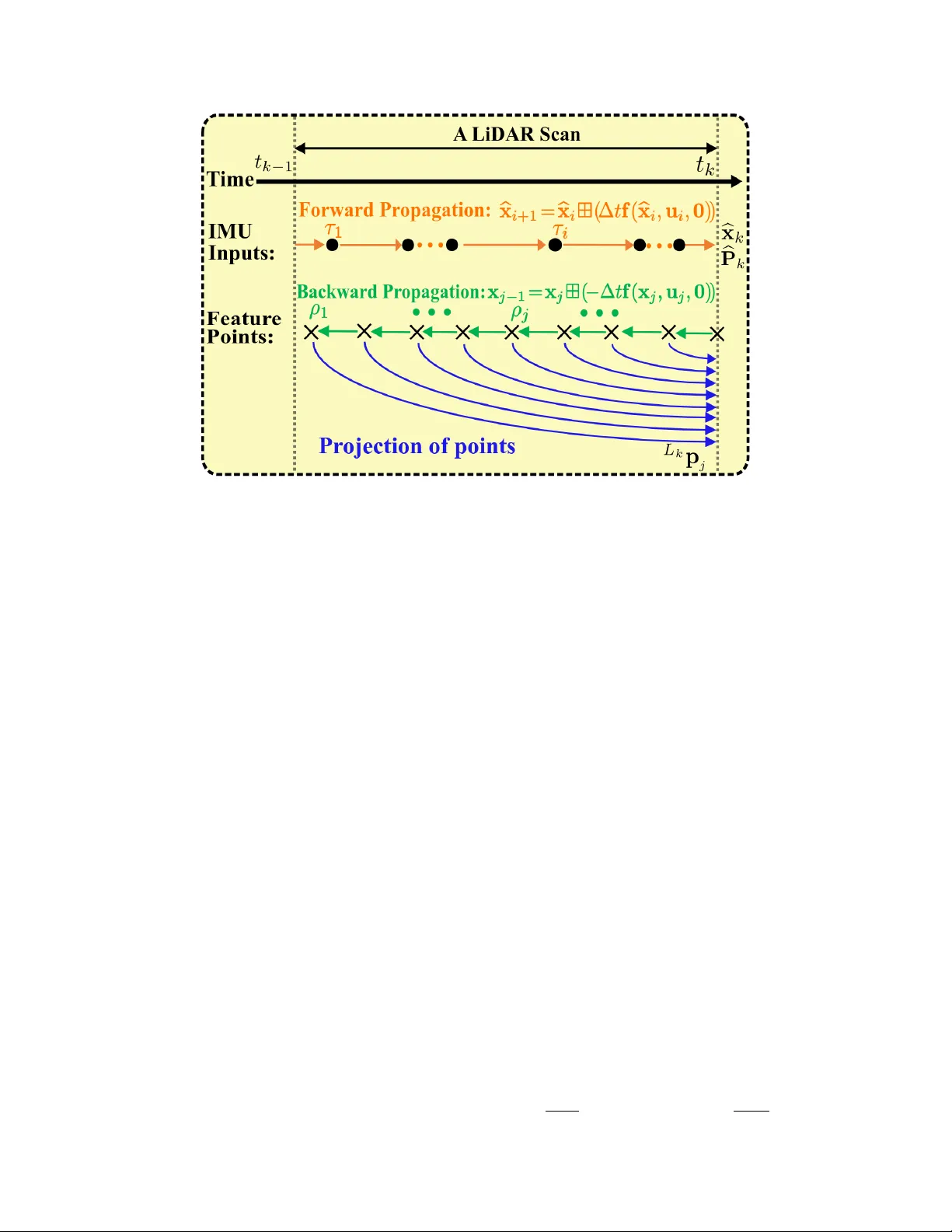
On the Deriv ation of Tigh tly-Coupled LiD AR-Inertial Odometry with V o xelMap Zhihao Zhan ∗ Abstract This note presen ts a concise mathematical formulation of tigh tly-coupled LiDAR-Inertial Odom- etry within an iterated error-state Kalman filter framew ork using a V o xelMap representation. Rather than prop osing a new algorithm, it provides a clear and self-contained deriv ation that unifies the geometric mo deling and probabilistic state estimation through consisten t notation and explicit form ulations. The do cumen t is intended to serv e b oth as a technical reference and as an accessible entry p oint for a foundational understanding of the system architecture and estimation principles. 1 In tro duction The rapid developmen t of 3D Light Detection and Ranging (LiD AR) technology has accelerated its adoption across diverse applications, including autonomous driving, rob otics, and large-scale en viron- men tal mapping [1–3]. Owing to its high geometric accuracy and robustness to illumination v ariations, LiD AR has b ecome a primary sensing mo dality for p erception and state estimation, driving significan t progress in LiDAR-based o dometry , particularly LiD AR–Inertial Odometry (LIO), which integrates inertial measurements for accurate and robust motion estimation. T o impro ve estimation robustness and consistency , mo dern LIO systems predominantly adopt tigh tly-coupled form ulations, where inertial and LiDAR measurements are join tly incorporated within a unified estimation framework [4–7]. By directly in tegrating geometric constraints into the filtering or optimization pro cess, tigh tly-coupled approac hes enable consistent uncertaint y propagation and stronger cross-mo dal coupling than lo osely-coupled strategies. Error-state Kalman filter (ESKF) and its iterative v ariants are therefore widely adopted due to their computational efficiency and suitability for real-time estimation [8]. In particular, the iterated extended Kalman filter (IEKF) further en- hances the ESKF framework by rep eatedly relinearizing nonlinear measuremen t mo dels around the latest estimate, making it esp ecially suitable for handling the strong nonlinearity of LiDAR geometric constrain ts [9]. In tightly-coupled LIO systems, the effectiveness of geometric constraints dep ends strongly on how the environmen t is represen ted during estimation. The map representation m ust preserv e lo cal struc- ture while supp orting efficient data asso ciation and incremental up dates under real-time constraints. T raditional feature-based or dense representations often struggle to balance accuracy and efficiency , motiv ating structured spatial representations. Among these, vo xel-based maps hav e gained increasing atten tion for organizing measurements into locally consistent regions while maintaining computational scalabilit y , making them well suited for tightly-coupled LIO systems [10–13]. Despite the rapid dev elopment of tigh tly-coupled LIO systems, their underlying form ulations are of- ten presented in implementation-orien ted forms, where geometric modeling and estimation pro cedures are describ ed separately or implicitly . As a result, the interaction b et ween probabilistic map repre- sen tation and state estimation is not alwa ys explicitly articulated. Motiv ated by this observ ation, this note provides a concise and self-contained mathematical deriv ation of V o xelMap-based tightly-coupled LIO with consistent notation and explicit formulation. ∗ Email: zhihazhan2-c@my .cityu.edu.hk 1 The remainder of this note is organized as follo ws. Section 2 introduces the system notation, op er- ators, and kinematic mo deling. Section 3 presents the probabilistic V oxelMap [10] represe n tation and its construction. Section 4 deriv es the tightly-coupled LIO formulation, including state propagation, motion comp ensation, geometric residual mo deling, and iterated Kalman up dates, following a pip eline consisten t with F AST-LIO2 [4]. Section 5 concludes the note. 2 Preliminaries This note adopts the notation summarized in T able 1. An o verview of the system w orkflo w is illustrated in Figure 1. LiD AR and inertial measuremen t unit (IMU) measurements are first pro cessed to obtain undistorted point clouds and propagated states. The preprocessed measuremen ts are then incorp orated in to an iterated error-state Kalman filter (IESKF) for state correc tion at the LiDAR rate (e.g., 10 Hz). The estimated p ose is used to register the LiDAR p oin ts to the global frame and up date the V o xelMap constructed so far. The up dated map subsequently serves as the reference for registering incoming measuremen ts. Figure 1: System ov erview of the V o xelMap-based LIO framew ork. LiD AR and IMU mea- suremen ts are prepro cessed and fused within an iterated error-state Kalman filter. The estimated p ose registers p oints to the global frame and incrementally up dates the V oxelMap. 2 T able 1: Imp ortant Notations. Sym b ols Meaning t k The scan-end time of the k -th LiDAR scan. τ i The i -th IMU sample time in a LiD AR scan. ρ j The j -th feature p oint’s sample time in a LiD AR scan. I i , I j , I k The IMU b o dy frame at the time τ i , ρ j and t k . L j , L k The LiDAR b o dy frame at the time ρ j and t k . x , b x , ¯ x The ground-true, propagated, and up dated v alue of x . e x The error b etw een ground-true x and its estimation ¯ x . b x κ The κ -th up date of x in the iterated Kalman filter. x i , x j , x k The vector (e.g.,state) x at time τ i , ρ j and t k . ˇ x j Estimate of x j relativ e to x k in the back propagation. 2.1 Op erator ⊞ / ⊟ F ollowing [4, 14], let M denote an n -dimensional manifold (e.g., M = SO (3)). Owing to the lo cal homeomorphism b etw een manifolds and R n , a lo cal bijection betw een M and its tangent space can be defined using the encapsulation op erators ⊞ and ⊟ ⊞ : M × R n → M , ⊟ : M × M → R n , M = SO (3) : R ⊞ r = R Exp ( r ) , R 1 ⊟ R 2 = Log  R T 2 R 1  , M = R n : a ⊞ b = a + b , a ⊟ b = a − b . (1) where Exp ( r ) = I + ⌊ r ⌋ ∧ ∥ r ∥ sin ( ∥ r ∥ ) + ⌊ r ⌋ 2 ∧ ∥ r ∥ 2 (1 − cos ( ∥ r ∥ )) is the exp onential map and Log( · ) is its inv erse map. F or a comp ound manifold M = SO (3) × R n w e ha ve  R a  ⊞  r b  =  R ⊞ r a + b  ,  R 1 a  ⊟  R 2 b  =  R 1 ⊟ R 2 a − b  . F rom the ab ov e definition, it is easy to verify that ( x ⊞ u ) ⊟ x = u , x ⊞ ( y ⊟ x ) = y , ∀ x , y ∈ M , ∀ u ∈ R n . 2.2 Kinematic Mo dels The evolution of the system state is gov erned by a kinematic mo del driven by inertial measurements. F or clarity of deriv ation, the dynamics are first form ulated in contin uous time to capture the under- lying motion. The mo del is then discretized ov er finite sampling interv als, yielding a discrete-time represen tation used in the subsequent estimation framework. 2.2.1 Con tinuous Mo del Assuming that the IMU is rigidly attached to the LiDAR with a known extrinsic I L T =  I L R , I L t  , we tak e the IMU frame (denoted as { I } ) as the b ody frame of reference. The global frame { G } is chosen to coincide with the initial IMU frame. This leads to the follo wing con tinuous-time kinematic mo del G I ˙ t = G I v , G I ˙ v = G I R ( a m − b a − n a ) + G g , G ˙ g = 0 , G I ˙ R = G I R ⌊ ω m − b ω − n ω ⌋ ∧ , ˙ b ω = n b ω , ˙ b a = n ba (2) where G I t , G I R are the p osition and attitude of IMU in the global frame { G } , G g is the gravit y vector expressed in { G } , a m and ω m are IMU measuremen ts, n a and n ω are zero-mean white Gaussian measuremen t noises, b a and b ω are IMU biases mo deled as random walks driven by Gaussian noises 3 n ba and n b ω , and the notation ⌊ a ⌋ ∧ denotes the skew-symmetric matrix of vector a ∈ R 3 that maps the cross pro duct op eration. The contin uous-time system dynamics in (2) are deriv ed from the follo wing IMU measurement mo del a m = G I R T  G a − G g  + b a + n a , ω m = ω + b ω + n ω , ˙ b ω = n b ω , ˙ b a = n ba (3) where G a denotes the true linear acceleration of the IMU expressed in the global frame, and ω is the true angular velocity expressed in the IMU frame. Based on the IMU measuremen t mo del in (3), the p osition dynamics follow directly from the definition of velocity , i.e., G I ˙ t = G I v . The v elocity dynamics are obtained by rewriting th e accelerometer measuremen t equation as b elo w. a m − b a − n a = G I R T  G a − G g  , → G a = G I R ( a m − b a − n a ) + G g . (4) Since the true linear acceleration in the global frame satisfies G a = G I ˙ v , substituting into the ab ov e expression yields G I ˙ v = G I R ( a m − b a − n a ) + G g . Similarly , the attitude kinematics on S O (3) are gov erned by G I ˙ R = G I R ⌊ ω ⌋ ∧ , where ω is the true angular velocity expressed in the IMU frame. Substituting the gyroscop e model in (3), giv es the con tinuous-time attitude dynamics G I ˙ R = G I R ⌊ ω m − b ω − n ω ⌋ ∧ . (5) The gravit y vector is assumed constan t in the global frame, i.e., G ˙ g = 0 . Moreo ver, the gyroscop e and accelerometer biases are mo deled as random w alks driven by white Gaussian noises, yielding ˙ b ω = n b ω , ˙ b a = n ba . 2.2.2 Discrete Model By in tegrating the con tinuous-time kinematics o v er a sampling in terv al ∆ t , the follo wing exact integral form is obtained G I R ( t + ∆ t ) = G I R ( t ) Exp Z t+∆t t ω ( τ ) d τ ! , G I v ( t + ∆ t ) = G I v ( t ) + Z t +∆ t t G a ( τ ) dτ , G I t ( t + ∆ t ) = G I t ( t ) + Z t +∆ t t G I v ( τ ) dτ . (6) Starting from (6), a discrete-time mo del is obtained by assuming that the angular velocity and acceleration are approximately constan t within each sampling in terv al [ t i , t i +1 ] with t i +1 = t i + ∆ t . Using a first-order appro ximation for the integrals yields G I i +1 R = G I i R Exp ( ω i ∆t) , G I i +1 v = G I i v + G a i ∆ t, G I i +1 t = G I i t + G I i v ∆ t (7) where G I i R ≜ G I R ( t i ), G I i v ≜ G I v ( t i ), and G I i t ≜ G I t ( t i ). Substituting the IMU measurement mo del in (3), gives the following discrete mo del G I i +1 R = G I i R Exp (( ω m i − b ω i − n ω i ) ∆t) , G I i +1 v = G I i v +  G I i R ( a m i − b a i − n a i ) + G g i  ∆ t, G I i +1 t = G I i t + G I i v ∆ t. (8) 4 Based on the ⊞ op eration and discrete-time model in (8) defined ab o ve, w e can discretize the con tinuous mo del in (2) at the IMU sampling pe riod ∆ t . The resultant discrete mo del is x i +1 = x i ⊞ (∆ t f ( x i , u i , w i )) (9) where i is the index of IMU measurements, the function f , state x , input u and noise w are defined as b elow M = S O (3) × R 15 , dim( M ) = 18 , x . =  G I R T G I t T G I v T b T ω b T a G g T  T ∈ M , u . =  ω T m a T m  T , w . =  n T ω n T a n T b ω n T ba  T , f ( x i , u i , w i ) =         ω m i − b ω i − n ω i , G I i v G I i R ( a m i − b a i − n a i ) + G g i n b ω i n ba i 0 3 × 1         . (10) 3 Probabilistic V o xelMap Represen tation 3.1 Probabilistic Plane Represen tation F ollowing the probabilistic V o xelMap form ulation in [10], eac h vo xel main tains a single probabilistic plane feature to represent lo cal geometry . Since a plane is estimated from its asso ciated LiDAR p oin ts, its uncertaint y is determined b y the uncertainties of those p oints. As V o xelMap is expressed in the global frame, the uncertaint y of point G p i m ust b e analyzed after transformation from the lo cal LiD AR frame, leading to tw o principal noise sources: raw measuremen t noise and uncertaint y of p ose estimation. The follo wing subsections deriv e the corres ponding uncertaint y propagation from p oin ts to planes and establish the probabilistic plane represen tation. 3.1.1 Uncertain ty of p oin t G p i F ollowing the LiD AR measurement noise analysis in [15], the uncertain ty of a point in the lo cal LiD AR frame is mo deled as the combination of ranging noise and bearing direction noise as shown in Figure 2. Let ϕ ∈ S 2 denote the measured b earing direction with p erturbation δ ϕ i ∼ N ( 0 2 × 1 , Σ ϕ i ) defined on its tangent plane, and let d i b e the measured depth with ranging noise δ d i ∼ N (0 , Σ d i ). Figure 2: The uncertain ty mo del of the registered p oint. Using the ⊞ operation encapsulated in S 2 [16], define the relation betw een the true bearing direction ϕ g t i and its measurement ϕ i as b elow ϕ g t i = ϕ i ⊞ S 2 δ ϕ i ≜ Exp ( N ( ϕ i ) δ ϕ i ) ϕ i ≈ ( I + ⌊ N ( ϕ i ) δ ϕ i ⌋ ∧ ) ϕ i (11) 5 where N ( ϕ i ) =  N 1 N 2  ∈ R 3 × 2 is an orthonormal basis of the tangent plane at ϕ i (see Figure 2). The ⊞ S 2 op eration essentially rotates the unit v ector ϕ i ab out the axis δ ϕ i in the tangen t plane at ϕ i , the result is still a unit vector (i.e., remain on S 2 ). Similarly , the ground-truth depth d g t i can b e expressed b elow d g t i = d i + δ d i . (12) Com bining (11) and (12), we can obtain the relation b etw een the ground-truth p oin t L p g t i and its measuremen t L p i L p g t i = d g t i ϕ g t i = ( d i + δ d i ) ( ϕ i ⊞ S 2 δ ϕ i ) ≈ ( d i + δ d i ) ( ϕ i + ⌊ N ( ϕ i ) δ ϕ i ⌋ ∧ ϕ i ) = d i ϕ i + ϕ i δ d i + d i ⌊ N ( ϕ i ) δ ϕ i ⌋ ∧ ϕ i + O ( δ d i δ ϕ i ) ≈ d i ϕ i + ϕ i δ d i − d i ⌊ ϕ i ⌋ ∧ N ( ϕ i ) δ ϕ i = L p i + δ L p i (13) where L p i ≜ d i ϕ i , and δ L p i ≜ ϕ i δ d i − d i ⌊ ϕ i ⌋ ∧ N ( ϕ i ) δ ϕ i . T o get the formulation in [10, 15], rewrite δ L p i as shown δ L p i = ϕ i δ d i − d i ⌊ ϕ i ⌋ ∧ N ( ϕ i ) δ ϕ i =  ϕ i − d i ⌊ ϕ i ⌋ ∧ N ( ϕ i )   δ d i δ ϕ i  . (14) W e can let A i =  ϕ i − d i ⌊ ϕ i ⌋ ∧ N ( ϕ i )  ∈ R 3 × 3 , thus δ L p i ∼ N  0 , Σ L p i  , Σ L p i = A i  Σ d i 0 1 × 2 0 2 × 1 Σ ϕ i  A T i =  ϕ i − d i ⌊ ϕ i ⌋ ∧ N ( ϕ i )   Σ d i 0 1 × 2 0 2 × 1 Σ ϕ i   ϕ T i − d i ( ⌊ ϕ i ⌋ ∧ N ( ϕ i )) T  = ϕ i Σ d i ϕ T i + d 2 i ⌊ ϕ i ⌋ ∧ N ( ϕ i ) Σ ϕ i N ( ϕ i ) T ⌊ ϕ i ⌋ T ∧ . (15) Considering that the LiDAR p oint L p i will be further pro jected to the world frame through the estimated p ose G L T =  G L R , G L t  ∈ SE (3), with estimation uncertaint y ( Σ R , Σ t ), by the follo wing rigid transformation G p i = G L R L p i + G L t . (16) Therefore, the uncertaint y of the LiDAR p oints G p i can b e obtained by G p g t i = G L R g t L p g t i + G L t g t = G L R Exp ( δ θ )  L p i + δ L p i  + G L t + δ t ≈ G L R ( I + ⌊ δ θ ⌋ ∧ )  L p i + δ L p i  + G L t + δ t = G L R L p i + G L R δ L p i + G L R ⌊ δ θ ⌋ ∧ L p i + O  δ θ , δ L p i  + G L t + δ t ≈ G p i + G L R δ L p i − G L R ⌊ L p i ⌋ ∧ δ θ + δ t , δ G p i = G L R δ L p i − G L R ⌊ L p i ⌋ ∧ δ θ + δ t ∼ N  0 , Σ G p i  , Σ G p i = Σ t + G L RΣ L p i G L R T + G L R ⌊ L p i ⌋ ∧ Σ R  G L R ⌊ L p i ⌋ ∧  T = G L RΣ L p i G L R T + G L R ⌊ L p i ⌋ ∧ Σ R ⌊ L p i ⌋ T ∧ G L R T + Σ t (17) where δ θ ∈ R 3 and δ t ∈ R 3 denote the small p erturbations of the rotation and translation components of the estimated pose, resp ectiv ely . 6 3.1.2 Uncertain ty of plane Referring to [10, 17], let a plane feature consist of a group of LiDAR p oints G p i ( i = 1 , . . . , N ), each has an uncertaint y Σ G p i due to the measurement noise and p ose estimation error as shown in (17). Denote the centroid and cov ariance matrix of the p oints b y ¯ p and A , resp ectiv ely ¯ p = 1 N N X i =1 G p i , A = 1 N N X i =1  G p i − ¯ p   G p i − ¯ p  T . (18) Then, the plane can b e represen ted b y its normal v ector n , which is the eigenv ector asso ciated with the minim um eigenv alue of A , and the point q = ¯ p , which lies in this plane. As b oth A and q are dep enden t on G p i , denote the plane parameters ( n , q ) as functions of G p i  n , q  T = f  G p 1 , G p 2 , . . . , G p N  . (19) Figure 3: The Uncertain ty mo del of the plane normal. Next, we deriv e the uncertaint y of plane shown in Figure 3 based on the uncertaint y of p oin t G p i in (17). The ground-truth normal vector n g t and ground-truth p osition q g t are  n g t , q g t  T = f  G p 1 + δ G p 1 , G p 2 + δ G p 2 , . . . , G p N + δ G p N  ≈  n , q  T + N X i =1 ∂ f ∂ G p i δ G p i , δ n , q = N X i =1 ∂ f ∂ G p i δ G p i ∼ N ( 0 , Σ n , q ) (20) where ∂ f ∂ G p i = h ∂ n ∂ G p i , ∂ q ∂ G p i i T . Thus, w e can get the uncertaint y of the plane Σ n , q = P N i =1 ∂ f ∂ G p i Σ G p i ∂ f ∂ G p i T . According to (18), w e can easily take the deriv ativ e of q with resp ect to each p oint G p i ∂ q ∂ G p i = 1 N I 3 . (21) Then, do the the deriv ativ e of n with resp ect to eac h p oint G p i . The normal vector n is the eigen vector asso ciated with the minimum eigen v alue λ 3 of A m en tioned in (18). Also, we hav e the definition of eigenv ector and eigenv alue U =  u 1 u 2 u 3  , Λ =   λ 1 0 0 0 λ 2 0 0 0 λ 3   , U T U = I , A = UΛU T , Λ = U T A U , A U = UΛ , U T A = ΛU T . (22) 7 T ake the deriv ativ e of U T U with resp ect to each p oint G p i U T ∂ U ∂ G p i + ∂ U ∂ G p i T U = 0 , Let C p i = U T ∂ U ∂ G p i , → C p i + C p i T = 0 (23) where C p i is a sk ew-symmetric matrix whose diagonal elements are zeros. Using (23), take the deriv ativ e of Λ with resp ect to each p oint G p i ∂ Λ ∂ G p i = ∂ U T ∂ G p i A U + U T ∂ A ∂ G p i U + U T A ∂ U ∂ G p i = U T ∂ A ∂ G p i U + ΛU T ∂ U ∂ G p i + ∂ U T ∂ G p i UΛ = U T ∂ A ∂ G p i U + ΛC p i − C p i Λ . (24) Since Λ is diagonal, ∂ Λ ∂ G p i , for off-diagonal elemen t in (24), we ha ve 0 = u T m ∂ A ∂ G p i u n + λ m C p i m,n − C p i m,n λ n , → u T m ∂ A ∂ G p i u n = ( λ n − λ m ) C p i m,n , → C p i m,n = 1 λ n − λ m u T m ∂ A ∂ G p i u n , m  = n (25) where C p i m,n is the m -th ro w and n -th column element in C p i . Using (23) and (25), gives C p i m,n =    1 λ n − λ m u T m ∂ A ∂ G p i u n , m  = n 0 1 × 3 , m = n (26) According to the form ulation of C p i in (23), yield ∂ U ∂ G p i = UC p i = UU T ∂ U ∂ G p i . (27) Using e k , a 3 × 1 vector in whic h the k -th element is 1 and the rests 0, combined with (27), gives ∂ u k ∂ G p i = ∂ U ∂ G p i e k , Let G p i =  x i y i z i  , → ∂ u k ∂ G p i = h ∂ U ∂ x i e k ∂ U ∂ y i e k ∂ U ∂ z i e k i =  UC x i e k UC y i e k UC z i e k  = U  C x i e k C y i e k C z i e k  = U   C x i 1 ,k C y i 1 ,k C z i 1 ,k C x i 2 ,k C y i 2 ,k C z i 2 ,k C x i 3 ,k C y i 3 ,k C z i 3 ,k   (28) where C x i ≜ U T ∂ U ∂ x i ∈ R 3 × 3 , C y i ≜ U T ∂ U ∂ y i ∈ R 3 × 3 and C z i ≜ U T ∂ U ∂ z i ∈ R 3 × 3 . T o simplify (28), define F p i m,n =  C x i m,n C y i m,n C z i m,n  ∈ R 1 × 3 , m, n ∈ { 1 , 2 , 3 } ∂ u k ∂ G p i = U   F p i 1 ,k F p i 2 ,k F p i 3 ,k   = UF p i k . (29) 8 So far, only F p i m,n has not b een fully deriv ed. According to (26), hence F p i m,n =      1 λ n − λ m ∂ u T m Au n ∂ G p i , m  = n 0 1 × 3 , m = n (30) T o further obtain the sp ecific form of F p i m,n , derive ∂ u T m Au n ∂ G p i ( u m and u n are viewed as constan t vector) ∂ u T m Au n ∂ G p i = 1 N N X j =1 ∂ u T m  G p j − ¯ p   G p j − ¯ p  T u n ∂ G p i = 1 N N X j =1 ∂ u T m  G p j − ¯ p  u T n  G p j − ¯ p  ∂ G p i , Let e j = u T m  G p j − ¯ p  ∈ R , f j = u T n  G p j − ¯ p  ∈ R , → ∂ u T m Au n ∂ G p i = 1 N N X j =1 ∂ e j f j ∂ G p i = 1 N N X j =1 e j ∂ f j ∂ G p i + f j ∂ e j ∂ G p i . (31) Then, N X j =1 e j ∂ f j ∂ G p i = N X j =1 u T m  G p j − ¯ p  ∂ u T n  G p j − ¯ p  ∂ G p i = u T m  G p i − ¯ p  ∂ u T n  G p i − ¯ p  ∂ G p i + N X j =1 ,j  = i u T m  G p j − ¯ p  ∂ u T n  G p j − ¯ p  ∂ G p i =  G p i − ¯ p  T u m u T n (1 − 1 N ) + N X j =1 ,j  = i  G p j − ¯ p  T u m u T n ( − 1 N ) =  G p i − ¯ p  T u m u T n (1 − 1 N ) +  G p i − ¯ p  T u m u T n 1 N =  G p i − ¯ p  T u m u T n . (32) Similarly , derive that P N j =1 f j ∂ e j ∂ G p i =  G p i − ¯ p  T u n u T m . Using (31) and (32), we can directly giv e ∂ u T m Au n ∂ G p i =  G p i − ¯ p  T  u m u T n + u n u T m  when m  = n . Also, F p i m,n =       G p i − ¯ p  T N ( λ n − λ m )  u m u T n + u n u T m  , m  = n 0 1 × 3 , m = n (33) Refer to (29) and (33), rec all that the normal vector n is the eigenv ector asso ciated with the minimum eigen v alue λ 3 of A ∂ n ∂ G p i = U   F p i 1 , 3 F p i 2 , 3 F p i 3 , 3   , F p i m, 3 =       G p i − ¯ p  T N ( λ 3 − λ m )  u m n T + nu T m  , m  = 3 0 1 × 3 , m = 3 (34) 9 Finally , give the uncertaint y of plane Σ n , q = N X i =1 ∂ f ∂ G p i Σ G p i ∂ f ∂ G p i T = N X i =1 " ∂ n ∂ G p i ∂ q ∂ G p i # Σ G p i h ∂ n ∂ G p i T ∂ q ∂ G p i T i = N X i =1 " ∂ n ∂ G p i Σ G p i ∂ n ∂ G p i T ∂ n ∂ G p i Σ G p i ∂ q ∂ G p i T ∂ q ∂ G p i Σ G p i ∂ n ∂ G p i T ∂ q ∂ G p i Σ G p i ∂ q ∂ G p i T # . (35) 3.2 Map Construction and Up date Referring to [10], a coarse-to-fine v oxel mapping metho d was proposed, whic h can build a rough v oxel map when the p oint cloud is sparse and refine the map when more points are receiv ed. Since LiD AR p oints are acquired sequen tially , each scan is initially sparse, esp ecially in large-scale outdo or en vironments. Under such conditions, conv entional fine-to-coarse surfel mapping often yields to o few reliable planes, motiv ating the coarse-to-fine V o xelMap strategy to improv e plane construction from sparse observ ations while reducing reliance on long accumulation in terv als. T o construct the V o xelMap in a coarse-to-fine manner, the global space is first partitioned into coarse vo xels, which are indexed b y a hash table. Each occupied v oxel is further represented by an o ctree, where plane fitting is recursiv ely p erformed on the contained p oin ts. If the p oin ts within a v oxel satisfy a planar criterion, the plane parameters and their uncertaint y are estimated and stored; otherwise, the vo xel is sub divided into eigh t c hild v oxels until a v alid plane is found or the maximum o ctree depth is reac hed. In this w ay , v oxels of differen t sizes are adaptiv ely generated, eac h main taining a single probabilistic plane feature fitted from its raw LiD AR p oints. F or online op eration, newly registered LiD AR p oints are contin uously inserted into the V oxelMap according to the estimated p ose as shown in Figure 1. If a p oint falls into an uno ccupied region, a new v oxel is created; otherwise, the corresp onding plane parameters and uncertain ty are up dated. T o limit the computational growth caused b y accumulating historical p oin ts, the up date process exploits the empirical conv ergence of plane uncertaint y . Once the plane estimate b ecomes sufficien tly stable, historical p oints are discarded and only the plane parameters, cov ariance, and a small set of recent p oin ts are retained. If the normal vector estimated from newly arriving p oints deviates significan tly from the stored plane, the vo xel is regarded as changed and is reconstructed. 4 Error-State Kalman Filter for LiD AR-Inertial Odometry This section presents the tigh tly-coupled LiD AR-Inertial Odometry formulation under the error-state Kalman filter framew ork. F ollowing the system mo del in tro duced in Section 2 and the probabilistic V oxelMap representation established in Section 3, the complete estimation pip eline is formulated, including IMU forward propagation, backw ard propagation for motion comp ensation, p oin t-to-plane residual construction, and the iterated Kalman up date. T o estimate the states in the state formulation (10), use an iterated extended Kalman filter like [4]. Assume the optimal state estimate of the last LiDAR scan at t k − 1 is ¯ x k − 1 with cov ariance matrix ¯ P k − 1 . Then ¯ P k − 1 represen ts the cov ariance of the random error state vector defined b elo w: e x k − 1 . = x k − 1 ⊟ ¯ x k − 1 = h δ θ T G I e t T G I e v T e b T ω e b T a G e g T i T (36) where δ θ = Log  G I ¯ R T G I R  is the attitude error and the rest are standard additive errors (i.e., the error in the estimate ¯ x of a quantit y x is e x = x − ¯ x ). In tuitively , the attitude error δ θ describes the (small) deviation b et ween the true and estimated attitude. The main adv antage of this error definition is that it allows us to represen t the uncertaint y of attitude b y the 3 × 3 co v ariance matrix E { δ θ δ θ T } . Since the attitude has 3 degree of freedom (DOF), this is a minimal representation. 10 Figure 4: The forw ard and bac kward propagation. 4.1 IMU F orw ard Propagation The forw ard propagation is p erformed up on receiving each IMU measurement (see Figure 4). Sp ecifi- cally , the state is propagated following (9) by setting the pro cess noise w i to zero b x i +1 = b x i ⊞ (∆ t f ( b x i , u i , 0 )) ; b x 0 = ¯ x k − 1 (37) where ∆ t = τ i +1 − τ i . T o propagate the cov ariance, we use the error state dynamic mo del obtained b elo w e x i +1 = x i +1 ⊟ b x i +1 = ( x i ⊞ ∆ t f ( x i , u i , w i )) ⊟ ( b x i ⊞ ∆ t f ( b x i , u i , 0 )) ≈ F e x e x i + F w w i (38) where the matrices F e x and F w are derived b elow. Denoting the co v ariance of white noises w as Q , then the propagated co v ariance b P i can b e computed recursively as b P i +1 = F e x b P i F T e x + F w QF T w ; b P 0 = ¯ P k − 1 . (39) The propagation contin ues until the end time of a new scan at t k where the propagated state and co v ariance are denoted as b x k , b P k . Thus, b P k represen ts the cov ariance of the propagation error x k ⊟ b x k . Here, tw o equiv alent deriv ations of F e x and F w are considered: (i) direct first-order T a ylor linearization of the discrete propagation, and (ii) deriv ation of the con tinuous-time error dynamics ˙ e x follo wed b y discretization. 4.1.1 Metho d 1: Direct Discrete-time Linearization First, consider a general discrete-time nonlinear system using first-order T a ylor linearization x i = f ( x i − 1 , u i − 1 , w i − 1 ) , → b x i ⊞ e x i = f ( b x i − 1 ⊞ e x i − 1 , u i − 1 , w i − 1 ) ≈ f ( b x i − 1 , u i − 1 , 0 ) + F e x i − 1 + Gw i − 1 (40) where u i − 1 and w i − 1 denote the input and pro cess noise, F ≜ ∂ f ∂ x i − 1    ( b x i − 1 , u i − 1 , 0 ) and G ≜ ∂ f ∂ w i − 1    ( b x i − 1 , u i − 1 , 0 ) . 11 Let g ( e x i , w i ) ≜ ∆ t f ( x i , u i , w i ) = ∆ t f ( b x i ⊞ e x i , u i , w i ), thus (38) can b e rewritten as e x i +1 = ( x i ⊞ ∆ t f ( x i , u i , w i )) ⊟ ( b x i ⊞ ∆ t f ( b x i , u i , 0 )) = (( b x i ⊞ e x i ) ⊞ g ( e x i , w i )) ⊟ ( b x i ⊞ g ( 0 , 0 )) ≜ G ( e x i , g ( e x i , w i )) . (41) F ollowing (40), linearize the state mo del at e x i = 0 and w i = 0 F e x = ∂ G ( e x i , g ( 0 , 0 )) ∂ e x i + ∂ G ( 0 , g ( e x i , 0 )) ∂ g ( e x i , 0 ) ∂ g ( e x i , 0 ) ∂ e x i     e x i = 0 , F w = ∂ G ( 0 , g ( 0 , w i )) ∂ g ( 0 , w i ) ∂ g ( 0 , w i ) ∂ w i     w i = 0 . (42) F or manifold-v alued expressions of the form E = (( a ⊞ b ) ⊞ c ) ⊟ d , the required Jacobians are ev aluated using the differential rules of the ⊞ / ⊟ calculus on manifolds ∂ E ∂ b = ∂ E ∂ c = I n × n , a , b , c , d ∈ R n . (43) Sp ecifically for b , c ∈ R 3 , a , d ∈ SO (3), the Jacobians are different. ∂ E ∂ b is derived as E = (( a ⊞ b ) ⊞ c ) ⊟ d = Log  d T ( a ⊞ b ) ⊞ c  , → Exp ( E ) = d T a Exp ( b ) Exp ( c ) , → Exp ( E + δ E ) = d T a Exp ( b + δ b ) Exp ( c ) , B C H → Exp ( E ) Exp  J l ( E ) T δ E  = d T a Exp ( b ) Exp  J l ( b ) T δ b  Exp ( c ) , → Exp  J l ( E ) T δ E  = Exp ( c ) T Exp  J l ( b ) T δ b  Exp ( c ) Adjoin t 1 = Exp  Exp ( c ) T J l ( b ) T δ b  , → J l ( E ) T δ E = Exp ( − c ) J l ( b ) T δ b , → ∂ E ∂ b = J l ( E ) − T Exp ( − c ) J l ( b ) T (44) where J l ( u ) = sin θ θ I +  1 − sin θ θ  aa T + 1 − cos θ θ ⌊ a ⌋ ∧ , u = θ a , ∥ a ∥ = 1 and Adjoin t 1 represents R Exp ( p ) R T = Exp ( Rp ) , R ∈ SO (3) , p ∈ R 3 . ∂ E ∂ c is similarly derived to Exp ( E + δ E ) = d T a Exp ( b ) Exp ( c + δ c ) , B C H → Exp ( E ) Exp  J l ( E ) T δ E  = d T a Exp ( b ) Exp ( c ) Exp  J l ( c ) T δ c  , → Exp  J l ( E ) T δ E  = Exp  J l ( c ) T δ c  , → J l ( E ) T δ E = J l ( c ) T δ c , → ∂ E ∂ c = J l ( E ) − T J l ( c ) T . (45) Referring to (43) and (44), ∂ G ( e x i , g ( 0 , 0 )) ∂ e x i     e x i = 0 =  J l ( 0 ) − 1 Exp ( − g ( 0 , 0 )) J l ( 0 ) T 0 0 I 15 × 15  =  Exp ( − ∆t f ( b x i , u i , 0 )) 0 0 I 15 × 15  = " Exp  − ∆t  ω m i − b b ω i  0 0 I 15 × 15 # . (46) 12 Referring to (43) and (45), ∂ G ( 0 , g ( e x i , 0 )) ∂ g ( e x i , 0 )     e x i = 0 =  J l ( 0 ) − 1 J l ( g ( 0 , 0 )) T 0 0 I 15 × 15  = " J l  ∆ t  ω m i − b b ω i  T 0 0 I 15 × 15 # . (47) As g ( e x i , w i ) = ∆ t f ( b x i ⊞ e x i , u i , w i ), thus g ( e x i , w i ) = ∆ t         ω m i − b ω i − n ω i G I i v G I i R ( a m i − b a i − n a i ) + G g i n b ω i n ba i 0 3 × 1         = ∆ t          ω m i − b b ω i − e b ω i − n ω i G I i b v + G I i e v G I i b R Exp ( δ θ i )  a m i − b b a i − e b a i − n a i  + G g i n b ω i n ba i 0 3 × 1          , → g ( e x i , 0 ) = ∆ t          ω m i − b b ω i − e b ω i G I i b v + G I i e v G I i b R Exp ( δ θ i )  a m i − b b a i − e b a i  + G g i 0 3 × 1 0 3 × 1 0 3 × 1          = ∆ t          ω m i − b b ω i − e b ω i G I i b v + G I i e v G I i b R  a m i − b b a i − e b a i  − G I i b R ⌊ a m i − b b a i − e b a i ⌋ ∧ δ θ i + G g i 0 3 × 1 0 3 × 1 0 3 × 1          , → ∂ g ( e x i , 0 ) ∂ e x i     e x i = 0 =         0 0 0 − I 3 × 3 ∆ t 0 0 0 0 I 3 × 3 ∆ t 0 0 0 − G I i b R ⌊ a m i − b b a i ⌋ ∧ ∆ t 0 0 0 − G I i b R ∆ t I 3 × 3 ∆ t 0 0 0 0 0 0 0 0 0 0 0 0 0 0 0 0 0 0         . (48) 13 Referring to (46), (47) and (48), we can derive the exact formulation of F e x F e x = ∂ G ( e x i , g ( 0 , 0 )) ∂ e x i + ∂ G ( 0 , g ( e x i , 0 )) ∂ g ( e x i , 0 ) ∂ g ( e x i , 0 ) ∂ e x i     e x i = 0 = " Exp  − ∆t  ω m i − b b ω i  0 0 I 15 × 15 # + " J l  ∆ t  ω m i − b b ω i  T 0 0 I 15 × 15 #         0 0 0 − I 3 × 3 ∆ t 0 0 0 0 I 3 × 3 ∆ t 0 0 0 − G I i b R ⌊ a m i − b b a i ⌋ ∧ ∆ t 0 0 0 − G I i b R ∆ t I 3 × 3 ∆ t 0 0 0 0 0 0 0 0 0 0 0 0 0 0 0 0 0 0         =          Exp  − ∆t  ω m i − b b ω i  0 0 −J l  ∆ t  ω m i − b b ω i  T ∆ t 0 0 0 I 3 × 3 I 3 × 3 ∆ t 0 0 0 − G I i b R ⌊ a m i − b b a i ⌋ ∧ ∆ t 0 I 3 × 3 0 − G I i b R ∆ t I 3 × 3 ∆ t 0 0 0 I 3 × 3 0 0 0 0 0 0 I 3 × 3 0 0 0 0 0 0 I 3 × 3          ≈          Exp  − ∆t  ω m i − b b ω i  0 0 − I 3 × 3 ∆ t 0 0 0 I 3 × 3 I 3 × 3 ∆ t 0 0 0 − G I i b R ⌊ a m i − b b a i ⌋ ∧ ∆ t 0 I 3 × 3 0 − G I i b R ∆ t I 3 × 3 ∆ t 0 0 0 I 3 × 3 0 0 0 0 0 0 I 3 × 3 0 0 0 0 0 0 I 3 × 3          . (49) Similarly referring to (43) and (45), ∂ G ( 0 , g ( 0 , w i )) ∂ g ( 0 , w i )     w i = 0 =  J l ( 0 ) − 1 J l ( g ( 0 , 0 )) T 0 0 I 15 × 15  = " J l  ∆ t  ω m i − b b ω i  T 0 0 I 15 × 15 # . (50) Lik e (48), g ( 0 , w i ) = ∆ t          ω m i − b b ω i − n ω i G I i b v G I i b R  a m i − b b a i − n a i  + G b g i n b ω i n ba i 0 3 × 1          , ∂ g ( 0 , w i ) ∂ w i     w i = 0 =         − I 3 × 3 ∆ t 0 0 0 0 0 0 0 0 − G I i b R ∆ t 0 0 0 0 I 3 × 3 ∆ t 0 0 0 0 I 3 × 3 ∆ t 0 0 0 0         . (51) 14 Com bine (50) with (51), derive F w F w = " J l  ∆ t  ω m i − b b ω i  T 0 0 I 15 × 15 #         − I 3 × 3 ∆ t 0 0 0 0 0 0 0 0 − G I i b R ∆ t 0 0 0 0 I 3 × 3 ∆ t 0 0 0 0 I 3 × 3 ∆ t 0 0 0 0         =          −J l  ∆ t  ω m i − b b ω i  T ∆ t 0 0 0 0 0 0 0 0 − G I i b R ∆ t 0 0 0 0 I 3 × 3 ∆ t 0 0 0 0 I 3 × 3 ∆ t 0 0 0 0          ≈         − I 3 × 3 ∆ t 0 0 0 0 0 0 0 0 − G I i b R ∆ t 0 0 0 0 I 3 × 3 ∆ t 0 0 0 0 I 3 × 3 ∆ t 0 0 0 0         . (52) 4.1.2 Metho d 2: Contin uous-time Error Dynami cs and Discretization According to (2) and (36), we can easily derive the dynamics of δ t , δ b ω , δ b a and δ G g δ G I ˙ t = δ G I v , δ G ˙ g = 0 , δ ˙ b ω = n b ω , δ ˙ b a = n ba . (53) F or the dynamic of δ θ , G I ˙ R = G I R ⌊ ω m − b ω − n ω ⌋ ∧ , G I ˙ b R = G I b R ⌊ ω m − b b ω ⌋ ∧ , G I R = G I b R Exp ( δ θ ) , → G I ˙ R = G I ˙ b R Exp ( δ θ ) + G I b R Exp ( δ θ ) ⌊ δ ˙ θ ⌋ ∧ , → G I b R Exp ( δ θ ) ⌊ ω m − b ω − n ω ⌋ ∧ = G I b R ⌊ ω m − b b ω ⌋ ∧ Exp ( δ θ ) + G I b R Exp ( δ θ ) ⌊ δ ˙ θ ⌋ ∧ , → Exp ( δ θ ) ⌊ ω m − b ω − n ω ⌋ ∧ = ⌊ ω m − b b ω ⌋ ∧ Exp ( δ θ ) + Exp ( δ θ ) ⌊ δ ˙ θ ⌋ ∧ , → Exp ( δ θ ) ⌊ δ ˙ θ ⌋ ∧ = Exp ( δ θ ) ⌊ ω m − b ω − n ω ⌋ ∧ − ⌊ ω m − b b ω ⌋ ∧ Exp ( δ θ ) Adjoin t 2 = Exp ( δ θ ) ⌊ ω m − b ω − n ω ⌋ ∧ − Exp ( δ θ ) ⌊ Exp ( − δ θ )  ω m − b b ω  ⌋ ∧ , → δ ˙ θ = ( ω m − b ω − n ω ) − Exp ( − δ θ )  ω m − b b ω  ≈ ω m − b b ω − e b ω − n ω − ( I − ⌊ δ θ ⌋ ∧ )  ω m − b b ω  = −⌊ ω m − b b ω ⌋ ∧ δ θ − e b ω − n ω (54) 15 where Adjoint 2 denotes ⌊ p ⌋ ∧ R = R ⌊ R T p ⌋ ∧ , R ∈ SO (3) , p ∈ R 3 . F or the dynamic of δ G I ˙ v , G I ˙ v = G I R ( a m − b a − n a ) + G g , G I ˙ b v = G I b R  a m − b b a  + G b g , G I v = G I b v + G I e v , → G I ˙ v = G I ˙ b v + G I ˙ e v , → G I R ( a m − b a − n a ) + G g = G I b R  a m − b b a  + G b g + G I ˙ e v , G I ˙ e v = G I b R ( I + ⌊ δ θ ⌋ ∧ ) ( a m − b a − n a ) + G g − G I b R  a m − b b a  − G b g = G I b R  −⌊ a m − b a − n a ⌋ ∧ δ θ − e b a − n a  + G e g ≈ − G I b R ⌊ a m − b b a ⌋ ∧ δ θ − G I b R e b a − G I b Rn a + G e g . (55) T ake the discretization for contin uous-time error dynamics, δ θ i +1 = Exp  −  ω m i − b b ω i  ∆t  δ θ i − e b ω i ∆t − n ω i ∆t , G I i +1 e t = G I i e t + G I i e v ∆ t, G I i +1 e v = G I i e v +  − G I i b R ⌊ a m i − b b a i ⌋ ∧ δ θ i − G I i b R e b a i − G I i b Rn a i + G e g i  ∆ t, e b ω i +1 = e b ω i + n b ω i ∆ t, e b a i +1 = e b a i + n ba i ∆ t, G e g i +1 = G e g i . (56) Recall the error state mo del in (38), F e x =          Exp  −  ω m i − b b ω i  ∆t  0 0 − I 3 × 3 ∆ t 0 0 0 I 3 × 3 I 3 × 3 ∆ t 0 0 0 − G I i b R ⌊ a m i − b b a i ⌋ ∧ ∆ t 0 I 3 × 3 0 − G I i b R ∆ t I 3 × 3 ∆ t 0 0 0 I 3 × 3 0 0 0 0 0 0 I 3 × 3 0 0 0 0 0 0 I 3 × 3          , F w =         − I 3 × 3 ∆ t 0 0 0 0 0 0 0 0 − G I i b R ∆ t 0 0 0 0 I 3 × 3 ∆ t 0 0 0 0 I 3 × 3 ∆ t 0 0 0 0         . (57) 4.2 Bac kw ard Propagation for Motion Comp ensation Because LiD AR p oin ts within a scan are sampled at differen t time instan ts ρ j ≤ t k , directly associ- ating them with the scan-end state in tro duces motion distortion. T o comp ensate for this effect, the propagated state at the scan-end time t k is taken as the reference, and the relative motion from each p oin t timestamp ρ j bac k to t k is recov ered b y backw ard propagation ( ˇ x j − 1 = ˇ x j ⊞ ( − ∆ t f ( ˇ x j , u j , 0 ))). The backw ard propagation is p erformed at the frequency of the LiDAR p oint, whic h is usually muc h higher than the IMU rate. F or all the p oints sampled b etw een tw o IMU measuremen ts, w e use the left 16 IMU measurement as the input in the back propagation. I k I j − 1 ˇ t = I k I j ˇ t − I k I j ˇ v ∆ t, s . f . I k I m ˇ t = 0 , I k I j − 1 ˇ v = I k I j ˇ v − I k I j ˇ R  a m i − 1 − b b a k  ∆ t − I k b g ∆ t, s . f . I k I m ˇ v = G I k R T G I k b v , I k b g = G I k R T G b g , I k I j − 1 ˇ R = I k I j ˇ R Exp  ∆t  b b ω k − ω m i − 1  , s . f . I k I m ˇ R = I (58) where ρ j − 1 ∈ [ τ i − 1 , τ i ) , ∆ t = ρ j − ρ j − 1 , and s . f . means ”starting from”. The bac kward propagation will pro duce a relativ e p ose b etw een time ρ j and the scan-end time t k , I k I j ˇ T =  I k I j ˇ R , I k I j ˇ t  . As sho wn in Figure 4, this relativ e pose enables us to pro ject the local measuremen t L j p j to scan-end measurement L k p j as follows L k p j = I L T − 1 I k I j ˇ T I L T L j p j (59) where I L T is the kno wn LiD AR-IMU extrinsic (see Section 2.2). 4.3 P oin t-to-plane Residual Construction Based on the accurate uncertaint y modeling of the p oints and planes in Section 3.1, we could easily implemen t the p oint-to-plane scan matc h. Given a LiD AR p oint G p i predicted in the world frame with the pose prior, we first find whic h ro ot v oxel (with the coarse map resolution) it lies in b y its Hash k ey . Then, all the contained sub-vo xels are p olled for a possible match with the p oint. Sp ecifically , let a sub-vo xel contains a plane with normal n i and center p oint q i , w e calculate the p oin t-to-plane distance d i = n T i  G p i − q i  . (60) Considering all these uncertain ties, we obtain d i = d g t i − δ d i =  n g t i ⊟ δ n i  T  G p g t i − δ G p i −  q g t i − δ q i  =  n g t i  T  G p g t i − q g t i −  δ G p i − δ q i  − δ T n i  G p g t i − q g t i −  δ G p i − δ q i  =  n g t i  T  G p g t i − q g t i  −  n g t i  T  δ G p i − δ q i  − δ T n i  G p g t i − q g t i  + δ T n i  δ G p i − δ q i  =  n g t i  T  G p g t i − q g t i  −   n g t i  T  δ G p i − δ q i  − δ T n i  δ G p i − δ q i   − δ T n i  G p g t i − q g t i  =  n g t i  T  G p g t i − q g t i  − n T i  δ G p i − δ q i  − δ T n i  G p g t i − q g t i −  δ G p i − δ q i  + δ T n i  δ G p i − δ q i  =  n g t i  T  G p g t i − q g t i  − n T i  δ G p i − δ q i  − δ T n i  G p i − q i  + O ( δ n i , δ p i ) + O ( δ n i , δ q i ) ≈  n g t i  T  G p g t i − q g t i  − n T i  δ G p i − δ q i  − δ T n i  G p i − q i  , d g t i =  n g t i  T  G p g t i − q g t i  = 0 → δ d i =  G p i − q i  T δ n i + n T i δ G p i − n T i δ q i = J n i δ n i + J q i δ q i + J G p i δ G p i (61) whic h giv es d i ∼ N (0 , Σ d i ) , Σ d i = J d i Σ n i , q i , G p i J T d i (62) where J d i =  J n i J q i J G p i  = h  G p i − q i  T − n T i n T i i , Σ n i , q i , G p i =  Σ n i , q i 0 0 Σ G p i  . P oint-to-plane associations are filtered according to the probabilistic distance mo del in (62). Sp ecif- ically , a match is accepted only if the measured distance lies within 3 σ , where σ = p Σ d i . If multiple planes satisfy this condition, the most probable one is selected; otherwise, the p oin t is discarded to a void false matches introduced by vo xel quantization. 17 4.4 Iterated Error-State Kalman Filter Up date This subsection presen ts the iterated error-state update using point-to-plane residual under the IESKF framew ork. F ollowing Section 4.3, construct the i -th v alid p oin t-to-plane matc h observ ation equation z i = h i ( x k ) + v i (63) where z i is the p oint-to-plane distance residual in (60), h ( x k ) is the observ ation function and v i ∼ ( 0 , Q i ) is the observ ation noise. By substituting the state x k (i.e., the sensor p ose T k ) in to (60) and linearize it at e x κ k = 0 , we obtain h i ( x k ) = h i ( b x κ k ⊞ e x κ k ) = n T i  G p i − q i  = n T i  G I R k  I L R L p i + I L t  + G I t k  − q i  ≈ h i ( b x κ k ) + H κ i e x κ k (64) where H κ i = ∂ h i ( x k ) ∂ e x κ k    e x κ k = 0 . The exact formulation is shown as b elo w H κ i = ∂ h i ( x k ) ∂ e x κ k     e x κ k = 0 = ∂ h i ( x k ) ∂ G p i ∂ G p i ∂ e x κ k     e x κ k = 0 = n T i ∂ G I R k  I L R L p i + I L t  + G I t k ∂ e x κ k      e x κ k = 0 = n T i h − G I b R κ k ⌊ I L R L p i + I L t ⌋ ∧ I 3 × 3 0 3 × 3 0 3 × 3 0 3 × 3 0 3 × 3 i = h − n T i G I b R κ k ⌊ I L R L p i + I L t ⌋ ∧ n T i 0 1 × 3 0 1 × 3 0 1 × 3 0 1 × 3 i =   ⌊ I L R L p i + I L t ⌋ ∧  G I b R κ k  T n i  T n T i 0 1 × 3 0 1 × 3 0 1 × 3 0 1 × 3  . (65) Similarly , we can get the observ ation noise v i (comes from the uncertain t y of point and plane) follo wing the deriv ation in (61) v i = J n i δ n i + J q i δ q i + J L p i δ L p i , Q i = J v i Σ n i , q i , L p i J T v i , Σ n i , q i , L p i =  Σ n i , q i 0 0 Σ L p i  , J v i =   G I b R κ k  I L R L p i + I L t  + G I b t κ k  − q i  T − n T i n T i G I b R κ k I L R  . (66) F ollowing (63) and (65), the p oin t-to-plane residual observ ation mo del can b e obtained 0 ≈ h i ( b x κ k ) + H κ i e x κ k + v i (67) Notice that the prior distribution of x k obtained from the forward propagation in Section 4.1 is for x k ⊟ b x k = ( b x κ k ⊞ e x κ k ) ⊟ b x k ≈ b x κ k ⊟ b x k + J κ e x κ k , e x κ k ∼  0 , ( J κ ) − 1 b P k ( J κ ) − T  (68) where J κ = ∂ ( b x κ k ⊞ e x κ k ) ⊟ b x k ∂ e x κ k    e x κ k = 0 . F or errors other than δ θ in rotation, I can b e easily obtained. Next, deriv e the partial differentiation about δ θ ∂  b R κ k ⊞ δ θ κ k  ⊟ b R k ∂ δ θ κ k = ∂ Log  b R T k b R κ k Exp ( δ θ κ k )  ∂ δ θ κ k B C H = ∂ J l  b R κ k ⊟ b R k  − T δ θ κ k + b R κ k ⊟ b R k ∂ δ θ κ k = J l  b R κ k ⊟ b R k  − T . (69) 18 Th us, the full formulation is J κ = " J l  b R κ k ⊟ b R k  − T 0 3 × 15 0 15 × 3 I 15 × 15 # (70) where J l defined in (44). Com bined the prior in (68) with the p osteriori distribution from (67) yields the maximum a- p osteriori estimate (MAP) min e x κ k ∥ x k ⊟ b x k ∥ 2 b P − 1 k + N X i =1 ∥ h i ( b x κ k ) + H κ i e x κ k ∥ 2 Q − 1 i ! (71) where ∥ x ∥ 2 M = x T Mx . Let x k ⊟ b x k = b x κ k ⊟ b x k + J κ e x κ k = X + J κ e x κ k and d κ i = h i ( b x κ k ), the MAP can b e represented as d κ =      d κ 1 d κ 2 . . . d κ N      , H κ =      H κ 1 H κ 2 . . . H κ N      , Q k =      Q 1 0 · · · 0 0 Q 2 · · · 0 . . . . . . . . . 0 0 0 · · · Q N      , E = min e x κ k 1 2  d κ + H κ e x κ k X + J κ e x κ k  T  Q k 0 0 b P k  − 1  d κ + H κ e x κ k X + J κ e x κ k  = min e x κ k 1 2 ( M κ ) T M κ , M κ = S  d κ + H κ e x κ k X + J κ e x κ k  , S T S =  Q k 0 0 b P k  − 1 . (72) Using Gauss-Newton to solv e the MAP , J κ M = ∂ M κ ∂ e x κ k = S  H κ J κ  , δ e x κ k = −  ( J κ M ) T J κ M  − 1 ( J κ M ) T M κ (73) W e can use the SMW rule  A − 1 + BD − 1 C  − 1 = A − AB ( D + CAB ) − 1 CA to formulate the equation  ( J κ M ) T J κ M  − 1 A − 1 = ( J κ ) T b P − 1 k J κ , B = ( H κ ) T , D − 1 = Q − 1 k , C = H κ , →  ( J κ M ) T J κ M  − 1 =  ( J κ ) T b P − 1 k J κ + ( H κ ) T Q − 1 k H κ  − 1 =  ( J κ ) T b P − 1 k J κ  − 1 −  ( J κ ) T b P − 1 k J κ  − 1 ( H κ ) T  Q k + H κ  ( J κ ) T b P − 1 k J κ  − 1 ( H κ ) T  − 1 H κ  ( J κ ) T b P − 1 k J κ  − 1 = I −  ( J κ ) T b P − 1 k J κ  − 1 ( H κ ) T  Q k + H κ  ( J κ ) T b P − 1 k J κ  − 1 ( H κ ) T  − 1 H κ !  ( J κ ) T b P − 1 k J κ  − 1 =  I − U ( H κ ) T  Q k + H κ U ( H κ ) T  − 1 H κ  U = ( I − KH κ ) U (74) where U =  ( J κ ) T b P − 1 k J κ  − 1 and K = U ( H κ ) T  Q k + H κ U ( H κ ) T  − 1 . Combined K with (74), we 19 can obtain K = U ( H κ ) T  Q k + H κ U ( H κ ) T  − 1 , → U ( H κ ) T = K  Q k + H κ U ( H κ ) T  = K Q k + KH κ U ( H κ ) T , → 0 = KQ k + KH κ U ( H κ ) T − U ( H κ ) T = K Q k − ( I − KH κ ) U ( H κ ) T , → K Q k = ( I − KH κ ) U ( H κ ) T , →  ( J κ M ) T J κ M  − 1 = ( I − KH κ ) U = K Q k ( H κ ) − T . (75) The rest equation ( J κ M ) T M κ is derived as ( J κ M ) T M κ = h ( H κ ) T ( J κ ) T i S T S  d κ + H κ e x κ k X + J κ e x κ k  = h ( H κ ) T ( J κ ) T i  Q k 0 0 b P k  − 1  d κ + H κ e x κ k X + J κ e x κ k  = ( H κ ) T Q − 1 k ( d κ + H κ e x κ k ) + ( J κ ) T b P − 1 k ( X + J κ e x κ k ) . (76) F ollowing (73), (75) and (76), yields δ e x κ k = −  ( J κ M ) T J κ M  − 1 ( J κ M ) T M κ = − K Q k ( H κ ) − T  ( H κ ) T Q − 1 k ( d κ + H κ e x κ k ) + ( J κ ) T b P − 1 k ( X + J κ e x κ k )  = − K ( d κ + H κ e x κ k ) − K Q k ( H κ ) − T ( J κ ) T b P − 1 k ( X + J κ e x κ k ) = − K ( d κ + H κ e x κ k ) − ( I − KH κ ) U ( H κ ) T ( H κ ) − T ( J κ ) T b P − 1 k ( X + J κ e x κ k ) = − K ( d κ + H κ e x κ k ) − ( I − KH κ )  ( J κ ) T b P − 1 k J κ  − 1 ( J κ ) T b P − 1 k ( X + J κ e x κ k ) = − K ( d κ + H κ e x κ k ) − ( I − KH κ ) ( J κ ) − 1 b P k ( J κ ) − T ( J κ ) T b P − 1 k ( X + J κ e x κ k ) = − K ( d κ + H κ e x κ k ) − ( I − KH κ ) ( J κ ) − 1 ( X + J κ e x κ k ) = − Kd κ − KH κ e x κ k − ( I − KH κ ) ( J κ ) − 1 X − ( I − KH κ ) ( J κ ) − 1 J κ e x κ k = − e x κ k − Kd κ − ( I − KH κ ) ( J κ ) − 1 ( b x κ k ⊟ b x k ) , e x κ +1 k = e x κ k ⊞ δ e x κ k = − Kd κ − ( I − KH κ ) ( J κ ) − 1 ( b x κ k ⊟ b x k ) , b x κ +1 k = b x κ k ⊞  − Kd κ − ( I − KH κ ) ( J κ ) − 1 ( b x κ k ⊟ b x k )  . (77) Th us, the up dated estimate b x κ +1 k is then used to compute the residual in Section 4.3 and repeat the pro cess until conv ergence (i.e., ∥ b x κ +1 k ⊟ b x κ k ∥ < ϵ ). After conv ergence, the optimal state estimation and co v ariance is ¯ x k = b x κ +1 k , ¯ P k = ( I − KH κ ) U (78) In [4], a new Kalman gain formula which is differen t from K = U ( H κ ) T  Q k + H κ U ( H κ ) T  − 1 greatly sav es the computation as the state dimension is usually muc h low er than measurements in LIO (e.g., more than 1000 effective feature p oints in a scan for 10 Hz scan rate while the state dimension is only 18). Using the SMW rule  A − 1 + BD − 1 C  − 1 = A − AB ( D + CAB ) − 1 CA to form ulate the 20 new Kalman gain form ula A − 1 = Q k , B = H κ , D − 1 = U , C = ( H κ ) T → K = U ( H κ ) T  Q k + H κ U ( H κ ) T  − 1 = U ( H κ ) T  Q − 1 k − Q − 1 k H κ  U − 1 + ( H κ ) T Q − 1 k H κ  − 1 ( H κ ) T Q − 1 k  = U ( H κ ) T  I − Q − 1 k H κ  U − 1 + ( H κ ) T Q − 1 k H κ  − 1 ( H κ ) T  Q − 1 k =  U ( H κ ) T − U ( H κ ) T Q − 1 k H κ  U − 1 + ( H κ ) T Q − 1 k H κ  − 1 ( H κ ) T  Q − 1 k =  U ( H κ ) T −  U  U − 1 + ( H κ ) T Q − 1 k H κ  − I   U − 1 + ( H κ ) T Q − 1 k H κ  − 1 ( H κ ) T  Q − 1 k =  U ( H κ ) T − U ( H κ ) T +  U − 1 + ( H κ ) T Q − 1 k H κ  − 1 ( H κ ) T  Q − 1 k =  U − 1 + ( H κ ) T Q − 1 k H κ  − 1 ( H κ ) T Q − 1 k . (79) In summary , the full state estimation is summarized in Algorithm 1. Algorithm 1: Iterated State Estimation Input : Last optimal estimation ¯ x k − 1 and ¯ P k − 1 , IMU inputs ( a m , ω m ) in current scan; LiD AR feature p oints L j p j in current scan. 1 F orward propagation to obtain state b x k via (37) and co v ariance b P k via (39); 2 Backw ard propagation to obtain L k p j via (58) and (59); 3 κ = − 1, b x κ =0 k = b x k ; 4 rep eat 5 κ = κ + 1; 6 Compute J κ via (70) and U = ( J κ ) − 1 b P k ( J κ ) − T ; 7 Compute residual d κ i (64) and Jacobin H κ i (65); 8 Compute the state update b x κ +1 k via (77) with the Kalman gain K from (79); 9 until ∥ b x κ +1 k ⊟ b x κ k ∥ < ϵ ; 10 ¯ x k = b x κ +1 k ; ¯ P k = ( I − KH κ ) U . Output: Current optimal estimation ¯ x k and ¯ P k . 5 Conclusion This note presen ted a concise mathematical form ulation of tightly-coupled LIO under the IESKF framew ork using a V oxelMap represen tation. By adopting consistent notation and explicitly deriving the asso ciated probabilistic mo dels, the interaction b etw een vo xel-based map representation and state estimation was clarified. The resulting formulation unifies geometric mo deling and filter-based estima- tion within a coheren t framew ork, and serv es as a tec hnical reference for understanding the foundations of V oxelMap-based tigh tly-coupled LIO systems. 21 References [1] T.-M. Nguy en, S. Y uan, M. Cao, Y. Lyu, et al. , “Ntu viral: A visual-inertial-ranging-lidar dataset, from an aerial vehicle viewp oin t,” The International Journal of R ob otics R ese ar ch , v ol. 41, no. 3, pp. 270–280, 2022. [Online]. Av ailable: https://doi.org/10.1177/02783649211052312 [2] H. Li, Y. Zou, N. Chen, J. Lin, et al. , “Mars-lvig dataset: A m ulti-sensor aerial rob ots slam dataset for lidar-visual-inertial-gnss fusion,” The International Journal of R ob otics R ese ar ch , v ol. 43, no. 8, pp. 1114–1127, 2024. [Online]. Av ailable: https://doi.org/10.1177/02783649241227968 [3] Z. Zhan, Y. Ming, S. Li, and J. Y uan, “Agrilira4d: A multi-sensor uav dataset for robust slam in c hallenging agricultural fields,” 2025. [Online]. Av ailable: [4] W. Xu, Y. Cai, D. He, J. Lin, and F. Zhang, “F ast-lio2: F ast direct lidar-inertial o dometry ,” IEEE T r ansactions on R ob otics , vol. 38, no. 4, pp. 2053–2073, 2022. [5] C. Bai, T. Xiao, Y. Chen, H. W ang, et al. , “F aster-lio: Light weigh t tightly coupled lidar-inertial o dometry using parallel sparse incremen tal v o xels,” IEEE R ob otics and A utomation L etters , v ol. 7, no. 2, pp. 4861–4868, 2022. [6] T. Shan, B. Englot, D. Mey ers, W. W ang, et al. , “Lio-sam: Tigh tly-coupled lidar inertial o dometry via smo othing and mapping,” in IEEE/RSJ International Confer enc e on Intel ligent R ob ots and Systems (IROS) . IEEE, 2020, pp. 5135–5142. [7] K. Li, M. Li, and U. D. Hanebeck, “T ow ards high-p erformance solid-state-lidar-inertial o dometry and mapping,” IEEE R ob otics and Automation L etters , vol. 6, no. 3, pp. 5167–5174, 2021. [8] J. Sol` a, “Quaternion kinematics for the error-state k alman filter,” 2017. [Online]. Av ailable: h [9] B. Bell and F. Cathey , “The iterated k alman filter up date as a gauss-newton metho d,” IEEE T r ansactions on Automatic Contr ol , v ol. 38, no. 2, pp. 294–297, 1993. [10] C. Y uan, W. Xu, X. Liu, X. Hong, and F. Zhang, “Efficient and probabilistic adaptiv e vo xel mapping for accurate online lidar odometry ,” IEEE R ob otics and Automation L etters , vol. 7, no. 3, pp. 8518–8525, 2022. [11] C. W u, Y. Y ou, Y. Y uan, X. Kong, et al. , “V oxelmap++: Mergeable vo xel mapping method for online lidar (-inertial) o dometry ,” IEEE R ob otics and Automation L etters , vol. 9, no. 1, pp. 427–434, 2023. [12] X. Y ang, W. Li, Q. Ge, L. Suo, et al. , “C 3 p-vo xelmap: Compact, cum ulative and coalescible probabilistic vo xel mapping,” in 2024 IEEE/RSJ International Confer enc e on Intel ligent R ob ots and Systems (IROS) . IEEE, 2024, pp. 7908–7915. [13] Z. Liu, H. Li, C. Y uan, X. Liu, et al. , “V oxel-slam: A complete, accurate, and versatile light de- tection and ranging-inertial simultaneous lo calization and mapping system,” A dvanc e d Intel ligent Systems , p. e202501081, 2026. [14] C. Hertzb erg, R. W agner, U. F rese, and L. Schr¨ oder, “Integrating generic sensor fusion algorithms with sound state represen tations through encapsulation of manifolds,” Information F usion , v ol. 14, no. 1, pp. 57–77, 2013. [15] C. Y uan, X. Liu, X. Hong, and F. Zhang, “Pixel-lev el extrinsic self calibration of high resolution lidar and camera in targetless environmen ts,” IEEE R ob otics and Automation L etters , v ol. 6, no. 4, pp. 7517–7524, 2021. [16] D. He, W. Xu, and F. Zhang, “Kalman filters on differentiable manifolds,” arXiv pr eprint arXiv:2102.03804 , 2021. [17] Z. Liu and F. Zhang, “Balm: Bundle adjustmen t for lidar mapping,” IEEE R ob otics and Automa- tion L etters , vol. 6, no. 2, pp. 3184–3191, 2021. 22