Data Augmentation via Causal-Residual Bootstrapping

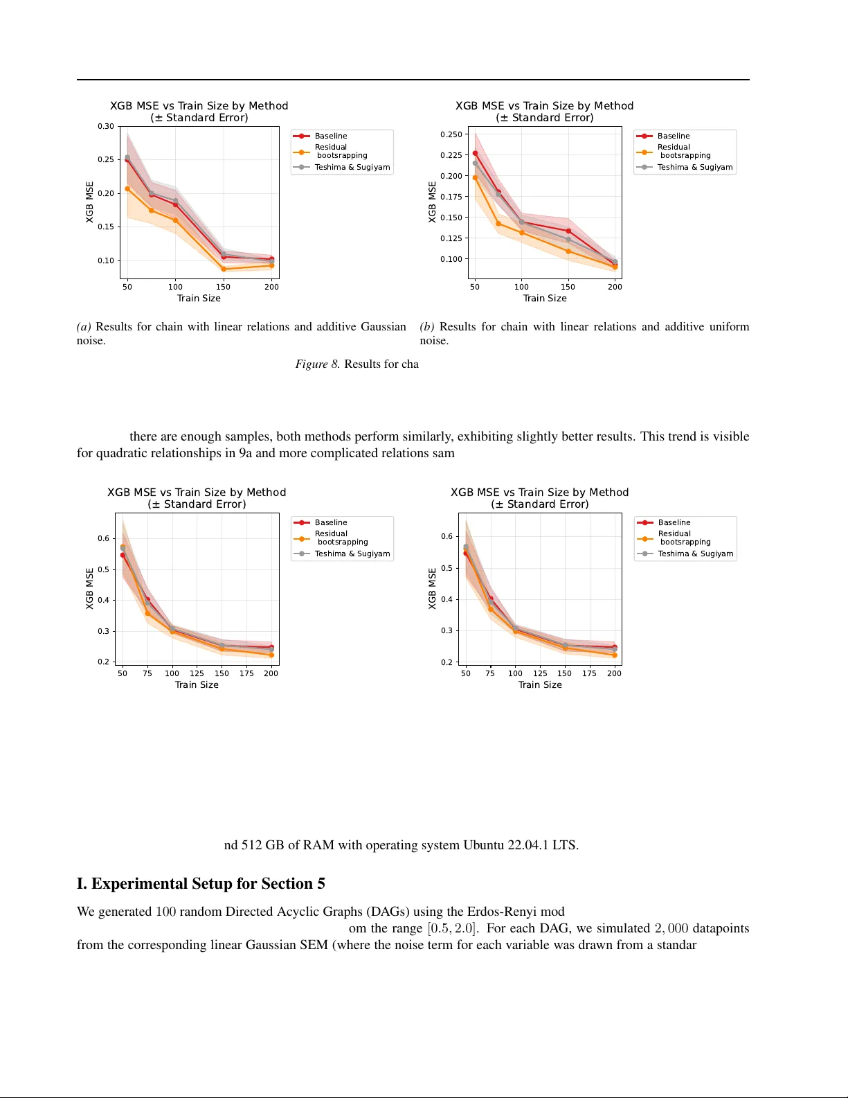
Data A ugmentation via Causal-Residual Bootstrapping Mateusz Gajewski 1 2 Sophia Xiao 3 Bijan Mazaheri 3 4 Abstract Data augmentation integrates domain kno wledge into a dataset by making domain-informed mod- iﬁcations to existing data points. For e xample, image data can be augmented by duplicating im- ages in different tints or orientations, thereby in- corporating the kno wledge that images may vary in these dimensions. Recent work by T eshima and Sugiyama has explored the inte gration of causal kno wledge (e.g, A causes B causes C) up to conditional independence equi valence. W e suggest a related approach for settings with ad- ditiv e noise that can incorporate information be- yond a Mark ov equi valence class. The approach, built on the principle of independent mecha- nisms, permutes the residuals of models built on marginal probability distributions. Predictive models built on our augmented data demonstrate improv ed accuracy , for which we provide theo- retical backing in linear Gaussian settings. 1. Introduction Large, comprehensive datasets have driv en a meteoric rise in the scale and capabilities of machine learning systems. Nev ertheless, data-sparse regimes remain, particularly in human health and science, where ﬁnancial and ethical bar- riers prohibit extensi ve data collection. By adding noise or anticipated transformations, data aug- mentation creates ne w training data points, thereby enhanc- ing the power of small datasets (W ang et al., 2024). Such augmentation strategies can be thought of as incorporating prior knowledge as new data. F or example, an augmented image dataset may account for known variations by v ary- ing lighting conditions and performing rotations (V an Dyk and Meng, 2001). 1 Pozna ´ n Univ ersity of T echnology , Pozna ´ n, Poland 2 AKCES NCBR, W arsaw , Poland 3 Thayer School of Engi- neering, Dartmouth, Hanover , NH, USA 4 Eric and W endy Schmidt Center, Broad Institute of MIT and Harvard, Cam- bridge, MA, USA. Correspondence to: Bijan Mazaheri < bi- jan.h.mazaheri@dartmouth.edu > . Pr eprint. Mar ch 17, 2026. Causal information is often represented in the form of a structural causal model (SCM), which is known to imply conditional independencies according to d-separation rules (Pearl, 2009). For example, consider a causal chain with A causes B and B causes C , and no other causal dependen- cies. Such a system is represented using a directed acyclic graph A → B → C , which is constrained by a Markov property of A ⊥ ⊥ C | B . Causal structures or conditional independencies are often known from prior experiments or by design. For example, randomized controlled trials (which are often small) are known to assign a randomized treatment ( T ) that contains no arro ws to or from other attributes of the participants ( X ). Such knowledge tells us that X ⊥ ⊥ T without the need for statistical testing. In other settings, causal structures can be learned using a process kno wn as causal discov ery (Squires and Uhler, 2023). Recently , foundation models based on the prior–data ﬁtted network (PFN) paradigm have gained traction in the ML community . This includes T abPFN (M ¨ uller et al.; Holl- mann et al., 2025), which was pre-trained on synthetic datasets generated using random structural causal models and Bayesian networks. Surprisingly , models pre-trained on synthetic data perform well on real-world datasets, seemingly beneﬁting from information that a causal struc- ture exists , ev en though the exact causal structure of the ev entual real-world data was not necessarily provided. This suggests that structural priors capture comple x indepen- dence relations in real-world data (Jiang et al., 2025). Seminal work by T eshima and Sugiyama (2021) has ex- plored incorporating causal information into data augmen- tation. In particular , they noted that conditional indepen- dencies allow entries of a dataset to be permuted. For ex- ample, if A ⊥ ⊥ B , then any observed v alue of A may be paired with any observed value of B . These permutations augment the data, e.g., a two-point set (0 , 0) , (1 , 1) may be augmented to (0 , 0) , (1 , 1) , (0 , 1) , (1 , 0) . Their approach shows moderate impro vement in prediction accurac y . The approach by T eshima and Sugiyama (2021) is limited in two ways. First, their approach requires reweighting data according to estimates of probability density , which thereby requires tuning the radius of a RBF kernel (Poinsot and Leite). Reweighting based on density was criticized 1 Data A ugmentation via Causal-Residual Bootstrapping by Mazaheri et al. (2020) for its dependence on tuning and general instability . Second, their approach is limited to augmenting conditional independence properties, which cannot account for causal direction. As such, the entire di- rected acyclic graph (D AG) cannot be utilized. Conditional independence information alone cannot fully specify a causal structure. For example, A → B → C , A ← B ← C , and A ← B → C display the same set of conditional independence properties, kno wn as a Markov equiv alence class (MEC), which is represented us- ing a “completed partial DA G” (CP-D A G) when there are no latent v ariables, and an acyclic directed mixed graph (ADMG) in the presence of latent confounding (Spirtes et al., 2000). Literature on causal disco very has sho wn that systems with nonlinear dependencies and Gaussian addi- tiv e noise contain additional information beyond the condi- tional independence properties that specify an MEC (Hoyer et al., 2008; Peters et al., 2014). In particular, nonlinear relationships shift Gaussian distributions to non-Gaussian distributions, yielding Gaussian residuals in the causal di- rection and non-Gaussian residuals in the anti-causal direc- tion. The goal of this paper is to address the limitation of T eshima and Sugiyama (2021) by incorporating informa- tion from the full causal structur e , including causal direc- tions. W e do this using the principle of independent mech- anisms, which states that if X causes Y , then the mecha- nism that turns X into Y (i.e., Pr( Y | X ) ) does not depend on how X is distributed ( Pr( X ) ) (Peters et al., 2017). As such, the distribution of residuals of the effect Y is inde- pendent from the value of the cause X . 1.1. Summary of Contributions W e begin by motiv ating the incorporation of causal struc- ture via data augmentation, rigorously demonstrating its ability to improve downstream regression tasks. Section 3 provides a theoretical justiﬁcation for this claim, sho w- ing that the improv ement in regression error scales propor- tionally to the inv erse of the starting dataset size (smaller datasets are improv ed more). Motiv ated by these theoretical results, we build on the work of T eshima and Sugiyama (2021) to dev elop a more broadly-applicable causal data augmentation approach, called “Causal-Residual Bootstrapping” (CRB). CRB is giv en in Section 4, utilizing the principle of independent mechanisms. The key observ ation is that predictions of variables from their direct causes should exhibit residuals that are independent from their predecessors’ values. As such, the residuals may be permuted, allo wing us to “boot- strap” the noise term and generate additional data. CRB satisﬁes two goals: it may preserve existing structural in- formation by augmenting data based on the output of a causal discovery algorithm, or it may help inject ne w struc- tural information into a dataset by lev eraging a known set of causal dependencies. T o emphasize the need for new methods like CRB, we demonstrate that genAI-based augmentation not only fails to capture causal structure but also contributes to its de- cline. Section 5 shows that V AEs, GANs, and diffusion models all weak en the performance of causal discovery algorithms run on their augmented datasets. Meanwhile, CRB and the approach by T eshima and Sugiyama (2021) preserve information about causal structure, as evidenced by unchanging performance in causal discovery . W e fur- ther test both of these causally-informed augmentation methods on linear models with non-Gaussian noise, which exhibit additional information beyond their MECs. In these experiments, the direct LinGAM algorithm (Shimizu et al., 2011) does not perform well on data augmented by T eshima and Sugiyama (2021)’ s approach, but retains per- formance for CRB. This demonstrates the added value of augmenting according to the full causal structure. Since many datasets do not satisfy the linear restrictions of our theoretical results, Section 6 provides an empirical study of CRB’ s improvements to downstream regression tasks. Experiments are done on both synthetic (Ap. G) and real datasets. These tests include both settings with kno wn causal structures and those with unkno wn causal structures learned from causal discov ery algorithms. 1.2. Related W orks Data A ugmentation. V arious domains have utilized prior knowledge for data augmentation. Modern tech- niques include generativ e adversarial networks (Bowles et al., 2018; T anaka and Aranha, 2019) and dif fusion mod- els (T rabucco et al., 2024). Myronenko (2018) utilized an auto-encoder with built-in randomness to regularize a model for brain-tumor segmentation to incorporate the prior belief that brain tumors are not location-speciﬁc. SMO TE (Chawla et al., 2002) uses data augmentation to address undersampling. Incorporating Causal Constraints. A series of works has explored incorporating successiv ely increasing amounts of causally-motiv ated constraints into re gres- sion. Early work by Chaudhuri et al. (2007) in vestigated improv ements in predictive regression tasks by zeroing entries of cov ariance matrices based on known marginal independencies. T eshima and Sugiyama (2021) expanded this notion to conditional independencies by incorporating information about the full MEC implied by a causal structure. This work also shifted from cov ariance matrix modiﬁcation to data augmentation, thereby relaxing the approach to non-Gaussian and non-linear settings. Still, 2 Data A ugmentation via Causal-Residual Bootstrapping this approach did not incorporate all causal information, omitting causal directions that are unspeciﬁed by an MEC. Most recently , augmenting datasets using the underlying (causal) Bayesian network has improved ﬁne-tuning of tabular foundation models in low-data regimes (B ¨ uhler et al., 2026). This approach was de veloped for a more specialized setting, but aligns with our motiv ation to use the entire causal structure for augmentation. Our approach eliminates the need for density estimation, used in B ¨ uhler et al. (2026) and T eshima and Sugiyama (2021). The approach can be thought of as a data-augmentation version of projecting distributions into a causal structure, a notion introduced by Mazaheri et al. (2025). Causal Structure and Pr edictive Models. Having ac- cess to the causal structure was shown to be beneﬁcial in many cases. This includes improving robustness to dis- tribution shifts (Lu et al., 2021; Heinze-Deml and Mein- shausen, 2021; Magliacane et al., 2018; Rojas-Carulla et al., 2018; Mazaheri et al., 2023), feature selection via Markov blankets (Tsamardinos and Aliferis, 2003; Y u et al., 2020), and measuring f airnes (Makhlouf et al., 2024; Maasch et al., 2025). All of these approaches are orthogo- nal to our own in that they model inv ariances that help build more robust machine learning models, but do not directly incorporate that information into the data. Such works mo- tiv ate our goal of incorporating this information directly into the dataset. Other Related W orks. Our work should not be confused with “causal boostrapping, ” proposed by Little and Badawy (2019), which in v olves re-sampling interv entional distrib u- tions from observational ones. 2. Preliminaries 2.1. Notation Con ventions W e will use the capital Roman alphabet (e.g., X, Y , A, B ) to denote endogenous (observ ed) random v ariables and the lowercase Roman alphabet to denote instantiations of those random variables (e.g., x i is a data measurement of X ). ε i will generally be used to represent random variables in the form of exogenous noise. W e will encounter two types of sets. Bold font will indi- cate sets of random variables, i.e. V = { V 1 , V 2 , . . . , V n } . Caligraphic font will generally be used to indicate sets of assignments (e.g., a dataset) to those random variables. For example, V ⟩ = { v (1) i , v (2) i , . . . v ( m ) i } . This paper will make use of directed acyclic graphs (D A Gs), e.g. G = ( V , E ) , for which we will need to reference parent sets. The vertices of these graphs will usually be inde xed as V = { V 1 , V 2 , . . . , V n } . W e de- note the parent set with respect to G with edges E using P A ( V j ) = { V i : ( V i , V j ) ∈ E } . 2.2. Structural Causal Models A structural causal model (SCM) is a set of random vari- ables V and a DA G G = ( V , E ) on those random vari- ables, representing causal dependencies (Pearl, 2009). For example, A → B indicates that A causes B . Graphical properties of G imply conditional independence properties on the random v ariables. D-separation rules, giv en in Pearl (2009), specify these graphical properties for conditional independence. Constraint-based causal discov- ery algorithms utilize these properties to ascertain graph- ical information using statistical tests for independence (Spirtes et al., 2000). Conditional independencies do not form a one-to-one map- ping with causal D A Gs; in fact, many causal D A Gs can cor- respond to the same set of conditional independence prop- erties. For this reason, many causal discovery algorithms only aim to reco ver these “Markov equivalence classes” (MECs). In general, all of the graphs in a MEC contain the same “undirected skeleton, ” formed by replacing all di- rected edges ( V i , V j ) with undirected edges { V i , V j } . In this sense, we can conclude that conditional independence contains full information about causal adjacency (the pres- ence or lack of a causal linkage), but incomplete informa- tion about the directions of those relationships. This incom- plete information is often represented in an ADMG called a completed partial D A G (CP-D A G) (Spirtes et al., 2000). For example, an undirected edge between A, B means that either A → B or B → A , but we do not kno w which one. 2.3. Structural Equation Models Parametric assumptions ha ve been utilized further to re- solve the output of causal disco very into a full causal D A G. In order to make these assumptions, we must augment SCMs with functional forms for the relationships between their random variables, V i = f i ( P A ( V i ) , ε i ) . (1) V i is therefore generated using a function of P A i , the direct causes of V i , and it’ s o wn source of e xogeneous noise ε i . It is common to assume that the exogenous noise sources are independent, i.e., ε i ⊥ ⊥ ε j for all i, j . A common assumption on Eq. (1) is additiv e noise, i.e., V i = f i ( P A ( V i )) + ε i . (2) In this framework, full identiﬁability of a causal model has been shown for linear f i ( · ) and non-Gaussian ε i (LiNGAM) (Shimizu, 2014) and non-linear f i ( · ) with Gaussian ε i s (Hoyer et al., 2008; Peters et al., 2014). 3 Data A ugmentation via Causal-Residual Bootstrapping 3. Causally Constrained Regression In this section, we summarize our theoretical results in Ap. B on the value of incorporating causal constraints into predictiv e regressions on observational data. For now , we only focus on the incorporation of the constraints within regression. Later (and in Ap. B.2), we show that our data augmentation method CRB, asymptotically approaches this constrained regression. The principle assumption of our theoretical results is that the data-generating process follows a linear Gaussian struc- tural causal model (SCM) as in Eq. (2), where f i are linear functions and ε i are Gaussian noise v ariables with variance V ar( ε i ) > 0 , and that the true causal D A G G = ( V , E ) is known. The full set of assumptions is stated formally in Ap. B. W e emphasize that violations of linearity and Gaus- sianity are heavily tested in our empirical sections. W e compare two approaches to ﬁtting a multi v ariate Gaus- sian distribution to the gi ven training data: 1. Unconstrained estimation: W e ﬁt a full multi variate Gaussian by computing the empirical covariance ma- trix ˆ Σ full without imposing any structural constraints. 2. DA G-constrained estimation: W e ﬁt a multiv ariate Gaussian distribution ˆ Σ D AG that respects the condi- tional independence structure implied by the graph G . Speciﬁcally , for any sets of variables A , B , and S , if A ⊥ ⊥ B | S holds in G according to d-separation, then the ﬁtted distribution must also satisfy A ⊥ ⊥ B | S . From the estimated covariance matrix, we can deriv e the re- gression coefﬁcients for predicting a tar get variable Y from features X : β = Σ − 1 XX Σ XY . (3) In the unconstrained case, this is equiv alent to standard or- dinary least squares (OLS) regression. Enforcing conditional independence constraints directly on the cov ariance matrix parameterization is non-tri vial, as these constraints translate into complex nonlinear relation- ships among the entries of Σ . Howe ver , such constraints are equiv alent to setting certain parameters to zero in the decomposition of the pr ecision matrix . Our results show that this sparsity pattern induces zeros in the Fisher infor- mation matrix, thereby decreasing the asymptotic v ariance of the estimated parameters. Speciﬁcally , we establish the following chain of results. First, the D A G-constrained estimator achiev es lower vari- ance in the Loewner ordering: Co v ( ˆ Σ D AG ) ⪯ Cov( ˆ Σ full ) . (4) This ordering transfers to the regression coef ﬁcients and, consequently , to the prediction error: E [MSE D AG pred ] ⩽ E [MSE full pred ] . (5) Moreov er , since the MLE parameters are asymptotically distributed as ˆ θ ∼ N ( θ , 1 N I − 1 ) , where I is the Fisher information matrix, we can quantify the expected impro ve- ment. The dif ference in prediction MSE scales as: E [MSE full pred ] − E [MSE D AG pred ] = C N , (6) where C > 0 is a constant that depends on the D A G struc- ture and the true distribution, but is independent of the sam- ple size N . Finally , we sho w that only DA G constraints inv olving the Markov boundary of the chosen label Y contribute to the improv ement in the prediction of Y . Although constraints among variables outside MB( Y ) decrease the variance of the estimated distribution parameters, this reduction does not translate to lower prediction MSE. 4. Causal-Residual Bootstrapping (CRB) In this section, we present a procedure that allows one to incorporate prior knowledge of a D AG by adding ne w aug- mented points to the dataset. W e do this by resampling residuals, leveraging the principle of independent mecha- nisms. The proposed method uses regression models in- stead of more complicated generativ e models and can be applied to non-linear and non-Gaussian settings, unlike the constrained regression discussed in our theoretical results. 4.1. Problem Setup and Input Speciﬁcation The augmentation procedure takes as input: • A directed acyclic graph (D A G) G = ( V , E ) repre- senting prior knowledge that we hav e about the data generation process and that we want to incorporate. • Dataset of values of n observed datapoints X . • A regression model class F such that f ∈ F : R d → R , d ∈ N (e.g., linear re gression, random forests, neu- ral networks) for the structural equations that can be ﬁtted to data. • M , the number of points to generate. The procedure outputs a new dataset ˜ X with augmented samples. 4.2. A ugmentation Procedure The augmentation procedure consists of two main phases: Learning Phase: W e learn the causal mechanisms by: 4 Data A ugmentation via Causal-Residual Bootstrapping 1. Computing a topological ordering π of the D A G G . 2. For each non-root variable X j , we: • Train a regression model ˆ f j ∈ F to predict X j from P A ( X j ) using the data V . • Compute residuals ˆ ε ( i ) j = x ( i ) j − ˆ f j ( P A ( x ( i ) j )) for all samples i = 1 , . . . , N . 3. For root variables, we store the vector of all observa- tions v j . Generation Phase: T o generate N synthetic samples, we: 1. For each synthetic sample m = 1 , . . . , M : • For each variable X j in topological order π : – If X j is a root node: sample ˜ x ( n ) j from the vector v j . – Otherwise: compute ˜ x ( m ) j = ˆ f j ( P A ( ˜ x ( m ) j )) + ˜ ε j , where ˜ ε j is randomly sampled from { ˆ ε ( i ) j } N i =1 . This procedure ensures that the generated data respects the structural equation frame work speciﬁed by the assumed SEM/SCM. As such, both the conditional independence properties (implied by the d-separation conditions of the MEC) and the la w of independent mechanisms (implied by causal direction) are enforced in the augmented data. The pseudocode is giv en in Alg. 1 in Ap. A. 4.3. CRB as Constrained Maximum Likelihood Under the assumptions of a linear SCM with Gaussian noise, when CRB uses linear regression to model each vari- able as a function of its parents, the method is asymptoti- cally equiv alent to performing global maximum likelihood estimation over the class of multi v ariate Gaussians con- strained by the D A G structure, as described in Section 3. Speciﬁcally , as the number of generated samples gro ws large, the CRB estimates con verge to the constrained MLE solution. The full deri vation is pro vided in Ap. B.2. Figure 1 validates these theoretical predictions empirically . W e tested two synthetic conﬁgurations: a simple chain ( A → B → C ) and a confounded structure ( A → B ← D , B → C ). In both cases, the observed MSE gap between unconstrained and D A G-constrained estimation follo ws the predicted C / N decay discussed in Section 3, with larger improv ements at smaller sample sizes. 5. Data A ugmentation and Causal Structure T o demonstrate the necessity of the proposed causal- residual-bootstrapping approach, we in vestigate whether F igur e 1. Empirical validation of MSE improvement rate. Left: Simple chain A → B → C . Right: Confounded structure A → B ← D , B → C . Both conﬁgurations show MSE im- prov ement following the predicted 1 / N decay . In both cases B is the predicted value deep learning augmentation techniques can preserve infor- mation about causal structures. W e ev aluated this using two causal disco very algorithms: The PC algorithm (Spirtes et al., 2000), which recov ers causal structures up to their MECs, and direct LinGAM (Shimizu et al., 2011), which recov ers the full causal structur e in settings with linear structural equations and non-Gaussian noise. Good perfor- mance, as measured by the Structural Hamming Distance (SHD), is taken to indicate that the augmented data pre- serves information about the causal structure. Poor per- formance indicates that the augmentation technique fails to preserve the ke y properties of data generated by that struc- ture. 5.1. Preser vation of MECs W e ﬁrst tested the preservation of information pertain- ing to the Markov equivalence class . W e ev aluated three generativ e methods: (1) Diffusion Models, (2) V aria- tional Autoencoders (V AEs), and (3) Generativ e Adversar - ial Networks (GANs). T ests were performed on 100 toy datasets generated from linear Gaussian SEMs correspond- ing to distinct and known D A Gs. For each method, new data points were generated using the trained augmentation model and appended to the original dataset. The PC algo- rithm was then applied to the augmented datasets to recover the causal graph. Further details for the experimental setup are giv en in Ap. I. Figure 2 illustrates the structural accuracy of the recovered graphs as a function of the number of augmented points. W e observe that as the number of synthetic datapoints in- creases, the SHD worsens across all baseline methods. This indicates that while these methods may achie ve high distri- butional ﬁdelity (lo w FID), they dilute the causal structural signal inherent in the original data. In contrast to causal- residual-bootstrapping, these causally-agnostic approaches fail to preserve the conditional independence relations re- quired for accurate causal discovery . Meanwhile, the per- formance of causal discovery is unaffected by augmenta- 5 Data A ugmentation via Causal-Residual Bootstrapping tion from CRB, as indicated by a non-increasing SHD. 5.2. Preser vation of Full Causal Structure While linear models with Gaussian additiv e noise cannot be recovered beyond their MECs, additional information is contained in non-Gaussian settings. Fig. 3 shows the performance of the direct LinGAM algorithm on data aug- mented with CRB and T eshima and Sugiyama (2021)’ s ADMGT ian approach. CRB continues to preserve all of the causal structure, while data added by ADMGTian weaken the algorithm’ s ability to orient causal direction despite re- taining conditional independencies. This demonstrates the added v alue of shifting from a purely MEC-based augmen- tation technique like ADMGT ian to CRB. 6. Empirical V alidation In this section, we empirically ev aluate the CRB method. Our experiments fall into two categories: (1) settings where the true causal graph is known and we seek to incorporate this structural information into the dataset, and (2) settings where we assess CRB as a principled approach to data aug- mentation, comparing it against existing methods where the graph is unkno wn, but learnable from causal discov ery . Ad- ditional synthetic data experiments are in Ap. G. 6.1. Experimental Setup Prediction Model. For all prediction tasks, we use XG- Boost (Chen and Guestrin, 2016), a gradient boosted tree model well-suited for tabular data. Hyperparame- ters are tuned using Optuna (Akiba et al., 2019) to en- sure good quality of prediction and ﬂexibility across di- verse datasets (Shwartz-Ziv and Armon, 2022; Grinsztajn et al., 2022). See Ap. F .1 for details. Ap. E includes addi- tional experiments with neural networks. A ugmentation Methods. W e compare CRB against se v- eral baseline augmentation methods: CTGAN (Bo wles et al., 2018), a GAN-based approach for tabular data; TV AE (Xu et al., 2019), a variational autoencoder adapted for tables; T abDDPM (K otelnikov et al., 2023), a diffusion- based generativ e model; ARF (W atson et al., 2023), which uses adversarial random forests for density estimation; NFLO W (Durkan et al., 2019), a normalizing ﬂow ap- proach. W e also compare against ADMGT ian (T eshima and Sugiyama, 2021), the prior method that incorporates causal structure into augmentation. Additionally , we in- clude a no-augmentation baseline where the predictor is trained solely on the original data. All baseline were grid seached for ev ery sample size and dataset; the details of which can be found in Ap. F .1 6.2. A ugmentation with Known Causal Graphs Our ﬁrst experiment inv estigates whether incorporating known causal structure into data augmentation can improv e downstream prediction accurac y . In this setting, the di- rect competitor to our method is ADMGT ian (T eshima and Sugiyama, 2021), which also lev erages causal graph infor- mation. W e additionally include non-causal augmentation methods (CTGAN, TV AE, DDPM, ARF , NFLO W) to ver- ify that any observed improvements stem from the prin- cipled use of causal structure rather than simply from in- creasing the number of training points. Evaluation Pr otocol. For ev aluation, we focus on the pre- diction accuracy of downstream regression tasks as mea- sured by mean squared error (MSE). Apart from practical use to improv e prediction, Jiang et al. (2025) utilized the av erage MSE across all possible label choices as a mea- sure of augmentation quality . Hence, we train many models on each dataset to predict each v ariable using the remain- ing v ariables as cov ariates. Predictors are trained on the augmented data, for which we e v aluate mean squared error (MSE) on held-out test data. Dataset: Causal Chambers. A fundamental challenge in ev aluating causal data augmentation methods is ob- taining real-world datasets where the true causal graph is known. This is a surprisingly dif ﬁcult requirement (Brouil- lard et al., 2024), as most datasets lack absolute kno wl- edge of a ground-truth graph and rely on expert opinions that may contain errors. T o address this challenge, we uti- lize data from the Causal Chamber (Gamella et al., 2025), a physical experimental platform speciﬁcally designed for causal research. The Causal Chamber consists of mod- ular hardware components—including light sources, sen- sors, polarizers, and other optical elements—whose phys- ical interactions deﬁne a known causal structure. Because the data-generating process is governed by well-understood physical la ws, the causal graph is determined by the exper - imental apparatus itself rather than by statistical estimation or expert judgment. This provides a unique opportunity to ev aluate causal methods against ground truth, but it is worth noting that similar settings emerge in many engineer- ing applications. Results. Figure 4 presents the mean MSE across all vari- ables for each augmentation method using 100 training samples. CRB achiev es the lo west mean MSE, outperform- ing both the no-augmentation baseline and all competing methods. Notably , ADMG-T ian and the other non-causal methods (ARF , CTGAN, TV AE) perform worse than no augmentation, suggesting that naiv e augmentation without causal constraints can degrade predicti ve performance. The improvement from CRB is not uniform across vari- ables. Figure 5 illustrates two contrasting cases: the blue 6 Data A ugmentation via Causal-Residual Bootstrapping (a) Diffusion Model (b) V ariational Autoencoder (c) GAN (d) CRB F igur e 2. Performance of the PC algorithm on datasets augmented by alternativ e methods. The plots show the average Structural Hamming Distance (SHD) between the true D AG and the estimated CPD AG returned by the PC algorithm as the number of augmented points increases; the shaded region indicates one standard de viation. Higher SHD indicates worse performance. (a) ADMGT ian (b) CRB F igur e 3. Performance of DirectLINGAM algorithm. None CRB ADMG T ian ARF CTGAN DDPM TV AE Augmenter 0.0 0.1 0.2 0.3 0.4 0.5 0.6 0.7 Mean MSE Mean MSE by Augmenter (Known Graph) with 95% Bootstrap CI F igur e 4. Mean MSE across all variables by augmentation method (Known Graph, n = 100 ). Lower is better . CRB achie ves the best performance, while non-causal augmenters often increase error relativ e to no augmentation. variable, where CRB substantially reduces MSE compared to all other methods, and the ir 1 v ariable, where im- prov ements are more modest. T able 1 summarizes the best and worst per-v ariable performance for each augmenter rel- ativ e to no augmentation. CRB shows the largest improv e- ment on its best variable ( green , MSE reduced by 0.23) while exhibiting minimal degradation on its worst variable ( ir 3 , MSE increased by only 0.006). In contrast, other methods show substantial degradation on some v ariables— for example, ARF increases MSE by 0.89 on angle 1 . Full per-v ariable results are provided in Ap. C. None CRB ADMG T ian ARF CTGAN DDPM TV AE Augmenter 0.0 0.1 0.2 0.3 0.4 0.5 0.6 0.7 MSE MSE by Augmenter (Known Graph) with 95% Bootstrap CI V ariable blue ir_1 F igur e 5. Per-v ariable MSE comparison (Known Graph, n = 100 ). T able 1. Best and worst per-v ariable performance relative to no augmentation. “Improv . ” corresponds to MSE reduction (positi ve = better) on the best performing variable; “W orsen. ” corresponds to MSE increase on the worst-performing v ariable. Method Best V ar . Improv . W orst V ar. W orsen. CRB green 0.227 ir 3 0.006 ADMG-T ian angle 1 0.000 l 21 0.169 ARF l 12 0.118 angle 1 0.889 CTGAN l 12 0.001 green 0.451 DDPM red 0.016 l 11 0.244 TV AE current − 0.024 green 0.221 6.3. Scaling Our theoretical results for linear models suggest that the improv ement from incorporating causal structure dimin- ishes as the number of training samples grows. T o empir- 7 Data A ugmentation via Causal-Residual Bootstrapping ically v alidate this prediction, we conducted experiments on the Causal Chamber dataset with varying sample sizes. As shown in Fig. 7, this intuition from simple models aligns with observations from the real-world dataset. CRB outper- forms no augmentation for small data sizes, and the differ - ence gradually decreases for larger datasets. On the other hand, the ADMGT ian method fails to outperform no aug- mentation for all sample sizes. 50 100 200 400 T rain Size (samples) 0.375 0.400 0.425 0.450 0.475 0.500 0.525 0.550 Mean MSE Mean MSE vs Sample Size (Known Graph) with 95% Bootstrap CI Augmenter ADMG T ian CRB None F igur e 6. Mean MSE across all v ariables as sample size increases (Known Graph). Lower is better . CRB maintains strong perfor- mance across sample sizes. 6.4. Unknown graph In this section, we ev aluate the setting where the true causal graph is unknown and must be learned from data. Our goal is to demonstrate that CRB can serve as an effecti ve syn- thetic data generation method, comparable to the best data augmentation approaches, even when relying on disco v- ered rather than kno wn causal structure. For these tests, we ev aluate our metrics on ne w data points generated by the augmentation method, excluding the original dataset. The “no augmentation” case includes only the original data. For both CRB and ADMG-T ian, we employ a causal dis- cov ery step prior to augmentation. Follo wing T eshima and Sugiyama (2021), we use the DirectLiNGAM (Shimizu et al., 2011) algorithm to learn the causal graph from the observed data (details in Ap. F .2). W e continue to use the Causal Chamber dataset, as we kno w the underlying sys- tem satisﬁes the assumptions required by CRB: there e xists a true causal graph, and the data contain no unobserved confounders or self-loops. Additionally , to facilitate com- parison with prior work, we e v aluate on se veral widely rec- ognized datasets used by T eshima and Sugiyama (2021): Sachs (Sachs et al., 2005), Boston Housing (Harrison Jr and Rubinfeld, 1978), Red W ine Quality , and White W ine Quality (Cortez et al., 2009). T able 2 presents the mean MSE across all v ariables for 100 samples. The results for bigger samples sizes and distri- bution metrics are in Ap. D. Overall, CRB and T abDDPM are the two best-performing methods, aligning with previ- ous observations (Jiang et al., 2025). On Causal Chambers, CRB achie ves the best performance (0.383), outperforming all methods, including T abDDPM (0.483) and no augmen- tation (0.422). The same holds for White W ine, where CRB outperforms all augmentation methods and performs com- parably to no augmentation. For Red W ine, T abDDPM is the best augmenter , performing on par with no augmenta- tion, with CRB as the second best. On Sachs, all augmen- tation methods help, with T abDDPM, CRB, and ADMG- T ian performing best. On Boston, T abDDPM performs best with CRB again in second place. 7. Conclusion W e provide a simple approach to augmenting data using a known causal structure. This approach helps integrate known causal knowledge into a dataset, either from previ- ous e xperiments or a learned causal structure (thereby inte- grating the assumption of an existing causal structure). Our extensi ve empirical results show promising improve- ment in prediction tasks. Compared to the current state of the art, our approach is a more-consistent method for in- corporating causal knowledge into data augmentation that does not require density estimation. The downside of our approach is its reliance on trained models, whose perfor- mance declines with weaker signals. The results from experiments with learned causal graphs highlight important considerations when combining causal discov ery with data augmentation. Errors or inaccuracies in the learned graph structure can signiﬁcantly limit the bene- ﬁts of structure-based augmentation, as incorrect edge ori- entations or missing edges may violate the independence assumptions on which our method relies. As methods for causal discovery improve, we expect causal data augmen- tation to become signiﬁcantly more useful. Furthermore, different causal discovery methods operate under varying assumptions. These underlying assumptions can interact with the augmentation procedure in complex and some- times unpredictable ways, because the learned graph may be valid only under the speciﬁc conditions assumed by the discov ery algorithm. It is not immediately obvious which causal discovery algorithms are optimal for data augmen- tation. Understanding these interactions and identifying which properties of learned causal graphs are most critical for ef fective augmentation are interesting and important ar- eas for future work. Data augmentation that preserves and reinforces causal structure has potentially vast applications for personal pri- vac y because of its ability to generate synthetic points with no direct personal connections while retaining both inter- variable relationships and causal structure. 8 Data A ugmentation via Causal-Residual Bootstrapping T able 2. Mean MSE ( ↓ ) across datasets with learned causal graph (100 samples). 95% CI in parentheses. Full results in Ap. D. Method Boston Sachs W ine (red) W ine (white) Causal Chamber ADMGT ian 1.886 (1.45, 2.13) 0.596 (0.54, 0.67) 0.831 (0.79, 0.86) 0.874 (0.83, 0.93) 0.474 (0.47, 0.48) ARF 0.625 (0.59, 0.70) 0.830 (0.81, 0.85) 0.981 (0.92, 1.02) 1.034 (1.03, 1.04) 0.738 (0.71, 0.76) CTGAN 0.612 (0.58, 0.66) 0.876 (0.81, 0.95) 0.769 (0.73, 0.80) 0.912 (0.86, 1.02) 0.579 (0.55, 0.61) CRB 0.457 (0.45, 0.47) 0.766 (0.55, 1.50) 0.635 (0.62, 0.65) 0.689 (0.67, 0.71) 0.383 (0.38, 0.38) DDPM 0.371 (0.36, 0.39) 0.545 (0.48, 0.71) 0.586 (0.58, 0.60) 0.757 (0.73, 0.78) 0.483 (0.48, 0.49) NFLO W 0.489 (0.48, 0.51) 0.783 (0.72, 0.85) 0.668 (0.63, 0.72) 0.799 (0.77, 0.84) 0.537 (0.50, 0.60) None 0.364 (0.35, 0.38) 0.998 (0.99, 1.00) 0.587 (0.58, 0.60) 0.679 (0.67, 0.68) 0.422 (0.42, 0.43) TV AE 0.531 (0.50, 0.57) 0.795 (0.72, 0.86) 0.764 (0.73, 0.80) 0.837 (0.80, 0.90) 0.543 (0.53, 0.55) Acknowledgements Support for Bijan Mazaheri and Sophia Xiao was pro- vided by the Advanced Research Concepts (ARC) COM- P ASS program, sponsored by the Defense Advanced Re- search Projects Agency (DARP A) under agreement number HR001-25-3-0212. Impact Statement This paper presents work whose goal is to advance the ﬁeld of machine learning. There are many potential societal con- sequences of our work, none of which we feel must be speciﬁcally highlighted here. Use of the Boston Housing Dataset (Harrison Jr and Rubinfeld, 1978) has been crit- icized. Howe ver , since the dataset is used T eshima and Sugiyama (2021), we elected to also include it for the sake of comparison. R E F E R E N C E S T akuya Akiba, Shotaro Sano, T oshihiko Y anase, T akeru Ohta, and Masanori K oyama. Optuna: A next- generation hyperparameter optimization framew ork. In Pr oceedings of the 25th A CM SIGKDD international confer ence on knowledge discovery & data mining , pages 2623–2631, 2019. Ahmed Alaa, Boris V an Breugel, Evgeny S Sav eliev , and Mihaela V an Der Schaar . Ho w faithful is your synthetic data? sample-level metrics for ev aluating and auditing generativ e models. In International conference on ma- chine learning , pages 290–306. PMLR, 2022. Christopher Bo wles, Liang Chen, Ricardo Guerrero, Paul Bentley , Roger Gunn, Ale xander Hammers, David Alexander Dickie, Maria V ald ´ es Hern ´ andez, Joanna W ardlaw , and Daniel Rueckert. Gan augmenta- tion: Augmenting training data using generative adver- sarial networks. arXiv pr eprint arXiv:1810.10863 , 2018. Philippe Brouillard, Chandler Squires, Jonas W ahl, K on- rad P K ording, Karen Sachs, Alexandre Drouin, and Dhanya Sridhar . The landscape of causal discov ery data: Grounding causal discov ery in real-world applications. arXiv pr eprint arXiv:2412.01953 , 2024. Magnus B ¨ uhler , Lennart Purucker , and Frank Hut- ter . Causal data augmentation for robust ﬁne- tuning of tabular foundation models. arXiv preprint arXiv:2601.04110 , 2026. Sanjay Chaudhuri, Mathias Drton, and Thomas S Richard- son. Estimation of a covariance matrix with zeros. Biometrika , 94(1):199–216, 2007. Nitesh V Chawla, K e vin W Bo wyer, Lawrence O Hall, and W Philip Kegelme yer . Smote: synthetic minority over - sampling technique. Journal of artiﬁcial intellig ence r e- sear ch , 16:321–357, 2002. T ianqi Chen and Carlos Guestrin. Xgboost: A scalable tree boosting system. In Pr oceedings of the 22nd acm sigkdd international confer ence on knowledge discovery and data mining , pages 785–794, 2016. Paulo Cortez, A. Cerdeira, F . Almeida, T . Matos, and J. Reis. W ine Quality . UCI Machine Learning Repos- itory , 2009. DOI: https://doi.org/10.24432/ C56S3T . Conor Durkan, Artur Bekasov , Iain Murray , and George Papamakarios. Neural spline ﬂows. Advances in neural information pr ocessing systems , 32, 2019. Juan L Gamella, Jonas Peters, and Peter B ¨ uhlmann. Causal chambers as a real-w orld physical testbed for ai method- ology . Nature Machine Intelligence , 7(1):107–118, 2025. L ´ eo Grinsztajn, Edouard Oyallon, and Ga ¨ el V aroquaux. Why do tree-based models still outperform deep learning on typical tabular data? Advances in neural information pr ocessing systems , 35:507–520, 2022. David Harrison Jr and Daniel L Rubinfeld. Hedonic hous- ing prices and the demand for clean air . J ournal of en- vir onmental economics and management , 5(1):81–102, 1978. 9 Data A ugmentation via Causal-Residual Bootstrapping Christina Heinze-Deml and Nicolai Meinshausen. Con- ditional variance penalties and domain shift robustness. Machine Learning , 110(2):303–348, 2021. Noah Hollmann, Samuel M ¨ uller , Lennart Purucker , Arjun Krishnakumar , Max K ¨ orfer , Shi Bin Hoo, Robin T ibor Schirrmeister , and Frank Hutter . Accurate predictions on small data with a tabular foundation model. Natur e , 637(8045):319–326, 2025. Patrik O. Hoyer , Dominik Janzing, Joris M. Mooij, Jonas Peters, and Bernhard Sch ¨ olkopf. Nonlinear causal discov ery with additive noise models. In D. Koller , D. Schuurmans, Y . Bengio, and L. Bottou, editors, Ad- vances in Neur al Information Pr ocessing Systems 21 , pages 689–696, V ancouver , BC, Canada, June 2008. Curran Associates. NIPS 2008. Xiangjian Jiang, Nikola Simidjievski, and Mateja Jamnik. T abstruct: Measuring structural ﬁdelity of tabular data. arXiv pr eprint arXiv:2509.11950 , 2025. Akim K otelnikov , Dmitry Baranchuk, Ivan Rubachev , and Artem Babenko. T abddpm: Modelling tabular data with diffusion models. In International confer ence on ma- chine learning , pages 17564–17579. PMLR, 2023. Max A Little and Reham Badawy . Causal bootstrapping. arXiv pr eprint arXiv:1910.09648 , 2019. Chaochao Lu, Y uhuai W u, Jos ´ e Miguel Hern ´ andez-Lobato, and Bernhard Sch ¨ olkopf. In variant causal representation learning for out-of-distribution generalization. In Inter- national Conference on Learning Representations , 2021. Jacqueline Maasch, Kyra Gan, V iolet Chen, Agni Or- fanoudaki, Nil-Jana Akpinar , and Fei W ang. Local causal disco very for structural evidence of direct dis- crimination. In Proceedings of the AAAI Confer ence on Artiﬁcial Intelligence , volume 39, pages 19349–19357, 2025. Sara Magliacane, Thijs V an Ommen, T om Claassen, Stephan Bongers, Philip V ersteeg, and Joris M Mooij. Domain adaptation by using causal inference to predict in variant conditional distributions. Advances in neural information pr ocessing systems , 31, 2018. Karima Makhlouf, Sami Zhioua, and Catuscia Palamidessi. When causality meets fairness: A survey . J ournal of Logical and Algebraic Methods in Pr ogr amming , 141: 101000, 2024. Bijan Mazaheri, Siddharth Jain, and Jehoshua Bruck. Robust correction of sampling bias using cumulati ve distribution functions. In H. Larochelle, M. Ran- zato, R. Hadsell, M.F . Balcan, and H. Lin, editors, Advances in Neural Information Pr ocessing Systems , volume 33, pages 3546–3556. Curran Associates, Inc., 2020. URL https://proceedings. neurips.cc/paper/2020/file/ 24368c745de15b3d2d6279667debcba3- Paper. pdf . Bijan Mazaheri, Atalanti Mastakouri, Dominik Janzing, and Michaela Hardt. Causal information splitting: en- gineering proxy features for robustness to distrib ution shifts. In Uncertainty in Artiﬁcial Intelligence , pages 1401–1411. PMLR, 2023. Bijan Mazaheri, Jiaqi Zhang, and Caroline Uhler . Meta- dependence in conditional independence testing. arXiv pr eprint arXiv:2504.12594 , 2025. Samuel M ¨ uller , Noah Hollmann, Sebastian Pineda Arango, Josif Grabocka, and Frank Hutter . T ransformers can do bayesian inference. In International Confer ence on Learning Repr esentations . Andriy Myronenko. 3d mri brain tumor segmentation using autoencoder re gularization. In International MICCAI brainlesion workshop , pages 311–320. Springer , 2018. Judea Pearl. Causality . Cambridge univ ersity press, 2009. Jonas Peters, Joris M. Mooij, Dominik Janzing, and Bern- hard Sch ¨ olkopf. Causal discov ery with continuous ad- ditiv e noise models. J ournal of Machine Learning Re- sear ch , 15(58):2009–2053, 2014. Jonas Peters, Dominik Janzing, and Bernhard Sch ¨ olkopf. Elements of causal infer ence: foundations and learning algorithms . The MIT press, 2017. Audrey Poinsot and Alessandro Leite. A guide for practical use of admg causal data augmentation. In ICLR 2023 W orkshop on Pitfalls of limited data and computation for T rustworthy ML . Zhaozhi Qian, Rob Davis, and Mihaela V an Der Schaar . Synthcity: a benchmark frame work for div erse use cases of tabular synthetic data. Advances in neural information pr ocessing systems , 36:3173–3188, 2023. Mateo Rojas-Carulla, Bernhard Sch ¨ olkopf, Richard T urner , and Jonas Peters. In variant models for causal transfer learning. J ournal of Machine Learning Resear ch , 19 (36):1–34, 2018. Karen Sachs, Omar Perez, Dana Pe’er , Douglas A Lauf- fenbur ger , and Garry P Nolan. Causal protein-signaling networks deri ved from multiparameter single-cell data. Science , 308(5721):523–529, 2005. Shohei Shimizu. Lingam: Non-gaussian methods for esti- mating causal structures. Behaviormetrika , 41(1):65–98, 2014. 10 Data A ugmentation via Causal-Residual Bootstrapping Shohei Shimizu, T akanori Inazumi, Y asuhiro Sogawa, Aapo Hyvarinen, Y oshinobu Kaw ahara, T akashi W ashio, Patrik O Hoyer , Kenneth Bollen, and Patrik Hoyer . Di- rectlingam: A direct method for learning a linear non- gaussian structural equation model. Journal of Machine Learning Resear ch-JMLR , 12(Apr):1225–1248, 2011. Ravid Shwartz-Zi v and Amitai Armon. T abular data: Deep learning is not all you need. Information Fusion , 81: 84–90, 2022. Peter Spirtes, Clark N Glymour , and Richard Scheines. Causation, pr ediction, and sear ch . MIT press, 2000. Chandler Squires and Caroline Uhler . Causal structure learning: A combinatorial perspective. F oundations of Computational Mathematics , 23(5):1781–1815, 2023. Fabio Henrique Kiyoiti Dos Santos T anaka and Claus Aranha. Data augmentation using gans. arXiv pr eprint arXiv:1904.09135 , 2019. T akeshi T eshima and Masashi Sugiyama. Incorporating causal graphical prior knowledge into predictiv e mod- eling via simple data augmentation. In Uncertainty in Artiﬁcial Intelligence , pages 86–96. PMLR, 2021. Brandon T rabucco, Kyle Doherty , Max A Gurinas, and Ruslan Salakhutdino v . Effecti ve data augmentation with diffusion models. In The T welfth International Confer- ence on Learning Repr esentations , 2024. URL https: //openreview.net/forum?id=ZWzUA9zeAg . Ioannis Tsamardinos and Constantin F Aliferis. T owards principled feature selection: Relev ancy , ﬁlters and wrap- pers. In International W orkshop on Artiﬁcial Intelligence and Statistics , pages 300–307. PMLR, 2003. David A V an Dyk and Xiao-Li Meng. The art of data augmentation. Journal of Computational and Graphical Statistics , 10(1):1–50, 2001. Zaitian W ang, Pengfei W ang, Kunpeng Liu, Pengyang W ang, Y anjie Fu, Chang-Tien Lu, Charu C Aggarwal, Jian Pei, and Y uanchun Zhou. A comprehensiv e survey on data augmentation. arXiv pr eprint arXiv:2405.09591 , 2024. David S W atson, Kristin Blesch, Jan Kapar, and Marvin N Wright. Adversarial random forests for density estima- tion and generati ve modeling. In International Con- fer ence on Artiﬁcial Intelligence and Statistics , pages 5357–5375. PMLR, 2023. Lei Xu, Maria Skoularidou, Alfredo Cuesta-Infante, and Kalyan V eeramachaneni. Modeling tabular data using conditional gan. Advances in neural information pr o- cessing systems , 32, 2019. Kui Y u, Xianjie Guo, Lin Liu, Jiuyong Li, Hao W ang, Zhaolong Ling, and Xindong W u. Causality-based fea- ture selection: Methods and ev aluations. ACM Comput- ing Surve ys (CSUR) , 53(5):1–36, 2020. Zilong Zhao, Aditya Kunar , Robert Birk e, and L ydia Y Chen. Ctab-gan: Effecti ve table data synthesizing. In Asian confer ence on machine learning , pages 97–112. PMLR, 2021. 11 Supplementary Materials A. Algorithm Pseudocode Alg. 1 provides the pseudocode for the CRB algorithm. Algorithm 1 Causal Data Augmentation Require: D A G G , dataset V , regression model class F , number of synthetic samples M Ensure: Synthetic dataset ˜ X = { ˜ x (1) , . . . , ˜ x ( M ) } 1: // Learning Phase 2: π ← T opologicalSort ( G ) { Get causal ordering } 3: for each v ariable X j ∈ V in order π do 4: P A j ← Parents ( X j , G ) 5: if | P A j | = 0 then 6: Dist j ← { x (1) j , . . . , x ( N ) j } { Store empirical distrib ution } 7: else 8: X P A j ← [ P A j values from D ] { P arent features } 9: y j ← [ x (1) j , . . . , x ( N ) j ] { T arget v alues } 10: ˆ f j ← Train ( F , X P A j , y j ) { Learn regression model } 11: ˆ y j ← ˆ f j ( X P A j ) { Predictions } 12: ˆ ε j ← y j − ˆ y j { Compute residuals } 13: end if 14: end for 15: 16: // Generation Phase 17: ˜ D ← ∅ 18: for m = 1 to M do 19: ˜ x ( m ) ← empty vector 20: for each v ariable X j ∈ V in order π do 21: if | P A j | = 0 then 22: ˜ x ( m ) j ← Sample ( Dist j ) { Sample from marginal } 23: else 24: ˜ x ( m ) P A j ← [ parent values from ˜ x ( m ) ] 25: ˜ ε j ← Sample ( ˆ ε j ) { Sample residual } 26: ˜ x ( m ) j ← ˆ f j ( ˜ x ( m ) P A j ) + ˜ ε j { Generate value } 27: end if 28: end for 29: ˜ D ← ˜ D ∪ { ˜ x ( m ) } 30: end for 31: return ˜ D B. Theoretical Analysis of Causal Structur e in Regression B.1. Introduction and Setup In this section, we in vestigate how incorporating additional information in the form of graph knowledge can improve the quality of prediction for regression tasks. W e present a theoretical analysis of this setting, establishing conditions under which knowledge of the causal D A G prov ably reduces estimation variance and, consequently , prediction error . Throughout this section, we operate under the following assumptions: Assumption B.1 (Linear Gaussian Structural Causal Model) . The data-generating process follows a linear Gaussian struc- tural causal model (SCM). That is, for each vari able V j ∈ V , for j = 1 , 2 , . . . , n , the corresponding structural equation Data A ugmentation via Causal-Residual Bootstrapping has the form V j = X V i ∈ P A ( V j ) β ij V i + ε j , (7) where β ij ∈ R are the structural coefﬁcients and ε j ∼ N (0 , σ 2 j ) are mutually independent Gaussian noise terms. This system can be written in matrix form as V = BV + ε , (8) where B ∈ R d × d is a strictly lower-triangular matrix (under a topological ordering of the variables) of structural coefﬁ- cients such that B j i = β ij if V i ∈ P A ( V j ) and 0 otherwise, and ε ∼ N ( 0 , Σ ε ) is a multi variate Gaussian noise vector with cov ariance matrix Σ ε = diag ( σ 2 1 , . . . , σ 2 d ) . Assumption B.2 (Non-Degenerate Noise) . All noise variances are strictly positive, i.e., σ 2 j > 0 for all j ∈ { 1 , . . . , n } . This ensures that each variable e xhibits genuine stochastic variation be yond what is explained by its parents. Assumption B.3 (Known Causal Structure) . W e have access to the true causal D A G G = ( V , E ) that generated the data. The graph correctly speciﬁes all direct causal relationships: ( V i , V j ) ∈ E if and only if V i is a direct cause of V j in the underlying SCM. Under these assumptions, we establish three main results: (1) Causal-Residual Bootstrapping is asymptotically equivale nt to constrained maximum likelihood estimation, (2) enforcing correct DA G constraints prov ably reduces parameter variance, and (3) this variance reduction translates to impro ved prediction accurac y as measured by mean squared error . B.2. Equivalence to Constrained Maximum Lik elihood Estimation W e now sho w that Causal-Residual Bootstrapping with linear regression is equiv alent to maximum likelihood estimation under the D A G-constrained model. B . 2 . 1 . L I K E L I H O O D F AC T O R I Z A T I O N O V E R T H E DA G Under the linear Gaussian SCM (Assumption B.1), each conditional distribution tak es the form: V j | P A ( V j ) ∼ N   X V i ∈ P A ( V j ) β ij V i , σ 2 j   . (9) By the Markov property induced by the D A G G , the joint distribution factorizes according to the graph structure: p ( V 1 , V 2 , . . . , V n ) = n Y j =1 p ( V j | P A ( V j )) . (10) T aking logarithms, the log-likelihood decomposes as a sum over local conditional log-lik elihoods: log p ( V 1 , V 2 , . . . , V n ) = n X j =1 log p ( V j | P A ( V j )) . (11) Giv en a dataset D = { ( v ( i ) 1 , . . . , v ( i ) n ) } N i =1 of N i.i.d. observations, the total log-likelihood is: ℓ ( θ ; D ) = N X i =1 n X j =1 log p ( v ( i ) j | v ( i ) P A ( j ) ; θ j ) , (12) where θ j = ( β j , σ 2 j ) denotes the parameters of the j -th conditional distribution, with β j = ( β ij ) V i ∈ P A ( V j ) . 13 Data A ugmentation via Causal-Residual Bootstrapping B . 2 . 2 . D E C O M P O S I T I O N I N T O I N D E P E N D E N T L O C A L P R O B L E M S A key observ ation is that the parameters θ j for different v ariables j appear in disjoint terms of the log-likelihood. Speciﬁ- cally , rearranging the sums: ℓ ( θ ; D ) = n X j =1 N X i =1 log p ( v ( i ) j | v ( i ) P A ( j ) ; θ j ) | {z } ℓ j ( θ j ) . (13) Since θ j only appears in ℓ j ( θ j ) , the global maximization problem separates into n independent local problems: argmax θ ℓ ( θ ; D ) = n argmax θ j ℓ j ( θ j ) o n j =1 . (14) B . 2 . 3 . L O C A L M L E E Q U A L S L E A S T S Q UA R E S R E G R E S S I O N For the Gaussian conditional V j | P A ( V j ) ∼ N ( v ⊤ P A ( j ) β j , σ 2 j ) , the local log-likelihood is: ℓ j ( β j , σ 2 j ) = − N 2 log(2 π σ 2 j ) − 1 2 σ 2 j N X i =1  v ( i ) j − v ( i ) ⊤ P A ( j ) β j  2 . (15) Maximizing with respect to β j is equiv alent to minimizing the sum of squared residuals: ˆ β j = argmin β j N X i =1  v ( i ) j − v ( i ) ⊤ P A ( j ) β j  2 , (16) which is precisely ordinary least squares (OLS) regression of V j on its parents P A ( V j ) . The MLE for the noise variance is the empirical v ariance of the residuals: ˆ σ 2 j = 1 N N X i =1  v ( i ) j − v ( i ) ⊤ P A ( j ) ˆ β j  2 . (17) Proposition B.4 (CRB Learning Phase Equals Constrained MLE) . The learning phase of Causal-Residual Bootstr apping, which performs linear re gression of each variable V j on its parents P A ( V j ) , computes the maximum likelihood estimates under the D A G-constrained linear Gaussian model. Pr oof. The CRB learning phase ﬁts ˆ f j by regressing V j on P A ( V j ) . W ith linear regression, this solv es: ˆ β j = argmin β j N X i =1  v ( i ) j − v ( i ) ⊤ P A ( j ) β j  2 . As shown above, this is exactly the local MLE for θ j . Since the global MLE decomposes into independent local MLEs, and CRB solves each local problem, it achie ves the global MLE. Remark B.5 . The DA G structure constrains which parameters are estimated: only coef ﬁcients β ij for edges ( V i , V j ) ∈ E are included. Coefﬁcients for non-edges are implicitly constrained to zero. This is in contrast to an unconstrained model that would estimate a full cov ariance matrix without imposing the DA G structure. B.3. Correspondence Between Pr ecision Factorization and D A G Constraints Here we show that D A G constraints on a linear Gaussian SCM correspond to constraints on the U factor of the UDU decomposition of the precision matrix of V . 14 Data A ugmentation via Causal-Residual Bootstrapping B . 3 . 1 . C OV A R I A N C E M ATR I X R E P R E S E N TA T I O N The linear Gaussian SCM from Assumption B.1 corresponds to a multiv ariate Gaussian distribution ov er n variables V = ( V 1 , . . . , V n ) . It is fully characterized by its mean vector µ ∈ R n and cov ariance matrix Σ ∈ R n × n . W ithout loss of generality , we assume zero mean ( µ = 0 ), as centering does not affect the causal structure. By deﬁnition, the cov ariance matrix Σ is symmetric positi ve semi-deﬁnite. Under Assumption B.2 (non-degenerate noise), the cov ariance matrix of V is strictly positive deﬁnite ( Σ ≻ 0 ); therefore, its in verse, known as the precision matrix and denoted as Σ − 1 := Ω exists and is also symmetric positi ve deﬁnite. B . 3 . 2 . L D L A N D U D U D E C O M P O S I T I O N Any symmetric positi ve deﬁnite matrix A ∈ R n admits a unique LDL decomposition A = LDL ⊤ , (18) where: • L ∈ R n × n is a lower triangular matrix with ones on the diagonal ( L ii = 1 for all i ), • D = diag( d 1 , . . . , d n ) ∈ R n × n is a diagonal matrix with strictly positiv e entries ( d i > 0 ). The LDL decomposition is closely related to the standard Cholesky decomposition A = CC ⊤ , where C = LD 1 / 2 . Similarly , any symmetric positi ve deﬁnite matrix A ∈ R n admits a unique UDU decomposition A = UDU ⊤ , (19) where: • U ∈ R n × n is an upper triangular matrix with ones on the diagonal ( U ii = 1 for all i ), • D = diag( d ′ 1 , . . . , d ′ n ) is a diagonal matrix with strictly positi ve entries ( d ′ i > 0 ). B . 3 . 3 . C AU S A L I N T E R P R E TA T I O N U N D E R T O P O L O G I C A L O R D E R I N G Let the variables V 1 , . . . , V d be ordered according to a topological ordering π of the D A G G (i.e., if ( V i , V j ) ∈ E , then i < j in the ordering). Under Assumption B.1, the structural equations can be written in matrix form as ( I − B ) V = ε . Rearranging, we obtain the expression V = ( I − B ) − 1 ε (20) T aking the covariance of V , we hav e: Σ = Cov( V ) = ( I − B ) − 1 Σ ε ( I − B ) −⊤ (21) where Σ ε = diag ( σ 2 1 , . . . , σ 2 d ) . Note that B is strictly lower triangular in this ordering, so I − B and its inv erse are unit lower triangular . Note that (21) corresponds to the LDL decomposition of the covariance matrix Σ . In verting both sides of Equation 21, we obtain the UDU decomposition for the precision matrix Ω : Ω = Σ − 1 = ( I − B ) ⊤ Σ − 1 ε ( I − B ) (22) Note that U := ( I − B ) ⊤ is unit upper triangular and D Ω := Σ − 1 ε = diag (1 /σ 2 1 , . . . , 1 /σ 2 d ) . Proposition B.6 (Causal Meaning of UDU Entries) . Let V be or dered according to a topological ordering of G . The unique UDU decomposition of the pr ecision matrix Ω = UDU ⊤ encodes the dir ect causal structur e as follows: 15 Data A ugmentation via Causal-Residual Bootstrapping 1. Direct Effects: F or i < j , the super-diagonal entry U ij is the ne gative of the dir ect causal effect (structural coefﬁcient) of V i on V j : U ij = − β j i , (23) wher e β j i is the coefﬁcient fr om the SCM V j = P i 0 (when the D AG pr ovides non-trivial constraints) is given by: C = tr( ∆ β Σ X ) = tr( J∆ I J ⊤ Σ X ) . (65) Pr oof. From the prediction MSE formula: E [MSE full pred ] − E [MSE D AG pred ] = tr  (Co v ( ˆ β full ) − Cov( ˆ β D AG )) Σ X  (66) = tr  1 N ∆ β Σ X  (67) = 1 N tr( ∆ β Σ X ) . (68) Remark B.23 (Interpretation of the Constant C ) . The constant C depends on: • ∆ I : The information gain from the D A G constraints. This is larger when the D A G excludes more edges (more zeros in L ) and when the cross-information I G 0 between free and constrained parameters is larger . • J : The sensitivity of regression coef ﬁcients to parameter changes. This depends on the true covariance structure. • Σ X : The test distribution. The improvement is larger when test points lie in directions where the coefﬁcient uncer- tainty is most reduced. Remark B.24 (Practical Implications) . The 1 / N scaling has important practical implications: • Small samples : The relative improvement E [MSE full ] − E [MSE DA G ] E [MSE full ] is largest when N is small, precisely when incorpo- rating prior knowledge is most v aluable. • Large samples : As N → ∞ , both estimators con ver ge to the true coefﬁcients, and the absolute improvement van- ishes. Ho wev er , the D A G-constrained estimator is nev er worse. • Sparse DA Gs : When the true D A G is sparse (few edges), the constant C is larger because more parameters are constrained to zero, leading to greater MSE reduction. B . 7 . 4 . R O L E O F T H E M A R K OV B O U N D A RY W e no w show that only D A G constraints in volving the Markov boundary of Y contrib ute to prediction improv ement. Constraints in volving v ariables outside the Marko v boundary provide no additional beneﬁt. Deﬁnition B.25 (Markov Boundary) . The Markov boundary of Y with respect to X , denoted MB( Y ) , is the minimal subset X MB ⊆ X such that: Y ⊥ ⊥ X − MB | X MB , (69) where X − MB = X \ X MB denotes the variables outside the Mark ov boundary . Remark B.26 (Markov Boundary in D A Gs) . In a D A G, the Markov boundary of Y consists of its parents, children, and parents of children: MB( Y ) = P a( Y ) ∪ Ch( Y ) ∪ P a(Ch( Y )) . When Y is a sink node (no children), we have MB( Y ) = P a( Y ) . The following lemma establishes that variables outside the Markov boundary hav e zero contribution to the optimal linear predictor . 23 Data A ugmentation via Causal-Residual Bootstrapping Lemma B.27 (Zero Coefﬁcients Outside Markov Boundary) . Under Assumption B.1, let β ∗ = Σ − 1 XX Σ X Y be the popula- tion r e gr ession coefﬁcients. P artition X = ( X MB , X − MB ) and corr espondingly β ∗ = ( β ∗ MB , β ∗ − MB ) . Then: β ∗ − MB = 0 . (70) Pr oof. By the deﬁnition of Marko v boundary , Y ⊥ ⊥ X − MB | X MB . In a Gaussian model, conditional independence implies zero partial cov ariance: Co v ( Y , X − MB | X MB ) = Σ Y , − MB − Σ Y , MB Σ − 1 MB , MB Σ MB , − MB = 0 . (71) The regression coefﬁcient for X − MB in the full regression Y ∼ X equals the coefﬁcient in the partial regression of ( Y | X MB ) on ( X − MB | X MB ) . Since the partial cov ariance is zero, these coef ﬁcients vanish: β ∗ − MB = 0 . W e now establish that constraints on v ariables outside the Markov boundary do not impro ve prediction. Theorem B.28 (Irrele v ance of Non-Markov-Boundary Constraints) . P artition the D A G constraints into two sets: • C MB : constraints in volving at least one variable in MB( Y ) ∪ { Y } , • C − MB : constraints in volving only variables in X − MB . Let ˆ β C MB denote the estimator using only constraints C MB , and let ˆ β C MB ∪C − MB denote the estimator using all constraints. Then the expected pr ediction MSE is identical: E [MSE C MB ∪C − MB pred ] = E [MSE C MB pred ] . (72) Pr oof. The proof proceeds in two steps: ﬁrst we sho w that the optimal D AG-a ware estimator only in volves X MB , then we show that constraints among non-MB v ariables cannot affect this estimator . Step 1: Reduction to Markov Boundary Regression. By Lemma B.27, β ∗ − MB = 0 . An ef ﬁcient DA G-constrained estimator exploits this by: • Setting ˆ β − MB = 0 (the kno wn true value), and • Estimating ˆ β MB by regressing Y on X MB alone. Since ˆ β − MB is ﬁxed (not estimated), we ha ve: Co v ( ˆ β − MB ) = 0 , Cov( ˆ β MB , ˆ β − MB ) = 0 . (73) Step 2: Simpliﬁcation of the T race F ormula. Partition the true cov ariance matrix as: Σ X =  Σ MB Σ MB , − MB Σ − MB , MB Σ − MB  . (74) The expected prediction MSE becomes: E [MSE pred ] = tr  Co v ( ˆ β ) Σ X  + σ 2 = tr  Co v ( ˆ β MB ) 0 0 0   Σ MB Σ MB , − MB Σ − MB , MB Σ − MB  + σ 2 = tr  Co v ( ˆ β MB ) Σ MB  + σ 2 . (75) Step 3: Irrele vance of Non-MB Constraints. The estimator ˆ β MB is obtained by regressing Y on X MB only . Its covari- ance is: Co v ( ˆ β MB ) = σ 2  X ⊤ MB X MB  − 1 p − → σ 2 N Σ − 1 MB . (76) 24 Data A ugmentation via Causal-Residual Bootstrapping This cov ariance depends only on the distribution of X MB and the noise variance σ 2 . The constraints C − MB , which in volve only relationships among variables in X − MB , do not affect the estimation of ˆ β MB nor its cov ariance. Therefore, adding constraints C − MB to C MB leav es the expected prediction MSE unchanged. Remark B.29 (Practical Implication) . This result has important practical implications: when the goal is to predict Y , one need only incorporate D A G constraints that inv olve the Marko v boundary of Y . Constraints among variables that are conditionally independent of Y given its Markov boundary—while valid structural knowledge—provide no beneﬁt for prediction. This justiﬁes focusing computational and statistical effort on learning and enforcing constraints relevant to the target v ariable. C. Per v ariable results T able 3. Per-v ariable MSE by Augmenter (Known Graph) - Bold indicates best or statistically tied Augmenter angle 1 angle 2 blue current green ir 1 ir 2 ir 3 l 11 l 12 ADMGT ian 0.007 0.008 0.193 0.563 0.503 0.134 0.134 0.151 1.209 1.227 ARF 0.895 0.613 0.555 0.530 0.794 0.306 0.291 0.300 1.026 1.021 CTGAN 0.420 0.415 0.451 0.596 0.862 0.299 0.290 0.282 1.134 1.139 CRB 0.003 0.007 0.064 0.489 0.184 0.100 0.106 0.129 1.023 1.020 DDPM 0.019 0.011 0.120 0.559 0.412 0.106 0.101 0.116 1.295 1.279 None 0.006 0.007 0.127 0.501 0.410 0.122 0.108 0.123 1.051 1.139 TV AE 0.138 0.158 0.249 0.525 0.631 0.150 0.142 0.154 1.171 1.198 Augmenter l 21 l 22 l 31 l 32 pol 1 pol 2 red vis 1 vis 2 vis 3 ADMGT ian 1.212 1.256 1.209 1.245 0.007 0.014 0.245 0.122 0.129 0.148 ARF 1.032 1.039 1.053 1.033 0.856 0.694 0.663 0.261 0.316 0.317 CTGAN 1.092 1.134 1.109 1.122 0.428 0.426 0.511 0.257 0.232 0.324 CRB 1.019 1.041 1.036 1.021 0.003 0.005 0.077 0.096 0.102 0.125 DDPM 1.275 1.319 1.285 1.289 0.016 0.012 0.145 0.096 0.103 0.112 None 1.043 1.130 1.082 1.090 0.005 0.007 0.161 0.100 0.108 0.121 TV AE 1.181 1.209 1.172 1.180 0.129 0.147 0.255 0.133 0.146 0.150 D. Full P erformance T ables for Lear ned Graph Experiments T ables 4 – 19 present the complete performance metrics for all augmentation methods across the benchmark datasets and density metrics used for tabular data generators: α -Precision and β -Recall (Alaa et al., 2022). α -Precision assesses the similarity of the distribution to the reference one, and β -Recall quantiﬁes the diversity of the points. W e also used priv acy metrics: DCR (Zhao et al., 2021), which assesses how likely the data is to be copied from the training set, and δ -Presence (Qian et al., 2023). In the case of the Causal Chambers dataset, i.e., t he dataset with an underlying causal structure, CRB methods consistently outperform all other methods on MSE and population metrics. On the Sachs dataset, CRB and DDPM perform on par with respect to the MSE metric; as the size grows, DDPM becomes the best-performing method on distributional metrics. For white wine, initially CRB performs better than DDPM (100 and 500 samples), b ut for the lar ger samples, DDPM is better . For red wine, DDPM is again the best-performing model on MSE and density metrics, similar to the Boston dataset. E. Results with neural networks F . Experimental ev aluation details F .1. Hyperparameter grid search All grid were performed with 3-fold cross validation. 25 Data A ugmentation via Causal-Residual Bootstrapping T able 4. Performance metrics for Boston dataset (100 samples) - Bold indicates best or statistically tied Augmenter Mean MSE ↓ α -Precision ↑ β -Recall ↑ DCR ↑ δ -Presence ↑ ADMGT ian 1.886 (1.43, 2.12) 0.327 (0.24, 0.48) 0.014 (0.01, 0.03) 0.126 (0.10, 0.15) 0.999 (1.00, 1.00) ARF 0.625 (0.59, 0.70) 0.855 (0.84, 0.87) 0.045 (0.03, 0.06) 0.394 (0.37, 0.42) 1.000 CTGAN 0.612 (0.58, 0.66) 0.873 (0.84, 0.90) 0.065 (0.04, 0.08) 0.287 (0.26, 0.33) 1.000 CRB 0.457 (0.45, 0.47) 0.724 (0.70, 0.78) 0.114 (0.10, 0.13) 0.249 (0.24, 0.26) 1.000 DDPM 0.371 (0.36, 0.39) 0.886 (0.86, 0.91) 0.304 (0.29, 0.32) 0.119 (0.11, 0.13) 0.996 (0.99, 1.00) NFLO W 0.489 (0.48, 0.51) 0.833 (0.77, 0.87) 0.097 (0.08, 0.12) 0.285 (0.25, 0.33) 1.000 None 0.364 (0.35, 0.38) 0.943 (0.93, 0.95) 0.194 (0.19, 0.20) 0.133 (0.13, 0.14) 0.979 (0.97, 0.98) TV AE 0.531 (0.50, 0.57) 0.757 (0.70, 0.81) 0.137 (0.12, 0.16) 0.201 (0.18, 0.22) 1.000 T able 5. Performance metrics for Sachs dataset (100 samples) - Bold indicates best or statistically tied Augmenter Mean MSE ↓ α -Precision ↑ β -Recall ↑ DCR ↑ δ -Presence ↑ ADMGT ian 0.596 (0.54, 0.67) 0.925 (0.90, 0.94) 0.010 (0.01, 0.01) 0.020 (0.02, 0.03) 0.081 (0.06, 0.10) ARF 0.830 (0.81, 0.85) 0.577 (0.52, 0.62) 0.010 (0.01, 0.01) 0.050 (0.04, 0.06) 0.515 (0.46, 0.57) CTGAN 0.876 (0.81, 0.95) 0.870 (0.81, 0.91) 0.038 (0.03, 0.05) 0.016 (0.01, 0.02) 0.153 (0.10, 0.19) CRB 0.766 (0.55, 1.58) 0.863 (0.80, 0.90) 0.027 (0.02, 0.03) 0.020 (0.02, 0.02) 0.153 (0.12, 0.20) DDPM 0.545 (0.48, 0.72) 0.863 (0.81, 0.90) 0.057 (0.05, 0.06) 0.013 (0.01, 0.01) 0.244 (0.21, 0.30) NFLO W 0.783 (0.72, 0.85) 0.816 (0.76, 0.86) 0.028 (0.02, 0.04) 0.022 (0.02, 0.02) 0.260 (0.22, 0.30) None 0.998 (0.99, 1.00) — — — — TV AE 0.795 (0.71, 0.86) 0.861 (0.79, 0.89) 0.055 (0.05, 0.06) 0.014 (0.01, 0.02) 0.146 (0.12, 0.17) T able 6. Performance metrics for Wine (red) dataset (100 samples) - Bold indicates best or statistically tied Augmenter Mean MSE ↓ α -Precision ↑ β -Recall ↑ DCR ↑ δ -Presence ↑ ADMGT ian 0.831 (0.79, 0.86) 0.780 (0.72, 0.82) 0.020 (0.02, 0.03) 0.211 (0.20, 0.23) 0.643 (0.58, 0.72) ARF 0.981 (0.92, 1.02) 0.814 (0.80, 0.83) 0.027 (0.02, 0.03) 0.303 (0.29, 0.31) 1.000 CTGAN 0.769 (0.73, 0.80) 0.826 (0.70, 0.88) 0.104 (0.08, 0.12) 0.217 (0.20, 0.26) 1.000 (1.00, 1.00) CRB 0.635 (0.62, 0.65) 0.876 (0.85, 0.91) 0.141 (0.13, 0.15) 0.205 (0.20, 0.21) 1.000 DDPM 0.586 (0.58, 0.60) 0.846 (0.82, 0.87) 0.136 (0.13, 0.15) 0.160 (0.16, 0.16) 0.907 (0.89, 0.92) NFLO W 0.668 (0.63, 0.72) 0.789 (0.68, 0.87) 0.096 (0.07, 0.11) 0.244 (0.23, 0.28) 1.000 (1.00, 1.00) None 0.587 (0.58, 0.59) 0.940 (0.93, 0.95) 0.068 (0.06, 0.07) 0.208 (0.20, 0.21) 0.667 (0.64, 0.69) TV AE 0.764 (0.73, 0.80) 0.620 (0.56, 0.67) 0.123 (0.11, 0.13) 0.190 (0.17, 0.21) 1.000 (1.00, 1.00) T able 7. Performance metrics for Wine (white) dataset (100 samples) - Bold indicates best or statistically tied Augmenter Mean MSE ↓ α -Precision ↑ β -Recall ↑ DCR ↑ δ -Presence ↑ ADMGT ian 0.874 (0.83, 0.93) 0.831 (0.76, 0.88) 0.009 (0.01, 0.01) 0.175 (0.16, 0.21) 0.627 (0.57, 0.69) ARF 1.034 (1.03, 1.04) 0.880 (0.75, 0.93) 0.014 (0.01, 0.02) 0.211 (0.20, 0.24) 1.000 CTGAN 0.912 (0.86, 1.03) 0.754 (0.67, 0.84) 0.038 (0.03, 0.05) 0.169 (0.15, 0.20) 1.000 (1.00, 1.00) CRB 0.689 (0.67, 0.71) 0.878 (0.86, 0.90) 0.064 (0.06, 0.07) 0.147 (0.14, 0.16) 1.000 DDPM 0.757 (0.73, 0.78) 0.827 (0.79, 0.86) 0.047 (0.04, 0.05) 0.130 (0.12, 0.14) 0.884 (0.84, 0.93) NFLO W 0.799 (0.77, 0.84) 0.848 (0.73, 0.92) 0.037 (0.03, 0.04) 0.180 (0.17, 0.20) 1.000 None 0.679 (0.67, 0.68) 0.946 (0.94, 0.95) 0.023 (0.02, 0.02) 0.185 (0.18, 0.19) 0.585 (0.56, 0.60) TV AE 0.837 (0.80, 0.90) 0.610 (0.53, 0.71) 0.049 (0.03, 0.06) 0.147 (0.13, 0.18) 0.998 (0.99, 1.00) T able 8. Performance metrics for Causal Chambers dataset (100 samples) - Bold indicates best or statistically tied Augmenter Mean MSE ↓ α -Precision ↑ β -Recall ↑ DCR ↑ δ -Presence ↑ ADMGT ian 0.474 (0.47, 0.48) 0.925 (0.90, 0.94) 0.009 (0.01, 0.01) 0.606 (0.60, 0.62) 1.000 ARF 0.738 (0.72, 0.76) 0.937 (0.90, 0.96) 0.002 (0.00, 0.00) 0.779 (0.77, 0.79) 1.000 CTGAN 0.579 (0.55, 0.61) 0.914 (0.89, 0.93) 0.018 (0.01, 0.02) 0.670 (0.65, 0.69) 1.000 CRB 0.383 (0.38, 0.38) 0.944 (0.91, 0.96) 0.090 (0.09, 0.09) 0.573 (0.57, 0.58) 1.000 DDPM 0.483 (0.48, 0.49) 0.758 (0.74, 0.78) 0.037 (0.03, 0.04) 0.606 (0.60, 0.61) 1.000 NFLO W 0.537 (0.50, 0.60) 0.615 (0.46, 0.75) 0.011 (0.01, 0.02) 0.751 (0.71, 0.82) 1.000 None 0.422 (0.42, 0.43) 0.938 (0.92, 0.95) 0.010 (0.01, 0.01) 0.634 (0.63, 0.64) 1.000 TV AE 0.543 (0.53, 0.55) 0.575 (0.50, 0.63) 0.058 (0.05, 0.06) 0.585 (0.58, 0.59) 1.000 26 Data A ugmentation via Causal-Residual Bootstrapping T able 9. Performance metrics for Sachs dataset (500 samples) - Bold indicates best or statistically tied Augmenter Mean MSE ↓ α -Precision ↑ β -Recall ↑ DCR ↑ δ -Presence ↑ ADMGT ian 0.436 (0.39, 0.54) 0.869 (0.83, 0.90) 0.029 (0.02, 0.04) 0.016 (0.01, 0.02) 0.126 (0.11, 0.15) ARF 0.628 (0.60, 0.69) 0.692 (0.56, 0.74) 0.102 (0.07, 0.11) 0.039 (0.03, 0.07) 0.371 (0.31, 0.55) CTGAN 0.841 (0.71, 1.30) 0.812 (0.60, 0.89) 0.148 (0.10, 0.18) 0.025 (0.01, 0.07) 0.231 (0.15, 0.48) CRB 0.372 (0.36, 0.38) 0.863 (0.84, 0.88) 0.141 (0.13, 0.15) 0.021 (0.02, 0.02) 0.166 (0.14, 0.20) DDPM 0.400 (0.37, 0.43) 0.938 (0.93, 0.95) 0.341 (0.33, 0.35) 0.011 (0.01, 0.01) 0.121 (0.10, 0.14) NFLO W 0.697 (0.65, 0.78) 0.910 (0.83, 0.94) 0.200 (0.17, 0.21) 0.018 (0.01, 0.03) 0.164 (0.12, 0.26) TV AE 0.520 (0.49, 0.55) 0.922 (0.87, 0.95) 0.246 (0.22, 0.26) 0.012 (0.01, 0.01) 0.106 (0.09, 0.12) T able 10. Performance metrics for Wine (red) dataset (500 samples) - Bold indicates best or statistically tied Augmenter Mean MSE ↓ α -Precision ↑ β -Recall ↑ DCR ↑ δ -Presence ↑ ADMGT ian 1.210 (1.14, 1.32) 0.283 (0.24, 0.32) 0.016 (0.01, 0.02) 0.205 (0.19, 0.23) 0.734 (0.69, 0.80) ARF 0.597 (0.58, 0.62) 0.872 (0.86, 0.89) 0.278 (0.26, 0.29) 0.260 (0.25, 0.27) 1.000 CTGAN 0.624 (0.60, 0.64) 0.919 (0.89, 0.95) 0.375 (0.35, 0.40) 0.207 (0.20, 0.22) 1.000 (1.00, 1.00) CRB 0.494 (0.47, 0.53) 0.835 (0.81, 0.86) 0.438 (0.43, 0.45) 0.203 (0.20, 0.21) 1.000 DDPM 0.411 (0.40, 0.42) 0.912 (0.88, 0.94) 0.509 (0.50, 0.52) 0.168 (0.16, 0.18) 0.997 (0.99, 1.00) NFLO W 0.578 (0.55, 0.64) 0.921 (0.89, 0.94) 0.391 (0.37, 0.41) 0.212 (0.20, 0.22) 1.000 TV AE 0.553 (0.53, 0.57) 0.818 (0.77, 0.87) 0.431 (0.42, 0.44) 0.178 (0.17, 0.18) 1.000 (1.00, 1.00) T able 11. Performance metrics for Wine (white) dataset (500 samples) - Bold indicates best or statistically tied Augmenter Mean MSE ↓ α -Precision ↑ β -Recall ↑ DCR ↑ δ -Presence ↑ ADMGT ian 0.630 (0.55, 0.92) 0.908 (0.65, 0.98) 0.098 (0.06, 0.11) 0.126 (0.12, 0.13) 0.611 (0.60, 0.62) ARF 0.688 (0.68, 0.69) 0.915 (0.89, 0.93) 0.128 (0.12, 0.14) 0.182 (0.17, 0.19) 1.000 (1.00, 1.00) CTGAN 0.736 (0.72, 0.76) 0.874 (0.81, 0.92) 0.153 (0.13, 0.17) 0.161 (0.15, 0.18) 1.000 (1.00, 1.00) CRB 0.557 (0.55, 0.56) 0.877 (0.85, 0.90) 0.214 (0.21, 0.22) 0.151 (0.15, 0.16) 1.000 (1.00, 1.00) DDPM 0.552 (0.55, 0.56) 0.869 (0.83, 0.90) 0.238 (0.22, 0.25) 0.128 (0.12, 0.13) 0.986 (0.97, 0.99) NFLO W 0.652 (0.64, 0.68) 0.865 (0.77, 0.91) 0.159 (0.13, 0.18) 0.167 (0.16, 0.18) 1.000 (1.00, 1.00) TV AE 0.694 (0.68, 0.71) 0.751 (0.72, 0.78) 0.176 (0.16, 0.19) 0.138 (0.13, 0.14) 0.999 (1.00, 1.00) T able 12. Performance metrics for Causal chambers dataset (500 samples) - Bold indicates best or statistically tied Augmenter Mean MSE ↓ α -Precision ↑ β -Recall ↑ DCR ↑ δ -Presence ↑ ADMGT ian 0.412 (0.41, 0.41) 0.967 (0.96, 0.97) 0.042 (0.04, 0.05) 0.584 (0.58, 0.59) 1.000 ARF 0.556 (0.55, 0.59) 0.961 (0.95, 0.97) 0.031 (0.03, 0.03) 0.727 (0.72, 0.73) 1.000 CTGAN 0.468 (0.46, 0.49) 0.897 (0.83, 0.94) 0.124 (0.10, 0.14) 0.647 (0.63, 0.67) 1.000 CRB 0.362 (0.36, 0.36) 0.976 (0.97, 0.98) 0.331 (0.33, 0.33) 0.583 (0.58, 0.59) 1.000 DDPM 0.443 (0.44, 0.45) 0.781 (0.74, 0.82) 0.249 (0.24, 0.26) 0.561 (0.55, 0.57) 1.000 NFLO W 0.421 (0.41, 0.43) 0.879 (0.80, 0.92) 0.137 (0.11, 0.17) 0.647 (0.63, 0.68) 1.000 TV AE 0.469 (0.46, 0.48) 0.812 (0.78, 0.84) 0.189 (0.18, 0.20) 0.607 (0.60, 0.61) 1.000 T able 13. Performance metrics for Sachs dataset (1000 samples) - Bold indicates best or statistically tied Augmenter Mean MSE ↓ α -Precision ↑ β -Recall ↑ DCR ↑ δ -Presence ↑ ADMGT ian 0.416 (0.38, 0.47) 0.753 (0.73, 0.77) 0.034 (0.03, 0.05) 0.018 (0.02, 0.02) 0.202 (0.19, 0.22) ARF 0.570 (0.51, 0.70) 0.691 (0.56, 0.76) 0.180 (0.11, 0.22) 0.036 (0.03, 0.06) 0.392 (0.30, 0.60) CTGAN 0.659 (0.62, 0.69) 0.941 (0.91, 0.96) 0.351 (0.32, 0.38) 0.013 (0.01, 0.02) 0.147 (0.14, 0.16) CRB 0.349 (0.33, 0.41) 0.857 (0.84, 0.88) 0.238 (0.22, 0.25) 0.022 (0.02, 0.02) 0.176 (0.16, 0.19) DDPM 0.341 (0.33, 0.36) 0.954 (0.94, 0.96) 0.564 (0.56, 0.57) 0.011 (0.01, 0.01) 0.081 (0.07, 0.09) NFLO W 0.630 (0.59, 0.68) 0.893 (0.85, 0.92) 0.345 (0.32, 0.37) 0.016 (0.01, 0.02) 0.109 (0.08, 0.17) TV AE 0.500 (0.47, 0.55) 0.911 (0.87, 0.93) 0.364 (0.27, 0.41) 0.013 (0.01, 0.01) 0.099 (0.09, 0.11) 27 Data A ugmentation via Causal-Residual Bootstrapping T able 14. Performance metrics for Wine (red) dataset (1000 samples) - Bold indicates best or statistically tied Augmenter Mean MSE ↓ α -Precision ↑ β -Recall ↑ DCR ↑ δ -Presence ↑ ADMGT ian 1.639 (1.52, 1.90) 0.164 (0.14, 0.19) 0.016 (0.01, 0.02) 0.272 (0.25, 0.29) 0.815 (0.74, 0.88) ARF 0.516 (0.50, 0.52) 0.898 (0.88, 0.91) 0.587 (0.57, 0.60) 0.266 (0.26, 0.27) 1.000 CTGAN 0.587 (0.55, 0.61) 0.924 (0.91, 0.93) 0.637 (0.62, 0.65) 0.213 (0.21, 0.22) 1.000 (1.00, 1.00) CRB 0.452 (0.44, 0.46) 0.807 (0.78, 0.83) 0.669 (0.66, 0.68) 0.216 (0.21, 0.22) 1.000 DDPM 0.344 (0.33, 0.36) 0.920 (0.88, 0.94) 0.736 (0.72, 0.75) 0.185 (0.18, 0.20) 0.999 (1.00, 1.00) NFLO W 0.522 (0.49, 0.55) 0.923 (0.89, 0.94) 0.640 (0.62, 0.66) 0.232 (0.22, 0.24) 1.000 TV AE 0.508 (0.49, 0.53) 0.830 (0.80, 0.88) 0.672 (0.66, 0.68) 0.199 (0.19, 0.21) 1.000 (1.00, 1.00) T able 15. Performance metrics for Wine (white) dataset (1000 samples) - Bold indicates best or statistically tied Augmenter Mean MSE ↓ α -Precision ↑ β -Recall ↑ DCR ↑ δ -Presence ↑ ADMGT ian 0.816 (0.48, 1.41) 0.816 (0.52, 0.97) 0.173 (0.10, 0.21) 0.125 (0.11, 0.14) 0.666 (0.61, 0.77) ARF 0.641 (0.63, 0.65) 0.934 (0.92, 0.94) 0.229 (0.21, 0.24) 0.182 (0.17, 0.19) 1.000 (1.00, 1.00) CTGAN 0.683 (0.67, 0.70) 0.913 (0.87, 0.94) 0.257 (0.23, 0.27) 0.155 (0.15, 0.16) 1.000 (1.00, 1.00) CRB 0.534 (0.52, 0.55) 0.841 (0.82, 0.88) 0.321 (0.31, 0.33) 0.148 (0.14, 0.16) 1.000 (1.00, 1.00) DDPM 0.494 (0.49, 0.50) 0.923 (0.89, 0.94) 0.352 (0.34, 0.36) 0.139 (0.13, 0.15) 0.998 (1.00, 1.00) NFLO W 0.636 (0.61, 0.66) 0.919 (0.88, 0.95) 0.264 (0.25, 0.28) 0.166 (0.16, 0.18) 1.000 (1.00, 1.00) TV AE 0.655 (0.64, 0.67) 0.803 (0.78, 0.83) 0.269 (0.25, 0.29) 0.148 (0.14, 0.16) 0.999 (1.00, 1.00) T able 16. Performance metrics for Causal chambers dataset (1000 samples) - Bold indicates best or statistically tied Augmenter Mean MSE ↓ α -Precision ↑ β -Recall ↑ DCR ↑ δ -Presence ↑ ADMGT ian 0.401 (0.40, 0.41) 0.980 (0.97, 0.98) 0.081 (0.07, 0.09) 0.580 (0.58, 0.58) 1.000 ARF 0.511 (0.51, 0.52) 0.970 (0.97, 0.97) 0.084 (0.08, 0.09) 0.712 (0.71, 0.72) 1.000 CTGAN 0.449 (0.43, 0.49) 0.917 (0.89, 0.94) 0.263 (0.23, 0.29) 0.633 (0.62, 0.64) 1.000 CRB 0.358 (0.36, 0.36) 0.989 (0.98, 0.99) 0.505 (0.50, 0.51) 0.579 (0.58, 0.58) 1.000 DDPM 0.418 (0.40, 0.43) 0.859 (0.82, 0.90) 0.472 (0.46, 0.48) 0.568 (0.56, 0.58) 1.000 NFLO W 0.421 (0.41, 0.43) 0.844 (0.78, 0.90) 0.202 (0.17, 0.23) 0.666 (0.65, 0.68) 1.000 TV AE 0.450 (0.44, 0.46) 0.810 (0.77, 0.84) 0.351 (0.34, 0.36) 0.600 (0.60, 0.60) 1.000 T able 17. Performance metrics for Sachs dataset (2000 samples) - Bold indicates best or statistically tied Augmenter Mean MSE ↓ α -Precision ↑ β -Recall ↑ DCR ↑ δ -Presence ↑ ADMGT ian 0.429 (0.38, 0.48) 0.533 (0.50, 0.57) 0.049 (0.03, 0.07) 0.039 (0.03, 0.05) 0.398 (0.37, 0.43) ARF 0.490 (0.43, 0.62) 0.751 (0.64, 0.80) 0.363 (0.24, 0.42) 0.029 (0.02, 0.04) 0.342 (0.28, 0.49) CTGAN 0.680 (0.63, 0.75) 0.884 (0.68, 0.94) 0.450 (0.31, 0.53) 0.019 (0.01, 0.03) 0.194 (0.15, 0.33) CRB 0.317 (0.30, 0.35) 0.849 (0.83, 0.86) 0.367 (0.36, 0.38) 0.024 (0.02, 0.03) 0.214 (0.19, 0.24) DDPM 0.316 (0.30, 0.35) 0.965 (0.96, 0.97) 0.757 (0.75, 0.76) 0.012 (0.01, 0.01) 0.071 (0.06, 0.08) NFLO W 0.628 (0.55, 0.72) 0.901 (0.84, 0.94) 0.555 (0.53, 0.57) 0.015 (0.01, 0.02) 0.099 (0.07, 0.14) TV AE 0.421 (0.39, 0.44) 0.957 (0.93, 0.97) 0.558 (0.48, 0.60) 0.014 (0.01, 0.01) 0.110 (0.10, 0.13) T able 18. Performance metrics for Wine (white) dataset (2000 samples) - Bold indicates best or statistically tied Augmenter Mean MSE ↓ α -Precision ↑ β -Recall ↑ DCR ↑ δ -Presence ↑ ADMGT ian 0.952 (0.52, 1.70) 0.734 (0.47, 0.91) 0.311 (0.17, 0.40) 0.178 (0.15, 0.22) 0.787 (0.73, 0.88) ARF 0.606 (0.60, 0.63) 0.942 (0.94, 0.95) 0.396 (0.38, 0.41) 0.198 (0.18, 0.22) 1.000 (1.00, 1.00) CTGAN 0.734 (0.66, 0.91) 0.847 (0.58, 0.93) 0.367 (0.24, 0.41) 0.202 (0.17, 0.30) 1.000 (1.00, 1.00) CRB 0.504 (0.50, 0.51) 0.814 (0.80, 0.83) 0.464 (0.46, 0.47) 0.166 (0.15, 0.18) 1.000 (1.00, 1.00) DDPM 0.449 (0.44, 0.46) 0.924 (0.91, 0.94) 0.519 (0.50, 0.53) 0.159 (0.15, 0.17) 0.999 (1.00, 1.00) NFLO W 0.629 (0.60, 0.66) 0.925 (0.90, 0.94) 0.404 (0.38, 0.43) 0.186 (0.17, 0.21) 1.000 (1.00, 1.00) TV AE 0.611 (0.59, 0.62) 0.828 (0.80, 0.85) 0.434 (0.41, 0.45) 0.165 (0.15, 0.18) 1.000 (1.00, 1.00) 28 Data A ugmentation via Causal-Residual Bootstrapping T able 19. Performance metrics for Causal chambers dataset (2000 samples) - Bold indicates best or statistically tied Augmenter Mean MSE ↓ α -Precision ↑ β -Recall ↑ DCR ↑ δ -Presence ↑ ADMGT ian 0.395 (0.39, 0.40) 0.983 (0.98, 0.99) 0.158 (0.14, 0.18) 0.580 (0.58, 0.58) 1.000 ARF 0.499 (0.48, 0.57) 0.970 (0.97, 0.97) 0.183 (0.13, 0.20) 0.704 (0.70, 0.73) 1.000 CTGAN 0.468 (0.43, 0.52) 0.917 (0.87, 0.95) 0.387 (0.32, 0.45) 0.630 (0.62, 0.64) 1.000 CRB 0.356 (0.36, 0.36) 0.988 (0.98, 0.99) 0.697 (0.69, 0.70) 0.582 (0.58, 0.59) 1.000 DDPM 0.379 (0.36, 0.39) 0.910 (0.87, 0.95) 0.696 (0.69, 0.70) 0.571 (0.56, 0.58) 1.000 NFLO W 0.415 (0.41, 0.42) 0.948 (0.94, 0.96) 0.376 (0.35, 0.40) 0.649 (0.64, 0.65) 1.000 TV AE 0.421 (0.41, 0.43) 0.867 (0.83, 0.89) 0.546 (0.51, 0.57) 0.602 (0.60, 0.61) 1.000 None CRB ADMG T ian DDPM NFL OW TV AE Augmenter 0.0 0.1 0.2 0.3 0.4 0.5 0.6 0.7 Mean MSE Mean MSE by Augmenter (Known Graph) with 95% Bootstrap CI F igur e 7. Mean MSE across all variables as sample size increases (Known Graph). Lower is better . CRB maintains strong performance across sample sizes. Neural networks were used as predictors. 29 Data A ugmentation via Causal-Residual Bootstrapping Hyperparameter optimization for Xgboost was performed using Optuna with 500 trials. The search space for XGBoost included: number of estimators n estimators ∈ { 10 , 110 , . . . , 1020 } , learning rate η ∈ [0 . 01 , 0 . 3] (log-uniform), L2 regular- ization λ ∈ [0 . 1 , 100] , L1 regularization α ∈ [10 − 4 , 10] (log-uniform), minimum child weight ∈ { 1 , 3 , . . . , 19 } , subsample ratio ∈ [0 . 1 , 1 . 0] , column subsample ratio ∈ [0 . 1 , 1 . 0] , and minimum loss reduction γ ∈ [0 , 5] . Hyperparameter optimization for the neural network was performed using Optuna with 500 trials. The search space in- cluded: number of training epochs ∈ { 50 , 100 , . . . , 10000 } , number of hidden layers ∈ { 2 , 3 , 4 } , hidden layer width ∈ { 4 , 8 , . . . , 32 } , and learning rate ∈ [10 − 5 , 10 − 2 ] (log-uniform). The network used ReLU activ ations and was trained with Adam optimizer and early stopping (patience of 10 epochs). TV AE hyperparameters: encoder layers ∈ { 1 , . . . , 5 } , encoder units ∈ [50 , 500] , encoder activ ation ∈ { relu , leaky relu , tanh , elu } , embedding units ∈ [50 , 500] , decoder layers ∈ { 1 , . . . , 5 } , decoder units ∈ [50 , 500] , de- coder acti vation ∈ { relu , leaky relu , tanh , elu } , iterations ∈ [100 , 1000] , learning rate ∈ [10 − 4 , 10 − 3 ] (log), weight decay ∈ [10 − 4 , 10 − 3 ] (log). DDPM hyperparameters: iterations ∈ [1000 , 10000] , learning rate ∈ [10 − 5 , 10 − 1 ] (log), weight decay ∈ [10 − 4 , 10 − 3 ] (log), diffusion timesteps ∈ [10 , 1000] . ARF hyperparameters: number of trees ∈ [1 , 500] (step 10), minimum node size ∈ [15 , 500] (step 10). CTGAN hyperparameters: generator layers ∈ { 1 , . . . , 5 } , generator units ∈ [1 , 2000] (step 50), generator activ ation ∈ { relu , leaky relu , tanh , elu , selu } , discriminator layers ∈ { 1 , . . . , 5 } , discriminator units ∈ [1 , 2000] (step 50), discriminator activ ation ∈ { relu , leaky relu , tanh , elu , selu } , iterations ∈ [200 , 5000] (step 100), discriminator iterations ∈ { 1 , . . . , 5 } , learning rate ∈ [10 − 5 , 0 . 03] (log). ADMG-T ian hyperparameters: bandwidth temperature ∈ [10 − 4 , 0 . 1] (log), weight threshold ∈ [10 − 5 , 10 − 2 ] (log). NFLO W (Normalizing Flo ws): Normalizing Flows hyperparameters: hidden layers ∈ { 1 , . . . , 10 } , hidden units ∈ [10 , 100] , linear transform ∈ { lu , permutation , svd } , base transform ∈ { afﬁne-coupling , quadratic-coupling , rq-coupling , afﬁne-autoregressi ve , quadratic-autoregressi ve , rq-autoregressi ve } , dropout ∈ [0 , 0 . 2] , batch normalization ∈ { true , false } , learning rate ∈ [2 × 10 − 4 , 10 − 3 ] (log), iterations ∈ [100 , 5000] . F .2. Causal discovery W e used DirectLiNGAM (Shimizu, 2014) for causal discov ery with default settings: pwling independence measure and threshold = 0 (no edge pruning) and no prior kno wledge about structure. G. Synthetic Data Experiments W e ﬁrst provide experiments on synthetic data to demonstrate how our approach is able to outperform the pre vious ADMG approach by T eshima and Sugiyama (2021). T o better understand the beha vior of our proposed method in controlled settings, we constructed a simple synthetic experi- ment using a three-node causal chain A → B → C with additiv e noise. In this setup, our objectiv e is to predict the value of node B gi ven observations of both A and C . It is important to note that both A and C lie in the Markov blanket of B — A as its parent and C as its child—making both variables necessary for the optimal prediction of B . This three-node chain represents the smallest conﬁguration where meaningful causal data augmentation can be performed. W e ev aluated four different data-generating conﬁgurations to assess how the method performs under various functional forms and noise distributions. The conﬁgurations tested were: (1) linear relationships with Gaussian noise, (2) linear relationships with non-Gaussian noise (speciﬁcally , uniform noise), (3) nonlinear relationships using quadratic functions with Gaussian noise, and (4) nonlinear relationships using ReLU neural networks with architecture [4 , 4] and Gaussian noise. As we can see in Fig. 8a the biggest improvment for residual bootstrapping can be seen for linear data with Gaussian additiv e noise, a relatively easy setup. W e can also observe that residual bootstrapping yields better results for linear data with additiv e uniform noise in Fig. 8b. For a non-linear function, we see an interesting phenomenon for both residual bootstrapping and the method from T eshima and Sugiyama (2021) – more samples (around 75 ) are needed for both methods to impro ve over baseline because of a more 30 Data A ugmentation via Causal-Residual Bootstrapping 50 100 150 200 T rain Size 0.10 0.15 0.20 0.25 0.30 XGB MSE XGB MSE vs T rain Size by Method (± Standar d Er r or) Baseline R esidual bootsrapping T eshima & Sugiyam (a) Results for chain with linear relations and additiv e Gaussian noise. 50 100 150 200 T rain Size 0.100 0.125 0.150 0.175 0.200 0.225 0.250 XGB MSE XGB MSE vs T rain Size by Method (± Standar d Er r or) Baseline R esidual bootsrapping T eshima & Sugiyam (b) Results for chain with linear relations and additive uniform noise. F igur e 8. Results for chain with linear relations complicated functional relationship. But once there are enough samples, both methods perform similarly , exhibiting slightly better results. This trend is visible for quadratic relationships in 9a and more complicated relations sampled from random ReLu networks in 9b. 50 75 100 125 150 175 200 T rain Size 0.2 0.3 0.4 0.5 0.6 XGB MSE XGB MSE vs T rain Size by Method (± Standar d Er r or) Baseline R esidual bootsrapping T eshima & Sugiyam (a) Results for chain with quadratic relations and additive Gaussian noise. 50 75 100 125 150 175 200 T rain Size 0.2 0.3 0.4 0.5 0.6 XGB MSE XGB MSE vs T rain Size by Method (± Standar d Er r or) Baseline R esidual bootsrapping T eshima & Sugiyam (b) Results for chain with ReLu relations and additive Gaussian noise. F igur e 9. Results for chain with non-linear relations H. Compute resour ces The computations were carried out on a FormatServer THOR E221 (Supermicro) server equipped with two AMD EPYC 7702 64-Core processors and 512 GB of RAM with operating system Ubuntu 22.04.1 L TS. I. Experimental Setup f or Section 5 W e generated 100 random Directed Acyclic Graphs (DA Gs) using the Erdos-Renyi model with 10 nodes and 10 expected edges. Edge weights were sampled uniformly from the range [0 . 5 , 2 . 0] . For each DA G, we simulated 2 , 000 datapoints from the corresponding linear Gaussian SEM (where the noise term for each variable was drawn from a standard Normal distribution). The diffusion model, V AE, and GAN were trained to approximate the original data distribution. T raining was conducted 31 Data A ugmentation via Causal-Residual Bootstrapping until the Fr ´ echet Inception Distance (FID) plateaued. W e utilized FID as the primary model selection criterion rather than loss or optimizer con vergence, as the latter are often poor stopping criteria for these architectures. Giv en that the true data distribution is multi v ariate normal, FID is a more appropriate metric for generativ e quality in this simulation. 32

Data Augmentation via Causal-Residual Bootstrapping

Original Paper

Comments & Academic Discussion

Leave a Comment

Original Paper

Related Papers

Comments & Academic Discussion

Leave a Comment