CASHomon Sets: Efficient Rashomon Sets Across Multiple Model Classes and their Hyperparameters

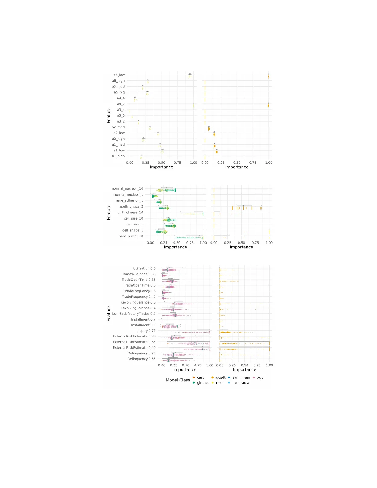
CASHomon Sets: Eﬃcien t Rashomon Sets A cross Multiple Mo del Classes and their Hyp erparameters Fiona Katharina Ew ald ⋆ 1 , 2 [0009 − 0002 − 6372 − 3401] , Martin Binder ⋆ 1 , 2 , Bernd Bisc hl 1 , 2 [0000 − 0001 − 6002 − 6980] , Matthias F eurer 3 , 4 [0000 − 0001 − 9611 − 8588] , and Giusepp e Casalicc hio 1 , 2 [0000 − 0001 − 5324 − 5966] (  ) 1 Departmen t of Statistics, LMU Munich, Munic h, Germany  Giuseppe.Casalicchio@stat.uni-muenchen.de 2 Munic h Cen ter for Mac hine Learning (MCML), Munich, German y 3 TU Dortmund Univ ersity , Dortm und, Germany 4 Lamarr Institute for Machine Learning and Artiﬁcial In telligence, Dortmund, German y Abstract. Rashomon sets are mo del sets within one mo del class that p erform nearly as well as a reference mo del from the same mo del class. They rev eal the existence of alternative well-performing mo dels, which ma y supp ort diﬀeren t in terpretations. This enables selecting mo dels that matc h domain kno wledge, hidden constrain ts, or user preferences. How- ev er, eﬃcient construction metho ds curren tly exist for only a few model classes. Applied machine learning usually searches many mo del classes, and the b est class is unkno wn b eforehand. W e therefore study Rashomon sets in the combined algorithm selection and hyperparameter optimiza- tion (CASH) setting and call them CASHomon sets . W e prop ose Tr u- V aRImp , a mo del-based active learning algorithm for lev el set estima- tion with an implicit threshold, and provide con vergence guaran tees. On syn thetic and real-w orld datasets, Tr uV aRImp reliably iden tiﬁes CASHomon set mem b ers and matc hes or outp erforms naive sampling, Ba yesian optimization, classical and implicit lev el set estimation meth- o ds, and other baselines. Our analyses of predictiv e multiplicit y and feature-imp ortance v ariabilit y across mo del classes question the common practice of interpreting data through a single model class. Keyw ords: Rashomon Eﬀect · Level-set Estimation · F eature Impor- tance · Predictive Multiplicit y · Automated Machine Learning 1 In tro duction The R ashomon eﬀe ct [5] refers to the existence of multiple mo dels with compara- ble predictiv e p erformance that capture diﬀerent asp ects of the data. Serving as a foundational to ol for systematically studying this eﬀect, a R ashomon set [12] ⋆ Equal contribution 2 F. K. Ewald, M. Binder et al. is a set of mo dels that perform almost as w ell as a reference mo del. Recently , Rudin et al. [27] emphasized its practical yet underestimated imp ortance in ap- plied machine le arning (ML), noting its implications and impact on (1) users’ ﬂexibilit y in selecting mo dels based on domain kno wledge or preferences, such as fairness constrain ts; (2) the uncertain ty of mo del-based summary statistics; and (3) the reliability of explanations in interpr etable machine le arning (IML). Unfortunately , eﬃcien t Rashomon set construction is currently possible for only a few mo del classes. Y et diﬀeren t model classes are suited for diﬀeren t problems, and the b est class is rarely kno wn in adv ance [10, 29, 24]. Hyp erp ar ameter op- timization (HPO, [2]) and automate d ML (AutoML, [30, 11, 18]) address this via data-driven model selection. But this often increases complexity: AutoML systems, in their main and somewhat exclusive pursuit of maximizing predictiv e p erformance, select ﬂexible, non-parametric models or ensembles, often ignoring in terpretability and other constraints. As a result, the models pro duced by an AutoML system are typically complex and diﬃcult to understand. T o address this gap, w e contribute the following: (1) W e formally introduce CASHomon sets (Section 3), whic h extend Rashomon sets beyond a single mo del class in the c ombine d algorithm sele ction and hyp erp ar ameter optimization (CASH) setting. (2) W e in tro duce Tr uV aRImp , a model-based activ e learning algorithm for level set estimation (LSE) with an implicitly deﬁned threshold (Section 4), whic h can b e view ed as a Ba y esian optimization algorithm, and pro vide theoretical accuracy guaran tees. (3) W e empirically show that TruV aRImp eﬃciently ﬁnds CASHomon sets and p erforms comp etitiv ely with, or b etter than, naiv e sampling, AutoML-based pip elines, and other LSE baselines on nine datasets (Section 5). (4) W e further study CASHomon sets from an application p erspective (Sec- tion 5.3), ﬁnding that predictiv e m ultiplicity , quantiﬁed b y Rashomon capac- it y [16], which we extend to regression tasks, can diﬀer b et ween Rashomon and CASHomon sets, and that fe atur e imp ortanc e (FI) v alues can v ary sub- stan tially across mo del classes, questioning the common practice of basing in terpretations on a single mo del class. 2 Related W ork W e p osition our w ork at the intersection of (i) Rashomon sets for predictiv e m ultiplicity and in terpretability , and (ii) LSE for eﬃcient identiﬁcation of near- optimal regions in hyp erp ar ameter (HP) spaces. R ashomon eﬀe ct in interpr etability and pr e dictive multiplicity. Prior work shows that Rashomon sets often con tain mo dels with desirable prop erties (e.g., inter- pretabilit y or fairness) without substantial p erformance loss [28, 27]. Rashomon- based analyses hav e also been used to study predictiv e m ultiplicity and the insta- bilit y of explanations (e.g., feature importance) derived from predictive mo dels CASHomon Sets 3 [17, 15, 25, 19]. W e analyze both asp ects: we study predictive multiplicit y us- ing the R ashomon c ap acity [16] and the v ariabilit y of feature imp ortance across w ell-p erforming mo dels using variable imp ortanc e clouds (VICs, [9]). Ho wev er, many existing works on Rashomon sets either study them theoret- ically or develop construction or exploration metho ds for sp eciﬁc mo del classes. Examples include ridge regression and related linear-model settings [9, 28], sparse GAMs [32], rule lists [23], rule sets [8], neural netw orks through drop out-based exploration [17], gradient bo osting [15], and for additive mo dels, kernel ridge regression, and random forests [20]. F or generalized and scalable optimal sparse decision trees (GOSDT) [22], a prominen t approach to construct a Rashomon set is TreeF ARMS [31], whic h we use as a baseline in our empirical comparison (Section 5). Another line of w ork uses candidate mo dels generated b y AutoML systems (e.g., H2O AutoML [21]) as a pro xy Rashomon set that includes m ulti- ple mo del classes and studies the v ariabilit y of explanations [7]. How ever, these approac hes either remain tied to a sp eciﬁc mo del class or rely on ﬁrst gener- ating a large p ool of candidate mo dels and then subsetting it retrosp ectiv ely , rather than directly identifying suc h sets during searc h. In contrast, we formal- ize Rashomon sets directly in the CASH setting, where the mo del class itself is part of the search space, and propose an eﬃcient algorithm for identifying candidate mo dels across heterogeneous mo del classes. L evel set estimation and hyp erp ar ameter optimization. LSE 5 [14] identiﬁes the set of inputs for whic h an unknown function is ab o ve or b elo w a given threshold. W e frame CASHomon set construction as LSE, where candidates are classiﬁed b y whether p erformance lies within a tolerance of the optimum. Since characterizing suc h sets o ver a contin uous domain is usually infeasible, LSE metho ds classify a ﬁnite candidate subset. This diﬀers from standard hyperparameter optimization (HPO), whic h targets one near-optimal conﬁguration. Bry an et al. [6] studied activ e LSE for expensive blac k-b o x functions us- ing Gaussian processes (GPs) [26]. Their str add le heuristic samples where the threshold lie s within the conﬁdence region of the function v alue and prioritizes p oin ts where the distance b et ween the conﬁdence region bounds and the thresh- old v alue is largest. Gotov os et al. [14] reﬁned this b y intersecting conﬁdence regions across iterations and discarding p oin ts once the intersection no longer crosses the threshold. Crucially , they also prop ose implicitly deﬁne d thresholds relativ e to the unkno wn optimum. This maps directly to ﬁnding CASHomon sets (and Rashomon sets) when the best mo del serves as a reference but is unknown. Boguno vic et al. [3] propose TruV aR , an LSE algorithm that handles p oin twise ev aluation costs and heteroscedastic noise. Instead of sampling only by conﬁ- dence width, TruV aR selects points that most reduce conﬁdence widths for all p oin ts not y et classiﬁed to below a shrinking target v alue. Among GP-based LSE metho ds, Tr uV aR is the most direct methodological precursor to our ap- proac h. W e extend Tr uV aR to implicit thresholds using the method of Gotov os 5 While Gotov os et al. [14] also call their algorithm “LSE”, w e use the term for the general problem and denote their algorithm in monospace fon t, LSE . 4 F. K. Ewald, M. Binder et al. et al. [14] in Tr uV aRImp (Section 4). Concretely , TruV aRImp jointly trac ks p oten tial minimizers and threshold-uncertain p oin ts, then allo cates ev aluations to reduce uncertain ty in b oth sets. 3 F ormalization of CASHomon Sets Let I : D × Λ → H b e an induc er which maps data D ∼ ( P X Y ) and a hyp erp ar am- eter c onﬁgur ation (HPC) λ ∈ Λ to a ﬁtted mo del f : X → R g , where g equals 1 for regression and the num b er of classes for classiﬁcation. The i -th observ ation in D is  x ( i ) , y ( i )  , i ∈ { 1 , ..., n } , and the set of all datasets is D = S n ∈ N ( X × Y ) n , where X is the feature space and Y is the target space. Let L : Y × R g → R , be a p oint wise loss function and R ( f ) = E ( x ,y ) ∼ P X Y [ L ( y , f ( x ))] b e the exp ected risk, appro ximated via the empirical risk R emp ( f ) = 1 n P n i =1 L ( y ( i ) , f ( x ( i ) )) . 3.1 Bac kground on CASH In the abov e formalism, HPs can represent all decisions made when pro duc- ing a model (or p otentially a full ML pip eline). This can include, in partic- ular, c ho osing and parameterizing data prepro cessing, selecting features, and c ho osing a learning algorithm. Letting categorical HPs represen t discrete al- gorithmic decisions (i.e., which metho d to select) is a common wa y to reduce the CASH problem to an HPO problem [30, 11]. This w ork concen trates on join t optimization of the mo del class and its asso ciated HPs. W e use the term mo del class to refer to the set of mo dels H m := range( I m ) pro duced by the same inducer I m with HP space Λ m . Th us, this captures the intuition that a mo del class is a set of models that share a common structure, e.g., linear mo dels (LMs), decision trees (DT s), or neural net works (NNs). W e generally ha ve multiple d iﬀeren t mo del classes, indexed by m ∈ { 1 , . . . , M } . W e can no w consider the ov erall mo deling pro cess as a single inducer, which is conﬁgured sim ultaneously b y m and λ m , where the latter is sub ordinate to the former (i.e., a t ypical hierarchical HPC structure, commonly encountered in CASH): I CASH ( D , ( m, λ m )) = I m ( D , λ m ) with Λ CASH := S M m =1 { ( m, λ m ) | λ m ∈ Λ m } as the corresp onding HP space. W e denote the union of all mo del classes as the CASH hyp othesis sp ac e H CASH := S M m =1 H m , i.e., the set of all mo dels that can b e pro duced by the ov erall mo deling pro cess when any one of the M mo del classes can b e used. 3.2 F rom Rashomon Sets to CASHomon Sets A Rashomon set is a set of measurable functions from X to R g con taining mo d- els that p erform nearly equally well as a reference model f ref [12]. F ormally , RS ( ε, f ref , F ) := { f ∈ F | R ( f ) ≤ R ( f ref ) + ε } , where the oﬀset ε > 0 can ei- ther b e giv en in absolute terms, or as a v alue relative to R ( f ref ) ; in general, we write ε = ε abs + ε rel R ( f ref ) , assuming R ( f ref ) > 0 . In practice, f ref is t ypically estimated as the empirical risk minimizer from the considered hypothesis space, CASHomon Sets 5 yielding the empiric al R ashomon set . Prior work restricts F to a sp eciﬁc mo del class to mak e the Rashomon set estimation feasible (see Section 2). Instead, we do not restrict F to a single model class and approximate F by the set of mo dels pro duced when ﬁtting a mo del to the given dataset and v arying its HPs. F or a single mo del class with inducer I m and HP space Λ m , w e sp ecify the set of mo dels F obtainable by tuning λ m for a giv en dataset D ∈ D as F = H D m, HPO := range( I m ( D , · )) = {I m ( D , λ m ) | λ m ∈ Λ m } . (1) As a necessary consequence of restricting the function class to H D m, HPO , the HPO R ashomon set RS ( ε, f ref , H D m, HPO ) is generally a strict subset of RS ( ε, f ref , H m ) . W e further discuss this restriction and the impact of ha ving only ﬁnite data in App endix A. The size of this HPO Rashomon set generally increases with the n umber of HPs that I m has, and, therefore, naturally lends itself to b e com bined with the CASH approach (Section 3.1). So while using H D m, HPO instead of H m is a restriction, our approach also allo ws for a larger and more diverse Rashomon set b y considering m ultiple mo del classes at the same time when using the CASH searc h space. W e deﬁne the CASHomon set as C S ( ε, f ref , H D CASH ) :=  f ∈ H D CASH | R ( f ) ≤ R ( f ref ) + ε  , where H D CASH := S M m =1 {I m ( D , λ m ) | λ m ∈ Λ m } . When the dataset D is ﬁxed, w e say that an HPC λ m ∈ Λ m is in the Rashomon set if, for m ∈ { 1 , . . . , M } , I m ( D , λ m ) is in the Rashomon set. Although M mo del classes are considered in H D CASH , not all of them will b e represented in the CASHomon set if some mo del classes outp erform others, i.e., mo del class selection is p erformed on the ﬂy . Due to the computational complexit y of ﬁnding a compact description of the exact CASHomon set, w e approximate it using a random subsample of mo dels inside that set, which is suﬃcient for analysis methods that op erate on dis- crete Rashomon sets or require integration ov er them. This aligns with the lit- erature, where Rashomon sets are often appro ximated b y sampling from them (e.g., [15, 17]). Given D and a prop osal distribution P CASH on Λ CASH , our goal is to sample from the CASHomon set through rejection sampling: (1) Sample a candidate set of size C , ˜ Λ = { λ i } C i =1 ∼ ( P CASH ) C ; (2) Ev aluate or pre- dict the (empirical) risk R emp ( I ( D , λ i )) for all i ; (3) Accept all λ i for whic h R emp ( I ( D , λ i )) ≤ R emp ( f ref ) + ε and reject all others. Aiming for a represen ta- tiv e sample from P CASH ( λ | I ( D , λ ) ∈ C S ) is a natural goal for c haracterizing C S as o ver- or undersampling particular regions could distort downstream analyses. 4 An Eﬃcient Algorithm for Finding CASHomon Sets Algorithmically , deciding which mo dels are in the CASHomon set reduces, in principle, to an expensive, blac k-b o x level-set estimation problem, p ossibly on a mixed and hierarchical space. Direct application of LSE pro cedures (using appropriate surrogate models due to their computational cost and the complex searc h-space structure) is complicated by the fact that the level-set threshold 6 F. K. Ewald, M. Binder et al. is in our case only implicitly deﬁned [14] as R ( f ref ) + ε , where f ref is the b est p erforming mo del from H D CASH , which also needs to b e estimated. While one could ﬁrst p erform HPO to iden tify a reference model, follow ed by a (surrogate- based) LSE algorithm to iden tify mo dels in the CASHomon set, we introduce an algorithm that com bines these steps, yielding greater eﬃciency . W e prop ose the TruV aRImp algorithm, which extends the Tr uV aR algo- rithm [3] to handle implicitly deﬁned threshold levels. F or (direct, explicit) LSE, Tr uV aR maintains a ﬁnite set of candidate p oin ts to classify as lying ab o ve or b elo w the given threshold. It uses a GP mo del that predicts both the p osterior mean µ ( λ ) and the p osterior v ariance σ 2 ( λ ) of the ob jectiv e v alue at each can- didate p oint λ . In each iteration t , candidates with p osterior distributions that fall to one side of the threshold with high conﬁdence are classiﬁed and remov ed from the active, unclassiﬁed set U t and instead added to the high set H t or the lo w set L t . 6 Tr uV aR pro ceeds in ep o chs i , which often last for multiple itera- tions, and whic h ha ve a corresp onding target conﬁdence b ound η ( i ) . This v alue shrinks according to η ( i +1) = r η ( i ) as ep o c hs adv ance, where the reduction fac- tor r ∈ (0 , 1) is a conﬁguration parameter. It chooses which candidate p oin ts λ to ev aluate based on the summed reduction of the current uncertaint y estimate β 1 / 2 ( i ) σ ( λ ′ ) across all unclassiﬁed candidates λ ′ ∈ U t , where we clip the reduction at uncertaint y η ( i ) . The algorithm allows this reduction to b e scaled b y a (user- deﬁned) cost function cost( λ ) , and β ( i ) is an epo c h-dep enden t scaling factor. The ep och adv ances once all points in U t ha ve conﬁdence b elo w (1 + δ ) η ( i ) , with conﬁgurable slac k parameter δ > 0 . Boguno vic et al. [3] present tw o v ariants of their algorithm: One for LSE, as explained abov e, in which unclassiﬁed p oin ts U t are categorized in to H t and L t , and one for optimization, where points are classiﬁed based on whether they are p oten tial risk minimizers. Tr uV aRImp extends TruV aR for LSE with an implicitly deﬁned threshold. Its underlying idea is to sim ultaneously track a set of p oten tial minimizers M t and a set of points U t that are unclassiﬁed with respect to the implicit threshold, thereb y using b oth v ariants of TruV aR in one. One approac h to tracking minimizers and level sets simultaneously was presen ted by Goto vos et al. [14]; ho wev er, our algorithm selects points to ev aluate in a manner similar to Tr uV aR , based on which point reduces the p osterior conﬁdence to a giv en threshold the most. 4.1 Our T ruV aRImp Algorithm F ollo wing Bogunovic et al. [3], w e mo del the ob jective function c ( λ ) : ˜ Λ → R as a GP with constant mean µ 0 = 0 , kernel function k ( λ, λ ′ ) and, in general, heteroscedastic measurement noise ϵ ( λ ) ∼ N (0 , σ 2 ( λ )) , where we observe noisy ob jective v alues ˆ c = c ( λ ) + ϵ ( λ ) . W e use the k ernel matrix K t =  k ( λ i , λ j )  t i,j =1 for p oin ts { λ i } t i =1 observ ed un til after iteration t , the white noise term Σ t = diag( σ 2 ( λ 1 ) , . . . , σ 2 ( λ t )) , and the cross-co v ariance v ector k t ( λ ) = [ k ( λ i , λ )] t i =1 . 6 W e use a notation to describ e Tr uV aR that diﬀers sligh tly from the one used in [3]. CASHomon Sets 7 The p osterior distribution of c ( λ t +1 ) given the vector of the ﬁrst t observ ations ˆ c 1: t is th us N ( µ ( λ t +1 ) , σ 2 ( λ t +1 )) , where µ t ( λ t +1 ) = k t ( λ t +1 ) ⊤ ( K t + Σ t ) − 1 ˆ c 1: t (2) σ 2 t ( λ t +1 ) = k ( λ t +1 , λ t +1 ) − k t ( λ t +1 ) ⊤ ( K t + Σ t ) − 1 k t ( λ t +1 ) . (3) Similar to Bogunovic et al. [3], for some λ ′ ∈ ˜ Λ w e denote the p osterior v ariance of c ( λ ′ ) given observ ations at λ 1 , . . . , λ t − 1 as well as an additional observ ation at λ as σ 2 t − 1 | λ ( λ ′ ) . This represents a one-step look ahead ev aluation of the p osterior v ariance: Given that the algorithm has already made t − 1 observ ations, this quan tity indicates ho w ev aluating a speciﬁc c hoice of c ( λ ) will inﬂuence the p osterior v ariance at another p oin t λ ′ . Notably , σ 2 t − 1 | λ ( λ ′ ) do es not dep end on the observ ed v alue ˆ c at λ and can b e calculated eﬃciently , as describ ed in App endix B of Boguno vic et al. [3]. Algorithm 1 shows our TruV aRImp algorithm. It chooses where to ev aluate the ob jective, so that p oin ts from a ﬁnite input set ˜ Λ are eﬃciently classiﬁed as ab o v e or below a threshold level h . Without loss of generality , we consider the case of minimization, i.e., ﬁnding a CASHomon set with a threshold deﬁned in terms of the (unkno wn) minim um of the ob jective function: c min = min λ ∈ ˜ Λ c ( λ ) . W e set h = c min × (1+ ε rel )+ ε abs , where we allow the expression of the CASHomon set in terms of relative ( ε rel ≥ 0 ; assuming ∀ λ : c ( λ ) ≥ 0 ) or absolute ( ε abs ≥ 0 ) oﬀset from the minimum. Typically , one of these is zero; we include b oth v ariables in this form ula to remain general. Tr uV aRImp k eeps trac k of a set of p oten tial minimizers M t of c ( · ) , a set of candidate points L t classiﬁed as below the threshold, a set of p oin ts classiﬁed as ab o ve the threshold H t , and a set of p oin ts unclassiﬁed with resp ect to the threshold U t . L t , U t and H t form a partition of ˜ Λ , and M t ⊆ U t ∪ L t . F or each p oin t, the algorithm calculates conﬁdence in terv als [ l t ( λ ) , u t ( λ )] = [ µ t ( λ ) − β 1 / 2 ( i ) σ t ( λ ) , µ t ( λ ) + β 1 / 2 ( i ) σ t ( λ )] . (4) It works under the assumption that, if β ( i ) is chosen large enough, the true c ( λ ) is in [ l t ( λ ) , u t ( λ )] with high probability . A point λ is therefore remov ed from M t whenev er its conﬁdence in terv al does not ov erlap with the p essimistic estimate of the minimum c pes min ,t = min λ ′ ∈ M t − 1 u t ( λ ′ ) , and a p oin t is remo ved from U t and added to either L t or H t whenev er its conﬁdence in terv al does not ov erlap with the range of p ossible threshold v alues [ h opt t , h pes t ] (see Algorithm 1, lines 9 – 8). Lik e TruV aR , Tr uV aRImp pro ceeds in epo chs, which count up whenever con- ﬁdence interv als for all remaining candidates in U t and M t fall b elo w a threshold prop ortional to η ( i ) (Algorithm 1, line 25). Figure 1 shows the main comp onen ts of the algorithm at iteration t . Our theoretical analysis (App endix D) shows that, with suitably chosen algorithm parameters, this approach iden tiﬁes p oin ts in the CASHomon set up to a giv en accuracy ϵ with high probability . 8 F. K. Ewald, M. Binder et al. Algorithm 1 T runcated V ariance Reduction for Implicitly Deﬁned LSE ( Tr uV aRImp ) Input: Ob jectiv e function c ( · ) ; Domain ˜ Λ ; ev aluation-cost function cost( λ ) ; GP prior ( µ 0 , σ ( λ ) ; k ( x , x ′ ) ); conﬁdence b ounding parameters δ > 0 , r ∈ (0 , 1) , { β ( i ) } i ≥ 1 , η (1) > 0 ; ε rel ≥ 0 , ε abs ≥ 0 Output: Sets ( L, H, U ) predicted to b e resp ectiv ely b elow, abov e and unclassiﬁed with resp ect to the implicit threshold h = min λ ∈ ˜ Λ c ( λ ) × (1 + ε rel ) + ε abs 1: Initialize L 0 = H 0 = ∅ , M 0 = U 0 = ˜ Λ , ep och n umber i = 1 2: for t = 1 , 2 , . . . do 3: Letting ∆ i ( D , σ 2 , p ) := P λ ′ ∈ D max  p 2 β ( i ) σ 2 ( λ ′ ) − η 2 ( i ) , 0  , 4: ﬁnd λ t ← arg max λ ∈ ˜ Λ nh ∆ i ( U t − 1 , σ 2 t − 1 , 1) − ∆ i ( U t − 1 , σ 2 t − 1 | λ , 1)+ ∆ i ( M t − 1 , σ 2 t − 1 , 1+ ε rel ) − ∆ i ( M t − 1 , σ 2 t − 1 | λ , 1+ ε rel ) i. cost( λ ) o 5: Ev aluate ob jective at λ t , observe noisy ˆ c t . 6: Calculate µ t and σ t according to (2)–(3), and l t ( λ ) and u t ( λ ) according to (4) 7: c pes min ,t ← min λ ′ ∈ M t − 1 u t ( λ ′ ) 8: h pes t ← c pes min ,t × (1 + ε rel ) + ε abs 9: h opt t ← min λ ′ ∈ M t − 1 l t ( λ ′ ) × (1 + ε rel ) + ε abs 10: H t ← H t − 1 , L t ← L t − 1 , U t ← ∅ , M t ← ∅ 11: for each λ ∈ U t − 1 do 12: if u t ( λ ) ≤ h opt t then 13: L t ← L t ∪ { λ } 14: else if l t ( λ ) > h pes t then 15: H t ← H t ∪ { λ } 16: else 17: U t ← U t ∪ { λ } 18: end if 19: end for 20: for each λ ∈ M t − 1 do 21: if l t ( λ ) ≤ c pes min ,t then 22: M t ← M t ∪ { λ } 23: end if 24: end for 25: while max λ ∈ U t β 1 / 2 ( i ) σ t ( λ ) ≤ (1 + δ ) η ( i ) and max λ ∈ M t β 1 / 2 ( i ) σ t ( λ ) ≤ 1+ δ 1+ ε rel η ( i ) do 26: i ← i + 1 , η ( i ) ← r × η ( i − 1) . 27: end while 28: if budget is exhausted then 29: return H ← H t , L ← L t , U ← U t 30: end if 31: end for Implementation Notes. In practice, the GP’s kernel HPs are usually unkno wn and estimated from observ ed p erformance data. In applications such as HPO, they are re-ﬁt in eac h iteration, so a diﬀerent kernel function is used at each step. W e calculate σ 2 t − 1 | λ ( λ ′ ) from the kernel function at t − 1 to make use of the CASHomon Sets 9 eﬃciency gains mentioned ab o ve, but it ceases to be the exact v alue of σ 2 t ( λ ′ ) for λ = λ t . This is a common simpliﬁcation; as seen in Section 5, the algorithm w orks well in practice. F urthermore, the CASH hyperparameter space Λ CASH is generally hierarc hi- cal: the HPs of inducer I m are activ e only when model class m is selected. Al- though one could design problem-sp eciﬁc kernels that transfer information across mo del classes, we mak e the problem-agnostic assumption that p erformance ob- serv ations are informativ e only within the same model class. This yields the blo c k-diagonal k ernel k ( λ m , λ ′ m ′ ) = δ mm ′ k m ( λ m , λ ′ m ) with indep endent class- sp eciﬁc kernels k m ( · , · ) deﬁned on eac h subspace Λ m . Minimum Upper Bound ( c min,t pes ) Minimum Lower Bound Confidence Region [ l t ( λ ) , u t ( λ )] M t Target Confidence ( η ( i ) ) Potential Minimizers ( M t ) Threshold Upper Bound ( h t pes ) Threshold Lower Bound ( h t opt ) True Threshold ( h ) Min. × ( 1 + ε rel ) Unclassified ( U t ) U t Target Confidence ( η ( i ) ) 0 1 2 3 0.0 0.2 0.4 0.6 0.8 1.0 Fig. 1: Illustration of the TruV aRImp algorithm. The true (unkno wn) function is sho wn in green, with known function v alues c ( λ ) as blac k dots, through which a GP mo del is ﬁt (purple line with transparen t conﬁdence region). M t is the set of potential minimizers (purple strip at the b ottom), for which the conﬁdence in terv al crosses the “p essimistic” (i.e., highest p ossible within conﬁdence region) minim um c pes min ,t (upp er red dashed line). Conﬁguration p oin ts λ are classiﬁed as b elonging to the low er or upp er set ( L t and H t , not shown), or remain unclassiﬁed ( U t , blue strip at the bottom), dep ending on whether their conﬁdence interv al crosses the region of plausible threshold v alues [ h opt t , h pes t ] (blue dashed lines). In this illustration, these are relativ e to the minimum with ε rel = 2 , ε abs = 0 . Tr uV aRImp selects points based on ho w m uch ev aluating them will reduce the v ariance for candidates in b oth M t and U t that goes b eyond their target conﬁdence v alues η ( i ) the most (green and purple ribb ons around the GP mean). 5 Exp erimen ts W e (1) ev aluate the reliability and eﬃciency of TruV aRImp , and (2) e mpiri- cally examine practical implications of extending Rashomon sets to the CASH 10 F. K. Ewald, M. Binder et al. h yp othesis space. T o address (1), we compare our prop osed TruV aRImp al- gorithm against LSE baselines, HPO, and random ev aluation in Section 5.2, addressing our ﬁrst t wo research questions (R Qs): R Q 1.1 Can TruV aRImp ﬁnd the CASHomon set accurately and eﬃciently? R Q 1.2 How does TruV aRImp p erform in comparison to baselines? Regarding (2), we explore the mo dels in the CASHomon sets found by Tr u- V aRImp , considering the following questions in Section 5.3: R Q 2.1 Do Rashomon and CASHomon mo dels diﬀer in predictive p erformance? R Q 2.2 Do Rashomon and CASHomon sets diﬀer in predictive m ultiplicity? R Q 2.3 How do FI v alues v ary across Rashomon and CASHomon mo dels? The co de and repro duction scripts are a v ailable at: https://github.com/slds- lmu/paper_2024_rashomon_set . 5.1 Exp erimen tal Setup T o study CASHomon sets in a large, diverse search space, we use mo del classes that are commonly used in practice and that also v ary in interpretabilit y . W e ev aluate DT s ﬁtted using the CAR T algorithm ( cart ) and GOSDT ( gosdt ). W e also use gradient b oosting models ( xgb ), feedforw ard NNs ( nnet ), supp ort v ector mac hines ( svm ) with t wo kernels ( linear and radial ), and elastic nets ( glmnet ); the latter as an LM for regression and a logistic mo del for classiﬁcation datasets. The HP searc h spaces are mostly lifted from [1] and are listed in App endix C. W e fo cus on datasets used by Xin et al. [31] and their proposed binarization for comparability . W e consider v arious classiﬁcation tasks: COMP AS ( CS , with and without binarization), German Cr e dit ( GC ), and binarized versions of c ar evaluation ( CR ), Monk 2 ( MK ), br e ast c anc er ( BC ), and FICO ( FC ). W e also in- clude tw o regression tasks: Bike Sharing ( BS ) and a syn thetic dataset ( ST ). See App endix B for more details on the datasets. W e split each dataset in to tw o parts. W e use 2/3 for mo del selection, where w e estimate R emp using a 10 × 10 -fold rep eated cross-v alidation, and then reﬁt ﬁnal mo dels on the full training split. W e use the remaining 1/3 of the data as test data for p erformance, predictive multiplicit y , and FI analysis. T o compute CASHomon sets, w e sample 8000 HPCs uniformly at random from the searc h space of eac h learning algorithm as the candidate set ˜ Λ . W e ev aluate eac h HPC on each dataset, measuring the Brier score for classiﬁcation and the ro ot mean squared error (RMSE) for regression tasks. gosdt can handle only binary data and is therefore ev aluated only on our binarized classiﬁcation datasets. F or a giv en task, w e consider the b est HPC found ov er all considered model classes as the reference mo del f ref and use its performance to determine the CASHomon set cutoﬀ using commonly used [25, 7] v alues ε rel = 0 . 05 and ε abs = 0 . 5.2 Exp erimen ts on Lev el Set Estimation W e ev aluate the abilit y of TruV aRImp to identify the CASHomon set, treat- ing the LSE problem as an active learning problem: conﬁguration points are CASHomon Sets 11 selected and ev aluated so that a surrogate model ﬁtted to the observ ed design p oin ts can b e used to classify whether unobserved conﬁgurations b elong to the CASHomon set. This viewp oin t is reﬂected in the acquisition strategy of Tr u- V aRImp , whic h prioritizes ev aluations that reduce uncertain ty ab out the mem- b ership of curren tly unclassiﬁed p oints. It is also aligned with the goal stated at the end of Section 3.2, namely to sample from the conditional distribution P CASH ( λ | I ( D , λ ) ∈ C S ) , if the candidate set is itself sampled from P CASH and the surrogate predicts p erformance v alues reasonably well. There are diﬀeren t wa ys to use a GP surrogate to predict the CASHomon set. A fully Ba yesian ev aluation could av erage CASHomon set mem b ership ov er p osterior GP samples: In eac h GP sample, the reference conﬁguration and cutoﬀ v alue would, in general, diﬀer, and the uncertaint y ab out the true best mo del w ould b e eﬀectiv ely marginalized ov er. How ever, this would not reﬂect actual practice, where researc hers care ab out generating alternativ e models and expla- nations for a concrete, ﬁtted reference model. Therefore, w e tak e an application- cen tric view, ev aluating a TruV aRImp run based on the CASHomon set it would generate from the best observe d model. W e run Tr uV aRImp with ob jective ˆ c ( λ ) = R emp ( I ( D , λ )) . After t ev aluations, we use the incumbent f ( t ) ref = I ( D , ˆ λ ∗ t ) with ˆ λ ∗ t ∈ arg min λ ∈{ λ 1 , ··· ,λ t } ˆ c ( λ ) as reference model. The corresp onding cutoﬀ ˆ h t = (1 + ε rel ) R emp ( f ( t ) ref ) + ε abs is then used to classify conﬁgurations into the pre- dicted CASHomon set based on mo del predictions, ˆ C S t = { λ ∈ ˜ Λ | µ t ( λ ) ≤ ˆ h t } . W e compare this against the (ﬁnite) ground truth sample from the (inﬁnite) CASHomon set, calculated as a subset of ˜ Λ using the precomputed ˆ c ( λ ) with the minimum ov er ˜ Λ as reference, as this is the represen tative sample from the CASHomon set that a practitioner would obtain by ev aluating all samples in ˜ Λ . W e compare TruV aRImp against the following LSE algorithms: STRADDLE [6], LSE and LSE IMP (the level set estimation algorithm and its implicit LSE v arian t in tro duced b y Goto vos et al. [14]), and the original Tr uV aR algorithm [3]. W e furthermore consider RANDOM (random conﬁguration p oin t ev aluations), and OPTIMIZE : HPO via Bay esian optimization, using the exp ected improv ement ac- quisition function [13]. By comparing our LSE-based approach with a Ba yesian optimization approach on the same CASH space, we implicitly compare against Ca vus et al. [7], who extract their Rashomon set from the archiv e of a standard AutoML system (H2O AutoML [21]) without explicitly targeting the underlying LSE deﬁnition or ev aluating what they lose b y disregarding this (they eﬀectively tak e the best mo dels from the underlying random search of H2O AutoML). See App endix E.1 for more details on algorithm conﬁguration parameters. W e use a candidate set of 8000 pre-computed p erformance v alues per mo del class; the CASH space th us has 48,000 candidates in total for binary datasets, 40,000 for the others. Figures 2 and 6 (Appendix E.1) show progress in surro- gate model quality , which we quan tify using the F1 score, since CASHomon set mem b ership is a highly imbalanced binary classiﬁcation problem. On a verage, Tr uV aRImp outp erforms baselines in classifying CASHomon set members, en- abling accurate threshold decisions. Notably , the CASHomon set task app ears 12 F. K. Ewald, M. Binder et al. diﬃcult for baselines, likely b ecause the search space is complex and multimodal. MEAN BS ST 0 200 400 600 0 200 400 600 0 200 400 600 0.4 0.6 0.8 LSE Iteration Algorithm LSE LSE IMP OPTIMIZE RANDOM STRADDLE TruVar TruVaRImp Fig. 2: Mean CASHomon set algorithm progress in terms of F1 score of the surrogate model predicting CASHomon set mem b ership. The iteration count do es not include the initial sample of 30 p oin ts per model class. The left facet sho ws the mean v alues ov er all datasets. The middle and righ t sho w individual p erformance on tw o example datasets. 5.3 An Application P ersp ectiv e As w e are not aw are of an y algorithm pro ducing Rashomon sets across diverse mo del classes, we compare our CASHomon sets with Rashomon sets found b y a state-of-the-art Rashomon set algorithm, namely TreeF ARMS [31], which is a p opular, ready-to-use metho d for ﬁnding Rashomon sets for GOSDT [22]. W e illustrate that p erformance, predictiv e multiplicit y , and FI v alues may dif- fer b et w een mo dels from the TreeF ARMS Rashomon set and the CASHomon sets. F or the latter, we use the results from running TruV aRImp on the can- didate set, i.e., HPCs actually ev aluated by Tr uV aRImp , and ﬁt the resulting conﬁgurations on the training split of eac h dataset. Pr e dictive Performanc e. The top ro w of Figure 3 shows the Brier score distribu- tions on the test set for three represen tative tasks ( BC , CR , and binarized CS ). The reference mo dels of Rashomon and CASHomon sets diﬀer notably , since mo dels from the mo del class gosdt often p erform comparably worse than some of the other mo del classes. Only the CASHomon set of CS con tains gosdt mo dels; for BC and CR , tree-based mo dels do not perform w ell enough. 7 Hence, mo dels in our CASHomon sets p erform, on av erage, b etter than those found by TreeF ARMS . F or b etter reference mo dels, ε rel R ( f ref ) b ecomes smaller, and p erformance tends to scatter less across mo dels, even on a test set, as seen for BC and CR . 7 T able 8, Appendix E, shows the num b er of mo dels per mo del class contained in the CASHomon sets p er dataset. CASHomon Sets 13 (a) T ask BC (b) T ask CR (c) T ask CS (binarized) Fig. 3: T est p erformance and R C for tasks BC, CR, and CS (binarized) across the TreeF ARMS Rashomon set and our CASHomon set. T op row: Brier score dis- tributions. Bottom row: RC (y-axis) v ersus Brier score (x-axis); horizontal b o x- plots summarize test score distributions; triangles indicate the reference mo del. Pr e dictive Multiplicity. T o analyze predictive multiplicit y , we consider R ashomon c ap acity (RC, [16, 17]), which measures the spread in predictions across mo dels within a Rashomon set. 8 It is non-trivial to trade oﬀ or compare RC v ersus predictiv e p erformance in ev aluation. On the one hand, since our goal is to assess predictiv e multiplicit y of near-optimal mo dels, we aim to ﬁnd Rashomon or CASHomon sets with higher RC while achieving go od predictive p erformance. On the other hand, we exp ect that mo del sets con taining less w ell-generalizing mo dels hav e a higher RC. What w e can certainly say is this: (1) Not detecting what the optimal prediction mo del and its performance are, seems problematic. (2) Assuming (1) is well-appro ximated, we w ant to know how m uch v ariabilit y exists across the space of all admissible mo dels. The bottom ro w of Figure 3 plots the R C against the test p erformances for the TreeF ARMS Rashomon set and our CASHomon set. The triangles indicate the reference mo del in each set. Across all considered datasets, there is a tendency for the TreeF ARMS Rashomon set to yield higher R C v alues than our CASHomon sets, how ev er, at the cost of a higher Brier score. W e also observe that the reference mo dels in the TreeF ARMS Rashomon sets p erform w orse on the test data than the ones in our CASHomon sets, esp ecially when comparing the reference mo del’s test p erformance to the remaining models within each set. Notably , in task CS , our CASHomon set not only contains better generalizing mo dels than the TreeF ARMS Rashomon set, but also results in a higher RC. 8 W e slightly adapt the original per-observ ation, classiﬁcation-speciﬁc deﬁnition to measure predictive m ultiplicity across the entire dataset, and extend it to regression problems. The formal deﬁnition and a pseudo code for RC are in App endix E.2. 14 F. K. Ewald, M. Binder et al. Fig. 4: VICs for our CASHomon set (left) and for the TreeF ARMS Rashomon set (right) on task CS . F or each feature, PFI v alues across mo dels are sho wn as a b o xplot together with a p oin t cloud colored by model class, where identical v alues are vertically jittered. PFI v alues are scaled: the maximal PFI v alue for a mo del equals 1. In our CASHomon set, most mo dels are xgb mo dels (178), follo wed by nnet (66) and cart (33) mo dels, but all mo del classes are present. F e atur e Imp ortanc e. Since similarly well-performing mo dels ma y rely diﬀerently on features, we study the FI v alues indu ced by models in the CASHomon set using variable imp ortanc e clouds (VICs, [9]), i.e., sets of FI v ectors, one for eac h mo del in the set. W e quantify mo del reliance via p erm utation feature imp ortance (PFI; [4, 12]), estimated b y av eraging ten p erm utation runs and scaled such that they preserve the within-mo del ranking and relativ e importance of features while enabling comparisons across heterogeneous mo dels and mo del classes. 9 Figure 4 shows the VICs for the binarized CS dataset: the left panel (colored b y mo del class) sho ws our CASHomon set, the righ t shows the TreeF ARMS Rashomon set. In the right panel, v ariation across gosdt mo dels already pro- duces a notable spread in FI v alues, e.g., for priors..3 and priors..0 , the assigned imp ortance v aries across the models from not imp ortant ( 0 ) to most imp ortant ( 1 ). The left panel reveals a second, b et ween-class lay er of v ariation since FI v alues scatter diﬀerently across mo del classes. Moreov er, the t wo mo del sets disagree mark edly on individual features: e.g., for priors..0 , most mo dels in the Rashomon set assign near-zero or near-one imp ortance, whereas mo dels in the CASHomon set show a bulk in [0 . 25 , 0 . 6] . This disagreement reveals that the c hoice of mo del class can substan tially change which features the models rely on most; a pattern we observe across all datasets considered, though the degree of v ariation diﬀers by task (see Appendix E.3). T o the b est of our knowledge, 9 F or formal deﬁnitions of VIC and PFI see App endix E.3. CASHomon Sets 15 a further in terpretation of FI results in a Rashomon context remains an open researc h area b ey ond their utility for mo del selection. 6 Discussion, Limitations and F uture W ork With the CASHomon set, we presen t the ﬁrst formal extension of the Rashomon set across m ultiple mo del classes. Finding CASHomon sets can naturally be framed as an implicit lev el set estimation problem, for which we in tro duce the no vel algorithm TruV aRImp and pro vide conv ergence guaran tees. In con trast to prior w ork, our approach is mo del-class-independent, uniﬁes diﬀerent mo del classes within a single Rashomon set framework, and supp orts eﬃcient search o ver the resulting joint hypothesis space. Our exp erimen ts show that Tru- V aRImp eﬃciently identiﬁes HPCs from the CASHomon set. W e inv estigate v arious prop erties of CASHomon sets, including predictive m ultiplicity using the Rashomon capacit y and FI using VICs. Our analyses rev eal a p ossible trade-oﬀ betw een predictive p erformance and predictive multiplicit y , sho wing that Rashomon set analyses can b e misleading when the set contains p oor predictors. This highlights the imp ortance of constructing Rashomon sets with strong predictiv e p erformance, a goal that may b e harder to ac hieve when the searc h is restricted to a single model class. Moreov er, FI v alues can dif- fer substan tially across mo del classes, implying that explanations derived from a single-class Rashomon set may provide only a partial picture: they may miss imp ortan t explanation v ariability and ma y c hange, once additional, equally com- p etitiv e mo del classes are taken into accoun t. Despite these contributions, sev eral limitations remain and motiv ate future w ork. W e hav e not inv estigated ho w the ε abs and ε rel aﬀect the CASHomon set comp osition; for very small cutoﬀ v alues, the CASHomon set is more likely to only con tain a single model class, and there may b e no vel eﬀects, e.g., higher R C, at larger cutoﬀ v alues where many diﬀerent mo del classes enter the CASHomon set. In particular, in certain scenarios, it might b e preferable to ﬁnd inherently in terpretable models. Curren tly , this is only possible b y restricting TruV aRImp b y pre-selecting certain mo del classes. F uture work could in vestigate other w ays of biasing preferen tially ev aluating more desirable mo del classes, or generally a more div erse set of mo del classes. Finally , w e hav e only started to explore applications of CASHomon sets. The framework allows new analyses of predictive m ultiplicity , mo del selection under ambiguit y , and robustness of FI scores across heterogeneous mo del classes. References 1. Binder, M., Pﬁsterer, F., Bisc hl, B.: Collecting empirical data ab out hyperparam- eters for data driven AutoML. In: ICML W orkshop on AutoML (2020) 2. Bisc hl, B., Binder, M., Lang, M., Pielok, T., Ric hter, J., Co ors, S., Thomas, J., Ullmann, T., Beck er, M., Boulesteix, A., Deng, D., Lindauer, M.: Hyperparameter optimization: F oundations, algorithms, b est practices, and op en c hallenges. Wiley IRDMKD p. e1484 (2023) 16 F. K. Ewald, M. Binder et al. 3. Boguno vic, I., Scarlett, J., Krause, A., Cevher, V.: T runcated v ariance reduction: A uniﬁed approach to Bay esian optimization and level-set estimation. NeurIPS 29 (2016) 4. Breiman, L.: Random forests. MLJ 45 , 5–32 (2001) 5. Breiman, L.: Statistical modeling: The tw o cultures (with comments and a rejoinder b y the author). Stat. Sci. 16 (3) (2001) 6. Bry an, B., Nichol, R.C., Genov ese, C.R., Schneider, J., Miller, C.J., W asserman, L.: A ctive learning for identifying function threshold b oundaries. NeurIPS 18 (2005) 7. Ca vus, M., v an Rijn, J.N., Biecek, P .: Quan tifying mo del uncertaint y with AutoML and Rashomon partial dep endence proﬁles: Enabling trustw orthy and human- cen tered XAI. Inf. Syst. F ront. (2026) 8. Ciap eroni, M., Xiao, H., Gionis, A.: Eﬃcient exploration of the Rashomon set of rule-set mo dels. KDD pp. 478–489 (2024) 9. Dong, J., Rudin, C.: Exploring the cloud of v ariable imp ortance for the set of all go od mo dels. Nat. Mach. In tell. 2 (12), 810–824 (2020) 10. F ernández-Delgado, M., Cernadas, E., Barro, S., Amorim, D.: Do we need hundreds of classiﬁers to solv e real world classiﬁcation problems? JMLR 15 (90), 3133–3181 (2014) 11. F eurer, M., Klein, A., Eggensp erger, K., Springenberg, J., Blum, M., Hutter, F.: Eﬃcien t and robust automated machine learning. NeurIPS pp. 2962–2970 (2015) 12. Fisher, A., Rudin, C., Dominici, F.: All mo dels are wrong, but many are useful: Learning a v ariable’s imp ortance by studying an en tire class of prediction mo dels sim ultaneously . JMLR 20 (177), 1–81 (2019) 13. Garnett, R.: Bay esian optimization. Cambridge Universit y Press (2023) 14. Goto vos, A., Casati, N., Hitz, G., Krause, A.: Activ e learning for level set estima- tion. IJCAI pp. 1344–1350 (2013) 15. Hsu, H., Brugere, I., Sharma, S., Lecue, F., Chen, R.: RashomonGB: Analyzing the Rashomon eﬀect and mitigating predictive multiplicit y in gradient b oosting. NeurIPS 37 , 121265–121303 (2024) 16. Hsu, H., Calmon, F.: Rashomon capacity: A metric for predictive multiplicit y in classiﬁcation. NeurIPS pp. 28988–29000 (2022) 17. Hsu, H., Li, G., Hu, S., et al.: Drop out-based Rashomon set exploration for eﬃcient predictiv e m ultiplicity estimation. arXiv:2402.00728 (2024) 18. Hutter, F., Kotthoﬀ, L., V ansc horen, J.: Automated mac hine learning: Metho ds, systems, challenges. Sp ringer (2019) 19. K obylińsk a, K., Krzyziński, M., Macho wicz, R., Adamek, M., Biecek, P .: Explo- ration of the Rashomon set assists trustw orth y explanations for medical data. IEEE J. Biomed. Health Inform. 28 (11), 6454–6465 (2024) 20. Lab erge, G., Pequignot, Y., Mathieu, A., Khomh, F., Marchand, M.: Partial order in c haos: consensus on feature attributions in the Rashomon set. JMLR 24 (364), 1–50 (2023) 21. LeDell, E., P oirier, S.: H2O AutoML: Scalable automatic mac hine learning. In: ICML Workshop on AutoML (2020) 22. Lin, J., Zhong, C., Hu, D., Rudin, C., Seltzer, M.: Generalized and scalable optimal sparse decision trees. ICML pp. 6150–6160 (2020) 23. Mata, K., Kanamori, K., Arimura, H.: Computing the collection of goo d models for rule lists. arXiv:2204.11285 (2022) 24. McElfresh, D., Khandagale, S., V alverde, J., Prasad C, V., Ramakrishnan, G., Goldblum, M., White, C.: When do neural nets outp erform b oosted trees on tab- ular data? NeurIPS pp. 76336–76369 (2023) CASHomon Sets 17 25. Müller, S., T ob orek, V., Beckh, K., Jakobs, M., Bauckhage, C., W elk e, P .: An em- pirical ev aluation of the Rashomon eﬀect in explainable mac hine learning. ECML PKDD 14171 , 462–478 (2023) 26. Rasm ussen, C., Williams, C.: Gaussian pro cesses for machine learning. The MIT Press (2006) 27. Rudin, C., Zhong, C., Semenov a, L., Seltzer, M., Parr, R., Liu, J., Katta, S., Don- nelly , J., Chen, H., Boner, Z.: P osition: Amazing things come from having many go od mo dels. ICML pp. 42783–42795 (2024) 28. Semeno v a, L. , Rudin, C., P arr, R.: On the existence of simpler mac hine learning mo dels. ACM F A ccT pp. 1827–1858 (2022) 29. Sh wartz-Ziv, R., Armon, A.: T abular data: Deep learning is not all y ou need. Information F usion 81 , 84–90 (2022) 30. Thorn ton, C., Hutter, F., Hoos, H., Leyton-Brown, K.: Auto-WEKA: com bined selection and hyperparameter optimization of classiﬁcation algorithms. KDD pp. 847–855 (2013) 31. Xin, R., Zhong, C., Chen, Z., T ak agi, T., Seltzer, M., Rudin, C.: Exploring the whole Rashomon set of sparse decision trees. NeurIPS pp. 14071–14084 (2022) 32. Zhong, C., Chen, Z., Liu, J., Seltzer, M., Rudin, C.: Exploring and interacting with the set of go od sparse generalized additive models. NeurIPS pp. 56673–56699 (2023) 18 F. K. Ewald, M. Binder et al. Declaration of GenAI usage W e used generative AI tools for improving the text, metho dology , and co de. Concretely , w e used the following to ols for the following workloads: 1. text: we used ChatGPT, Co dex CLI and Claude Code to suggest writing impro vemen ts and shortening text. 2. metho dology: we used Claude Co de and Co dex-CLI to suggest improv emen ts to the Tr uV aRImp R implemen tation. The algorithm itself w as h uman- authored. ChatGPT and Gemini w ere in volv ed in generating the algorithm and implemen tation for our version of the Rashomon Capacity . 3. co de: we used Claude co de, Co dex, ChatGPT, and Gemini to generate, im- pro ve, and review exp eriment co de. W e ha ve manually chec ked all generated output, and take full resp onsibilit y for the con tent. A Illustrativ e Example T o illustrate the relationship betw een Rashomon sets and mo dels obtained via HP v ariation, w e consider a simple regression problem. Data are drawn from the data-generating pro cess y = X 1 + X 2 + ϵ and mo deled using a linear mo del with cov ariates X 1 and X 2 and without intercept. Figure 5 shows, for one sp e- ciﬁc random sample of size 30, the true-risk Rashomon set, the empirical-risk Rashomon set, and the set of mo dels obtained b y ﬁtting an elastic-net mo del o ver HP v alues. The o verlap indicates the part of the empirical Rashomon set ac hiev able through HP v ariation, RS ( ε = 0 . 15 , f ref = ˆ f ⋆ , H D HPO ) . Data w as drawn from the distributions ϵ ∼ N (0 , 0 . 5 2 ) and  X 1 X 2  ∼ N  0 0  ,  1 2 2 5  . CASHomon Sets 19 0.0 0.5 1.0 1.5 0.0 0.5 1.0 1.5 Coefficient for x 1 Coefficient for x 2 alpha 0.00 0.25 0.50 0.75 1.00 Fig. 5: Visualization of Rashomon sets on a simple regression problem. Every co ordinate on the plot corresp onds to a linear model with given co eﬃcien ts. The “true” mo del f ⋆ lies at (1 , 1) and has RMSE 0 . 5 . The black ellipse indicates the Rashomon set when taking f ref = f ⋆ , ε = 0 . 15 , and the true risk R . The red cross indicates ˆ f ⋆ , a mo del that minimizes the empirical risk R emp , and the red ellipse represen ts the Rashomon set when using this mo del as reference. The shaded blue area represents H D HPO as deﬁned in Eq. (1), the mo dels resulting from ﬁtting an elastic net mo del (using the glmnet R-pack age [29]) and parameterized with the lambda and alpha HPs, on the sp eciﬁc av ailable dataset. The shade of blue indicates the v alue of alpha ; lambda is not shown (though mo dels with larger lambda v alues lie closer to the origin, corresp onding to the regularizing eﬀect of lambda ). The shaded area within the red ellipse is the intersection of the Rashomon set and the mo dels achiev able through HP v ariation. B Datasets W e consider th e Bik e Sharing ( BS ) dataset [11], predicting the hourly count of rented bik es of the Capital Bike Sharing system in W ashington, D.C.; the COMP AS ( CS ) dataset [1], predicting recidivism of defendants; and the German Credit ( GC ) dataset [15], predicting go od vs. bad credit risks. F urthermore, we consider v arious binarized datasets, as the implementation of GOSDT only works on suc h [19]. Concretely , we use the follo wing datasets as pro vided in the exp erimen ts GitHub rep ository of Xin et al. [28]: car ev aluation 20 F. K. Ewald, M. Binder et al. database ( CR , [6]), Monk 2 ( MK , [26]), COMP AS (binarized), and FICO ( FC ) 10 . F urthermore, use the br e ast c anc er ( BC , [27]) dataset, man ually binarized as describ ed by Xin et al. [28]. Finally , w e analyze a syn thetically generated dataset ( ST ) prop osed by Ew ald et al. [10], for whic h concrete expectations regarding PFI v alues can be for- m ulated. ST consists of ﬁve features X 1 , . . . , X 5 and target Y . X 1 , X 3 and X 5 are i.i.d. N (0 , 1) ; X 2 and X 4 are (noisy) copies of X 1 and X 3 , respectively: X 2 := X 1 + ϵ 2 , ϵ 2 ∼ N (0 , 0 . 001) ; X 4 := X 3 + ϵ 4 , ϵ 4 ∼ N (0 , 0 . 1) . The target only dep ends on X 4 and X 5 via linear eﬀects and a biv ariate interaction: Y := X 4 + X 5 + X 4 × X 5 + ϵ Y , ϵ Y ∼ N (0 , 0 . 1) . (5) W e ev aluated BS and ST as regression tasks, and CS and GC as binary classiﬁcation tasks, using the RMSE and the Brier score [8] as the p erformance ob jectives, resp ectiv ely . More information ab out the datasets is provided in T able 1. T able 1: Ov erview of the datasets used in the exp erimen ts. W e abbreviate the columns as #Num for num b er of numeric features, #Cat for n umber of categor- ical features, and N for total num b er of samples. Name Description N #Num #Cat Type Reference BC Breast Cancer dataset 683 9 0 classiﬁcation [27] CR Car dataset 1728 15 0 classiﬁcation [6] CS COMP AS dataset 6172 5 6 classiﬁcation [1] CS (binarized) binarized CS 6907 12 0 classiﬁcation [1] FC FICO dataset 10459 17 0 classiﬁcation fo otnote 10 GC German Credit dataset 1000 3 18 classiﬁcation [15] MK Monk 2 dataset 169 11 0 classiﬁcation [26] BS Bik e Sh aring dataset 17379 9 4 regression [11] ST Syn thetic dataset 10000 5 0 regression [10] C Mo del Classes and HP Spaces W e used six diﬀerent mo del classes in our exp erimen ts to cov er a wide range of mo del types. Belo w, w e list eac h model class, the soft ware (R) pac k ages used, and an y prepro cessing p erformed. The HP search space for each learning algorithm is pro vided in separate tables. The searc h spaces roughly follo w Binder et al. [2], with some HP ranges expanded sligh tly to av oid too many cases of optima lying out of the search constraints, and others reduced if they are known to ha ve little eﬀect on p erformance or if their ev aluation has an outsized eﬀect on compute cost. “(log)” indicates the HP w as sampled on a log-transformed scale. HPs other 10 There is no published reference for this dataset, also, the oﬃcial comp etition w ebsite is no longer online. W e refer to h ttps://op enml.org/d/45553 for further details, and obtain the dataset from OpenML [4]. CASHomon Sets 21 than those tuned or sp eciﬁed in the description are set to their default v alues. Prepro cessing was done using the mlr3pipelines [3] pack age. X GBo ost ( xgb ). Using the xgboost pack age [9]. F actorial features were treatment- enco ded. T able 2: HP searc h space for xgb . HP T yp e Range alpha con tinuous [ 10 − 3 , 10 3 ] (log) colsample_bylevel contin uous [0.1, 1] colsample_bytree con tinuous [0.1, 1] eta con tinuous [ 10 − 4 , 1 ] (log) lambda con tinuous [ 10 − 3 , 10 3 ] (log) max_depth in teger [1, 20] (log) nrounds in teger [1, 5000] (log) subsample con tinuous [0.1, 1] De cision T r e e ( cart ). Using the rpart pack age [25]. T able 3: HP searc h space for cart . HP T yp e Range cp con tinuous [ 10 − 4 , 0 . 2 ] (log) minbucket integer [1, 64] (log) minsplit in teger [2, 128] (log) Neur al Network ( nnet ). Implemented via the nnet pac k age [23], with maxit set to 5000 and MaxNWts set to 10 6 . Con tinuous features are prepro cessed by cen tering and scaling to unit v ariance. T able 4: HP searc h space for nnet . HP T yp e Range decay contin uous [ 10 − 6 , 1 ] (log) size in teger [8, 512] (log) skip categorical {TRUE, F ALSE} Elastic Net ( glmnet ). Using the glmnet pack age [29]. F actorial features w ere treatmen t-enco ded. 22 F. K. Ewald, M. Binder et al. T able 5: HP searc h space for glmnet . HP T yp e Range alpha con tinuous [0, 1] lambda contin uous [ 10 − 4 , 10 3 ] (log) Supp ort V e ctor Machine ( svm ). Using the e1071 pack age [20], with tolerance set to 10 − 4 and setting type "eps-regression" for regression and "C-classification" for classiﬁcation. F actorial features w ere treatment-encoded, and constan t fea- tures w ere remov ed if they were encountered in any cross-v alidation fold. T able 6: HP searc h space for svm . HP T yp e Range cost con tin uous [ 10 − 4 , 10 4 ] (log) gamma con tinuous [ 10 − 4 , 10 4 ] (log) kernel categorical {linear, radial} Gener alize d Optimal Sp arse De cision T r e e ( gosdt ). Using the Python gosdt pac k age [19], with allow_small_reg = TRUE to allo w regularization v alues b elo w 1 /n . W e use a wrapp er around the original Python pack age to extend it for probabilit y predictions. T able 7: HP searc h space for gosdt . HP T yp e Range regularization contin uous [ 10 − 4 , 0 . 49 ] (log) balance categorical {TRUE, F ALSE} depth_budget in teger [1, 100] (log) D Tr uV aRImp Algorithm and Analysis Our theoretical analysis generally follo ws Bogunovic et al. [5] with sligh tly diﬀer- en t notation and the necessary adjustments for the mo diﬁed acquisition function. Cen tral to the theory b ehind b oth Tr uV aR and TruV aRImp is the following probabilistic ev ent E : E := { c ( λ ) ∈ [ l t ( λ ) , u t ( λ )] for all t and, giv en that t , for all λ ∈ U t − 1 ∪ M t − 1 } . (6) The aim is to c hoose β ( i ) large enough for a desired probabilit y P ( E ) . This builds up on Lemma 5.1 from [24], which applies a union b ound ov er all p oin ts in a candidate set D and all time steps t , and mak es use of the fact that the CASHomon Sets 23 normal distribution has exp onen tially decaying tails, as w ell as P t ≥ 1 t − 2 = π 2 / 6 . The underlying assumption is that the ob jective c ( · ) is drawn from the GP and observ ed with i.i.d. Gaussian noise. W e state the lemma as: Lemma 1 (Sriniv as et al., 2012). F or a given δ ∈ (0 , 1) and a c andidate set D , let β t ≥ 2 log | D | t 2 π 2 6 δ . Then with pr ob ability at le ast 1 − δ , the true c ( λ ) is in [ µ t ( λ ) − β 1 / 2 t σ t ( λ ) , µ t ( λ ) + β 1 / 2 t σ t ( λ )] for al l λ ∈ D . The following Theorem 1 works by choosing β ( i ) that fulﬁlls this condition based on a sequence C ( i ) that is a deterministic (but ob jectiv e-function dep en- den t) upper b ound on the total cost spent during each ep och i . This also provides an upper b ound on the total cost sp en t un til a given level of accuracy is achiev ed. Algorithm 1 iterativ ely reﬁnes M t so that (under E ) it alw ays contains the true minimizer of c ( · ) . Based on the resulting possible range of minima [min λ ∈ M t − 1 l t ( λ ) , max λ ∈ M t − 1 u t ( λ )] , it uses ε rel and ε abs to calculate bounds for h suc h that h ∈ [ h opt t , h pes t ] . H t and L t are up dated with all points for whic h the conﬁdence in terv al do es not ov erlap with [ h opt t , h pes t ] . Lik e TruV aR , Tr uV aRImp pro ceeds in epo c hs where the conﬁdence of p oin ts in unclassiﬁed sets is reﬁned, but since the uncertain ty ab out the minimum has an eﬀect of size (1 + ε rel ) larger than the uncertaint y about the ob jective function v alues in U t , the uncertain ty is upw eigh ted b y this factor b oth in the acquisition function (Line 4) and in the ep och progression condition (Line 25). D.1 Setup and Deﬁnitions W e ﬁrst show that c pes min , h pes t and h opt t are go o d b ounds for the minim um and LSE threshold, resp ectiv ely . Lemma 2. L et λ ∗ ∈ arg min λ ∈ ˜ Λ c ( λ ) . Under event E , λ ∗ stays in M t , and h pes t ≥ h ≥ h opt t for al l t . No p oint λ s.t. c ( λ ) > h enters L t , no p oint λ s.t. c ( λ ) < h enters H t . Pr o of (by induction). 1. Since M 0 = ˜ Λ , λ ∗ is clearly in M 0 . 2. Assume that λ ∗ ∈ M t − 1 . Then min λ ∈ M t − 1 l t ( λ ) ≤ l t ( λ ∗ ) ≤ c ( λ ∗ ) = c min . Since ε rel ≥ 0 , multiplying by 1 + ε rel and adding ε abs preserv es order, so min λ ∈ M t − 1 l t ( λ ) ×  1 + ε rel  + ε abs ≤ c min ×  1 + ε rel  + ε abs , and hence h opt t ≤ h . Lik ewise, for every λ ∈ M t − 1 , u t ( λ ) ≥ c ( λ ) ≥ c min , 24 F. K. Ewald, M. Binder et al. so c pes min ,t = min λ ∈ M t − 1 u t ( λ ) ≥ c min , and the same aﬃne shift yields h pes t ≥ h . Finally , l t ( λ ∗ ) ≤ u t ( λ ∗ ) = c min ≤ c pes min ,t from ab o v e, so the condition on Line 20 of Algorithm 1 is alwa ys met. Hence λ ∗ ∈ M t . ⊓ ⊔ Lemma 3. In order to construct the sequence C ( i ) , w e ﬁrst construct a sequence of “hard sets” whic h are indep endent of λ t but dep end on the (unknown) ob jective function: U ( i ) := n λ ∈ ˜ Λ : | c ( λ ) − h | ≤ 4(1 + δ ) η ( i ) o , M ( i ) :=  λ ∈ ˜ Λ : c ( λ ) ≤ c min + 4 1 + δ 1 + ε rel η ( i )  , and U (0) := M (0) := ˜ Λ . Lemma 4. F or al l t after ep o ch i has ende d, and on the event E , we have U t ⊆ U ( i ) and M t ⊆ M ( i ) . Pr o of. Since TruV aRImp enforces that max λ ∈ M t β 1 / 2 ( i ) σ t ( λ ) ≤ 1 + δ 1 + ε rel η ( i ) at the end of ep och i (Algorithm 1, Line 25), on the even t E the v alue of c pes min ,t is c pes min ,t = min λ ∈ M t − 1 u t ( λ ) = min λ ∈ M t − 1  µ t ( λ ) + β 1 / 2 ( i ) σ t ( λ )  ≤ min λ ∈ M t − 1  l t ( λ ) + 2 1 + δ 1 + ε rel η ( i )  = c min + 2 1 + δ 1 + ε rel η ( i ) (using Lemma 2). W e also ha ve u t ( λ ) = l t ( λ ) + 2 β 1 / 2 ( i ) σ t ( λ ) ≤ l t ( λ ) + 2 1 + δ 1 + ε rel η ( i ) . CASHomon Sets 25 Since M t con tains p oin ts for which l t ( λ ) ≤ c pes min ,t , w e hav e for all λ ∈ M t , u t ( λ ) ≤ l t ( λ ) + 2 1 + δ 1 + ε rel η ( i ) ≤ c pes min ,t + 2 1 + δ 1 + ε rel η ( i ) ≤ c min + 4 1 + δ 1 + ε rel η ( i ) , whic h gives M t ⊆ M ( i ) . F urthermore, on ev ent E ,   h opt t − h   =      min λ ′ ∈ M t − 1 l t ( λ ′ ) − c min      (1 + ε rel ) ≤ 2(1 + δ ) η ( i ) ,   h pes t − h   =    c pes min ,t − c min    (1 + ε rel ) ≤ 2(1 + δ ) η ( i ) . The p oin ts in U t are the ones for whic h c ( λ ) is at most 2(1 + δ ) η ( i ) a wa y from either h opt t or h pes t , so U t ⊆ U ( i ) . ⊓ ⊔ Just like [5], we no w deﬁne for a collection of p oints S , p ossibly with dupli- cates, the total cost as cost( S ) := P λ ∈ S cost( λ ) , and the p osterior v ariance at λ after observing p oin ts λ 1 , . . . , λ t as well as new p oin ts in S as σ 2 t | S ( λ ) . W e also deﬁne the minim um cost that would b e necessary to jointly reduce the p osterior standard deviation on b oth U and M to respective upper b ounds as C ∗ ( ξ U , ξ M ; U, M ) := min S  cost( S ) : max λ ∈ U σ 0 | S ( λ ) ≤ ξ U and max λ ∈ M σ 0 | S ( λ ) ≤ ξ M  . (7) W e also make use of the minimum and maximum cost of the ev aluation of a single p oin t, cost min := min λ ∈ ˜ Λ cost( λ ) , cost max := max λ ∈ ˜ Λ cost( λ ) . (8) W e mostly follo w [5] in deﬁning the ϵ -accuracy for the LSE problem 11 : Deﬁnition 1. The triplet ( L t , H t , U t ) is ϵ -ac cur ate if al l λ in L t satisfy c ( λ ) ≤ h , al l λ in H t satisfy c ( λ ) > h , and al l λ in U t satisfy | h − c ( λ ) | ≤ ϵ 2 . W e no w hav e all the ingredients to state our main theorem. 11 [5] diﬀers in that they hav e c ( λ ) < h for λ ∈ L t 26 F. K. Ewald, M. Binder et al. D.2 Con vergence Theorem Theorem 1. Assuming a kernel function k ( λ, λ ) ≤ 1 for al l λ ∈ ˜ Λ , and for which the varianc e r e duction function ψ t,λ ( S ) := σ 2 t ( λ ) − σ 2 t | S ( λ ) is submo dular for any sele cte d p oints ( λ 1 , . . . , λ t ) and any query p oint λ ∈ ˜ Λ . F or a given ϵ > 0 and δ ∈ (0 , 1) , and given values  C ( i )  i ≥ 1 and  β ( i )  i ≥ 1 that satisfy C ( i ) ≥ C ∗   η ( i ) β 1 / 2 ( i ) , η ( i ) β 1 / 2 ( i ) (1 + ε rel ) ; U ( i − 1) , M ( i − 1)   × (9) log   β ( i ) | U ( i − 1) | + (1 + ε rel ) 2 | M ( i − 1) | δ 2 η 2 ( i )   + cost max , (10) and β ( i ) ≥ 2 log | ˜ Λ | ( P i ′ ≤ i C ( i ′ ) ) 2 π 2 6 δ cost 2 min , (11) then if TruV aRImp is run until cumulative c ost r e aches C ϵ = X i :8(1+ δ ) η ( i − 1) >ϵ C ( i ) , (12) with pr ob ability at le ast 1 − δ , ϵ -ac cur acy is achieve d. Pr o of. W e make use of Lemma 1 and show that, if the ev ent E o ccurs, C ( i ) b ounds the cost sp en t in epo ch i from ab o v e. W e deﬁne the sc ale d exc ess varianc e ∆ i ( · ) as ∆ i ( D , σ 2 , p ) := X λ ′ ∈ D max n p 2 β ( i ) σ 2 ( λ ′ ) − η 2 ( i ) , 0 o , (13) where D is a set of λ under ev aluation, and create the function g t ( S ) := ∆ i ( U t − 1 , σ 2 t − 1 , 1) − ∆ i ( U t − 1 , σ 2 t − 1 | S , 1) + ∆ i ( M t − 1 , σ 2 t − 1 , 1 + ε rel ) − ∆ i ( M t − 1 , σ 2 t − 1 | S , 1 + ε rel ) , (14) where S is a set of λ under ev aluation. The maxim um attainable v alue of g t ( S ) ov er all sets S is g t, max := max S g t ( S ) = ∆ i ( U t − 1 , σ 2 t − 1 , 1) + ∆ i ( M t − 1 , σ 2 t − 1 , 1 + ε rel ) , (15) whic h arises from the fact that, with arbitrarily man y ev aluations on a ﬁnite set, the p osterior v ariance can b e made arbitrarily small. W e construct the submo dular cov ering problem minimize S cost( S ) sub ject to g t ( S ) = g t, max . (16) CASHomon Sets 27 Here, w e make use of the fact that our g t ( S ) is a linear com bination with p ositiv e co eﬃcien ts 12 of Equation (22) in Bogunovic et al. [5], whic h they show to b e submo dular, non-decreasing, and 0 for the empty set. In Line 4 Tr uV aRImp c ho oses λ t according to the greedy algorithm for the Problem in Equation (16), and, again lik e [5], we can make use of Lemma 2 of [18] to state that g t ( { λ t } ) ≥ cost( λ t ) cost( S ∗ t ) g t, max , (17) where S ∗ t is the optimal solution to (16). 13 F ollo wing Equations (26)–(29) of [5], making the same argument with resp ect to the decreasing nature of U t and M t , w e arrive at g t + ℓ, max g t, max ≤ exp − P t + ℓ t ′ = t +1 cost( λ t ′ ) cost( S ∗ t ) ! , (18) whic h implies cost( S ∗ t ) log  g t, max g t + ℓ, max  ≥ t + ℓ X t ′ = t +1 cost( λ t ′ ) . (19) W e use this inequality to b ound the total cost incurred in a given ep och i , by noting that, for t at the b eginning of an ep o c h, with k ( λ, λ ) = 1 and therefore σ 2 t − 1 ( λ ) ≤ 1 , we ha ve g t, max ≤ β ( i )  | U t − 1 | + (1 + ε rel ) 2 | M t − 1 |  ≤ β ( i ) ( | U ( i − 1) | + (1 + ε rel ) 2 | M ( i − 1) | ) , (20) where the last inequalit y assumes the even t E to hold. If we let t + ℓ b e the last time step where the same epo ch did not yet end, g t + ℓ, max is b ounded from b elow b y the fact that there must b e one λ that is either in U t + ℓ , for which β ( i ) σ 2 t + ℓ ( λ ) > (1 + δ ) 2 η 2 ( i ) ≥ (1 + δ 2 ) η 2 ( i ) , or in M t + ℓ , for which β ( i ) (1 + ε rel ) 2 σ 2 t + ℓ ( λ ) > (1 + δ ) 2 η 2 ( i ) ≥ (1 + δ 2 ) η 2 ( i ) . Plugging either of these in to (15) gives g t + ℓ, max > δ 2 η 2 ( i ) . (21) T o exit ep o c h i , one more ev aluation is necessary that will b e at most cost max in cost. Denoting t ( i ) as the time step at the b eginning of epo ch i , we hav e therefore 12 whic h preserv es submo dularit y [17] 13 Lemma 2 of [18] is stated in terms of budgeted submo dular maximization. The problem “ maximize S g t ( S ) sub ject to cost( S ) ≤ cost( S ∗ t ) ” has the optim um g t (OPT) = g t, max ; plugging this into the lemma gives the result in (17). 28 F. K. Ewald, M. Binder et al. an upp er b ound on the cost C ( i ) sp en t in ep och i as t ( i +1) X t ′ = t ( i ) +1 cost( λ t ′ ) ≤ t + ℓ X t ′ = t ( i ) +1 cost( λ t ′ ) + cost max ≤ cost( S ∗ t ) log  g t, max g t + ℓ, max  + cost max ≤ cost( S ∗ t ) log   β ( i ) | U ( i − 1) | + (1 + ε rel ) 2 | M ( i − 1) | δ 2 η 2 ( i )   + cost max ≤ C ∗   η ( i ) β 1 / 2 ( i ) , η ( i ) β 1 / 2 ( i ) (1 + ε rel ) ; U ( i − 1) , M ( i − 1)   × log   β ( i ) | U ( i − 1) | + (1 + ε rel ) 2 | M ( i − 1) | δ 2 η 2 ( i )   + cost max = C ( i ) . Finally , let i t denote the ep o c h active at iteration t . Since every ev aluation costs at least cost min , after t ev aluations we ha ve t ≤ 1 cost min t X s =1 cost( λ s ) ≤ 1 cost min i t X i ′ =1 C ( i ′ ) . Hence (11) implies β ( i t ) ≥ 2 log | ˜ Λ | t 2 π 2 6 δ . Applying Lemma 1 with D = ˜ Λ yields Prob( E ) ≥ 1 − δ . No w let i ∗ := min { i ≥ 1 : 8(1 + δ ) η ( i ) ≤ ϵ } . After cumulativ e cost P i ∗ i ′ =1 C ( i ′ ) , ep och i ∗ has completed. On the even t E , a true minimizer λ ∗ ∈ arg min λ ∈ ˜ Λ c ( λ ) remains in M t for all t , and therefore h ∈ [ h opt t , h pes t ] for all t. Using Lemma 4, after epo ch i ∗ w e ha ve U t ⊆ U ( i ∗ ) , so ev ery λ ∈ U t satisﬁes | c ( λ ) − h | ≤ 4(1 + δ ) η ( i ∗ ) ≤ ϵ/ 2 . Moreov er, for all λ ∈ L t , c ( λ ) ≤ u t ( λ ) ≤ h opt t ≤ h and for all λ ∈ H t , c ( λ ) ≥ l t ( λ ) > h pes t ≥ h . Thus ( L t , H t , U t ) is ϵ -accurate. ⊓ ⊔ CASHomon Sets 29 D.3 Application Notes The theorem shows conv ergence in an idealized setting where c ( · ) is dra wn from the GP prior and observed with i.i.d. Gaussian noise. Most importantly , it makes use of a ﬁxed kernel, whereas GP k ernels are t ypically re-adjusted in applications suc h as HPO. The theoretical treatmen t therefore aids with understanding the algorithm, and ho w it behav es: Compared to an algorithm that optimal ly chooses p oin ts λ t to ev aluate for v ariance reduction, TruV aRImp has only logarithmic slo wdown. In practice, the h yp erparameters δ and β ( i ) can b e chosen with v alues that diﬀer from the theory; δ = 0 and constant β ( i ) w ork w ell in practice. These are also the v alues we c hose in our exp erimen ts, see App endix E.1. E Extended Exp erimen ts and Results This section contains additional exp erimental results for Section 5, a formal deﬁ- nition of Rashomon capacity together with our adaptation on regression settings, a formal deﬁnition of the FI metho d p ermutation feature imp ortance (PFI), a guideline for its interpretation, and a formal deﬁnition of v ariable imp ortance clouds (VICs). T able 8 displays the num b er of mo dels p er mo del class for each of the consid- ered tasks. Not all model classes are represen ted in the CASHomon set for every task; for some tasks, only one mo del class spans the ﬁnal set. The star b ehind a num b er indicates that the reference mo del of the corresp onding CASHomon set b elongs to this mo del class, underscoring that diﬀerent mo del classes should b e considered for diﬀerent tasks. F or all considered tasks, the reference mo del b elongs to the most common mo del class in the CASHomon set. T able 8: Number of mo dels of eac h mo del class within a CASHomon set found b y Tr uV aRImp p er task. “*” marks the reference mo del class. glmnet gosdt nnet svm.linear svm.radial cart xgb BC 234* 0 130 0 0 0 0 BS 0 0 0 0 0 0 346* CR 0 0 20* 0 0 0 0 CS 40 0 9 0 0 2 297* CS (binarized) 22 19 66 5 15 33 178* FC 33 0 2 5 1 10 288* GC 61* 0 7 106 29 0 154 MK 0 0 10* 0 0 0 0 ST 0 0 328* 0 17 0 0 30 F. K. Ewald, M. Binder et al. E.1 F urther Details on Lev el Set Estimation In eac h GP-based metho d, w e use a Matérn-5/2 k ernel with automated relev ance detection [22]. W e re-estimate lengthscales b y maximum likelihoo d at eac h step, as is commonly done for HPO. T o stabilize GP HPO, eac h run starts with 30 random ev aluations p er mo del class. Lik e Bogunovic et al. [5], w e set β 1 / 2 t = 3 , η (1) = 1 , r = 0 . 1 and δ = 0 . W e also implement their optimization of ev aluating the acquisition function only on the p oin ts in M t − 1 and U t − 1 . Because we reﬁt the GP in every iteration, σ t ( λ ) is actually non-monotonic with resp ect to t . W e therefore use non-monotonic M t and U t , which means that p oin ts that hav e left these sets can b e re-added in later iterations. This is implemented by iterating ov er all of ˜ Λ instead of U t − 1 or M t − 1 in Lines 11 and 20 in Algorithm 1, resp ectiv ely . Other algorithms ( LSE , LSE IMP and Tr uV aR ) are likewise run in a non-monotonic version. F or the implemen tation of LSE and LSE IMP [14], we likewise c ho ose β 1 / 2 t = 3 as used b y the authors. OPTIMIZE p erforms Bay esian optimization using the exp ected improv emen t acquisition function. LSE , STRADDLE , and Tr uV aR are not implicit set-estimation algorithms; i.e., they ordinarily require an explicit cutoﬀ v alue to classify p oin ts. W e run them in a slightly mo diﬁed form as baseline algorithms, setting the cutoﬀ relative to the b est score observ ed in their optimization run so far. F or this, it is again b eneﬁcial that we run these algorithms on non-monotonic candidate p oint sets. BC CR CS CS (binarized) 0 200 400 600 0 200 400 600 0 200 400 600 0 200 400 600 0.25 0.50 0.75 1.00 LSE Iteration FC GC MK 0 200 400 600 0 200 400 600 0 200 400 600 0.4 0.5 0.6 0.7 0.8 0.9 LSE Iteration Algorithm LSE LSE IMP OPTIMIZE RANDOM STRADDLE TruVar TruVaRImp Fig. 6: Mean F1 score of the surrogate mo del predicting CASHomon set mem- b ership. CASHomon Sets 31 E.2 Rashomon Capacity R ashomon c ap acity (R C) was introduced b y Hsu et al. [16] as a p er-sample metric for predictive m ultiplicity in classiﬁcation. In our notation, for a ﬁxed input x and a Rashomon set RS , the original deﬁnition can b e written as m C ( x ) := 2 C ( x ) , with C ( x ) := sup P RS inf q ∈ ∆ g − 1 E f ∼ P RS [ d K L ( f ( x ) ∥ q )] , where ∆ g − 1 denotes the probabilit y simplex o ver the g classes, and the supre- m um is taken o ver all probability measures P RS on RS . Th us, the original RC measures, for a s ingle observ ation x , ho w muc h the class-probability predictions of mo dels in RS can spread. [16] W e adapt RC in tw o wa ys: we extend it to regression b y replacing KL di- v ergence with the L2 loss, and w e form ulate a dataset-lev el v arian t that si- m ultaneously optimizes a single global distribution P RS o ver mo dels across all observ ations. This global formulation mo dels the scenario where a practitioner selects one mo del from the Rashomon set for deploymen t. W e mo del this se- lection pro cess as a distribution P RS o ver mo dels, whic h would enco de further (unkno wn) preferences and constrain ts by the practitioner. Since this distribu- tion is unkno wn, w e tak e a w orst-case (or adv ersarial) persp ective and tak e the supremum o ver all such distributions to measure the worst-case prediction spread: C classif = sup P RS E ( x ,y ) ∼ P X Y  inf q ∈ R g E f ∼ P RS [ d K L ( f ( x ) ∥ q )]  , and C regr = sup P RS E ( x ,y ) ∼ P X Y  inf q ∈ R E f ∼ P RS h ( f ( x ) − q ) 2 i  . In practice we usually consider ﬁnite approximations of Rashomon sets, hence our distribution P RS b ecomes categorical and is represen ted b y a vector of w eights w m (one weigh t for each mo del f m in the Rashomon set), with 0 ≤ w m ≤ 1 and P M m =1 w m = 1 . A key result from information geometry states that for a mixture of discrete distributions, the unique minimizer of this righ t-sided div ergence is the w eighted arithmetic mean of the comp onents [21]. By substi- tuting q with the w eighted arithmetic mean in the ob jective, our optimization problem simpliﬁes to: C classif = max w 1 n n X i =1 " H M X m =1 w m f m ( x ( i ) ) ! − M X m =1 w m H  f m ( x ( i ) )  # , (22) C regr = max w 1 n n X i =1   M X m =1 w m  f m ( x ( i ) )  2 − M X m =1 w m f m ( x ( i ) ) ! 2   , (23) sub ject to w m ∈ [0 , 1] , M X m =1 w m = 1 , 32 F. K. Ewald, M. Binder et al. where H is the Shannon entrop y . Both ob jectiv es are concav e in w : for regression, the ob jective is linear min us conv ex-quadratic (a concav e quadratic program); for classiﬁcation, it is the concav e en tropy of a mixture minus a linear term (a conca ve program). Concavit y ov er the con vex constraint set (probability simplex) guaran tees that any lo cal maxim um is also a global one. W e use the CVXR pac k age [13] in R to solve the optimization problem via disciplined con vex programming. Algorithm 2 sho ws how to construct the symbolic graph for CVXR . Algorithm 2 Rashomon Capacit y via Symbolic Graph Construction Input: Models { f m } M m =1 (regression or g -class classiﬁcation), observ ations { x ( i ) } n i =1 Output: Rashomon capacit y metric 1: Let w ≜ ( w 1 , . . . , w M ) b e the symbolic vector of mo del weigh ts 2: if mo dels f m are regression mo dels then 3: Predict ˆ y im ← f m ( x ( i ) ) for all i, m 4: for i = 1 , . . . , n do 5: Deﬁne y i ( w ) ≜ P M m =1 w m ˆ y im ▷ Exp ected prediction 6: Deﬁne V i ( w ) ≜ P M m =1 w m ( ˆ y im ) 2 − ( y i ( w )) 2 ▷ V ariance expression 7: end for 8: Deﬁne Ob j ( w ) ≜ P n i =1 V i ( w ) 9: else ▷ Classiﬁcation Ob jective 10: Predict ˆ p imk ← [ f m ( x ( i ) )] k ▷ Predicted Prob( class k | model m, instance i ) 11: for each i ∈ { 1 , . . . , n } and m ∈ { 1 , . . . , M } do 12: H im ← − P g k =1 ˆ p imk log( ˆ p imk ) ▷ Precompute constant base en tropies 13: end for 14: Deﬁne Ob j ( w ) ≜ 0 15: for i = 1 , . . . , n do 16: for k = 1 , . . . , g do 17: Deﬁne p ik ( w ) ≜ P M m =1 w m ˆ p imk ▷ W eighted probabilit y predictions 18: end for 19: Deﬁne H Q i ( w ) ≜ − P g k =1 p ik ( w ) log( p ik ( w )) 20: Deﬁne H i ( w ) ≜ P M m =1 w m H im ▷ Exp ected en tropy 21: Deﬁne J S D i ( w ) ≜ H Q i ( w ) − H i ( w ) ▷ Jensen-Shannon Divergence 22: Up date Ob j ( w ) ← Ob j ( w ) + J S D i ( w ) 23: end for 24: end if 25: ▷ Pass the constructed symbolic graph to a conv ex solver 26: w ∗ ← arg max w ∈ ∆ M − 1 { Ob j ( w ) } s.t. w m ≥ 0 , P M m =1 w m = 1 27: return Result ← Ob j ( w ∗ ) /n CASHomon Sets 33 E.3 V ariable Imp ortance Clouds A variable imp ortanc e cloud (VIC) for a mo del set RS is deﬁned as VIC ( RS ) = { MR ( f ) | f ∈ RS } , where MR ( f ) ∈ R p is a vector of mo del r elianc e v alues, one p er feature. Each elemen t MR j ( f ) quan tiﬁes the degree to whic h mo del f relies on feature X j (i.e., a feature imp ortance). Visualized as a scatter plot with one p oin t p er feature p er model, the VIC reveals the full distribution of feature imp ortances across all mo dels in the set. In our pap er, we use PFI as the mo del reliance measure, deﬁned b elo w. Permutation F e atur e Imp ortanc e PFI [7, 12] is a feature imp ortance metho d that assigns to each feature a single score, which can then b e compared across features to assess their relativ e importance. F or a giv en model f , PFI for a feature of in terest X j is deﬁned as PFI j ( f ) = E ( X,Y ) ∼ P X Y , ˜ X j ∼ P X j h L  Y , f ( ˜ X j , X − j ) i − E ( X,Y ) ∼ P X Y [ L ( Y , f ( X ))] , where X − j denotes the feature v ector X without the feature of in terest, X j , and the p erm uted feature ˜ X j is distributed according to the marginal distribution P X j . This quantiﬁes how the mo del relies on X j , and, if X j is conditionally indep enden t of all other features giv en Y , how X j is asso ciated with the target Y [10]. In practice, w e generally do not hav e indep enden t features at hand; still, PFI is useful for analyzing ho w a mo del relies on the feature. F urther r esults. In Section 5.3, we concentrate on comparing our TruV aRImp CASHomon set with Rashomon sets found b y TreeF ARMS . Since our visualiza- tions of feature importance aim only to sho w application examples of Rashomon and CASHomon sets, and due to space constrain ts, we fo cus on the most inter- esting tasks in the main pap er. Figures 7a and 8 show the VICs for the remaining four binary datasets on whic h we base our comparison. Notably , task MK diﬀers from the others in the sense that (1) the FI v alues in the CASHomon set agree across mo dels, and (2) the TreeF ARMS Rashomon set con tains models assigning negativ e PFI v alues to some features. F or this dataset, the no-skil l Brier baseline is 0 . 2353 , obtained from the class prev alence baseline P ( Y = 1) × (1 − P ( Y = 1)) . Hence, the TreeF ARMS Rashomon set con tains mo dels that perform worse than an uninformative constan t predictor (Brier score > 0 . 2353 , see Figure 7b), explaining wh y some PFI v alues are b elow 0 . At the same time, MK seems to be a task that can b e p erfectly solved by a model from mo del class nnet , whic h is part of the CASH space but not considered in TreeF ARMS . As such, only one ﬁnal model (ma yb e found sev eral times through diﬀerent HPCs) is in our CASHomon set with Brier score = 0 (and, hence, ε rel = 0 ). 34 F. K. Ewald, M. Binder et al. (a) VICs (b) Rashomon capacity vs. predictive p erformance Fig. 7: (a) VICs for CASHomon set (left) and TreeF ARMS Rashomon set (righ t) for task MK . F or each feature, a p oin t cloud colored by mo del class and a b o xplot are displa yed. If several models yield the same imp ortance v alue, the p oin ts in the cloud scatter vertically . PFI v alues are scaled: the maximal PFI v alue for a mo del equals 1. (b) RC (y-axis) versus Brier score (x-axis); horizontal b o xplots summarize test score distributions; triangles indicate the reference mo del. CASHomon Sets 35 (a) T ask CR (b) T ask BC (c) T ask FC Fig. 8: VICs for CASHomon sets (left) and TreeF ARMS Rashomon sets (right) for tasks CR , BC , and FC . F or each feature, a p oin t cloud colored b y mo del class and a b o xplot are display ed. If several mo dels yield the same importance v alue, the p oin ts in the cloud scatter v ertically . PFI v alues are scaled: the maximal PFI v alue for a mo del equals 1. 36 F. K. Ewald, M. Binder et al. References 1. Angwin, J., Larson, J., Mattu, S., Kirchner, L.: Mac hine bias — there’s softw are used across the country to predict future criminals. and it’s biased against blacks. ProPublica, Online Edition (2016) 2. Binder, M., Pﬁsterer, F., Bisc hl, B.: Collecting empirical data ab out hyperparam- eters for data driven AutoML. In: ICML W orkshop on AutoML (2020) 3. Binder, M., Pﬁsterer, F., Lang, M., Schneider, L., Kotthoﬀ, L., Bisc hl, B.: mlr3pip elines - ﬂexible machine learning pip elines in R. JMLR 22 (184), 1–7 (2021) 4. Bisc hl, B., Casalicchio, G., Das, T., F eurer, M., Fischer, S., Gijsb ers, P ., Mukherjee, S., Müller, A.C., Németh, L., Oala, L., Puruck er, L., Ravi, S., v an Rijn, J.N., Singh, P ., V anschoren, J., v an der V elde, J., W ever, M.: OpenML: Insights from 10 years and more than a thousand pap ers. P atterns 6 (7), 101317 (2025) 5. Boguno vic, I., Scarlett, J., Krause, A., Cevher, V.: T runcated v ariance reduction: A uniﬁed approach to Bay esian optimization and level-set estimation. NeurIPS 29 (2016) 6. Bohanec, M., Ra jko vič, V.: Knowledge acquisition and explanation for multi- attribute decision making. In: 8th In tl W orkshop on Expert Systems and their Applications (1988) 7. Breiman, L.: Statistical modeling: The tw o cultures (with comments and a rejoinder b y the author). Stat. Sci. 16 (3) (2001) 8. Brier, G.W.: V eriﬁcation of forecasts expressed in terms of probability . Mon. W eather Rev. 78 (1), 1–3 (1950) 9. Chen, T., Guestrin, C.: XGBoost: A scalable tree b oosting system. In: Proc. of KDD’16. pp. 785–794 (2016) 10. Ew ald, F., Bothmann, L., W right, M., Bisc hl, B., Casalicc hio, G., König, G.: A guide to feature imp ortance metho ds for scientiﬁc inference. In: xAI. pp. 440–464. Springer Nature Switzerland, Cham (2024) 11. F anaee-T, H., Gama, J.: Ev ent lab eling combining ensemble detectors and back- ground knowledge. Prog. Artif. Intell. 2 , 113–127 (2014) 12. Fisher, A., Rudin, C., Dominici, F.: All mo dels are wrong, but many are useful: Learning a v ariable’s imp ortance by studying an en tire class of prediction mo dels sim ultaneously . JMLR 20 (177), 1–81 (2019) 13. F u, A., Narasimhan, B., Boyd, S.: CVXR: An R pac k age for disciplined con vex optimization. J. Stat. Softw. 94 (14), 1–34 (2020) 14. Goto vos, A., Casati, N., Hitz, G., Krause, A.: Activ e learning for level set estima- tion. IJCAI pp. 1344–1350 (2013) 15. Hofmann, H.: Statlog (german credit data) (1994) 16. Hsu, H., Calmon, F.: Rashomon capacity: A metric for predictive multiplicit y in classiﬁcation. NeurIPS pp. 28988–29000 (2022) 17. Krause, A., Golovin, D.: Submo dular function maximization. T ractability 3 (71- 104), 3 (2014) 18. Krause, A., Guestrin, C.: A note on the budgeted maximization of submodular functions. Citeseer (2005) 19. Lin, J., Zhong, C., Hu, D., Rudin, C., Seltzer, M.: Generalized and scalable optimal sparse decision trees. ICML pp. 6150–6160 (2020) 20. Mey er, D., Dimitriadou, E., Hornik, K., W eingessel, A., Leisch, F.: e1071: Misc functions of the department of statistics, probability theory group (formerly: E1071), tu wien (1999) CASHomon Sets 37 21. Nielsen, F., No c k, R.: Sided and symmetrized Bregman centroids. IEEE T rans. Inf. Theory . 55 (6), 2882–2904 (2009) 22. Rasm ussen, C., Williams, C.: Gaussian pro cesses for machine learning. The MIT Press (2006) 23. Ripley , B.: nnet: F eed-forw ard neural netw orks and multinomial log-linear mo dels (2009) 24. Sriniv as, N., Krause, A., Kak ade, S.M., Seeger, M.W.: Information-theoretic regret b ounds for Gaussian pro cess optimization in the bandit setting. IEEE T rans. Inf. Theory . 58 (5), 3250–3265 (2012) 25. Therneau, T., Atkinson, B.: rpart: Recursiv e partitioning and regression trees (1999) 26. Thrun, S., Bala, J., Blo edorn, E., Bratko, I., Cestnik, B., Cheng, J., Jong, K.D., Dzeroski, S., F ahlman, S., Fisher, D., Hamann, R., Kaufman, K., Keller, S., K ononenko, I., Kreuziger, J., Mic halski, R., Mitc hell, T., Pac ho wicz, P ., Reich, Y., V afaie, H., de W elde, W.V., W enzel, W., W nek, J., , Zhang, J.: The MONK’s problems - a p erformance comparison of diﬀerent learning algorithms. T ech. Rep. CS-CMU-91-197, Carnegie Mellon Universit y (1991) 27. W olb erg, W., Mangasarian, O.: Multisurface metho d of pattern separation for med- ical diagnosis applied to breast cytology . Pro c Natl Acad Sci U S A 87 (23), 9193– 91999 (1990) 28. Xin, R., Zhong, C., Chen, Z., T ak agi, T., Seltzer, M., Rudin, C.: Exploring the whole Rashomon set of sparse decision trees. NeurIPS pp. 14071–14084 (2022) 29. Zou, H., Hastie, T.: Regularization and v ariable selection via the elastic net. J. R. Stat. So c. Ser. B Stat. Metho dol. 67 (2), 301–320 (2005)

CASHomon Sets: Efficient Rashomon Sets Across Multiple Model Classes and their Hyperparameters

Original Paper

Comments & Academic Discussion

Leave a Comment

Original Paper

Related Papers

Comments & Academic Discussion

Leave a Comment